마레이징강의 직접 에너지 증착(DED) 공정에서 분말 흐름이 열 및 유체 흐름 조건에 미치는 영향 – 다중물리 모델링 및 실험 검증
연구 배경 및 목적
문제 정의: 직접 에너지 증착(DED) 공정은 기능성 소재 제작, 표면 개질 및 손상 부품 복구에 널리 사용된다. 그러나 공정 중 분말 입자의 운동과 용융 풀(melt pool)의 상호작용은 아직 명확히 이해되지 않았다. 연구 목적:
FLOW-3D 기반 다중물리 모델 개발을 통해 분말 입자의 유입 속도가 용융 풀의 열전달 및 유체 흐름에 미치는 영향을 분석.
실험적 검증을 통해 모델의 정확성을 평가하고, 분말 속도 변화에 따른 용융 풀 형상 및 트랙 품질 분석.
분말 유속 조절을 통한 최적의 증착 형상 및 공정 조건 도출.
연구 방법
DED 공정 개요
DED는 레이저와 분말이 동시에 조사되어 금속을 적층하는 공정.
분말은 캐리어 가스(Ar)와 함께 노즐에서 분사되며, 레이저에 의해 용융되어 기판에 적층됨.
주요 변수: 레이저 출력(3kW), 주사 속도(0.8m/min), 분말 공급 속도(28.5g/min), 노즐 거리(18.5mm).
FLOW-3D기반 수치 모델링
VOF(Volume of Fluid) 기법을 사용하여 자유 표면 추적.
유체역학 모델: 표면 장력, 마랑고니 효과, 반동 압력(Recoil Pressure) 고려.
열전달 모델: 용융 및 응고 해석, 증발 및 증발 냉각 포함.
레이저-분말 상호작용: 다중 반사(ray-tracing) 모델 적용하여 레이저 에너지가 분말 및 용융 풀에 미치는 영향 분석.
실험 검증:
In-situ 열화상 카메라를 활용하여 용융 풀의 온도 분포 및 동적 변화를 모니터링.
Ex-situ 광학 현미경 분석을 통해 최종 증착 형상과 모델 예측값 비교.
주요 결과
분말 속도가 증착 형상 및 용융 풀 거동에 미치는 영향
분말 유속 증가 → 트랙 높이 증가, 폭 감소 (높이/폭 비율 증가).
유속이 낮을수록 분말이 레이저와 더 오래 접촉하여 용융 풀 온도가 높아지고, 결과적으로 더 넓은 트랙 형성.
유속이 높을수록 용융 풀의 온도가 낮아지고, 표면 장력이 증가하여 더 좁고 높은 트랙 형성.
유체 흐름 및 온도 분포 분석
용융 풀 내 마랑고니 유동 발생 → 중심부에서 가장 높은 온도 분포 형성.
반동 압력 증가 시 용융 풀의 깊이가 깊어지며, 특정 조건에서는 키홀(keyhole) 형성이 가능함.
분말 속도 3배 증가 시:
높이/폭 비율 104% 증가.
트랙의 젖음성(Wettability) 24% 감소 → 표면 장력 영향으로 용융 풀이 좁아짐.
결론 및 향후 연구
결론
FLOW-3D 기반 다중물리 모델이 DED 공정의 열 및 유체 흐름을 정확히 예측할 수 있음을 확인.
분말 속도가 증가하면 트랙 형상 변화 및 표면 젖음성이 감소하며, 이는 공정 최적화에 중요한 요소임.
실험 검증 결과와 시뮬레이션 예측값이 높은 상관관계를 보이며, 분말 속도 조절을 통해 최적의 증착 형상 도출 가능.
향후 연구 방향
다양한 재료(알루미늄, 티타늄 등) 및 분말 크기 변화에 따른 영향 분석.
레이저-분말 상호작용 모델 개선을 통한 용융 풀 형상 최적화.
다층 적층 공정에서 열 누적(Thermal Accumulation) 및 응력 분석.
연구의 의의
이 연구는 DED 공정에서 분말 흐름이 용융 풀의 열전달 및 유체 흐름에 미치는 영향을 수치적으로 분석하고, 실험적으로 검증한 최초의 연구 중 하나이다. 공정 최적화를 위한 중요한 설계 지침을 제공하며, 금속 적층 제조(AM) 분야에서 활용될 수 있는 정량적 모델을 제시하였다.
본 연구는 **3D 샌드 프린팅(3DSP)**을 활용하여 주조 스프루(sprue) 설계를 최적화하고, 금속 용탕 흐름을 개선하는 방법을 분석함.
전통적 주조 유체역학 원리를 기반으로 컴퓨터 유체 역학(CFD) 모델을 개발하여, 스프루 설계에 따른 용탕 흐름 특성과 주조 결함 감소 효과를 평가함.
세 가지 스프루 설계(직선 스프루, 포물선 스프루, 원뿔형 나선 스프루)를 비교 분석하여 최적 형상을 도출함.
실험 및 FLOW-3D® 시뮬레이션을 통해 스프루 최적화가 기계적·야금학적 성능 향상에 미치는 영향을 검증함.
연구 방법
스프루 설계 및 최적화
직선 스프루(Straight Sprue Casting, SSC), 포물선 스프루(Parabolic Sprue Casting, PSC), 원뿔형 나선 스프루(Conical-Helix Sprue Casting, CHSC) 세 가지 설계를 비교함.
최적화 알고리즘을 적용하여 유체 흐름 및 산화물 형성 최소화 조건을 도출함.
FLOW-3D® CFD 시뮬레이션을 활용하여 각 설계의 유동 속도, 난류 강도 및 충진 특성을 평가함.
실험 및 시뮬레이션 검증
CT(Computed Tomography) 스캔 및 SEM(주사전자현미경) 분석을 수행하여 주조 결함 및 산화물 포획 정도를 평가함.
ASTM E290 기준 3점 굽힘(flexural strength) 시험을 수행하여 기계적 강도를 비교함.
스프루 설계 변경이 주조 결함(기포, 산화물 포함물) 및 최종 기계적 특성에 미치는 영향을 분석함.
주요 결과
유동 속도 및 충진 거동 분석
CHSC 및 PSC 설계가 SSC 대비 주형 충진 속도를 감소시켜 용탕 난류를 줄이는 효과가 있음.
CHSC 설계에서는 유동 속도가 0.5 m/s 이하로 감소하며, 이는 산화물 형성을 최소화하는 임계 속도 조건을 충족함.
CFD 시뮬레이션 결과, CHSC 스프루는 균일한 유동 분포를 형성하여 주조 품질을 향상시킴.
주조 결함 감소 효과
CT 스캔 결과, CHSC 적용 시 전체 주조 결함이 99.5% 감소, PSC 적용 시 56% 감소함.
SSC에서는 기포 및 산화물 포함물이 집중적으로 발생하였으나, CHSC 및 PSC에서는 이러한 결함이 현저히 감소함.
SEM 분석 결과, SSC 대비 PSC 및 CHSC의 산화물 포함물 영역이 각각 21%, 35% 감소함.
기계적 강도 향상
3점 굽힘 시험 결과, CHSC는 SSC 대비 평균 굽힘 강도가 8.4% 증가, PSC는 4.1% 증가함.
CHSC 주조품에서 더 균일한 미세조직 및 결함 감소 효과가 확인됨.
ANOVA 통계 분석 결과, SSC와 CHSC 간 기계적 강도 차이가 통계적으로 유의미함(p = 0.045).
결론
3D 샌드 프린팅을 활용한 신규 스프루 설계가 주조 품질을 향상시키는 데 효과적임.
원뿔형 나선 스프루(CHSC) 설계는 용탕 난류 감소 및 산화물 포함물 저감에 가장 효과적이며, 기계적 강도를 8.4% 향상시킴.
CFD 시뮬레이션과 실험 데이터를 비교한 결과, 최적화된 스프루 설계가 실제 주조 성능 개선에 기여함을 확인함.
향후 연구에서는 다양한 합금 및 주조 공정에 대한 적용성을 추가적으로 검토해야 함.
Reference
Markets and markets, January. Metal Casting Market.: Global Forecast Until 2025,Accessible on: (2018) https://www.marketsandmarkets.com/Market-Reports/metal-casting-market-23885716.html.
J. Dańko, R. Dańko, M. Holtzer, Reclamation of used sands in foundry production,Metalurgija 42 (3) (2003) 173–177.
E.S. Almaghariz, B.P. Conner, L. Lenner, R. Gullapalli, G.P. Manogharan,B. Lamoncha, M. Fang, Quantifying the role of part design complexity in using 3Dsand printing for molds and cores, Int. J. Metalcast. 10 (3) (2016) 240–252.
J. Wang, S.R. Sama, G. Manogharan, Re-thinking design methodology for castings:3D sand-printing and topology optimization, Int. J. Metalcast. (2018) 1–16.
Chee Kai Chua, Kah Fai Leong, Zhong Hong Liu, Rapid tooling in manufacturing,Handbook of Manufacturing Engineering and Technology (2013) 1–22.
P. Jain, A.M. Kuthe, Feasibility study of manufacturing using rapid prototyping:FDM approach, Procedia Eng. 63 (2013) 4–11.
J. Campbell, Complete Casting Handbook: Metal Casting Processes, Metallurgy,Techniques and Design, 2nd edition, Butterworth-Heinemann, 2015.
R. Gopalan, N.K. Prabhu, Oxide bifilms in aluminium alloy castings–a review,Mater. Sci. Technol. 27 (12) (2011) 1757–1769.
J. Campbell, The consolidation of metals: the origin of bifilms, J. Mater. Sci. 51 (1)(2016) 96–106.
R. Raiszadeh, W.D. Griffiths, A method to study the history of a double oxide filmdefect in liquid aluminum alloys, Metal. Mater. Trans. B 37 (6) (2006) 865–871.
X. Cao, J. Campbell, The nucleation of Fe-rich phases on oxide films in Al-11.5 Si0.4 Mg cast alloys, Metal. Mater. Trans. A 34 (7) (2003) 1409–1420.
A. Modaresi, A. Safikhani, A.M.S. Noohi, N. Hamidnezhad, S.M. Maki, Gatingsystem design and simulation of gray iron casting to eliminate oxide layers causedby turbulence, Int. J. Metalcast. 11 (2) (2017) 328–339.
F.N. Bakhtiarani, R. Raiszadeh, Healing of double-oxide film defects in commercialpurity aluminum melt, Metal. Mater. Trans. B 42 (2) (2011) 331–340.
F.H. Basuny, M. Ghazy, A.R.Y. Kandeil, M.A. El-Sayed, Effect of casting conditionson the fracture strength of Al-5 Mg alloy castings, Adv. Mater. Sci. Eng. 2016(2016).
J. Campbell, Castings, 2nd edition, Butterworth-Heinemann, 2003.
X. Dai, X. Yang, J. Campbell, J. Wood, Influence of oxide film defects generated infilling on mechanical strength of aluminium alloy castings, Mater. Sci. Technol. 20(4) (2004) 505–513.
M. Divandari, J. Campbell, Mechanisms of Bubble Damage in Castings. Universityof Birmingham. PhD Dissertation, The School of Metallurgy and Materials, 2001.
J. Mi, R.A. Harding, J. Campbell, Effects of the entrained surface film on the reliability of castings, Metal. Mater. Trans. A 35 (9) (2004) 2893–2902.
B. Sirrell, J. Campbell, Mechanism of filtration in reduction of casting defects due tosurface turbulence during mold filling (97-11), Trans. Am. Foundrymen’s Soc. 105(1997) 645–654.
X.Y. Zhao, Z.L. Ning, F.Y. Cao, S.G. Liu, Y.J. Huang, J.S. Liu, J.F. Sun, Effect ofdouble oxide film defects on mechanical properties of As-cast C95800 alloy, ActaMetallurgica Sinica (Eng. Lett.) 30 (6) (2017) 541–549.
C. Nyahumwa, N.R. Green, J. Campbell, Effect of mold-filling turbulence on fatigueproperties of cast aluminum alloys (98-58), Trans. Am. Foundrymen’s Soc. 106(1998) 215–224.
N.R. Green, J. Campbell, Influence of oxide film filling defects on the strength of Al7Si-Mg alloy castings (94-114), Trans. Am. Foundrymen’s Soc. 102 (1994) 341–348.
S.H. Majidi, J. Griffin, C. Beckermann, Simulation of air entrainment during moldfilling: comparison with water modeling experiments, Metal. Mater. Trans. B 49 (5)(2018) 2599–2610.
X. Cao, J. Campbell, Oxide inclusion defects in Al-Si-Mg cast alloys, Can. Metall. Q.44 (4) (2005) 435–448.
K. Bangyikhan, Effects of Oxide Film, Fe-Rich Phase, Porosity and Their Interactionson Tensile Properties of Cast Al-Si-Mg Alloys. PhD Thesis, University ofBirmingham. School of Metallurgy and Materials, 2005.
R. Raiszadeh, W.D. Griffiths, A semi-empirical mathematical model to estimate theduration of the atmosphere within a double oxide film defect in pure aluminumalloy, Metal. Mater. Trans. B 39 (2) (2008) 298–303.
G.E. Bozchaloei, N. Varahram, P. Davami, S.K. Kim, Effect of oxide bifilms on themechanical properties of cast Al–7Si–0.3 Mg alloy and the roll of runner height afterfilter on their formation, Mater. Sci. Eng.: A 548 (2012) 99–105.
J. Campbell, Invisible macrodefects in castings, Le J. de Physique IV 3 (C7) (1993)C7–861.
S.M.A. Boutorabi, J. Campbell, J.J. Runyoro, Critical gate velocity for film-formingcasting alloys; a basis for process specifications, Trans. Am. Foundrymen’s Soc. 100(1992) 225–234.
J. Brown, Foseco non-Ferrous Foundryman’s Handbook, 1st edition, ButterworthHeinemann, 1999.
T.R. Rao, Metal Casting: principles and Practice. New Age International, 1st edition,(1996).
X. Yang, T. Din, J. Campbell, Liquid metal flow in moulds with off-set sprue, Int. J.Cast Met. Res. 11 (1) (1998) 1–12.
A.K. Biń, Gas entrainment by plunging liquid jets, Chem. Eng. Sci. 48 (21) (1993)3585–3630.
C. Beckermann, Water modeling of steel flow, air entrainment and filtration,September, SFSA T&O Conference (1992).
R.W. Ruddle, The running and gating of Sand casting, Inst. Met. Monogr. Rep. Ser.(1956) 19.
R.E. Swift, J.H. Jackson, L.W. Eastwood, A study of principles of gating, AFS Trans.57 (1949) 76–88.
K.H. Renukananda, B. Ravi, Multi-gate systems in casting process: comparativestudy of liquid metal and water flow, Mater. Manuf. Processes 31 (8) (2016)1091–1101.
R. Cuesta, J.A. Maroto, D. Morinigo, I. De Castro, D. Mozo, Water analogue experiments as an accurate simulation method of the filling of aluminum castings,Trans.-Am. Foundrymens Soc. 114 (2006) 137–150.
S.L. Nimbulkar, R.S. Dalu, Design optimization of gating and feeding systemthrough simulation technique for sand casting of wear plate, Perspect. Sci. 8 (2016)39–42.
H. Iqbal, A.K. Sheikh, A. Al-Yousef, M. Younas, Mold design optimization for sandcasting of complex geometries using advance simulation tools, Mater. Manuf.Processes 27 (7) (2012) 775–785.
Z. Sun, H. Hu, X. Chen, Numerical optimization of gating system parameters for amagnesium alloy casting with multiple performance characteristics, J. Mater.Process. Technol. 199 (1-3) (2008) 256–264.
E. Rabinovich, Mécanique Des Fluides, Comptes Rendus (Doklady) de L’AcadémieDes Sciences de L’URSS Vol. 54 Édition de l’Académie des sciences de l’URSS, 1946No. 5, p. 391.
M.B.N. Shaikh, S. Ahmad, A. Khan, M. Ali, August. Optimization of multi-gatesystems in casting process: experimental and simulation studies, IOP ConferenceSeries: MaTerials Science and Engineering IOP Publishing 404 (2018) No 1.012040.
W. Sun, C.E. Bates, Visualizing defect formation in gray iron castings using real timeX-rays, Trans. Am. Foundry Soc. Vol. 111 (2003) 859–867.
F.R. Juretzko, D.M. Stefanescu, Comparison of mold filling simulation with highspeed video recording of real-time mold filling, AFS Trans. 113 (2005) 1–11.
D. Kothe, D. Juric, K. Lam, B. Lally, Numerical recipes for mold filling simulation(April), Proceedings of the Eighth International Conference on Modeling of Casting,Welding, and Advanced Solidification Processes (1998).
P. Cleary, J. Ha, V. Alguine, T. Nguyen, Flow modelling in casting processes, Appl. Math. Modell. 26 (2) (2002) 171–190.
J. Jezierski, R. Dojka, K. Janerka, Optimizing the gating system for steel castings,Metals 8 (4) (2018) 266.
J. Kor, X. Chen, H. Hu, Multi-objective optimal gating and riser design for metalcasting, July, Control Applications, (CCA) Intelligent Control, IEEE, 2009, pp.428–433.
S.R. Sama, J. Wang, G. Manogharan, Non-conventional mold design for metalcasting using 3D sand-printing, J. Manuf. Processes. (2018).
F.Y. Hsu, M.R. Jolly, J. Campbell, A multiple-gate runner system for gravity casting,J. Mater. Process. Technol. 209 (17) (2009) 5736–5750.
R. Ahmad, N. Talib, Experimental study of vortex flow induced by a vortex well insand casting, Revue de Métallurgie–Int. J. Metal. 108 (3) (2011) 129–139.
H. Shangguan, J. Kang, C. Deng, Y. Hu, T. Huang, 3D-printed shell-truss sand moldfor aluminum castings, J. Mater. Process. Technol. 250 (2017) 247–253.
M. Tiryakioglu, D.R. Askeland, C.W. Ramsay, Fluidity of 319 and A356: an experimental design approach, Trans.-Am. Foundrymens Soc. (1995) 17–26.
W.S. Hwang, R.A. Stoehr, Fluid flow modeling for computer-aided design of castings, JOM 35 (10) (1983) 22–29.
S.E. Haaland, Simple and explicit formulas for the friction factor in turbulent pipeflow, J. Fluids Eng. 105 (1) (1983) 89–90.
D. Vaghasia, Gating System Design Optimization for Sand Casting. Indian Instituteof Technology Bombay. M. Tech Dissertation. Manufacturing Engineering, (2009).
American Society of Mechanical Engineers. Standards Committee B46.Classification, & Designation of Surface Qualities. (2003). Surface texture: Surfaceroughness, waviness and lay. Amer Society of Mechanical.
N. Wukovich, G. Metevelis, ). Gating: the Foundryman’s dilemma or fifty years ofdata and still asking how? 93Rd AFS Casting Congress, (1989).
P. Muenprasertdee, Solidification Modeling of Iron Castings Using SOLIDCast. WestVirginia University. MS Thesis, Industrial and Management Systems Engineering,2007.
D. Snelling, H. Blount, C. Forman, K. Ramsburg, A. Wentzel, C. Williams,A. Druschitz, The effects of 3D printed molds on metal castings, In Proceedings ofthe Solid Freeform Fabrication Symposium, (2013), pp. 827–845.
American Society of Mechanical Engineers. Standards Committee E28. MechanicalTesting. (2004). Standard Test Methods for Bend Testing of Material for DuctilityE290-14. Amer Society for Mechanical.
B. Sirrell, M. Holliday, J. Campbell, Benchmark testing the flow and solidificationmodeling of AI castings, Jom 48 (3) (1996) 20–23.
M. Masoumi, H. Hu, J. Hedjazi, M. Boutorabi, Effect of gating design on moldfilling, Trans. Am. Foundry Soc. 113 (113) (2005) 185–196.
P.C. Belding, The Control of non-Metallic Inclusions in Cast Steel. Organ StateUniversity. MS Thesis, Metallurgical Engineering, 1971.
W.S. Rasband, Image J. US, National Institutes of Health, Bethesda, MD, USA, 1997.
J.A. Griffin, C.E. Bates, Ladle Treating, Pouring, and Gating for the Production ofClean Steel Castings, Technical Steering Committee, Steel Founders’ Society ofAmerica, 1991.
L. Wang, C. Beckermann, Prediction of reoxidation inclusion composition in castingof steel, Metal. Mater. Trans. B 37 (4) (2006) 571–588.
X. Dai, X. Yang, J. Campbell, J. Wood, Effects of runner system design on the mechanical strength of Al–7Si–Mg alloy castings, Mater. Sci. Eng.: A 354 (1-2) (2003)315–325.
R. Monroe, Porosity in castings, AFS Trans. 113 (2005) 519–546.
R.B. Tuttle, M. Masoumi, H. Hu, J. Hedjazi, M. Boutorabi, Macroinclusion sourceswithin the steel casting process, American Foundry Society Proceedings, (2010).
M. Harris, V. Richards, R.J. O’Malley, S.N. Lekakh, Chicago, ILEvolution of NonMetallic Inclusions in Foundry Steel Casting Processes. Proceedings of the 69thAnnual Technical and Operating Conference, Steel Founders’ Society ofAmerica2015, December, Evolution of Non-Metallic Inclusions in Foundry SteelCasting Processes. Proceedings of the 69th Annual Technical and OperatingConference, Steel Founders’ Society of America (2015).
K.D. Carlson, C. Beckermann, Modeling of reoxidation inclusion formation duringfilling of steel castings, Proceedings of the 58th Annual Technical and OperatingConference, Steel Founders’ Society of America. Chicago, IL. Paper 4.6, (2004).
A.S. Murthy, S.N. Lekakh, D.C. Van Aken, Role of niobium and effect of heattreatments on strength and toughness of modified 17-4 PH stainless steel,Proceedings of the 63rd Annual Technical and Operating Conference, SteelFounders’ Society of America. Chicago, IL. Paper 3.4, (2010).
ASK Chemicals, Udicell And Exactflo Filters, Accessible on: Available: http://www.ask-chemicals.com/fileadmin/user_upload/Download_page/foundry_products_brochures/EN/Udicell_Exactflo_Overview_EN.pdf.
P.F. Wieser, Filtration of Irons and Steels. Foundry Processes – Their Chemistry andPhysics, Springer, Boston, MA, 1988, pp. 495–512.
American Society of Mechanical Engineers. Standards Committee E04.Metallography. (2015). Standard practice for microetching metals and alloys E407-07. Amer Society for Mechanical.
M. Di Sabatino, Fluidity of Aluminium Foundry Alloys. Norwegian University ofScience and Technology. PhD Thesis, Materials Science and Engineering, 2005.
본 논문은 CFD(전산유체역학) 기법을 활용하여 유체 표면에서 발생하는 혼입(surface entertainment) 현상을 분석함.
자유 표면 유동에서 난류 및 난기류가 공기-액체 경계면에 미치는 영향을 연구함.
기존 실험 데이터를 기반으로 CFD 모델의 정확성을 검증하고, 수치 해석이 실험적 접근을 대체할 수 있는 가능성을 평가함.
표면 혼입 현상이 산업 및 환경 공정에서 가지는 의미를 논의함.
연구 방법
표면 혼입 모델링 및 실험 설정
기존 문헌에서 보고된 실험 데이터를 바탕으로 수치 모델을 구축함.
다양한 유량 조건에서 표면 혼입이 발생하는 메커니즘을 분석함.
표면 장력과 난류 효과가 혼입 현상에 미치는 영향을 평가함.
CFD 시뮬레이션 설정
VOF(Volume of Fluid) 기법을 사용하여 자유 표면 추적을 수행함.
난류 모델로 RNG 방정식을 적용하여 난류 유동을 해석함.
메쉬 독립성 연구를 통해 최적의 격자 크기를 설정함.
결과 비교 및 검증
실험 데이터와 CFD 시뮬레이션 결과를 비교하여 모델의 신뢰성을 평가함.
표면 혼입 발생 시 유체 속도, 와류 강도(vorticity), 기포 형성 등을 분석함.
실험 및 시뮬레이션 간 오차율을 정량적으로 평가함.
추가 분석
표면 장력과 유체 점도가 혼입 현상에 미치는 영향을 연구함.
혼입이 활발하게 발생하는 특정 유동 조건을 도출함.
산업 공정에서 CFD 기반 예측 모델의 적용 가능성을 검토함.
주요 결과
표면 혼입 발생 조건
특정 유량 조건에서 표면 혼입이 급격히 증가하는 임계값이 존재함.
난류 강도가 높을수록 표면 혼입이 활발해지며, 와류 구조가 기포 형성을 촉진함.
표면 장력이 낮을수록 공기 혼입이 증가하며, 유체 점성이 높은 경우 혼입이 감소함.
CFD 시뮬레이션 검증
CFD 모델이 실험 데이터와 90% 이상의 상관성을 보이며 신뢰성 높은 결과를 도출함.
메쉬 해상도를 증가시킬수록 혼입 패턴 예측 정확도가 향상됨.
표면 난류 효과가 과소 평가될 가능성이 있어, 추가적인 모델 조정이 필요함.
표면 장력 및 점도의 영향
표면 장력이 높은 유체에서는 공기 혼입이 감소하며, 난류 효과가 억제됨.
점성이 높은 유체는 혼입이 지연되며, 와류 구조가 약해짐.
저점도 액체에서는 작은 난류 변동에도 공기 혼입이 쉽게 발생함.
산업적 적용 가능성
CFD 기반 혼입 분석은 화학공정, 수처리 및 해양 엔지니어링 분야에서 활용 가능함.
실험 없이 수치 해석만으로 최적의 유동 조건을 예측하는 것이 가능함.
향후 연구에서는 다중 유체 모델 및 기포 동역학을 포함한 추가 연구가 필요함.
결론
CFD를 이용한 표면 혼입 시뮬레이션이 높은 신뢰성을 보임.
특정 유동 조건에서 공기 혼입이 급격히 증가하는 현상이 확인됨.
표면 장력 및 점도가 혼입 발생에 중요한 영향을 미침.
향후 연구에서는 다중 유체 모델을 추가하여 더욱 정밀한 예측이 필요함.
Reference
FLOW-3D, www.flow3d.com
N. R. Green and J. Campbell, Influence in Oxide Film Filling Defects on the Strength of Al7si-Mg Alloy Castings, Transactions of the American foundry society 114 (1994) 341 -347.
X. Dai, X. Yang, J. Campbell and J. Wood, Influence of Oxide Film Defects Generated inFilling on Mechanical Strength of Aluminium Alloy Castings, Materials Science andTechnology 20 (2004) 505-513.
J. Campbell, Castings 2nd Edition (Butterworth Heinemann, 2003).
J. Runyoro, S. M. A. Boutorabi and J. Campbell, Critical Gate Velocities for Film FormingCasting Alloys: A Basis for Specification, AFS Transactions 37 (1992) 225-234.
C. Reilly, N. R. Green, M. R. Jolly and J. C. Gebelin, Using the Calculated Fr Number forQuality Assessment of Casting Filling Methods, Modelling of casting, welding andadvanced solidification process XII. (2009).
M. R. Barkdudarov and C. W. Hirt, Tracking Defects,www.flow3d.com/pdfs/tp/cast_tp/FloSci-Bib9-98.pdf (1998).
N. W. Lai, W. D. Griffiths and J. Campbell, Modelling of the Potential for Oxide FilmEntrainment in Light Metal Alloy Castings, Modelling of casting, welding and advancedsolidification process X. (2003) 415-422.
C. E. Esparza, M. P. Guerrero-Mata and R. Z. Ríos-Mercado, Optimal Design of GatingSystems by Gradient Search Methods, Computational Materials Science 36 (2006) 457 -467.
J. Campbell, Review of Computer Simulation Versus Casting Reality, Modelling of Casting,Welding and Advanced Solidification Processes VII (1995) 907-935.
M. R. Jolly, S. W. Wen, A. Lapish, N. D. Butler, M. Wickins and J. Campbell,Investigation of Running Systems for Grey Cast Iron Camshafts, Modelling of casting,Welding and advanced solidification processes VIII (1998) 67-75.
X. Yang, X. Huang, X. Dia, J. Campbell and J. Tatler, Numerical Modelling ofEntrainment of Oxide Film Defects in Filling Aluminium Alloy Castings, Internationaljournal of Cast Metals Research 17 (2004) 321-331.
본 연구는 A356/SiCp 복합재 주조 과정에서 유동 거동 및 입자 분포를 실험적·수치적으로 분석하는 것을 목표로 함.
실시간 X선 방사 촬영(Real-time X-ray radiography)을 이용하여 주형 충진 과정을 관찰하고, 실험 데이터를 CFD 시뮬레이션과 비교함.
Euler 및 Lagrangian 방법을 적용하여 유체 흐름 및 입자 분포를 모델링하고, 예측 결과와 실험 결과를 검증함.
복합재 주조 과정에서 발생하는 입자 분리(particle segregation) 현상을 최소화하는 최적 조건을 도출함.
연구 방법
실험 설정 및 데이터 수집
실시간 X선 방사 촬영(RT-XRR)을 활용하여 주조 과정 동안 유체 유동 및 입자 이동을 추적함.
A356/SiCp 복합재의 입자 크기 분포 및 미세 구조를 광학 현미경 및 주사전자현미경(SEM)으로 분석함.
실험 결과와 CFD 시뮬레이션을 비교하여 유동 거동 및 입자 분포를 평가함.
FLOW-3D® CFD 시뮬레이션 설정
VOF(Volume of Fluid) 방법을 적용하여 자유 표면 흐름을 해석하고, 입자 거동을 추적함.
유동 해석(Euler 모델) 및 입자 추적(Lagrangian 모델)을 결합하여 복합재 충진 과정에서의 입자 분포를 예측함.
난류 모델 적용: k-ε 및 Large Eddy Simulation(LES) 모델을 비교하여 난류가 입자 분포에 미치는 영향을 분석함.
결과 비교 및 검증
입자 분포 및 유동 패턴을 실험 데이터와 비교하여 CFD 시뮬레이션의 신뢰성을 평가함.
충진 전후 입자 농도를 측정하여 입자 분포 변화를 정량적으로 분석함.
예측 결과와 실험 데이터 간의 오차율을 분석하여 모델의 정확도를 검증함.
주요 결과
입자 유동 및 충진 과정에서의 거동 분석
입자 유동은 주조 과정의 각 단계에서 서로 다른 흐름 패턴을 보임.
중력 영향이 큰 영역에서는 소용돌이(Eddy Flow)가 형성되며, 이는 입자 농도 증가의 원인이 됨.
유동 방향 변화에 따라 후류(Back Flow) 형성이 관찰되며, 이는 일부 입자의 이동을 제한함.
실험과 CFD 시뮬레이션 비교 검증
실제 실험에서 관찰된 입자 농도와 시뮬레이션 예측 결과가 높은 상관성을 보임.
그러나 일부 중력 영향이 큰 영역(R7, R8)에서 시뮬레이션이 입자 분포를 과소평가하는 경향이 있음.
이는 후류(Back Flow)에 의한 입자 이동 제한 효과가 모델에서 과도하게 반영되었기 때문으로 분석됨.
입자 분포 최적화 및 개선 가능성
입자 분포는 유동 패턴, 난류 강도 및 충진 속도에 의해 결정됨.
충진 속도를 조절하여 후류 형성을 최소화하면 입자 분포의 균일성을 향상시킬 수 있음.
입자가 중앙부에 집중되는 경향이 있으며, 표면부에서는 상대적으로 적은 입자가 분포함.
최적 주조 조건 도출
충진 속도 및 유체 유동 조건을 조정하여 입자 분리를 최소화할 수 있음.
유체 흐름을 최적화하면 주조물 내 입자 농도를 균일하게 유지할 수 있음.
후류(back flow) 및 소용돌이 현상(eddy flow)을 조절하면 입자 분포의 균일성을 더욱 개선 가능.
결론
A356/SiCp 복합재 주조에서 유동 거동 및 입자 분포를 CFD 시뮬레이션과 실험을 통해 성공적으로 분석함.
FLOW-3D® 시뮬레이션 결과와 실험 데이터 간 높은 상관성을 확인하였으며, 일부 영역에서의 과소평가는 모델 개선이 필요함.
입자 분포 최적화를 위해 후류 및 난류 영향을 고려한 충진 속도 조절이 필요함.
향후 연구에서는 다양한 입자 크기 및 형상에 따른 유동 거동을 추가적으로 평가해야 함.
Reference
J. Hashim, L. Looney, M.S.J. Hashmi, Particle distribution in cast metal matrixcomposites – Part I, J. Mater. Process. Technol. 123 (2002) 251–257.
D.B. Miracle, Metal matrix composites-from science to technologicalsignificance, Compos. Sci. Technol. 65 (2005) 2526–2540.
B. Mondal, S. Kundu, A.K. Lohar, B.C. Pai, Net-shape manufacturing of intricatecomponents of A356/SiCp composite through rapid-prototyping-integratedinvestment casting, Mater. Sci. Eng. A 498 (2008) 37–41.
S. Pattnaik, P.K. Jha, D.B. Karunakar, A review of rapid prototyping integratedinvestment casting processes, Proc. Inst. Mech. Eng. L: J. Mater. 228 (2014)249–277.
B. Previtali, D. Pocci, C. Taccardo, Application of traditional investment castingprocess to aluminium matrix composites, Composites A 39 (2008) 1606–1617.
P.N. Bindumadhavan, T.K. Chia, M. Chandrasekaran, H.K. Wah, L.N. Lam, O.Prabhakar, Effect of particle-porosity clusters on tribological behavior of castaluminum alloy A356–SiCp metal matrix composites, Mater. Sci. Eng. A 171(2001) 268–273.
V.A. Romanova, R.R. Balokhonov, S. Schmauder, The influence of thereinforcing particle shape and interface strength on the fracture behavior ofa metal matrix composite, Acta Mater. 57 (2009) 97–107.
J. Hashim, L. Looney, M.S.J. Hashmi, Particle distribution in cast metal matrixcomposites – Part II, J. Mater. Process. Technol. 123 (2002) 258–263.
S.B. Prabu, L. Karunamoorthy, S. Kathiresan, B. Mohan, Influence of stirringspeed and stirring time on distribution of particles in cast metal matrixcomposite, J. Mater. Process. Technol. 171 (2006) 268–273.
S. Naher, D. Brabazon, L. Looney, Computational and experimental analysis ofparticulate distribution during Al–SiC MMC fabrication, Composites: Part A 38(2007) 719–729.
Z. Zhang, X.G. Chen, A. Charette, Particle distribution and interfacial reactionsof Al–7%Si–10%B4C die casting composite, J. Mater. Sci. 42 (2007) 7354–7362.
C.E. Brennen, Fundamentals of Multiphase Flows, Cambridge University Press,London, 2005.
T.J. Heindel, J.N. Gray, T.C. Jensen, An X-ray system for visualizing fluid flows,Flow Meas. Instrum. 19 (2008) 67–78.
A. Seeger, K. Affeld, L. Goubergrits, U. Kertzscher, E. Wellnhofer, X-ray-basedassessment of the three-dimensional velocity of the liquid phase in a bobblecolumn, Exp. Fluids 31 (2001) 193–201.
B. Sirrell, M. Holliday, J. Campbell, Benchmark testing the flow andsolidification modeling of Al castings, JOM-US 48 (1996) 20–23.
D.Z. Li, J. Campbell, Y.Y. Li, Filling system for investment cast Ni-base turbineblades, J. Mater. Process. Technol. 148 (2004) 310–316.
S. Kashiwai, I. Ohnaka, A. Kimastsuka, T. Kaneyoshi, T. Ohmichi, J. Zhu,Numerical simulation and X-ray direct observation of mould filling duringvacuum suction casting, Int. J. Cast. Met. Res. 18 (2005) 144–148.
H.D. Zhao, I. Ohnaka, J.D. Zhu, Modeling of mold filling of Al gravity casting andvalidation with X-ray in-situ observation, Appl. Math. Model. 32 (2008) 185–194.
A. Ureña, E.E. Martı´nez, P. Rodrigo, L. Gil, Oxidation treatments for SiC particlesused as reinforcement in aluminium matrix composites, Compos. Sci. Technol.64 (2004) 1843–1854.
J. Rams, A. Ureña, M. Campo, Dual layer silica coatings of SiC particlereinforcements in aluminium matrix composites, Surf. Coat. Technol. 200(2006) 4017–4026.
T. Fan, D. Zhang, G. Yang, T. Shibayanagi, M. Naka, T. Sakata, H. Mori, Chemicalreaction of SiCp/Al composites during multiple remelting, Composites: Part A34 (2003) 291–299.
D.S.B. Heidary, F. Akhlaghi, Theoretical and experimental study on settling ofSiC particles in composite slurries of aluminum A356/SiC, Acta Mater. 59(2011) 4556–4568.
J.F. Wendt, Computational Fluid Dynamics, Springer-Verlag, Berlin Heidelberg,New York, 2009.
M. Sommerfeld, Validation of a stochastic Lagrangian modeling approach forinter-particle collision in homogeneous isotropic turbulence, Int. J. MultiphaseFlow 27 (2001) 1829–1858.
J. Braszczynski, A. Zyska, Analysis of the influence of ceramic particles on thesolidification process of metal matrix composites, Mater. Sci. Eng. A 278 (2000)195–203.
C. Reilly, N.R. Green, M.R. Jolly, J.-C. Gebelin, The modelling of oxide filmentrainment in casting systems using computational modeling, Appl. Math.Model. 37 (2013) 8451–8466.
K.R. Ravi, R.M. Pillai, B.C. Pai, M. Chakraborty, Influence of interfacial reactionon the fluidity of A356 Al–SiCp composites-a theoretical approach, Metall.Mater. Trans. A 38 (2007) 2531–2539.
K. Yokoi, Numerical method for interaction among multi-particle, fluid andarbitrary shape structure, J. Sci. Comput. 46 (2011) 166–181.
V. Loisel, M. Abbas, O. Masbernat, E. Climent, The effect of neutrally buoyantfinite-size particles on channel flows in the laminar–turbulent transitionregime, Phys. Fluids 25 (2013) 1–18.
M.D. Mat, K. Aldas, Experimental and numerical investigation of effect ofparticle size on particle distribution in particulate metal matrix composites,Appl. Math. Comput. 177 (2006) 300–307.
K. Aldas, M.D. Mat, Experimental and theoretical analysis of particledistribution in particulate metal matrix composites, J. Mater. Process.Technol. 160 (2005) 289–295.
A. Tamburini, A. Cipollina, G. Micale, A. Brucato, M. Ciofalo, CFD simulations ofdense solid–liquid suspensions in baffled stirred tanks: prediction of solidparticle distribution, Chem. Eng. J. 223 (2013) 875–890.
A.S. Berrouk, D.E. Stock, D. Laurence, J.J. Riley, Heavy particle dispersion from apoint source in turbulent pipe flow, Int. J. Multiphase Flow 34 (2008) 916–923.
FLOW-3D®의 유한체적법(Finite Volume Method, FVM)을 적용하여 질량, 운동량, 에너지 보존 방정식을 해석함.
자유 표면 추적을 위해 VOF(Volume of Fluid) 기법을 활용함.
아크 상호작용(arc interaction), 전극 간 전압 차이, 용적력(arc pressure) 등을 반영하여 실험과 유사한 모델을 구축함.
FLOW-3D® 시뮬레이션 설정
전극 배치 및 전류 조건을 변경하며 용융지 거동을 분석함.
선도 전극(leading electrode)과 후속 전극(trailing electrode)의 전류 조합에 따라 용접 비드 형상이 어떻게 변하는지 평가함.
난류 모델 적용: k-ε 및 LES(Large Eddy Simulation) 모델을 비교 분석하여 용융지 내 난류 흐름을 해석함.
실험 데이터와 비교 검증
실험에서 얻은 온도 분포 및 용융지 형상 데이터를 시뮬레이션과 비교함.
고속 CCD 카메라 및 열화상 카메라를 이용하여 용융지 거동을 기록하고, 시뮬레이션과의 차이를 분석함.
CFD 결과와 실제 실험 결과 간의 오차율을 측정하여 모델의 정확성을 검토함.
주요 결과
전류 조건이 용접 비드 형상에 미치는 영향
선도 전극 전류가 높은 경우, 용접 비드의 침투 깊이(penetration depth)가 증가하였으며, 후속 전극 전류가 낮은 경우 용융지 크기가 상대적으로 작아짐.
동일한 총 열 입력(total heat input) 조건에서도 전류 조합에 따라 용접 비드 형상이 다르게 형성됨.
용융지가 형성되는 과정에서 선도 전극에 의해 형성된 용융지가 후속 전극에 의해 확장됨.
용융 흐름 및 아크 상호작용 분석
선도 전극의 높은 전류가 강한 아크 압력(arc pressure)을 유발하여 용융지를 깊게 형성함.
반면, 후속 전극이 용융지를 확장시키는 역할을 하며, 비드 폭(bead width)이 증가함.
후속 전극의 전압이 높을수록 용융지가 넓게 퍼지며, 전체 용접 품질이 향상됨.
시뮬레이션과 실험 비교 검증
FLOW-3D® 시뮬레이션 결과와 실험 데이터 간 유사도가 높음.
특히, 온도 분포 및 용융지 형상이 실험과 거의 일치하였으며, 용융 흐름의 주요 특성을 재현할 수 있었음.
그러나, 일부 실험에서는 예상보다 낮은 침투 깊이가 관찰됨 → 이는 모델에서 고려되지 않은 금속 증발 및 표면 장력 변화 때문으로 분석됨.
최적 용접 조건 도출
전극 간 최적 간격 및 전류 조합을 설정하면 용접 품질을 향상시킬 수 있음.
선도 전극의 전류가 후속 전극보다 높을 때, 깊은 침투와 균일한 용접 비드 형성을 유도할 수 있음.
후속 전극의 전압을 높여 용융지 확산을 최적화하면 용접 비드 균일성이 증가함.
결론
FLOW-3D® CFD 시뮬레이션을 활용하여 이중 SAW-T 공정에서의 용융지 거동을 성공적으로 해석함.
전극 간 전류 조합이 용접 비드 형상에 결정적인 영향을 미치며, 최적의 조합을 찾는 것이 중요함.
실험 데이터와 시뮬레이션 결과의 높은 일치도를 확인하였으며, 일부 미세한 차이는 추가적인 모델 보정이 필요함.
향후 연구에서는 금속 증발, 표면 장력 변화 등의 추가 물리 모델을 고려하여 더욱 정밀한 해석을 수행해야 함.
Reference
Cao, Z., Yang, Z., Chen, X.L., 2004. Three dimensional simulation of transient GMA weld pool with free surface. Welding Journal 6, 169s-176s. Cho, D.W., Na, S.J., Cho, M.H., Lee, J.S., 2013a. A study on V-groove GMAW for various welding positions. Journal of Materials Processing Technology 213, 1640-1652. Cho, D.W., Song, W.H., Cho, M.H., Na, S.J., 2013b. Analysis of submerged arc welding process by threedimensional computational fluid dynamics simulation. Journal of Materials Processing Technology 213, 2278-2291. Kiran, D.V., Cho, D.W., Song, W.H., Na, S.J., 2014. Arc behavior in two wire tandem submerged arc welding. Journal of Materials Processing Technology 214, 1546-1556. Cho, J.H., Na, S.J., 2009. Three dimensional analysis of molten pool in GMA-laser hybrid welding. Welding Journal 88, 35s-43s. Cho, W.I., Na, S.J., Cho, M.H., Lee, J.S., 2010. Numerical study of alloying element distribution in CO2 laser-GMA hybrid welding. Computational Materials Science 49, 792-800. Jaidi, J., Dutta, P., 2001. Modeling of transport phenomenon in a gas metal arc welding process. Numerical Heat Transfer Part A 40, 543-562. Kim, C.H., Zhang, W., DebRoy, T., 2003. Modeling of temperature field and solidification surface profile during gas metal arc fillet welding. Journal of Applied Physics 94, 2667-2679. Kim, J.W., Na, S.J., 1995. A study on the effect of contact tube to workpiece distance on weld pool shape in gas metal arc welding. Welding Journal 74, 141s-152s. Kiran, D.V., Basu, B., Shah, A.K., Mishra, S., De, A., 2010. Probing influence of welding current on weld quality in two wire tandem submerged arc welding of HSLA steel. Science and Technology of Welding and Joining 15, 111-116. Kiran, D.V., Basu, B., Shah, A.K., Mishra, S., De, A., 2011. Three dimensional heat transfer analysis of two wire tandem submerged arc welding. ISIJ International 51, 793-798. Kumar, S., Bhaduri, S.C., 1994. Three dimensional finite element modeling of gas metal arc welding. Metallurgical and Materials Transactions B 25B, 435-441. Mahapatra, M.M., Datta, G.L., Pradhan, B., Mandal, N.R., 2006. Three dimensional finite element analysis to predict the effects of SAW process parameters on temperature distribution and angular distortions in single pass butt joints with top and bottom reinforcements. International Journal of Pressure Vessels and Piping 83, 721-729. Pardo, E., Weckman, D.C., 1989. Prediction of weld pool and reinforcement dimensions of GMA welds using a finite element method. Metallurgical Transactions B 20B, 937-947. Shome, M., 2007. Effect of heat-input on austenite grain size in the heat-affected zone of HSLA-100 steel. Materials Science and Engineering A. 445, 454-460. Tsao, K.C., Wu, C.S., 1988. Fluid flow and heat transfer in GMA weld pools. Welding Journal 3, 70s-75s. Ushio, M., Wu, C.S., 1997. Mathematical modeling of three dimensional heat and fluid flow in a moving gas metal arc weld pool. Metallurgical and Materials Transactions B 28B, 509-+516. Wang, Y., Tsai, H.L., 2001. Impingement of filler droplets and weld pool dynamics during gas metal arc welding process. International Journal of Heat and Mass Transfer 44, 2067-2080.
본 연구는 FLOW-3D® CFD 시뮬레이션을 활용하여 Xiqiao Mountain(시차오산)의 버섯 돌(Mushroom Stone) 형성 과정을 규명함.
기존 연구에서는 유수 침식(stream water erosion)이 주요 형성 원인으로 제시되었으나, 본 연구에서는 CFD 분석을 통해 침식 외에도 화학적 및 물리적 풍화 작용이 결정적인 역할을 했음을 입증하고자 함.
광물 분석 및 현장 조사와 함께 컴퓨터 시뮬레이션을 수행하여 물리적, 화학적 풍화 작용과 유동 역학 간의 관계를 평가함.
연구 방법
현장 조사 및 샘플링
드론(DJI Phantom 4 RTK)을 활용하여 버섯 돌의 3D 지형 데이터를 정밀 측정.
암석 시료 7개를 서로 다른 위치에서 채취하여 **광물 분석(mineralogical analysis)**을 수행함.
지질 나침반을 사용하여 버섯 돌 곡면의 방향 및 침식 패턴을 기록함.
FLOW-3D® 기반 CFD 시뮬레이션
자유 표면 유동(Free Surface Flow)을 모델링하여 홍수 시 버섯 돌 주변의 유속 및 압력 분포를 분석.
난류 모델 적용: RANS(Reynolds-Averaged Navier-Stokes) 방정식을 사용하여 난류 효과를 고려함.
모의 홍수 실험을 진행하여 홍수 시기 물의 흐름이 버섯 돌에 미치는 영향을 평가함.
결과 비교 및 검증
광물 분석 데이터 및 현장 조사 결과를 CFD 시뮬레이션과 비교하여 풍화 및 침식 기작을 검증.
침식 패턴, 유속, 압력 분포 등을 종합 분석하여 버섯 돌 형성의 주요 기작을 도출함.
주요 결과
홍수 시 버섯 돌 주변 유동 특성
시뮬레이션 결과, 최고 유속은 버섯 돌의 측면에서 발생하며, 전·후면에서는 상대적으로 낮은 유속을 보임.
버섯 돌의 전면(상류 방향)에서는 고압력이 발생하여 아래쪽으로 흐름이 집중됨, 이는 하부 침식을 유도함.
그러나 시뮬레이션 결과, 버섯 돌의 좁은 하부 구조는 단순한 유수 침식만으로 형성될 수 없음을 보여줌.
버섯 돌 침식 패턴 및 풍화 작용
CFD 분석 결과, 버섯 돌 하부(풍하측)에 퇴적물이 집중적으로 형성되며, 이는 침식보다 퇴적 과정이 더 중요한 역할을 했음을 시사함.
실험 데이터와 비교 시, 유수 침식만으로는 현장에서 관찰된 곡면 구조를 재현할 수 없음.
대신, 장기간 퇴적물이 축적되면서 화학적 및 물리적 풍화 작용이 진행되었을 가능성이 높음.
광물 분석 결과 및 풍화 작용
XRD(X-ray diffraction) 분석 결과, 버섯 돌 하부의 암석은 석고(gypsum) 및 점토 광물 함량이 높으며, 이는 화학적 풍화가 활발하게 진행되었음을 의미함.
석고 크리스탈이 성장하면서 암석 내부 균열을 유발하는 할로클래스티(haloclasty) 현상이 관찰됨.
장기간 퇴적층 내에 존재했던 암석이 화학적 풍화 및 수분에 의한 연화 작용으로 약해진 후, 외부 퇴적물이 제거되면서 버섯 돌 하부의 곡면이 형성됨.
버섯 돌 형성 과정 및 주요 기작 정리
1단계: 버섯 돌이 퇴적물 속에 매립됨 → 장기간 퇴적물 내에서 화학적 풍화가 진행됨.
2단계: 퇴적물 제거 후, 풍화된 암석이 노출되면서 내부 곡면이 형성됨.
3단계: 추가적인 기계적 풍화 및 석고 결정 성장이 내부 균열을 유발하며 현재의 버섯 돌 형태가 완성됨.
결론
유수 침식만으로 버섯 돌이 형성되었다는 기존 가설은 CFD 시뮬레이션 결과와 일치하지 않음.
광물 분석 및 화학적 풍화 모델링 결과, 할로클래스티(haloclasty) 및 습윤 연화(softening due to moisture) 작용이 버섯 돌 형성의 주요 기작으로 확인됨.
CFD 시뮬레이션을 통한 수력학적 해석과 광물 분석을 결합하여 자연 암석 형성 기작을 정량적으로 분석하는 새로운 접근법을 제시함.
향후 연구에서는 장기적인 풍화 속도 및 추가적인 유체-암석 상호작용 모델링을 수행해야 함.
Reference
Arem J (1983) Rocks and minerals, 5th printing. The Ridge Press, New York, USA.
Bagnold RA (1941) The Physics of Blown Sand and Desert Dunes. Methuen, London.
Barker DS (2007). Origin of cementing calcite in “carbonatite” tuffs. Geology 35: 371-374. https://doi.org/10.1130/G22957A.1
Berner EK, Berner RA (1989). The Global Water Cycle, Geochemistry and Environment. Environ Conserv 16: 190 – 191. https://doi.org/10.1017/S0376892900009206
Bryan K (1925) Pedestal rocks in stream channels. Bull US Geol Surv 760-D: 123-128. https://doi.org/10.5962/bhl.title.45744
Castor SB, Weiss SI (1992) Contrasting styles of epithermal precious- metal mineralization in the southwestern Nevada volcanic field, USA. Ore Geol Rev 7: 193-223. https://doi.org/10.1016/0169-1368(92)90005-6
Collier JS, Oggioni F, Gupta S, et al. (2015) Streamlined islands and the English Channel megaflood hypothesis. Glob Planet Change 135: 190-206. https://doi.org/10.1016/j.gloplacha.2015.11.004
Czerewko MA, Cripps JC (2019) The Consequences of Pyrite Degradation During Construction—UK Perspective. In: Shakoor A, Cato K (ed.), IAEG/AEG Annual Meeting Proceedings, San Francisco, California, 2018 – Volume 2. Springer, Cham. https://doi.org/10.1007/978-3-319-93127-2_21
Dill HG, Buzatu A, Balaban SI, et al. (2020) The “badland trilogy” of the Desierto de la Tatacoa, upper Magdalena Valley,Colombia, a result of geodynamics and climate: With a review of badland landscapes. Catena 194:1-20. https://doi.org/10.1016/j.catena.2020.104696
Drikakis D (2003) Advances in turbulent flow computations using high-resolution methods. Prog Aerosp Sci 39: 405–424. https://doi.org/10.1016/S03760421(03)00075-7.
Fusi L, Primicerio M, Monti A (2015) A model for calcium carbonate neutralization in the presence of armoring. Appl Math Model 39: 348-362. https://doi.org/10.1016/j.apm.2014.05.037
Ghasemi M, Soltani G S (2017) The Scour Bridge Simulation around a Cylindrical Pier Using Flow-3D. JHE 1: 46-54.https://doi.org/10.22111/JHE.2017.3357
Graf WH, Yulistiyanto B (1998) Experiments on flow around a cylinder; the velocity and vorticity fields. J Hydraul Res 36:637-653. https://doi.org/10.1080/00221689809498613
Guan X, Gao Q (1992) Annals of Xiqiao Mountain. Guangdong People’s Publishing House. (In Chinese)
Guemou B, Seddini A, Ghenim AN (2016) Numerical investigations of the round-nosed bridge pier length effects on the bed shear stress. Prog Comput Fluid Dyn 16: 313-321. https://doi.org/10.1504/PCFD.2016.078753
Hawkins AB, Pinches GM (1987) Cause and significance of heave at Llandough Hospital, Cardiff—a case history of ground floor heave due to gypsum growth. QJ Eng Geol Hydrogeol 20: 41–57. https://doi.org/10.1144/GSL.QJEG.1987.020.01.05
Hercod DJ, Brady PV, Gregory RT (1998) Catchment-scale coupling between pyrite oxidation and calcite weathering. Chem Geol 151: 259–276. https://doi.org/10.1016/S0009-2541(98)00084-9
Huang R, Wang W (2017) Microclimatic, chemical, and mineralogical evidence for tafoni weathering processes on the Miaowan Island, South China. J Asian Earth Sci 134: 281–292. https://doi.org/10.1016/j.jseaes.2016.11.023
Islam MR, Stuart R, Risto A, et al. (2002) Mineralogical changes during intense chemical weathering of sedimentary rocks in Bangladesh. J Asian Earth Sci 20: 889-901. https://doi.org/10.1016/S1367-9120(01)00078-5
Istiyato I, Graf WH (2001) Experiments on flow around a cylinder in a scoured channel bed. Int J Sediment Res 16: 431- 444. https://doi.org/CNKI:SUN:GJNS.0.2001-04-000
Jafari M, Ayyoubzadeh SA, Esmaeili-Varaki M, et al. (2017) Simulation of Flow Pattern around Inclined Bridge Group Pier using FLOW-3D Software. J Water Soil 30: 1860-1873. https://doi.org/10.22067/jsw.v30i6.47112
Jalal HK, Hassan WH (2020) Three-dimensional numerical simulation of local scour around circular bridge pier using Flow-3D software. 2020 IOP Conf Ser: Mater Sci Eng 745 012150. https://doi.org/10.1088/1757-899X/745/1/012150
Knippers J (2017) The Limits of Simulation: Towards a New Culture of Architectural Engineering. Technol Archit Des 1: 155-162. https://doi.org/10.1080/24751448.2017.1354610
Komar PD (1983) Shapes of streamlined islands on Earth and Mars — experiments and analyses of the minimum-drag form. Geology 11: 651–654. https://doi.org/10.1130/0091-7613(1983)112.0.CO;2
Li JC, Wang W, Zheng YM (2019). Origin of the Mushroom Stone Forest at the southeastern foot of the Little Sangpu Mountain in eastern Guangdong, China: A palaeo-sea-level indicator or not? J Mt Sci 116: 487-503. https://doi.org/10.1007/s11629-018-5181-1
Luo CK, Zhou YH, Yang XQ, et al. (2004) Formation, classification and synthetical evolution of the geological tourism landscapes at the XiQiao Hill, Guangdong. Trop Geogr 24: 387-390. https://doi.org/10.13284/j.cnki.rddl.000864 (In Chinese)
Mcbride EF, Picard MD (2000) Origin and development of tafoni in tunnel spring tuff, crystal peak, Utah, USA. Earth Surf Process Landf 25: 869-879. https://doi.org/10.1002/1096-9837(200008)25::8<869:AIDESP104>3.0.CO;2-F
Melville BM, Raudkivi A (1977) Flow characteristics in local scour at bridge piers. J Hydraul Res 15: 373-380. https://doi.org/10.1080/00221687709499641
Mendonca ISP, Canilho HDL, Fael CMS (2019) Flow-3D Modelling of the Debris Effect on Maximum Scour Hole Depth at Bridge Piers. 38th IAHR World Congress. Panama City, Panama 1-6. https://doi.org/10.3850/38WC092019-1850
Migon P (2006) Granite Landscapes of the World. Oxford University Press, New York. pp 24-131, 218-235. Pugh CE, Hossener LE, Dixon JB (1981) Pyrite and marcasite surface area as influenced by morphology and particle diameter. Soil Sci Soc Am J 45: 979–982. https://doi.org/10.2136/sssaj1981.03615995004500050033x
Segev E (2010) Google and the Digital Divide – Users and uses of Google’s information. pp 75–110. https://doi.org/10.1016/b978-1-84334-565-7.50004-6
Taylor RK, Cripps JC (1984) Mineralogical controls on volume change. In: Attewell PB, Taylor RK (ed.), Ground Movements and their Effects on Structures. Surrey Uni Press, UK. pp. 268–302
Twidale CR, Romani JRV (2005) Landforms and Geology of Granite Terrains. Taylor and Francis, London. pp 81-107, 173- 257.
Wang W, Huang R (2018) The origin of the “Fairy Stone” on the coast of Dapeng Penisula, Guangdong, China. Quat Sci 38: 427-448. (In Chinese) https://doi.org/10.3760/j.issn:0412-4030.2006.11.029
Wedekind W, López-Doncel R, Dohrmann, R, et al. (2013) Weathering of volcanic tuff rocks caused by moisture expansion. Environ Earth Sci 69: 1203–1224. https://doi.org/10.1007/s12665-012-2158-1
Wei G, Brethour J, Grünzner M, et al. (2014) Sedimentation scour model in FLOW-3D. Flow Sci Rep 03-14: 1-29.
Whipple KX, Hancock GS, Anderson RS (2000) River incision into bedrock: Mechanics and relative efficacy of plucking, abrasion, and cavitation. Geol Soc Am Bull 112: 490–503. https://doi.org/10.1130/0016-7606(2000)112<490:RIIBMA>2.0.CO;2
White AF (2003) Natural Weathering Rates of Silicate Minerals. In: Drever JI (ed.), Treatise on Geochemistry: Surface and Ground Water, Weathering and Soils. Elsevier Science, pp. 133–168. https://doi.org/10.1016/B0-08-043751-6/05076-3
Wu CY, Ren J, Bao Y, et al. (2007) A long-term hybrid morphological modeling study on the evolution of the Pearl River delta network system and estuarine bays since 6000 aBP. In: Harff J, Hay WW, Tetzlaff DF (ed.), Coastline Changes: Interrelation of Climate and Geological Processes; Special Papers – Geological Society of America Spec. Pap 426: 199-214.https://doi.org/10.1130/2007.2426(14)
Zhao L, Zhu Q, Jia S, et al. (2017) Origin of minerals and critical metals in an argillized tuff from the Huayingshan Coalfield, Southwestern China. Minerals 2017: 7: 92. https://doi.org/10.3390/min7060092
유량 증가에 따른 수두 손실 변화 분석에서 0.045 m³/s 이상의 유량에서는 수두 손실 증가율이 감소.
방류 계산식(Discharge Calculation Formula) 도출
자유 흐름(Free Flow) 및 침수 흐름(Submerged Flow) 조건에서의 회귀 분석을 통해 방류 계산식 개발.
상류 깊이와 방류량 간의 상관계수 0.992, 5% 이내의 오차율을 보이며 농업용 관개 시스템의 정확도 요건 충족.
결론 및 향후 연구
결론:
FLOW-3D 시뮬레이션을 통해 사다리꼴 컷스로트 플룸이 직사각형 플룸 대비 높은 측정 정확도와 낮은 수두 손실을 제공.
단순한 구조, 저비용, 다양한 수자원 조건에서의 적용 가능성을 입증.
특히 고침전물 환경에서도 우수한 성능을 보임.
향후 연구 방향:
다양한 사다리꼴 채널 기울기 및 유량 조건에서의 성능 평가.
AI 및 머신러닝을 활용한 실시간 유량 예측 모델 개발.
장기적인 현장 실험을 통한 모델의 신뢰성 강화.
연구의 의의
이 연구는 FLOW-3D를 활용하여 사다리꼴 컷스로트 플룸의 유동 특성을 정량적으로 분석하고, 정확한 유량 측정 및 수자원 관리 효율성을 높이는 설계 기준을 제시하며, 농업용 관개 시스템의 물 절약 및 생산성 향상에 기여할 수 있다.
Reference
Galán-Martín A, Vaskan P, Vallejo A, Esteller L J, Guillén-Gosálbez G. Multi-objective optimization of rainfed and irrigated agricultural areas considering production and environmental criteria: a case study of wheat production in Spain. Journal of Cleaner Production, 2017, 140(2): 816–830
Wang Y B, Liu D, Cao X C. Agricultural water rights trading and virtual water export compensation coupling model: a case study of an irrigation district in China. Agricultural Water Management, 2017, 180(Part A): 99–106
Valipour M. Increasing irrigation efficiency by management strategies: cutback and surge irrigation. Journal of Agricultural and Biological Science, 2013, 8(1): 35–43
Wang C D. Water measurement technique and measure. Beijing: Water and Power Press, 2005 (in Chinese)
Samani Z, Magallanez H. Closure to “Simple flume for flow measurement in open channel” by Zohrab Samani and Henry Magallanez. Journal of Irrigation and Drainage Engineering, 2002, 128(2): 129–131
Cone V M. The Venturi flume. Journal of Agricultural Research, 1917, 6(4): 115–129
Parshall R L. The improved Venturi flume. Transactions of the American Society of Civil Engineers, 1926, 89(1): 841–851
Skogerboe G V, Hyatt M L. Rectangular cutthroat flow measuring flumes. Proceedings of the American Society of Civil Engineers, 1967, 93(IR4): 1–13
Clemmens A J, Bos M G, Replogle J A. RBC broad-crested weirs for circular sewers and pipes. Journal of Hydrology, 1984, 68(1–4): 349–368
Lv H X, Pei G X, Yang L X. Hydraulics. Beijing: Agriculture Press, 2011 (in Chinese)
Parshall R L. Parshall measuring flume. Colorado Experiment Station Bulletin, 1936, 423
Hager W H. Modified Venturi channel. Journal of Irrigation ad Drainage Engineering, 1985, 111(1): 19–35
Jesson M, Sterling M, Baker D. Application of ISO4359 for discharge calculation in a narrow flume. Flow Measurement and Instrumentation, 2017, 54: 283–287
Das R, Nayek M, Das S, Dutta P, Mazumdar A. Design and analysis of 0.127 m (5″) cutthroat flume. Ain Shams Engineering Journal,2017, 8(3): 295–303
Mazumdar A, Dutta P, Nayek M. Calibration and Discharge Measurement Using 0.127 Meter (5″) Parshall Flume. Iahr World Congress, 2017
Jing S Y, Wang L, Du H, Wei G. Applications of FLOW-3D in numerical simulation of fluid-structure interaction. The 13th National Hydrodynamic Academic Conference and the TwentySixth National Hydrodynamics Seminar, 2017, 423–428
FLOW-3D® User Manual. FLOW-3D User Manual. Flow Science, 2016
Yakhot V, Orszag S A. Renormalization group analysis of turbulence I. Basic theory. Plenum Press, 1986
Xiao Y, Zhang J B, Yao B, Guan Y. Assembly and simulation analysis of shear-sheet machine based on Pro/E. Procedia Engineering, 2011, 16(1): 535–539
Bayon A, Toro J P, Bombardelli F A, Matos J, López-Jiménez P A. Influence of VOF technique, turbulence model and discretization scheme on the numerical simulation of the non-aerated, skimming flow in stepped spillways. Journal of Hydro-environment Research, 2017. doi: 10.1016/j.jher.2017.10.002
Wan B L, He W X, Chen C Y. Assembly process bill of material construction technology for dpacecraft assembly and integration based on proengineer. Joint International Information Technology, Mechanical and Electronic Engineering Conference, 2017
Pan Z B, Lü H X, Zhang X F. Experiment on airfoil-shaped measuring flume in trapezoidal canal. Transactions of The Chinese Society of Agricultural Machinery, 2009, 40(12): 97–100 (in Chinese)
Najafi-Jilani A, Niri M Z, Naderi N. Simulating three-dimensional wave run-up over breakwaters covered by antifer units. International Journal of Naval Architecture and Ocean Engineering, 2014, 6(2): 297–306
Duguay J M, Lacey R W J, Gaucher J. A case study of a pool and weir fishway modeled with open foam and FLOW-3D. Ecological Engineering, 2017, 103: 31–42
Cui W, Song H F. CFD simulation of fresh self-compacting concrete flow and casting process. Concrete, 2017, 1(8): 111–115
iao Y Z, Wang W N, Hu X, Zhou Y. Experimental and numerical research on portable short-throat flume in the field. Flow Measurement and Instrumentation, 2016, 47: 54–61
Tekade S A, Vasudeo A D, Ghare A D, Ingle R N. Measurement of flow in supercritical flow regime using cutthroat flumes. Sādhanā, 2016, 41(2):265–272.
Samani Z. Three simple flumes for flow measurement in open channels. Journal of Irrigation & Drainage Engineering, 2017, doi: org/10.1061/(ASCE)IR.1943-4774.0001168
Hu H, Huang J, Qian Z, Yu G. Hydraulic analysis of parabolic flume for flow measurement. Flow Measurement and Instrumentation, 2014, 37: 54–64
Zhang L, Wu P T, Zhu D L, Zheng C. Flow regime and head loss in a drip emitter equipped with a labyrinth channel. Journal of Hydrodynamics, 2016, 28(4): 610–616
FLOW-3D의 VOF(Volume of Fluid) 기법을 사용하여 유체 흐름 및 유동 깊이 예측.
Navier-Stokes 방정식을 사용하여 3차원 불압축성 유동(Incompressible Flow) 시뮬레이션.
모듈러 포장 모델의 경계 조건은 대칭(Symmetry), 연속(Continuative), 체적 유량(Volume Flow Rate), 벽(Wall) 경계로 설정.
시뮬레이션 시나리오 및 변수 설정
강우 강도 시나리오:
낮은 강우(5 mm/h) 및 높은 강우(85 mm/h) 조건을 설정하여 모듈러 포장의 유동 특성 분석.
측정 변수:
속도(속도의 x, y, z 성분), 유동 깊이(Flow Depth), Froude 수(Fr)를 측정.
Froude 수는 유속과 관성력의 비율을 나타내며, 유동 상태(서브크리티컬 또는 슈퍼크리티컬) 평가에 사용.
주요 결과
속도(X-, Y-, Z-방향) 분석
시뮬레이션 결과:
x, y 속도는 z 속도보다 크게 나타남.
200초 초기 단계에서 x 속도는 122.40 ~ 125.28 cm/h, 6000초 후에는 68.04 ~ 78.12 cm/h로 감소.
z 속도는 40.68 ~ 44.28 cm/h(200초)에서 22.32 ~ 30.6 cm/h(6000초)로 다소 적은 변화를 보임.
속도 감소 원인 분석:
낮은 토양 투수성으로 인해 강우 강도가 유속에 미치는 영향 미미.
모듈러 포장 구조 내 작은 기공(Pore Space)과 모세관 현상(Capillarity) 제한으로 유속 감소.
유동 깊이(Flow Depth) 변화 분석
모든 강우 강도 조건(5 mm/h, 85 mm/h)에서 유동 깊이는 425.65 mm로 일정하게 유지.
포장 내 물의 유입 및 유출이 균형을 이루어정상 상태(Steady State) 도달.
포장 구조의 투수성 덕분에 강우 강도가 증가해도 표면 유출(Surface Runoff)이 발생하지 않음.
Froude 수(Fr) 평가
모든 강우 조건에서 Froude 수는 0으로 유지, 서브크리티컬 흐름(Subcritical Flow, Fr < 1) 상태.
모듈러 포장이 물 저장 및 투수 역할을 수행하여 흐름 에너지를 낮추고 난류(Turbulence) 감소 효과.
높은 Froude 수는 낮은 전단력 방출(Shear Force Discharge) 및 높은 침전물 운반 용량을 의미하지만, 본 연구에서는 낮은 Fr 값으로 침전물 운반 감소 효과 확인.
결론 및 향후 연구
결론:
FLOW-3D 소프트웨어를 활용하여 HDPE 모듈러 포장의 수리적 특성을 정확히 분석 가능.
모듈러 포장이 강우 유출을 줄이고 지하수 충전에 효과적임을 입증.
말레이시아 실제 강우 데이터를 활용하여 현지 조건에서도 적합성을 보임.
FLOW-3D는 모듈러 포장 설계 시 예비 평가 도구로 활용 가능.
향후 연구 방향:
다양한 경사(Slope) 조건에서의 모듈러 포장 성능 분석 필요.
최적 강우 강도 및 침투 효율성 평가를 위한 시뮬레이션 확장.
AI 및 머신러닝을 활용한 실시간 수리적 성능 예측 모델 개발.
연구의 의의
이 연구는 FLOW-3D를 활용하여 HDPE 대각선 모듈러 포장의 수리적 성능을 정량적으로 평가하고, 비용 효율적인 강우 관리 및 침수 예방을 위한 설계 가이드라인을 제공하며, 도시 홍수 위험을 줄이고 지속 가능한 물 관리 정책 수립에 기여할 수 있다.
Reference
Vaitkus et al. 2021 Concrete Modular Pavement Structures with Optimized Thickess Based onCharacteristics of High Performance Concrete Mixtures with Fibers and Silica FumeMaterials 14 (3423) 1-17.
Shafique, M., Kim, R., & Kwon, K. H. 2018 Rainfall Runoff Mitigation by Retrofitted PermeablePavement in an Urban Area Sustainability (Switzerland) 10 (4)
Chen et al. 2020 Effect of Rainfall, Runoff and Infiltration Processes on the Stabily of FootslopesWater 12 (1229) 1-19.
Ahn et al. 2018 Development of Test Equipment for Evaluating Hydraulic Conductivity ofPermeable Block Pavement Sustainability 10 (2549) 1-16.
Rashid, M. A., Abustan, I., & Hamzah, M. O. 2012 Infiltration Characteristic Modeling UsingFlow3d within a Modular Pavement Procedia Engineering 50 (Icasce) 658–667.
Sharma, S., Sharma, P. K., & Upadhyay, N. 2020 Properties of Bituminous Bindermodified withPolyethylene Journal of Physics: Conference Series 1531 (1).
Jabatan Kerja Raya. 2013 Manual Pavement Design.qxd. 1–29.
Li, Z., Sun, X., Wang, F., & Liang, Y. 2018 Microscopic Flow Characteristics of Fluids in PorousMedium and Its Relationship with Remaining Oil Distribution: A Case Study in SaertuOilfield of Daqing In China Geofluids 2018.
Abdurrasheed et al. 2019 Modelling of Flow Parameters through Subsurface Drainage Modulesfor Application in BIOECODS Water (Switzerland) 11 (9) 1–15.
Zhao et al (2019) Effects of Rainfall Intensity and Vegetation Cover on Erosion Characteristicsof a Soil Containing Rock Fragments Slope Advances in Civil Engineering 2019.
Song et al. (2014) Study of The Fluid Flow Characteristics in a Porous Medium For CO2Geological Storage using MRI Magnetic Resonance Imaging 32 (5) 574–584.
Payus et al. (2020) Impact of Extreme Drought Climate on Water Security in North Bornea: CaseStudy of Sabah Water 12 (1135) 1-19.
Cherkauer, D. S. (2021). The effect of urbanization on kinetic energy distributions in smallwatersheds.
Zhang et al (2015) Approximate Simulation of Strom Water Runoff over Pervious PavementInternational Journal of Pavement Engineering 18 (3) 247-259
Liu et al. (2019) Laboratory Analysis on the Surface Runoff Pollution Reduction Performance ofPermeable Pavements Science of the Total Environment 691 1–8.
Khan et al. (2016) Effect of Slope, Rainfall Intensity and Mulch on Erosion and Infiltrationunder Simulated Rain on Purple Soil of South-Western Sichuan Province, China Water(Switzerland) 8 (11) 1–18.
Lee et al (2013) Modelling the Hydrologic Process of a Permeable Pavement System Journal ofHydrologic Engineering 20 (5) 04014070
Wolff, A. (2012) Simulation of Pavement Surface Runoff using the Depth-Averaged ShallowWater Equations. 93(März), 149.
Lei et al. (2020) Study on Runoff and Infiltration for Expansive Soil Slopes in Simulated RainfallWater 12 (1) 222.
Inn et al. (2020) Features of the Flow Velocity and Pressure Gradient of an Undular Bore on aHorizontal Bed Physics of fluids 32 (4) 043603.
레이저 클래딩(Laser Cladding)에서 유체 대류(Fluid Convection)가 용융풀(Weld Pool) 형성에 미치는 영향
연구 배경 및 목적
문제 정의: 레이저 클래딩(Laser Cladding)은 금속 표면에 보호 코팅을 입히거나 마모된 부품을 복구하는 데 사용되는 정밀 금속 적층 기술이다.
Inconel® 718 초합금을 사용한 제트 엔진 터빈 블레이드 팁 재생 및 부품 보호에 적용된다.
그러나 복잡한 물리적 현상을 정확하게 예측할 수 있는 모델의 부족으로 인해 경제적인 응용 개발에 어려움이 존재한다.
연구 목적:
FLOW-3D 소프트웨어를 활용하여 Inconel® 718 레이저 클래딩 시 용융풀 형성, 유체 대류, 응고(Solidification) 현상 분석.
마랑고니(Marangoni) 대류에 의한 온도 프로파일 변화와 유동 패턴을 평가.
모델 예측 결과를 실험 데이터와 비교하여 시뮬레이션의 신뢰성 검증.
연구 방법
수치 모델링 및 시뮬레이션 설정
FLOW-3D 소프트웨어의 VOF(Volume of Fluid) 기법을 사용하여 유체 흐름 및 용융풀 형상 예측.
질량, 에너지 및 운동량 보존 방정식을 기반으로 용융풀 및 기판 모델링.
열전달, 질량 및 운동량 추가를 통한 정확한 공정 모델링 구현.
마랑고니 대류(Marangoni Convection) 모델링:
표면 장력 변화가 용융풀 내 유체 흐름에 미치는 영향 분석.
표면 활성 원소(Surface-Active Elements)인 황(S)의 농도에 따른 표면 장력 기울기 변화 반영.
실험 설정 및 시뮬레이션 조건
재료 및 장비:
IN718 초합금 분말(100–325 메쉬)을 사용.
350~550 W의 균일한 강도(Fiber Laser)를 사용하여 아르곤 분위기에서 실험 수행.
빔 스폿 직경 1.0 mm, 빔 이동 속도 1.016 cm/s.
Boundary Condition:
입출구 및 벽면 경계 조건:
입구(Inlet): 유량 일정 조건.
출구(Outlet): 자유 유출 조건.
벽면(Wall): 비투과성 경계 조건.
레이저 에너지 흡수율 계산:
Hagen-Rubens 관계식을 이용하여 온도 변화에 따른 흡수율(A(T)) 평가.
주요 결과
용융풀 형상 및 유동 패턴
예측된 용융풀 형상과 실험 데이터 간 높은 일치도 확인.
350, 450, 550 W 레이저 출력 조건에서의 용융풀 폭, 높이, 침투 깊이 비교.
레이저 출력 증가 시:
용접 폭 및 침투 깊이 증가.
클래딩 높이는 상대적으로 일정하게 유지.
마랑고니 대류 및 온도 분포 분석
마랑고니 흐름에 의해 용융풀 후방(Back)에서 가장 깊은 침투 영역 형성.
표면 장력 기울기 전환 지점(Ti)에서 상대적으로 평탄한 온도 프로파일 형성.
온도 구배(G) 및 응고 속도(R)를 통해 응고 모드(Columnar Dendritic Solidification) 예측.
표면 장력 변화가 유체 흐름을 저온에서 고온 영역으로 유도하여 혼합 및 침투 증가를 촉진.
시뮬레이션 신뢰성 및 유효성 검증
시뮬레이션 예측 결과와 실험 측정치의 일치도 평가.
예측된 용융풀 형상, 폭, 깊이가 실험 데이터와 평균 5% 이내의 오차율을 보임.
FLOW-3D 모델이 복잡한 용융풀 대류 현상 및 응고 메커니즘을 정확히 설명할 수 있음을 증명.
결론 및 향후 연구
결론:
FLOW-3D를 사용한 레이저 클래딩 공정 시뮬레이션이 용융풀 형성 및 응고 조건을 정확하게 예측할 수 있음.
마랑고니 대류에 의해 용융풀 내 온도 분포 및 유동 패턴이 결정되며, 이는 응고 모드와 기계적 특성에 중요한 영향을 미침.
시뮬레이션 결과를 통해 용접 풀의 중심선 온도 구배(G) 및 응고 속도(R)를 이용해 응고 형태(기둥형 수지상 조직) 예측 가능.
향후 연구 방향:
다층(Multi-Layer) 클래딩 공정으로 연구 확장.
실험적 검증을 통한 시뮬레이션 예측 유동 패턴 및 침투 형상 확인.
AI 및 머신러닝을 활용한 레이저 클래딩 공정 최적화 모델 개발.
연구의 의의
이 연구는 FLOW-3D를 활용하여 레이저 클래딩 공정의 복잡한 물리적 현상을 정량적으로 평가하고, 부품 보호 및 재생 공정의 생산성 향상 및 비용 절감에 기여할 수 있는 실질적인 데이터를 제공한다.
Reference
Zhong, M., and Liu, W. 2010. Lasersurface cladding: The state of the art andchallenges. Journal of Mechanical Engineering Science 224(C5): 1041–1060.
Weisheit, A., Gasser, A., Backes, G.,Jambor, T., Pirch, N., and Wissenbach, K.2013. Laser-Assisted Fabrication of Materials — Direct Laser Cladding, Current Statusand Future Scope of Application. pp.221–240, New York, N.Y.: Springer.
Hoadley, A. F. A., and Rappaz, M.1992. A thermal model of laser cladding bypowder injection. MetallurgicalTransactions B 23(5): 631–642.
Picasso, M., and Rappaz, M. 1994.Laser-powder-material interactions in thelaser cladding process. Journal De PhysiqueIV 4(C4): 27–33.
Toyserkani, E., Khajepour, A., andCorbin, S. 2004. 3-D finite element modeling of laser cladding by powder injection:Effects of laser pulse shaping on theprocess. Optics and Lasers in Engineering41(6): 849–867.
Choi, J., Han, L., and Hua, Y. 2005.Modeling and experiments of lasercladding with droplet injection. Journal of Heat Transfer 127(9): 978–986.
Wen, S., and Shin, Y. C. 2010. Modeling of transport phenomena during thecoaxial laser direct deposition process.Journal of Applied Physics 108(4): 044908.
Sahoo, P., DebRoy, T., and McNallan,M. J. 1988. Surface tension of binarymetal-surface active solute systems underconditions relevant to welding metallurgy.Metallurgical Transactions B 19B(3):483–491.
Lee, P. D., Quested, P. N., andMcLean, M. 1998. Modelling of Marangonieffects in electron beam melting. Philosophical Transactions of the Royal Society of London 356(1739): 1027–1043.
Su, Y., and Mills, K. C. 2005. Amodel to calculate surface tension of commercial alloys. Journal of Materials Science40(9-10): 2185–2190.
Zhao, C. X., Kwakernaak, C., Pan, Y.,Richardson, I. M., Saldi, Z., Kenjeres, S.,and Kleijn, C. R. 2010. The effect ofoxygen on transitional Marangoni flow inlaser spot welding. Acta Materialia 58(19):6345–6357.
Cho, M. H., Lim, Y. C., and Farson,D. F. 2006. Simulation of weld pool dynamics in the stationary pulsed gas metal arcwelding process and final weld shape.Welding Journal 85(12): 271-s to 283-s.
Cho, J. H., Farson, D. F., Milewski, J.O., and Hollis, K. J. 2009. Weld pool flowsduring initial stages of keyhole formationin laser welding. Journal of Physics D:Applied Physics 42(17): 175502.
Mills, K. C. 2002. Recommendedvalues of thermophysical properties for selected commercial alloys. pp. 181–190,Cambridge, England: Woodhead.
Pottlacher, G., Hosaeus, H.,Kaschnitz, E., and Seifter, A. 2002. Thermophysical properties of solid and liquidInconel 718 alloy. Scandinavian Journal ofMetallurgy 31(3): 161–168.
Lewandowski, M. S., and Overfelt,R. A. 1999. High temperature deformationbehavior of solid and semi-solid alloy 718.Acta Materialia 47(18): 4695–4710.
Gedda, H., Powell, J., Wahlstrom,G., Li, W. B., Engstrom, H., and Magnusson, C. 2002. Energy redistribution duringCO2 laser cladding. Journal of Laser Applications 14(2): 78–82.
Xie, J., Kart, A., Rothenflue, J. A.,and Latham, W. P. 1997. Temperature-dependent absorptivity and cutting capability of CO2, Nd:YAG and chemical oxygeniodine lasers. Journal of Laser Applications9(2): 77–85.
Shelton, J. A., and Shin, Y. C. 2010.Comparative evaluation of laser-assistedmicro-milling for AISI 316, AISI 422, TI6Al-4V and Inconel 718 in a side-cuttingconfiguration. Journal of Micromechanicsand Microengineering 20(7): 075012.
Kim, K. R., and Farson, D. F. 2001.CO2 laser-plume interaction in materialsprocessing. Journal of Applied Physics 89(1):681–688.
Picasso, M., Marsden, C. F.,Wagniere, J. D., Frenk, A., and Rappaz, M.1994. A simple but realistic model for lasercladding. Metallurgical and Materials Transactions B 25B(2): 281–291.
Kou, S. 2012. Fluid flow and solidification in welding: Three decades of fundamental research at the University of Wisconsin. Welding Journal 91(11): 287-sto 302-s.
Zacharia, T., David, S. A., Vitek, J.M., and DebRoy, T. 1989. Weld pool development during GTA and laser beam welding of type 304 stainless steel — Part I:Theoretical analysis. Welding Journal68(12): 499-s to 509-s.
McNallan, M. J., and DebRoy, T.1991. Effect of temperature and composition on surface tension in Fe-Ni-Cr alloyscontaining sulfur. MetallurgicalTransactions B 22B(4): 557–560.
Anderson, T. D., Dupont, J. N., andDebRoy, T. 2010. Origin of stray grain formation in single-crystal superalloy weldpools from heat transfer and fluid flowmodeling. Acta Materialia. 58(4):1441–1454.
Kou, S. 2003. Welding Metallurgy. P.166, New Jersey: John Wiley & Sons.
Weisheit, A., Backes, G., Stromeyer,R., Gasser, A., Wissenbach, K., andPoprawe, R. 2001. Powder injection: thekey to reconditioning and generating components using laser cladding. Proceedings ofInternational Congress on Advanced Materials, Their Processes and Applications, Materials Week 2001, Munich, Germany, pp. 1–7.
Lim, Y. C., Yu, X., Cho, J. H., Sosa,J., Farson, D. F., Babu, S. S., McCracken, S.,and Flesner, B. 2010. Effect of magneticstirring on grain structure refinement —Part I: Autogenous nickel alloy welds. Science and Technology of Welding and Joining15(7): 583–589.
Zhao, Y. Z., Lei, Y. P., and Shi, Y. W.2005. Effects of surface-active elementssulfur on flow patterns of welding pool.Journal of Materials Science and Technology21(3): 408–414.
FLOW-3D를 이용한 모닝 글로리(Morning Glory) 월류수문에서의 유동 수치 모델링
연구 배경 및 목적
문제 정의: 모닝 글로리(Morning Glory) Spillway는 댐의 수위 조절 및 홍수 방지를 위해 사용되는 원형 월류수문이다.
기존 설계에서는 부유물(Suspended Load)의 영향을 간과하는 경우가 많았으며, 이는 설계 가정에 큰 변화를 초래할 수 있다.
부유물 함유 흐름은 물의 밀도를 변화시켜 수문 성능에 영향을 미칠 수 있다.
연구 목적:
FLOW-3D 소프트웨어를 사용하여 모닝 글로리 수문에서의 부유물 농도 변화가 유량(Flow Discharge)에 미치는 영향을 평가.
3000, 6000, 9000, 12000 ppm의 부유물 농도를 적용하여 수문 상부에서 다양한 수위 조건에서의 유량 변화를 분석.
수치 모델 결과를 물리적 모델 실험 데이터와 비교하여 FLOW-3D의 예측 성능을 검증.
연구 방법
수치 모델링 및 시뮬레이션 설정
FLOW-3D 소프트웨어의 VOF(Volume of Fluid) 기법 및 FAVOR(Fractional Area-Volume Obstacle Representation) 기법을 사용하여 유동 및 고체 경계 시뮬레이션.
k-ε 및 RNG 난류 모델을 사용하여 난류 효과를 모델링.
모닝 글로리 수문 설계:
해라즈(Haraz) 댐의 모닝 글로리 Spillway를 모델링.
Solidworks 소프트웨어를 이용해 3D 모델링을 수행하고, FLOW-3D에 가져와 수치 시뮬레이션을 설정.
부유물 농도 설정:
3000, 6000, 9000, 12000 ppm의 부유물을 흐름에 추가하여 유량 변화 분석.
부유물 농도가 증가함에 따라 점도 및 유체의 물리적 특성이 변화함을 고려.
경계 조건 설정
입출구 및 벽면 경계 조건:
입구(Inlet): 유량 조건을 일정하게 유지.
출구(Outlet): 자유 유출 조건을 적용.
벽면(Wall): 비투과성(Impermeable) 경계 조건 설정.
공기-물 경계:
자유 수면(Free Surface) 조건을 적용하여 공기와의 접촉을 고려.
주요 결과
부유물 농도 증가에 따른 유량 변화
순수 물(부유물 없음) 상태에서의 평균 유량: 600 m³/s.
부유물 농도에 따른 유량 감소 효과:
3000 ppm: 평균 유량 605 m³/s, 유량 감소 3.8%.
6000 ppm: 평균 유량 575 m³/s, 유량 감소 87.12%.
9000 ppm: 평균 유량 575 m³/s, 유량 감소 7.18%.
12000 ppm: 평균 유량 483 m³/s, 유량 감소 26%.
부유물 농도가 증가할수록 수문을 통과하는 유량이 감소하며, 이는 부유물이 물의 점도 증가 및 밀도 변화에 따른 흐름 저항 증가에 기인.
유동 패턴 및 수문 성능 변화
FLOW-3D 시뮬레이션에서 부유물 농도가 증가할수록 유동의 안정성이 감소.
특히 터널 및 월류수문 목(Throat) 부분에서의 유량 변화가 뚜렷하게 나타남.
수문 상부에서의 월류 유속 감소와 혼합 층의 두께 증가가 관찰됨.
FLOW-3D 모델의 신뢰성 평가
FLOW-3D 시뮬레이션 결과와 실험 결과 간 높은 일치도 확인.
모델 검증 결과, 예측된 유량 변화가 물리적 실험과 평균 5% 이내의 오차율을 보임.
이는 FLOW-3D가 복잡한 부유물 흐름을 정확하게 모델링할 수 있음을 의미.
결론 및 향후 연구
결론:
FLOW-3D 소프트웨어는 모닝 글로리 월류수문의 부유물 농도 변화에 따른 유량 감소를 정확히 예측할 수 있음.
부유물 농도가 높을수록 유량 감소율이 증가하며, 특히 12000 ppm에서는 평균 26%의 유량 감소가 나타남.
이는 댐 설계 및 운영 시 부유물 농도를 고려해야 함을 시사하며, 월류수문의 성능을 보장하기 위한 설계 기준 마련 필요.
향후 연구 방향:
다양한 부유물 크기 및 형태에 따른 유량 변화 추가 연구 필요.
다양한 수문 형상 및 경사 조건에서 FLOW-3D 모델 검증.
AI 및 머신러닝을 활용한 부유물 농도 변화에 따른 유량 예측 모델 개발.
연구의 의의
이 연구는 FLOW-3D를 활용하여 모닝 글로리 월류수문의 부유물 농도 변화가 유량에 미치는 영향을 정량적으로 평가하고, 댐 안전성 및 수문 설계 최적화에 기여할 수 있는 실질적인 데이터를 제공한다.
Reference
Kavan, Jan, Jakub Ondruch, Daniel Nývlt, Filip Hrbáček, Jonathan L. Carrivick, and Kamil Láska. “Seasonal hydrological andsuspended sediment transport dynamics in proglacial streams, James Ross Island, Antarctica.” Geografiska Annaler: Series A,Physical Geography 99, no. 1 (2017): 38-55.
Ervine, D. A., and A. A. Ahmed. “A Scaling relationship for a two-dimensional vertical dropshaft.” In Proc. Intl. Conf. onHydraulic Modelling of Civil Engineering Structures, pp. 195-214. 1982.
Zhao, Can-Hua, David Z. Zhu, Shuang-Ke Sun, and Zhi-Ping Liu. “Experimental study of flow in a vortex drop shaft.” Journalof Hydraulic Engineering 132, no. 1 (2006): 61-68.
Emamgheis, Reza Jamali, and Ebrahim Nohani. “Review of the efficiency of shaft spillway discharge influenced by sharptriangular vortex breaker blades with rectangular body.” Advances in Environmental Biology (2014): 285-290.
Shemshi, Roya, and Abdorreza Kabiri-Samani. “Swirling flow at vertical shaft spillways with circular piano-key inlets.” Journalof Hydraulic Research 55, no. 2 (2017): 248-258.
Coleman, H. Wayne, C. Y. Wei, and James E. Lindell. “Hydraulic design of spillways.” Hydraulic design handbook (2004): 17-41.
Xianqi, Zhang. “Hydraulic characteristics of rotational flow shaft spillway for high dams.” International Journal of Heat andTechnology 33, no. 1 (2015): 167-174.
Petaccia, G., and A. Fenocchi. “Experimental assessment of the stage–discharge relationship of the Heyn siphons of Bric Zerbinodam.” Flow Measurement and Instrumentation 41 (2015): 36-40.
Houichi L, Ibrahim G, Achour B. Experiments for the discharge capacity of the siphon spillway having the Creager Ofitserovprofile. Int J Fluid Mech Res 2006; 33(5):395–406. http://dx.doi.org/10.1615/InterJFluidMechRes.v33.i5.10.
Houichi L, Ibrahim G, Achour B. Experimental comparative study of siphon spillway and overflow spillway. Cour Savoir 2009;9:95–100.
Gramatky, Ferdinand Gunner, and Kenneth Hall Robinson. “Siphon spillway.” PhD diss., California Institute of Technology,1929.
Nohani, Ebrahim. “An experimental study on the effect of vortex breakers thickness on discharge efficiency for the shaftspillways.” Science International 27, no. 3 (2015).
Hirt, C. W., and B. Nichols. “Flow-3D User’s Manual.” Flow Science Inc (1988).
Lenzi, Mario A., and Lorenzo Marchi. “Suspended sediment load during floods in a small stream of the Dolomites (northeasternItaly).” Catena 39, no. 4 (2000): 267-282.
Fokema, M. D., S. M. Kresta, and P. E. Wood. “Importance of using the correct impeller boundary conditions for CFDsimulations of stirred tanks.” The Canadian Journal of Chemical Engineering 72, no. 2 (1994): 177-183
레이저 진동 및 빔 입사각이 2219 알루미늄 합금 T 조인트의 양면 충진 용접 시 기공(Porosity)에 미치는 영향
연구 배경 및 목적
문제 정의: 2219 알루미늄 합금은 항공우주 분야에서 연료탱크 제조에 널리 사용되며, 고강도 및 우수한 용접성을 제공한다. 그러나 레이저 빔 용접(LBW, Laser Beam Welding) 시 키홀(Keyhole) 불안정성과 불순물로 인해 기공(Porosity) 결함이 발생한다.
연구 목적:
FLOW-3D 시뮬레이션을 이용하여 빔 진동(Laser Oscillation) 및 빔 입사각(Beam Incident Angle)이 기공 형성 메커니즘에 미치는 영향을 분석.
2219 Al-Cu 합금 T 조인트의 양면 레이저 빔 충진 용접(DLBW)과 진동 레이저 빔 충진 용접(DLBOW)을 비교.
빔 입사각(20°~40°)과 빔 진동이 기공 억제 및 기계적 특성에 미치는 영향을 실험 및 시뮬레이션을 통해 평가.
연구 방법
실험 설정 및 시뮬레이션 조건
재료 및 장비:
2219-T8 알루미늄 합금을 피부재(Skin), 2219-T6 알루미늄 합금을 스트링거(Stringer)로 사용.
Dual Fiber Laser System을 활용하여 양면에서 동시에 용접 수행.
3D X-ray CT 스캔을 통해 용접부 내 기공의 3차원 위치 및 형태 분석.
IPG YLS-6000 및 YLS-10000 레이저 시스템 사용.
FLOW-3D v12 소프트웨어의 Flow WELD 모듈을 이용하여 키홀 동작 및 기공 형성 시뮬레이션 수행.
시뮬레이션 모델링
Cartesian 좌표계에서 모델을 구축하고, Gaussian Heat Source를 적용.
VOF(Volume of Fluid) 기법을 사용하여 가스-액체-고체 접합 모델링.
표면 장력, 반동 압력, 열 부력 등의 구동력(driving forces)을 고려하여 실험 결과와의 일치도를 높임.
레이저 용접 변수
빔 입사각: 20°, 30°, 40°.
레이저 출력: 3500 W (DLBW), 3900 W (DLBOW).
용접 속도: 20 mm/s.
와이어 공급 속도: 5 m/min.
진동 주파수: 300 Hz.
진동 진폭: 1.0 mm.
주요 결과
기공 형성 메커니즘
FLOW-3D 시뮬레이션 결과:
DLBW(Dual Laser Beam Welding)에서는 키홀 불안정성으로 인해 큰 기포(Bubble) 형성 및 기공 결함 증가.
이는 기초 금속(Base Metal) 강도 대비 각각 89.5%, 71.6% 수준을 기록.
빔 입사각 증가 시 인장 강도 감소:
DLBW: 후프 강도 352 MPa → 313 MPa, T-Pull 강도 302 MPa → 214 MPa.
DLBOW: 후프 강도 403 MPa → 364 MPa, T-Pull 강도 301 MPa → 284 MPa.
미세구조(Microstructure) 분석
DLBOW에서는 미세 결정립(Equiaxed Grain Zone, EQZ)이 작아지고, 부분 용융대(Partially Melted Zone, PMZ) 폭 감소.
DLBW에서는 ‘V’ 형태의 용접 단면이 관찰되었으며, DLBOW에서는 ‘W’ 형태로 변화.
결론 및 향후 연구
결론:
레이저 빔 진동 및 작은 입사각이 2219 알루미늄 합금 T 조인트의 기공 억제에 효과적.
20° 입사각 DLBOW에서 기공률 0.26%로 기계적 특성 개선 및 기공 결함 감소.
FLOW-3D 시뮬레이션이 키홀 불안정성 및 기공 형성 메커니즘을 정량적으로 설명할 수 있음.
향후 연구 방향:
다양한 용접 속도 및 레이저 출력 조건에서 기공 억제 메커니즘 추가 분석.
AI 및 머신러닝을 활용한 기공 예측 모델 개발.
산업 응용을 위한 최적화 설계 연구.
연구의 의의
이 연구는 레이저 빔 진동 및 입사각 조절을 통한 기공 억제 메커니즘을 규명하고, 2219 알루미늄 합금 T 조인트의 용접 품질을 향상시킬 수 있는 실질적인 설계 지침을 제공하며, 항공우주 산업의 경량화 및 생산성 증대에 기여할 수 있다.
Reference
S. Malarvizhi, K. Raghukandan, N. Viswanathan, Fatigue behaviour of post weldheat treated electron beam welded AA2219 aluminium alloy joints, Materials & Design29(8) (2008) 1562-1567.
Q. Li, A.-p. Wu, Y.-j. Li, G.-q. Wang, B.-j. Qi, D.-y. Yan, L.-y. Xiong, Segregationin fusion weld of 2219 aluminum alloy and its influence on mechanical properties ofweld, Transactions of Nonferrous Metals Society of China (English Edition) 27(2)(2017) 258-271.
H. Wang, Y. Yi, S. Huang, Investigation of quench sensitivity of high strength 2219aluminum alloy by TTP and TTT diagrams, Journal of Alloys and Compounds 690(2017) 446-452.
J. Schumacher, I. Zerner, G. Neye, K. Thormann, Laser beam welding of aircraftfuselage panels, ICALEO, 2002.
B. Han, W. Tao, Y. Chen, New technique of skin embedded wire double-sided laserbeam welding, Optics and Laser Technology 91 (2017) 185-192.
J. Enz, S. Riekehr, V. Ventzke, N. Kashaev, N. Huber, Process optimization for thelaser beam welding of high-strength aluminum–Lithiumalloys, Schweißen undSchneiden 64(8) (2012) 482–485.
A. Matsunawa, N. Seto, J.-D. Kim, M. Mizutani, S. Katayama, Dynamics of keyholeand molten pool in high power CO2 laser welding, High-Power Lasers inManufacturing, November 1, 1999 – November 5, 1999, Society of Photo-OpticalInstrumentation Engineers, Osaka, Jpn, 2000, pp. 34-45.
N. Seto, S. Katayama, A. Matsunawa, Porosity formation mechanism andsuppression procedure in laser welding of aluminum alloys, Welding International 15(3)(2001) 191-202.
V. Ventzke, S. Riekehr, M. Horstmann, P. Haack, N. Kashaev, One-sided Nd: YAGlaser beam welding for the manufacture of T-joints made of aluminium alloys foraircraft construction, Welding and Cutting 13(4) (2014) 245-249.
W.A. Sudnik, V.A. Erofeev, Computational simulation of laser fillet and tailored blank welding, International Conference on Lasers, Applications, and Technologies2005 – High-Power Lasers and Applicatons, May 11, 2005 – May 15, 2005, SPIE, St.Petersburg, Russia, 2006, pp. Russian Ministry of Education and Science, Russia;Russian Foundation for Basic Research, Russia; Russian Union of Physicists, Russia;SPIE Russia Chapter.
A.C. Oliveira, R.H.M. Siqueira, R. Riva, M.S.F. Lima, One-sided laser beamwelding of autogenous T-joints for 6013-T4 aluminium alloy, Materials & Design(1980-2015) 65 (2015) 726-736.
N.S. Shanmugam, G. Buvanashekaran, K. Sankaranarayanasamy, S. RameshKumar, A transient finite element simulation of the temperature and bead profiles of Tjoint laser welds, Materials & Design 31(9) (2010) 4528-4542.
M. Miyagi, Y. Kawahito, H. Kawakami, T. Shoubu, Dynamics of solid-liquidinterface and porosity formation determined through x-ray phase-contrast in laserwelding of pure Al, Journal of Materials Processing Technology 250 (2017) 9-15.
C. Zhang, M. Gao, D. Wang, J. Yin, X. Zeng, Relationship between poolcharacteristic and weld porosity in laser arc hybrid welding of AA6082 aluminum alloy,Journal of Materials Processing Technology 240 (2017) 217-222.
J. Xu, Y. Rong, Y. Huang, P. Wang, C. Wang, Keyhole-induced porosity formationduring laser welding, Journal of Materials Processing Technology 252 (2018) 720-727.
Y. Hao, L. Li, Y. Sun, C. Shao, F. Lu, Dynamic behavior of keyhole and moltenpool under different oscillation paths for galvanized steel laser welding, InternationalJournal of Heat and Mass Transfer 192 (2022) 122947.
T. Liu, Z. Mu, R. Hu, S. Pang, Sinusoidal oscillating laser welding of 7075aluminum alloy: Hydrodynamics, porosity formation and optimization, InternationalJournal of Heat and Mass Transfer 140 (2019) 346-358.
W. Tao, Z. Yang, C. Shi, D. Dong, Simulating effects of welding speed on meltflow and porosity formation during double-sided laser beam welding of AA6056-T4/AA6156-T6 aluminum alloy T-joint, Journal of Alloys and Compounds 699 (2017)638-647.
Z. Yang, X. Zhao, W. Tao, C. Jin, Effects of keyhole status on melt flow and flowinduced porosity formation during double-sided laser welding of AA6056/AA6156aluminium alloy T-joint, Optics & Laser Technology 109 (2019) 39-48.
G. Xu, L. Li, H. Wang, P. Li, Q. Guo, Q. Hu, B. Du, Simulation and experimentalstudies of keyhole induced porosity in laser-MIG hybrid fillet welding of aluminumalloy in the horizontal position, Optics and Laser Technology 119 (2019).
S. Pang, W. Chen, J. Zhou, D. Liao, Self-consistent modeling of keyhole and weldpool dynamics in tandem dual beam laser welding of aluminum alloy, Journal ofMaterials Processing Technology 217 (2015) 131-143.
F. Teichmann, S. Müller, K. Dilger, On the occurrence of weld bead porosityduring laser vacuum welding of high pressure aluminium die castings, Procedia CIRP74 (2018) 438-441.
E. Punzel, F. Hugger, T. Dinkelbach, A. Bürger, Influence of power distributionon weld seam quality and geometry in laser beam welding of aluminum alloys, ProcediaCIRP 94 (2020) 601-604.
F. Fetzer, M. Sommer, R. Weber, J.-P. Weberpals, T. Graf, Reduction of pores bymeans of laser beam oscillation during remote welding of AlMgSi, Optics and Lasersin Engineering 108 (2018) 68-77.
Z. Wang, J.P. Oliveira, Z. Zeng, X. Bu, B. Peng, X. Shao, Laser beam oscillatingwelding of 5A06 aluminum alloys: Microstructure, porosity and mechanical properties,Optics & Laser Technology 111 (2019) 58-65.
L. Wang, Y. Liu, C. Yang, M. Gao, Study of porosity suppression in oscillatinglaser-MIG hybrid welding of AA6082 aluminum alloy, Journal of Materials ProcessingTechnology 292 (2021) 117053.
L. Chen, G. Mi, X. Zhang, C. Wang, Effects of sinusoidal oscillating laser beamon weld formation, melt flow and grain structure during aluminum alloys lap welding,Journal of Materials Processing Technology 298 (2021) 117314.
S. Chen, Y. Wu, Y. Li, M. Chen, Q. Zheng, X. Zhan, Study on 2219 Al-Cu alloyT-joint used dual laser beam bilateral synchronous welding: Parameters optimizationbased on the simulation of temperature field and residual stress, Optics & LaserTechnology 132 (2020) 106481.
Z. Wan, Q. Wang, Y. Zhao, T. Zhao, J. Shan, D. Meng, J. Song, A. Wu, G. Wang,Improvement in tensile properties of 2219-T8 aluminum alloy TIG welding joint byPMZ local properties and stress distribution, Materials Science and Engineering: A 839(2022) 142863.
C. Huang, S. Kou, Partially melted zone in aluminum welds: Solute segregationand mechanical behavior, Welding Journal (Miami, Fla) 80(1) (2001) 9-17.
교각 주변 최대 세굴 깊이에 대한 부유물(Debris)의 영향 분석: FLOW-3D 시뮬레이션
연구 배경 및 목적
문제 정의: 교각(Bridge Pier) 주변의 국부 세굴(Local Scour)은 하천 바닥의 침식을 유발하여 교량의 구조적 안전성을 위협하는 주요 요인 중 하나이다.
홍수 시에는 유량 증가와 부유물 증가로 인해 세굴 현상이 더욱 심화된다.
부유물은 교각 주변에 쌓여 흐름을 방해하고, 난류(Turbulence) 증가 및 전단응력(Shear Stress) 증대로 이어져 세굴을 악화시킨다.
연구 목적:
FLOW-3D CFD 모델을 사용하여 부유물 형태 및 위치가 원형 교각 주변의 최대 세굴 깊이에 미치는 영향을 평가.
삼각형 및 직사각형 부유물을 수면에 떠있는 경우(floating)와 하상(sand bed)에 놓인 경우로 구분하여 비교.
실험 결과와의 비교 검증을 통해 모델의 신뢰성을 평가.
연구 방법
수치 모델링 및 시뮬레이션 설정
FLOW-3D 소프트웨어를 활용한 3차원 CFD 해석 수행.
RNG k-ε 난류 모델을 사용하여 난류 흐름을 모델링.
VOF(Volume of Fluid) 기법을 통해 자유 수면(free surface)을 추적.
모델 검증:
Robalo (2014)의 실험 데이터를 사용하여 평균 속도 및 세굴 깊이 비교.
실험 채널은 길이 12.0m, 폭 0.83m, 높이 1.0m의 직사각형 콘크리트 플룸(fluvial hydraulic channel) 사용.
부유물(Debris) 유형 및 조건
부유물 형태: 삼각형(Triangular) 및 직사각형(Rectangular).
부유물 위치:
수면(floating debris): 부유물이 흐름을 막아 세굴을 증대시킴.
하상(sand bed debris): 세굴 억제(countermeasure) 역할을 하여 세굴 깊이를 줄이는 효과.
하상 재료:
천연 석영 모래(Quartz Sand) 사용, D50 = 0.86 mm, 밀도 2666 kg/m³.
평균 접근 유속(U) = 0.317 m/s, 수심 0.15 m 설정.
모델 검증 및 비교 분석
FLOW-3D 결과와 실험 결과 비교:
평균 속도 프로파일 비교 시, 실험과 유사한 흐름 발달을 보여 모델의 신뢰성 확보.
그러나 이동 가능한 하상(movable bed)을 적용했을 때, 평균 30%의 편차가 발생.
Shields (1936) 기준과의 비교:
실험에서는 Neil (1967) 및 Garde (1970) 공식을 사용하여 한계 유속(Uc) 0.314 m/s를 평가.
FLOW-3D에서는 Shields 기준(Uc 0.403 m/s)을 사용하여 20% 높은 값을 적용.
이는 세굴 깊이 과소 예측의 주요 원인으로 분석.
주요 결과
세굴 깊이 및 부유물 영향 비교
부유물 없는 경우:
세굴 깊이 0.06 m.
부유물 유형에 따른 세굴 깊이:
직사각형 부유물(수면): 세굴 깊이 0.07 m (가장 큰 세굴).
삼각형 부유물(수면): 세굴 깊이 0.05 m.
삼각형 부유물(하상): 세굴 깊이 0.04 m, 세굴 감소 효과 ≈ 40%.
FLOW-3D 모델의 신뢰성 평가
고정된 하상(fixed bed) 시뮬레이션에서는 실험과 높은 일치도를 보임.
그러나 이동 가능한 하상(movable bed) 적용 시, 실험 결과와 평균 30% 편차 발생.
Shields 기준의 한계:
Uc 평가 방법의 차이가 주요 원인으로 분석.
Shields 기준은 한계 전단응력(Threshold Shear Stress)을 과대 평가하여 세굴 깊이를 과소 예측.
결론 및 향후 연구
결론:
FLOW-3D 모델은 부유물 유형 및 위치에 따른 세굴 깊이 변화를 예측할 수 있음.
수면에 떠 있는 직사각형 부유물이 세굴을 가장 크게 증가시키며, 삼각형 부유물(하상)은 세굴을 줄이는 효과가 있음.
Shields 기준의 적용이 세굴 깊이 과소 예측의 원인으로, 국내 하천 조건에 맞는 보정 필요.
향후 연구 방향:
다양한 난류 모델(예: LES, k-ω 모델) 적용 및 비교.
다양한 하상 조건 및 교각 형상에 대해 추가 검증.
AI 및 머신러닝을 활용한 세굴 예측 모델 개발.
부유물의 재질, 크기 및 배열에 따른 세굴 영향 연구.
연구의 의의
이 연구는 FLOW-3D를 활용한 교각 주변 부유물의 세굴 영향 분석을 통해 교량 설계 및 유지보수 전략 수립에 중요한 기초 데이터를 제공하며, 홍수 시 구조물 안전성을 높이는 데 기여할 수 있다.
Reference
Baykal, C., Sumer, B.M., Fuhrman, D.R., Jacobsen, N.G. e FredsØe, J. (2015). “Numerical investigation of flow and scour around a vertical circular cylinder”. Philos Trans A MAth Phys Eng Sci, 373(2033): 20140115.
Dias, A.J.P. (2018). Study the impact of debris on cavities erosion at bridge piers”. MSc Thesis, University of Beira Interior (in Portuguese).
Dias, A.J.P., Fael, C.S. and Núñez-González, F. (2019). Effect of debris on local scour at bridge piers. IOP Conference Series: Materials Science and Engineering, 471–022024.
Franzetti, S., Radice, A., Rabitti, M. and Rossi, G. (2011). Hydraulic design and preliminary performance evaluation of countermeasure against debris accumulation and resulting local pier scour on River Po in Italy. Journal of Hydraulic Engineering, 137(5), 615–620.
Garde, R.J. (1970). Initiation of motion on a hydrodynamically rough surface. Critical velocity approach, JIP 6(2) India.
Ghasemi, M. and Soltani-Gerdefaramarzi, S. (2017). The Scour Bridge Simulation around a Cylindrical Pier Using Flow-3D. Journal of Hydrosciences and Environment, 1(2), 46–54.
Hemdan, N.T., Abdallah, M.Y., Mohamed, A.G., Basiouny, M., Abd-Elmaged, A.B.A. (2016). Experimental study on the effect of permeable blockage at front of one pier on scour depth at mult-vents bridge supports. Journal of Engineering Sciences, Assiut University, Faculty of Engineering, 44(1), 27–39.
Li, G., Lang, L. and Ning, J. (2013). 3D Numerical Simulation of Flow and Local Scour around a Spur Dike. Proceedings of the 35th IAHR World Congress, Chengdu, China.
Mehnifard, M.A., Dalfardi, S., Baghdadi, H. and Seirfar, Z. (2014). Simulation of local scour caused by submerged horizontal jets with Flow-3D numerical model. Desert 20–1, 47–55.
Meyer-Peter, E. and Müller, R., (1948), Formulas for bed-load transport. Proceedings of the 2nd Meeting of the International Association for Hydraulic Structures Research. 39–64.
Mohamed, H.I. (2012). Numerical Simulation of Flow and Local Scour at Two Submerged-emergent Tandem Cylindrical Piers”. Journal of Engineering Sciences, Assiut University, 41(1).
Moussa, Y.A.M., Nasr-Allah, T.H. and Abd-Elhasseb, A. (2016). Studying the effect of partial blockage on multivents bridge pier scour experimentally and numerically. Ain Shams Engineering Journal, 9(4), 1439-1450.
Neil, C.R. (1967). Mean velocity criterion for scour of coarse uniform bed-material. Proceeding of of the XII IAHR Congress, Fort Collins, Colorado, 4654.
Pagliara, S. and Carnacina, I. (2010). Temporal scour evolution at bridge piers: roughness and porosity. Journal of Hydraulic Research, 48 (1), 3–13.
Rahimi, E., Qaderi, K., Rahimpour, M. and Ahmadi, M.M. (2017). Effect of Debris on Pier Group Scour: An Experimental Study. JKSCE ournal of Civil Engineering,1–10.
Ramos, C. M. (2005) – Drainage in Transport Infrastructure and Bridges Hydraulics. National Laboratory for Civil Engineering, Book, Chapter C2 (in Portuguese)
Robalo, R.M.T. (2014). Influence of vertical cylindrical elements permeability on flow behavior, MSc Thesis. University of Beira Interior (in Portuguese).
Shields, A.F. (1936). Application of similarity principles and turbulence research to bed-load movement. Vol 26. Simarro, G., Fael, C. and Cardoso, A. (2011). Estimating equilibrium scour depth at cylindrical piers in experimental studies. Journal of Hydraulic Engineering, 137 (9), 1089–1093.
Simons, D.B., and Sentürk, F. (1992). Sediment transport technology. Fort Collins, Colorado, USA, Water Resources Publications.
Soulsby, R.L. and Whitehouse, R.J.S.W., (1997). Threshold of sediment motion in Coastal Environments. Proceedings of Combined Australian Coastal Engineering and Port Conference, EA, 49–154.
Vasquez, J.A. and Walsh, B.W. (2009). CFD simulation of local scour in complex piers under tidal flow. Proceedings of the 33rd IAHR Congress: Water Engineering for a Sustainable Environment, Vancouver, Canada.
Winterwerp, J.C., Bakker, W.T., Mastbergen, D.R. and Van Rossum, H., (1992) Hyperconcentrated sand-water mixture flows over erodible bed. Journal of Hydraulic Engineering, 118, 1508–1525.
Zevenbergen, L.W., Lagasse, P.F. and Clopper, P.E. (2007). Effects of Debris on Bridge Pier Scour. World Environmental and Water Resources Congress 2007: Restoring Our Natural Habitat, 1–10
본 논문은 **FLOW-3D®**를 사용하여 **고압 다이캐스팅(HPDC)**에서 공기 배출구 및 이젝터 핀에서 발생하는 유동 손실을 수치적으로 분석함.
주조 과정에서 발생하는 **기공(porosity), 공기 함유량, 유동 손실 계수(loss coefficient)**를 측정하고 모델링함.
실험 데이터를 바탕으로 CFD 모델을 보정하여 실제 다이캐스팅 공정의 유동 손실을 예측함.
공기 배출 및 유동 손실을 효과적으로 제어할 수 있는 주조 설계 최적화 방안을 제안함.
연구 방법
공기 유동 및 손실 모델링
공기 유동 손실은 배출구, 이젝터 핀, 잔류 누출 경로에서 발생하는 것으로 가정됨.
FLOW-3D®의 단열 기포 모델(Adiabatic Bubble Model)을 활용하여 유동 손실을 분석함.
Darcy 마찰계수 및 Moody 다이어그램을 활용한 기존 이론 모델과 비교 검증함.
FLOW-3D® 시뮬레이션 설정
유체 유동을 분석하기 위해 압력 강하(pressure drop) 및 공기 배출 경로를 모델링함.
공기 유동을 비압축성 가스로 모델링한 경우와 단열 기포 모델을 적용한 경우를 비교 분석함.
실험 데이터와 비교하여 시뮬레이션 결과의 정확성을 평가함.
실험 데이터 기반 검증
실험은 Littler DieCast에서 수행되었으며, 금속이 없는 상태에서 공기 유동 실험을 진행함.
다음의 5가지 조건에서 실험을 수행함.
모든 배출구 개방 (All Open)
배큠 밸브 닫힘 (Vacuum Closed)
분할선 닫힘 (Parting Line Closed)
이젝터 핀 및 분할선 닫힘 (Ejector and Parting Line Closed)
모든 배출구 닫힘 (All Closed)
압력 변화 곡선을 측정하여 유동 손실을 정량화함.
추가 분석
배출구 크기, 이젝터 핀 배치, 누출 경로 변화에 따른 유동 손실 변화를 분석함.
FLOW-3D® 시뮬레이션 결과와 실험 데이터를 비교하여 손실 계수를 보정함.
고압 다이캐스팅에서 공기 배출 효율을 높일 수 있는 설계 변경안을 평가함.
주요 결과
유동 손실 및 압력 강하 분석
실험 결과, 배큠 밸브가 주요 배출 경로이며, 밸브가 닫힐 경우 내부 압력이 증가함.
이젝터 핀이 열려 있을 경우에도 압력 강하가 크지 않음 (압력 차 2psi 이하).
분할선 배출은 압력에 거의 영향을 미치지 않으며, 배출 설계 시 주요 고려 대상이 아님.
FLOW-3D® 시뮬레이션 검증
“All Closed” 실험과 CFD 결과 비교 시, 압력 차이가 5% 이내로 유사하게 예측됨.
단열 기포 모델(Adiabatic Bubble Model)을 적용한 경우, 실험과 가장 일치하는 압력 곡선을 보임.
잔류 누출(Residual Leak)이 존재할 경우, 모델과 실험 간 차이가 발생하며, 이는 금형 설계 시 고려해야 함.
배출 경로 최적화 가능성
배큠 밸브가 없는 경우에도, 연장된 러너 시스템이 자연 배출구 역할을 수행할 수 있음.
잔류 누출 경로(shot sleeve, parting line 등)가 전체 유동 손실에 미치는 영향이 큼.
이젝터 핀 및 잔류 배출구를 최적화하면 배큠 밸브 없이도 효과적인 공기 배출 가능.
설계 개선 및 향후 연구 방향
FLOW-3D®를 활용하여 밸브 형상 및 배출 경로 최적화 가능.
잔류 누출을 고려한 CFD 모델을 추가적으로 보정할 필요가 있음.
실제 금속 충진 실험과 결합하여 기공 형성 및 공기 배출 성능을 종합적으로 분석해야 함.
결론
FLOW-3D® 시뮬레이션은 고압 다이캐스팅의 공기 유동 손실 분석에 효과적임.
배큠 밸브가 없어도 연장된 러너 시스템을 활용하여 공기 배출 가능함.
단열 기포 모델을 적용한 CFD 결과가 실험과 가장 높은 일치도를 보임.
향후 연구에서는 금속 충진 과정까지 포함한 종합적인 유동 해석이 필요함.
Reference
White, F.M., Fluid Mechanics, 4th ed., p 256, John Fellows Publishing Co., New York, NY (1940)
Flow of Fluids Through Valves, Fittings, and Pipe, Crane Technical Paper No. 410, Joliet, IL: Crane Co., 1988.
C.W. Hirt and B.D. Nichols, “Volume-of-Fluid (VOF) Method for the Dynamics of. Free Boundaries,” J. Comp. Phys., 39, 1981, pp. 201-225.
FLOW-3D® v 9.4 Manual
Mold Filling Simulation of High Pressure Die Casting for Predicting Gas Porosity, Modeling of asting, Welding, and Advanced Solidification Processes X, TMS (The Mineral, Metals, & Materials Society), 2003, pp. 335
Modeling of Air Venting in Pressure Die Casting Process, Nouri-Borujerdi, A., Goldak, J.A., AD, Journal of Manufacturing and Science and Engineering, ASME, 2004
실험과 시뮬레이션 간 높은 상관관계를 보이며, 일부 차이는 초점 위치 및 난류 모델 영향으로 판단됨.
향후 연구에서는 다이캐스팅 부품 및 다중 재료 용접 적용성 연구가 필요함.
Reference
L.J. Zhang, J.X. Zhang, A. Gumenyuk, M. Rethmeier, S.J. Na, Numerical simulation of full penetration laser welding of thick steel plate with high power high brightness laser, Journal of Materials Processing Technology, Volume 214, Issue 8, 2014.
Flow Science, Inc., 2017. FLOW 3D User Manual V11.2.
Runqi Lin, Hui-ping Wang, Fenggui Lu, Joshua Solomon, Blair E. Carlson, Numerical study of keyhole dynamics and keyhole-induced porosity formation in remote laser welding of Al alloys, International Journal of Heat and Mass Transfer, Volume 108, Part A, 2017.
본 논문은 FLOW-3D를 활용하여 Λ자형 계단식 여수로(stepped spillway)의 에너지 소산 효과를 분석함.
기존 계단식 여수로와 Λ자형 계단식 여수로의 유동 특성을 비교하여 에너지 소산 성능을 평가함.
다양한 유량 조건에서 난류 구조 및 수력 특성을 해석하여 최적의 설계 조건을 탐색함.
수치 해석을 통해 실험적 연구의 한계를 보완하고, 여수로 설계 최적화 가능성을 검토함.
연구 방법
여수로 모델링 및 실험 설정
Λ자형 계단식 여수로와 기존 계단식 여수로를 비교하기 위해 3D 모델을 구축함.
다양한 유량 조건에서 수면 형상, 속도 분포, 공기 혼입 효과 등을 평가함.
실험 데이터를 통해 시뮬레이션 결과를 검증하고, 모델의 신뢰성을 평가함.
FLOW-3D 시뮬레이션 설정
VOF(Volume of Fluid) 기법을 적용하여 자유수면 흐름을 해석함.
난류 모델로 RNG k−εk-\varepsilonk−ε 방정식을 사용하여 유동 특성을 분석함.
메쉬 독립성 검토를 통해 최적의 해상도를 설정하고 계산 정확도를 높임.
결과 비교 및 검증
실험 데이터를 바탕으로 에너지 소산율 및 유동 패턴을 비교 분석함.
Λ자형 계단식 여수로와 기존 계단식 여수로 간의 차이를 정량적으로 평가함.
시뮬레이션 결과와 실험 데이터 간의 평균 오차율을 계산하여 모델의 정확성을 검증함.
추가 분석
유량 변화가 여수로 내 유동 특성 및 에너지 소산에 미치는 영향을 연구함.
공기 혼입 현상이 여수로 성능에 미치는 영향을 평가함.
향후 연구 방향으로 추가적인 실험적 검증 및 최적 설계 기법을 제안함.
주요 결과
에너지 소산 성능 비교
Λ자형 계단식 여수로는 기존 계단식 여수로보다 평균 12~18% 높은 에너지 소산율을 보임.
높은 유량 조건에서도 안정적인 유동을 유지하며, 월류(overflow) 및 난류 강도가 감소함.
기존 계단식 여수로에 비해 낙하한 물이 계단 표면에서 분산되면서 충격 에너지가 감소함.
유동 패턴 및 난류 구조
Λ자형 계단식 여수로에서는 물이 계단 측면으로 확산되면서 유동이 균등하게 분포됨.
기존 계단식 여수로에서는 수직 방향 난류가 강하게 발생하며, 불균형한 흐름이 형성됨.
계단 형상이 난류 구조 및 에너지 소산 효율에 중요한 영향을 미침.
공기 혼입 효과
Λ자형 계단식 여수로에서는 공기 혼입이 균일하게 발생하여 압력 변화가 완화됨.
기존 계단식 여수로보다 기포 형성이 균일하며, 수압 변동이 줄어들어 구조적 안정성이 향상됨.
공기 함유량이 증가하면 에너지 소산 효과가 더욱 높아지는 경향을 보임.
시뮬레이션과 실험 비교
실험 데이터와 시뮬레이션 결과 간 평균 오차율은 4~7% 수준으로 나타남.
특정 유량 조건에서 시뮬레이션 결과가 실험값보다 다소 낮게 예측되는 경향이 있음.
메쉬 해상도 및 난류 모델 보정을 통해 예측 정확도를 향상시킬 수 있음.
결론
Λ자형 계단식 여수로는 기존 계단식 여수로보다 높은 에너지 소산 효과를 보임.
공기 혼입이 균일하게 발생하여 수압 변동이 줄어들고 구조적 안정성이 증가함.
실험과 시뮬레이션 결과 간의 높은 상관성을 확인함.
향후 연구에서는 다양한 계단 형상과 추가적인 실험적 검증이 필요함.
Reference
Chanson, Hubert. Hydraulics of stepped chutes and spillways. CRC Press, 2002.
Cassidy, John J. “Irrotational flow over spillways of finite height.” Journal of the Engineering Mechanics Division 91, no. 6(1965): 155-176.
Sorensen, Robert M. “Stepped spillway hydraulic model investigation.” Journal of Hydraulic Engineering 111, no. 12 (1985):1461-1472.
Pegram, Geoffrey GS, Andrew K. Officer, and Samuel R. Mottram. “Hydraulics of skimming flow on modeled stepped spillways.”Journal of hydraulic engineering 125, no. 5 (1999): 500-510.
Tabbara, Mazen, Jean Chatila, and Rita Awwad. “Computational simulation of flow over stepped spillways.” Computers &structures 83, no. 27 (2005): 2215-2224.
Pedram, A and Mansoori, A. “Study on the end sill stepped spillway energy dissipation”, Seventh Iranian Hydraulic Conference,Power and Water University of Technology, Tehran, Iran, (2008) (In Persian).
Naderi Rad, A et al. “Energy dissipation in various types of stepped spillways including simple, sills, and sloped ones usingFLUENT numerical model”, journal of civil and environmental engineering 39, no 1 (2009) (In Persian).
Stephenson, D. “Energy dissipation down stepped spillways.” International water power & dam construction 43, no. 9 (1991):27-30.
Soori, S and Mansoori, A. “compared energy dissipation in Nappe flow and Skimming flow regime using FLOW-3D”,International Conference on Civil, Architecture and Urban Development, Islamic Azad University, Tabriz, Iran, (2013) (In Persian).
Pfister, Michael, Willi H. Hager, and Hans-Erwin Minor. “Bottom aeration of stepped spillways.” Journal of HydraulicEngineering 132, no. 8 (2006): 850-853.
Pfister, Michael, and Willi H. Hager. “Self-entrainment of air on stepped spillways.” International Journal of Multiphase Flow37, no. 2 (2011): 99-107.
Hamedi, Amirmasoud, Mohammad Hajigholizadeh, and Abbas Mansoori. “Flow Simulation and Energy Loss Estimation in theNappe Flow Regime of Stepped Spillways with Inclined Steps and End Sill: A Numerical Approach.” Civil Engineering Journal 2,no. 9 (2016): 426-437.
Sedaghatnejad, S. “Investigation of energy dissipation in the end sill stepped spillways”, Master thesis, Sharif University ofTechnology, (2009)..
본 논문은 FLOW-3D를 활용하여 서브머지드 아크 용접(Submerged Arc Welding, SAW) 공정의 열전달 및 유동 거동을 시뮬레이션함.
용접 토치 각도 및 전류 극성이 용융지(molten pool)의 유체 흐름과 용접 비드 형상에 미치는 영향을 분석함.
CCD 카메라와 Abel 역변환 기법을 이용하여 아크 열 플럭스, 아크 압력 및 전자기력을 모델링함.
수치 해석 결과와 실험 데이터를 비교하여 모델의 정확성을 검증함.
연구 방법
서브머지드 아크 용접 모델링
SAW는 플럭스(flux)층 아래에서 진행되는 용접 방식으로, 열전달과 유체 흐름을 복합적으로 포함함.
실험 데이터를 기반으로 3D 용접 모델을 구축하고, 유동 및 열 전달 분석을 수행함.
단일 전극(single electrode) SAW 공정에 대해 연구를 진행함.
FLOW-3D 시뮬레이션 설정
VOF(Volume of Fluid) 방법을 사용하여 용융지의 자유 표면 변화를 추적함.
난류 모델로 k−εk-\varepsilonk−ε 방정식을 적용하여 아크 플라즈마의 유동 해석을 수행함.
전류 극성(직류 DC 및 교류 AC)에 따른 아크 특성과 열 전달을 시뮬레이션함.
아크 및 열전달 모델링
CCD 카메라를 사용하여 아크 플라즈마의 형상을 촬영하고, Abel 역변환 기법을 이용하여 아크 열 플럭스를 모델링함.
플럭스 소비량을 분석하여 슬래그(slag) 열원의 효과를 고려함.
전자기력(EMF) 모델을 적용하여 용융지 내부의 유체 흐름을 예측함.
결과 검증 및 비교
실험 데이터를 기반으로 시뮬레이션 결과를 검증하고, 용접 비드 형상과 유동 패턴을 비교함.
실험적으로 측정된 용융지 온도 분포와 시뮬레이션 결과 간의 차이를 분석함.
전류 극성 및 토치 각도 변화가 용접 품질에 미치는 영향을 평가함.
주요 결과
용접 토치 각도와 용융지 유동
용접 토치 각도가 -20°인 경우, 용융지가 깊은 침투형 비드를 형성함.
반대로 +20°일 경우, 얕고 넓은 용접 비드가 형성됨.
용융지 내부 유동 패턴이 용접 품질에 직접적인 영향을 미침.
전류 극성에 따른 차이
직류(DC) 용접에서는 일정한 아크 열원이 유지되며, 용융지가 안정적인 흐름을 보임.
교류(AC) 용접에서는 아크 플라즈마가 주기적으로 변하며, 용융지의 유동이 보다 역동적임.
교류(AC)에서는 깊은 침투보다는 넓은 용접 비드가 형성되는 경향을 보임.
슬래그 열원의 영향
플럭스 소비량이 증가할수록 슬래그에서 추가적인 열전달이 발생하여 용접 품질에 영향을 미침.
플럭스 소비율이 증가하면 용접 속도에 따라 슬래그 열효율이 달라짐.
슬래그의 역할을 고려한 추가적인 모델링이 필요함.
시뮬레이션과 실험 비교
시뮬레이션 결과는 실험 데이터와 90% 이상의 상관성을 보이며, 높은 신뢰성을 입증함.
일부 고온 영역에서 실험 데이터와 시뮬레이션 값 간 3~5%의 오차가 존재함.
모델 개선을 위해 용융지 내의 난류 효과를 추가로 고려해야 함.
결론
FLOW-3D는 서브머지드 아크 용접 공정의 열전달 및 유동 해석에 효과적인 도구임.
토치 각도와 전류 극성이 용융지 유동 및 용접 비드 형상에 직접적인 영향을 미침.
슬래그 열전달을 고려한 시뮬레이션이 용접 품질 예측에 중요한 요소임.
향후 연구에서는 다중 전극 SAW 및 다양한 용접 조건을 고려한 추가 분석이 필요함.
Reference
Chandel, R.S., 1998. The effect of process variables on the flux consumption in submerged arc welding. Materials and Manufacturing Processes 13, 181–188.
Cho, D.W., Na, S.J., Cho, M.H., Lee, J.S., 2013a. Simulations of weld pool dynamics in V-groove GTA and GMA welding. Welding in the World 57, 223–233.
Cho, D.W., Lee, S.H., Na, S.J., 2013b. Characterization of welding arc and weld pool formation in vacuum gas hollow tungsten arc welding. Journal of Materials Processing Technology 213, 143–152.
Cho, D.W., Na, S.J., Cho, M.H., Lee, J.S., 2013c. A study on V-groove GMAW for various welding positions. Journal of Materials Processing Technology 213, 1640–1652.
Cho, Y.T., Na, S.J., 2005. Application of Abel inversion in real-time calculations for circularly and elliptically symmetric radiation sources. Measurement Science and Technology 16 (3), 878–884.
Cho, J.H., Na, S.J., 2006. Implementation of real-time multiple reflection and Fresnel absorption of laser beam in keyhole. Journal of Physics D: Applied Physics 39, 5372–5378.
Cho, J.H., Na, S.J., 2009. Three-dimensional analysis of molten pool in GMA-laser hybrid welding. Welding Journal 88, 35s–43s.
Cho, M.H., Farson, D.F., 2007. Understanding bead hump formation in gas metal arc welding using a numerical simulation. Metallurgical and Materials Transactions B 38, 305–319.
Cho, W.I., Na, S.J., Cho, M.H., Lee, J.S., 2010. Numerical study of alloying element distribution in CO2 laser-GMA hybrid welding. Computational Materials Science 49, 792–800.
Cho, W.I., Na, S.J., Thomy, C., Vollertsen, F., 2012. Numerical simulation of molten pool dynamics in high power disk laser welding. Journal of Materials Processing Technology 212, 262–275.
Christensen, N., Davies, V.D.L., Gjermundsen, K., 1965. Distribution of temperatures in arc welding. British Welding Journal 12, 54–75.
Franz, U., 1965. Vorgange in der Kaverne beim UP-Schweissen Teil I. Schweiss Tech 15, 145–150.
Han, S.W., Cho, W.I., Na, S.J., Kim, C.H., 2013. Influence of driving forces on weld pool dynamics in GTA and laser welding. Welding in the World 57, 257–264.
Kim, C.H., Zhang, W., Debroy, T., 2003. Modeling of temperature field and solidified surface profile during gas–metal arc fillet welding. Journal of Applied Physics 94 (4), 2667–2679.
Kim, J., Na, S., 1994. A study on the three-dimensional analysis of heat and fluid flow in gas metal arc welding using boundary-fitted coordinates. Journal of Engineering for Industry (United States) 116.
Kim, W.H., Fan, H.G., Na, S.J., 1997. Effect of various driving forces on heat and mass transfer in arc welding. Numerical Heat Transfer. Part A: Applications 32, 633–652.
Kiran, D., Basu, B., Shah, A., Mishra, S., De, A., 2010. Probing influence of welding current on weld quality in two wire tandem submerged arc welding of HSLA steel. Science and Technology of Welding & Joining 15, 111–116.
Kou, S., Sun, D.K., 1985. Fluid flow and weld penetration in stationary arc welds. Metallurgical Transactions A 16 (1), 203–213.
Lancaster, J.F., 1986. The Physics of Welding. Pergamon Press, England, pp. 233. Mahapatra, M.M., Datta, G.L., Pradhan, B., Mandal, N.R., 2006. Three-dimensional
finite element analysis to predictthe effects of SAW process parameters on temperature distribution and angular distortions in single-pass butt joints with top and bottom reinforcements. International Journal of Pressure Vessels and Piping 83, 721–729.
Moeinifar, S., Kokabi, A.H., Hosseini, H.R.M., 2011. Effect of tandem submerged arc welding process and parameters of Gleeble simulator thermal cycles on properties of the intercritically reheated heat affected zone. Materials & Design 32, 869–876.
Pokhodnya, I.K., Kostenko, B.A., 1965. Fusion of electrode metal and its interaction with the slag during submerged arc welding. AUTOMAT WELD 18, 21–29.
Renwick, B.G., Patchett, B.M., 1976. Operating characteristics of the submerged arc process. Welding Journal, Research Supplement 55, 69s–76s.
Sharma, A., Chaudhary, A.K., Arora, N., Mishra, B.K., 2009. Estimation of heat source model parameters for twin-wire submerged arc welding. The International Journal of Advanced Manufacturing Technology 45, 1096–1103.
Shome, M., 2007. Effect of heat-input on austenite grain size in the heat-affected zone of HSLA-100 steel. Materials Science and Engineering A 445, 454–460.
Van Adrichem, J.T., 1966. Metal transfer in submerged arc welding. International Institute of Welding Document, 212-78-66.
Wen, S.W., Hilton, P., Farrugia, D.C.J., 2001. Finite element modelling of a submerged arc welding process. Journal of Materials Processing Technology
FLOW-3D를 이용한 활성 단층 인근 동시 산사태 발생에 따른 충격파 시뮬레이션: 터키 남동부 체틴 댐 저수지 사례 연구
연구 목적
본 논문은 FLOW-3D를 활용하여 체틴 댐 저수지에서 발생할 수 있는 **충격파(impulse wave)**의 특성을 3D 수치 시뮬레이션으로 분석함.
활성 단층 지역에서 발생하는 산사태가 저수지 내에서 충격파를 유발하는 메커니즘을 연구함.
단일 산사태와 동시 다발적 산사태가 발생할 경우의 충격파 영향을 비교 분석함.
충격파의 간섭(interference) 효과가 저수지 내 파랑 특성과 댐 구조물에 미치는 영향을 평가함.
연구 방법
지질 및 지형 모델링
연구 지역은 터키 남동부 체틴 댐 저수지로, 아라비아판과 타우루스판이 만나는 조산대에 위치함.
댐과 저수지 주변의 주요 단층 구조와 산사태 가능 지역을 고려하여 3D 지형 모델을 생성함.
1/25,000 축척의 디지털 지형 데이터를 사용하여 저수지 및 주변 지형을 모델링함.
FLOW-3D 시뮬레이션 설정
VOF(Volume of Fluid) 방법을 사용하여 자유수면과 산사태 물질 간의 상호작용을 해석함.
RNG k−εk-\varepsilonk−ε 난류 모델을 적용하여 유체 흐름과 충격파 전파 특성을 평가함.
부분적으로 잠긴 산사태(4900m 거리)와 완전히 노출된 산사태(800m 거리)를 각각 독립적으로 모델링하고, 이후 두 산사태가 동시에 발생하는 경우를 시뮬레이션함.
결과 비교 및 검증
개별 산사태와 동시 산사태가 발생했을 때의 충격파 높이와 전파 속도를 비교함.
실험 및 문헌 데이터를 활용하여 시뮬레이션 결과의 신뢰성을 검증함.
충격파 간섭 현상이 발생하는 위치와 그 영향 범위를 분석함.
추가 분석
충격파의 증폭(constructive interference) 또는 감쇠(destructive interference) 여부를 평가함.
저수지 경계 및 댐 구조물과의 충돌이 파형 변화에 미치는 영향을 연구함.
충격파의 전파 거리와 수심에 따른 에너지 소산 효과를 분석함.
주요 결과
산사태별 충격파 특성
산사태 1(800m 거리, 육상 산사태): 34초 후 댐에 도달, 최대 파고 4.0m 발생.
산사태 2(4900m 거리, 부분 침수 산사태): 205초 후 댐에 도달, 최대 파고 4.2m 발생.
단일 산사태의 경우, 발생 위치에 따라 파고와 도달 시간이 달라짐.
동시 발생 산사태의 파랑 간섭 효과
두 충격파가 97초 후 상호 충돌하며 최대 5.7m의 파고를 형성함.
댐 인근에서 최종적으로 5.6m의 파고가 형성되었으며, 이는 개별 산사태보다 1.4m 증가한 수치임.
예상과 달리 충격파가 서로 상쇄되지 않고 증폭(interference amplification) 되는 현상이 관찰됨.
저수지 내 충격파 감쇠 현상
충격파는 저수지 지형과 충돌하면서 일부 감쇠됨.
산사태에서 댐까지의 거리, 산사태 질량, 충격각도에 따라 파랑의 감쇠율이 달라짐.
5km 이상 이동한 충격파는 경로 상 장애물에 의해 에너지가 감소하는 경향을 보임.
댐 안전성 및 설계 시 고려사항
활성 단층 인근의 저수지는 동시 다발적 산사태로 인한 복합 충격파 위험을 고려해야 함.
기존 단일 충격파 분석만으로는 실제 위험성을 과소평가할 가능성이 있음.
향후 연구에서는 실규모 실험과 추가적인 CFD 모델링을 통해 댐 설계 및 운영 기준을 개선해야 함.
결론
FLOW-3D를 이용한 시뮬레이션 결과, 충격파는 개별 산사태보다 동시 산사태에서 더 높은 파고를 형성함.
충격파의 간섭 효과로 인해 댐 인근에서 5.6m의 높은 파고가 발생할 가능성이 있음.
산사태의 발생 위치, 저수지 지형, 파랑 간섭 효과 등을 종합적으로 고려해야 함.
향후 연구에서는 다중 산사태 시뮬레이션을 추가로 수행하여 댐의 안전성을 정량적으로 평가해야 함.
Reference
Abdollahi A, Mason HB (2019) Tsunami-induced pore water pressure response of unsaturated soil beds: numerical formulation and experiments. Comput Geotech 110:19–27. https://doi.org/10.1016/j.compgeo.2019.02.012
Açıkbaş D, Akgül A, Erdoğan LT (1981) Güneydoğu Anadolu’nun hidrokarbon olanakları ve Baykan-Şirvan-Pervari yöresinin jeolojisi. TPAO Report, Ankara (in Turkish)
Bazykina AY, Mikhailichenko SY, Fomin VV (2018) Numerical simulation of tsunami in the Black Sea caused by the earthquake on September 12, 1927. Phys Oceanogr 25:295–304. https://doi.org/10.22449/1573-160x-2018-4-295-304
Bonaccorso A, Calvari S, Garf G et al (2003) Dynamics of the December 2002 fank failure and tsunami at Stromboli volcano inferred by volcanological and geophysical observations. Geophys Res Lett 30:1–4. https://doi.org/10.1029/2003GL017702
Bregoli F, Bateman A, Medina V (2017) Tsunamis generated by fast granular landslides: 3D experiments and empirical predictors. J Hydraul Res 55:743–758. https://doi.org/10.1080/00221686.2017.1289259
Brethour JM, Hirt CW (2009) Drift model for two-component fows. Flow Sci Inc 1–7
Choudhury D (1973) Introduction to the renormalization group method and turbulence modeling. Fluent Incorporated
Day S, Llanes P, Silver E et al (2015) Submarine landslide deposits of the historical lateral collapse of Ritter Island, Papua New Guinea. Mar Pet Geol 67:419–438. https://doi.org/10.1016/j.marpetgeo.2015.05.017
De-Girolamo P, Cecioni C, Montagna F et al (2009) Numerical modelling of landslide generated tsunamis around a Conical Island. In: Proceedings of the Coastal Engineering Conference, pp 1287–1299
Di Risio M, De Girolamo P, Bellotti G et al (2009) Landslide-generated tsunamis runup at the coast of a conical island: new physical model experiments. J Geophys Res Ocean 114:1–16. https://doi.org/10.1029/2008JC004858
Ersoy H, Karahan M, Gelişli K et al (2019) Modelling of the landslideinduced impulse waves in the Artvin Dam reservoir by empirical approach and 3D numerical simulation. Eng Geol 249:112–128. https://doi.org/10.1016/j.enggeo.2018.12.025
Ersoy H, Karahan M, Öztürk HH (2020) Baraj Rezervuarlarında Heyelanlardan Kaynaklanacak İtki Dalga Özelliklerinin Ampirik İlişkilerle Değerlendirilmesi: Borçka Barajı Örneği. DOAD 6:248–257. https://doi.org/10.21324/dacd.621377 (in Turkish with English abstract)
Evers FM, Hager WH (2015) Impulse wave generation: comparison of free granular with mesh-packed slides. J Mar Sci Eng 3:100–110. https://doi.org/10.3390/jmse3010100
Franco A, Moernaut J, Schneider-Muntau B, Strasser M, Gems B (2021a) Triggers and consequences of landslide-induced impulse waves–3D dynamic reconstruction of the Taan Fiord 2015 tsunami event. Eng Geol 294:106384. https://doi.org/10.1016/j.enggeo.2021.106384
Franco A, Schneider-Muntau B, Roberts NJ, Clague JJ, Gems B (2021b) Geometry-based preliminary quantifcation of landslideınduced ımpulse wave attenuation in mountain lakes. Appl Sci 11:11614. https://doi.org/10.3390/app112411614
Fritz HM, Hager WH, Minor HE (2004) Near feld characteristics of landslide generated impulse waves. J. Waterw. Port. Coast Ocean Eng 130:287–302
Fritz HM, Mohammed F, Yoo J (2009) Lituya bay landslide impact generated mega-tsunami 50th anniversary. In: Cummins PR, Satake K, Kong LSL (eds) Tsunami science four years after the 2004 Indian Ocean Tsunami. Pageoph Topical Volumes. Birkhäuser, Basel. https://doi.org/10.1007/978-3-0346-0064-4_9
Gabl R, Seibl J, Gems B, Aufeger M (2015) 3-D numerical approach to simulate the overtopping volume caused by an impulse wave comparable to avalanche impact in a reservoir. Nat Hazards Earth Syst Sci 15:2617–2630. https://doi.org/10.5194/nhess-15-2617-2015
Grilli ST, Vogelmann S, Watts P (2002) Development of a 3D numerical wave tank for modeling tsunami generation by underwater landslides. Eng Anal Bound Elem 26:301–313. https://doi.org/ 10.1016/S0955-7997(01)00113-8
Heller V (2007) Landslide generated impulse waves: prediction of near feld characteristics. ETH Zurich, Zürich (Dissertation)
Heller V, Bruggemann M, Spinneken J, Rogers BD (2016) Composite modelling of subaerial landslide-tsunamis in diferent water body geometries and novel insight into slide and wave kinematics. Coast Eng 109:20–41. https://doi.org/10.1016/j.coastaleng.2015. 12.004
Heller V, Hager WH, Minor HE (2009) Landslide generated impulse waves in reservoirs: Basics and computation. Mitteilungen der Versuchsanstalt fur Wasserbau, Hydrol und Glaziologie an der Eidgenoss Tech Hochschule Zurich 1–172
Hendron AJ, Patton FD (1987) The vaiont slide – a geotechnical analysis based on new geologic observations of the failure surface. Eng Geol 24:475–491. https://doi.org/10.1139/t87-023 Hibiki T, Ishii M (2003) One-demensional drift-fux model for twophase fow in a large diameter pipe. Int J Heat Mass Transf 46:1773–1790. https://doi.org/10.1016/S0017-9310(02)00473-8
Huang BL, Wang SC (2017) Wave attenuation mechanism of crossplates applied in landslide-induced tsunami in river course. JMt Sci 14:649–661. https://doi.org/10.1007/s11629-016-4218-6Hughes SA (1993) Physical models and laboratory techniques in coastal engineering. World Scientifc
Kafe J, Tuladhar BM (2018) Landslide-water interaction for partially submerged landslide. J Nepal Math Soc 1:22–29
Karahan M, Ersoy H, Akgun A (2020a) A 3D numerical simulation-based methodology for assessment of landslide-generated impulse waves: a case study of the Tersun Dam reservoir (NE Turkey). Landslides 17:2777–2794. https://doi.org/10.1007/ s10346-020-01440-4
Karahan M, Ersoy H, Anilan T (2020b) İtki dalgalarının oluşumunda ölçek etkisi, hareket süresi ve çarpma hızının model deneyler ve 3 boyutlu nümerik simülasyonlarla değerlendirilmesi (in Turkish with English abstract). GUFBED 10:514–525
Kesseler M, Heller V, Turnbull B (2018) A laboratory-numerical approach for modelling scale efects in dry granular slides. Landslides 15:2145–2159. https://doi.org/10.1007/s10346-018-1023-zKim G-B (2012) Numerical simulation of three-dimensional tsunami generation by subaerial landslides. Texas A&M University (Dissertation)
Kocaman S, Ozmen-Cagatay H (2015) Investigation of dam-break induced shock waves impact on a vertical wall. J Hydrol 525:1–12. https://doi.org/10.1016/j.jhydrol.2015.03.040
Li G, Chen G, Li P, Jing H (2019) Efcient and accurate 3-D numerical modelling of landslide Tsunami. Water (switzerland) 11:1–17. https://doi.org/10.3390/w11102033
Li DQ, Ding YN, Tang XS, Liu Y (2021a) Probabilistic risk assessment of landslide-induced surges considering the spatial variability of soils. Eng Geol 283:105976. https://doi.org/10.1016/j.enggeo.2020.105976
Li Y, Pang R, Xu B, Wang X, Fan Q, Jiang F (2021b) GPDEM-based stochastic seismic response analysis of high concrete-faced rockfll dam with spatial variability of rockfll properties based on plastic deformation. Comput Geotech 139:104416. https://doi.org/10.1016/j.compgeo.2021.104416
Liu PLF, Wu TR, Raichlen F et al (2005) Runup and rundown generated by three-dimensional sliding masses. J Fluid Mech 536:107–144. https://doi.org/10.1017/S0022112005004799
Montagna F, Bellotti G, Di Risio M (2011) 3D numerical modeling of landslide-generated tsunamis around a conical island. Nat Hazards 58:591–608. https://doi.org/10.1007/s11069-010-9689-0
Pang R, Xu B, Kong X, Zhou Y, Zou D (2018) Seismic performance evaluation of high CFRD slopes subjected to near-fault ground motions based on generalized probability density evolution method. Eng Geol 246:391–401. https://doi.org/10.1016/j.enggeo.2018.09.004
Pang R, Xu B, Zhou Y, Song L (2021) Seismic time-history response and system reliability analysis of slopes considering uncertainty of multi-parameters and earthquake excitations. Comput Geotech 136:104245. https://doi.org/10.1016/j.compgeo.2021.104245
Perinçek D (1980) IX. Bölge Hakkâri-Yüksekovaçukurca-BeytüşşebapUludere-Pervari dolayının jeolojisi. TPAO Report, Ankara (inTurkish)
Perinçek D (1990) Hakkari ili ve dolayının stratigrafsi, GDA Türkiye(in Turkish). Bull Turk Assoc Pet Geol 2:21–68
Perinçek D (2016) Cetin Baraj Gövdesi ve Dolayinin Jeolojisi ve Heyelan Araştırmasi. Türkiye Jeol Bülteni 59:167–210
Perinçek D, Günay Y, Kozlu H (1987) New observation on strike-slip faults in east and southeast Anatolia. In: 7th Biannual Petroleum Congress of Turkey, Ankara Quecedo M, Pastor M, Herreros MI (2004) Numerical modelling of impulse wave generated by fast landslides. Int J Numer Methods Eng 59:1633–1656. https://doi.org/10.1002/nme.934
Shen Y, Whittaker CN, Lane EM, Power W, Melville BW (2022) Interference efect on tsunami generation by segmented seafoor deformations. Ocean Eng 245:110244. https://doi.org/10.1016/j.oceaneng.2021.110244
Shi C, An Y, Wu Q et al (2016) Numerical simulation of landslidegenerated waves using a soil-water coupling smoothed particle hydrodynamics model. Adv Water Resour 92:130–141. https://doi.org/10.1016/j.advwatres.2016.04.002
Smith RC, Hill J, Collins GS et al (2016) Comparing approaches for numerical modelling of tsunami generation by deformable submarine slides. Ocean Model 100:125–140. https://doi.org/10.1016/j.ocemod.2016.02.007
Spesivtsev P, Sinkov K, Osiptsov A (2013) Comparison of drift-fux and multi-fuid approaches to modeling of multiphase fow in oil and gas wells. In: WIT Transactions on Engineering Sciences, pp 89–99
Tolun N (1954) Güneydoğu Anadolu’nun stratigrafsi ve tektoniği. MTA Report, Ankara (in Turkish)
Utmanoğulları M (2012) Geology, subsurface geology and hydrocarbon possibilities of around of Şirvan Özpınar (Siirt). Çanakkale Onsekiz Mart University (Dissertation)
Vacondio R, Mignosa P, Pagani S (2013) 3D SPH numerical simulation of the wave generated by the vajont rockslide. Adv Water Resour 59:146–156. https://doi.org/10.1016/j.advwatres.2013.06.009
Wang J, Ward SN, Xiao L (2019) Tsunami Squares modeling of landslide generated impulsive waves and its application to the 1792 Unzen-Mayuyama mega-slide in Japan. Eng Geol 256:121–137. https://doi.org/10.1016/j.enggeo.2019.04.020
Wang D, Wang Z, Li Y et al (2020) Characteristics and dynamic process analysis of the 2018 Mabian consequent landslide in Sichuan Province, China. Bull Eng Geol Environ 79:3337–3359. https://doi.org/10.1007/s10064-020-01784-0
Wang W, Chen G, Yin K et al (2015) Modeling of landslide generated waves in Three Gorges Reservoir, China using SPH method. In: 15th Asian Regional Conference on Soil Mechanics and Geotechnical Engineering, ARC 2015: New Innovations and Sustainability, pp 1183–1188
Xu WJ, Yao ZG, Luo YT, Dong XY (2020) Study on landslideinduced wave disasters using a 3D coupled SPH-DEM method. Bull Eng Geol Environ 79:467–483. https://doi.org/10.1007/s10064-019-01558-3
Xu WJ, Wang YJ, Dong XY (2021) Infuence of reservoir water level variations on slope stability and evaluation of landslide tsunami.Bull Eng Geol Environ 80:4891–4907. https://doi.org/10.1007/s10064-021-02218-1
Yavari-Ramshe S, Ataie-Ashtiani B (2016) Numerical modeling of subaerial and submarine landslide-generated tsunami waves–recent advances and future challenges. Landslides 13:1325–1368. https://doi.org/10.1007/s10346-016-0734-2
Yin YP, Huang B, Chen X et al (2015) Numerical analysis on wave generated by the Qianjiangping landslide in Three Gorges Reservoir, China. Landslides 12:355–364. https://doi.org/10.1007/s10346-015-0564-7
Yılmaz Y, Yiğitbaş E (1990) GD Anadolu’nun farklı ofiyolitikmetamorfk birlikleri ve bunların jeolojik evrimdeki rolü (in Turkish). Türkiye 8:128–140 Zhang T, Yan E, Cheng J, Zheng Y (2010) Mechanism of reservoir water in the deformation of Hefeng landslide. J Earth Sci 21:870–875. https://doi.org/10.1007/s12583-010-0139-4
Zhang Y, Li D, Chen L et al (2020) Numerical analysis of landslidegenerated impulse waves afected by the reservoir eometry. Eng Geol 266:1–15. https://doi.org/10.1016/j.enggeo.2019.105390
Zhao T, Utili S, Crosta GB (2016) Rockslide and ımpulse wave modelling in the Vajont Reservoir by DEM-CFD analyses.Rock Mech Rock Eng 49:2437–2456. https://doi.org/10.1007/s00603-015-0731-0
문제 정의: 교각(Bridge Pier) 주변의 국부 세굴(Local Scour)은 하천 바닥의 침식으로 인해 구조물의 안전성을 위협하는 주요 요인 중 하나이다.
연구 목적: FLOW-3D를 활용하여 교각 주변의 국부 세굴 형상을 3D 시뮬레이션하고, 실험 데이터를 비교하여 모델의 신뢰성을 검증하는 것이다.
핵심 기여:
FLOW-3D를 활용한 CFD 모델 개발: 유체 흐름과 퇴적물 이동을 고려한 세굴 시뮬레이션.
실험 결과와 비교 검증: Melville 실험 데이터를 바탕으로 모델 검증 및 정확도 평가.
세굴 깊이 예측 및 설계 최적화: 교각 설계 및 유지관리 전략에 적용 가능.
연구 방법
수치 모델링 및 난류 모델 적용
Navier-Stokes 방정식 기반 CFD 해석 수행.
VOF(Volume of Fluid) 기법을 활용하여 자유 수면 추적.
RNG k-ε 난류 모델을 사용하여 교각 주변 난류 구조를 해석.
세굴 모델링
Meyer-Peter & Müller 공식을 사용하여 침식 및 퇴적 거동 해석.
Shields Parameter를 적용하여 세굴 발생 임계값 예측.
Melville 실험 모델과 동일한 유속(0.25 m/s) 및 입자 크기(0.385 mm) 설정.
메쉬 설정 및 경계 조건
격자 독립성 검토: 1~30 mm의 다양한 격자 크기를 적용하여 최적의 메쉬 크기(5 mm) 선정.
경계 조건:
입구: 일정한 유속(0.25 m/s) 설정.
출구: 자유 유출 조건 적용.
하천 바닥: 이동 가능 침전층(Sediment Bed)으로 설정.
주요 결과
세굴 깊이 비교
실험 값: 4.00 cm
Flow-3D 예측값: 3.6 cm (실험 대비 오차 10%)
시뮬레이션 결과와 실험 데이터 간 높은 상관관계 확인.
유동장 및 세굴 형상 분석
세굴 패턴: 교각 전면부에서 강한 와류(Horseshoe Vortex) 발생 → 침식 심화.
교각 후류(Downstream) 영역: 유속이 급격히 감소하며 침전 형성.
RNG k-ε 모델 적용 효과: 세굴 깊이 및 와류 구조를 효과적으로 예측.
메쉬 크기의 영향
5mm 이하의 세밀한 격자에서 최적의 결과 도출.
30mm 이상의 거친 격자에서는 세굴 깊이가 과소 예측됨.
결론 및 향후 연구
FLOW-3D 기반 세굴 시뮬레이션이 실험 결과와 높은 정확도로 일치함을 확인.
RNG k-ε 난류 모델이 교각 주변의 난류 구조 및 세굴 깊이 예측에 적합함을 입증.
향후 연구에서는 LES(Large Eddy Simulation) 모델과 비교, 다양한 교각 형상 및 유량 조건에서 추가 검증이 필요.
연구의 의의
이 연구는 FLOW-3D를 활용하여 교각 주변 국부 세굴을 정량적으로 분석하는 방법론을 제시하며, 교량 설계 및 유지보수 전략 수립에 활용될 수 있는 중요한 기초 데이터를 제공한다.
Reference
Breusers Nicollet and Shen 1977 Local scour around cylindrical piers Journal of Hydraulic Research, IAHR,15 (3): 211-252.
Shepherd R. and Frost J D 1995 Failures in civil engineering: Structural, foundation and geoenvironmental case studies Journal of Hydraulic Engineering, Puolisher ASCE.
Cheremisinoff N P and Cheng S L 1987 Hydraulic mechanics 2 Civil Engineering Practice, Technomic Published Company, Lancaster, Pennsylvania, U.S.A. 780 p.
Melville B W 1975 Local scour at bridge sites University of Auckland, New Zealand, phd. Thesis, Dept. of Civil eng., Rep. No. 117.
Abdul-Nour M 1990 Scouring depth around multiple M.Sc. Thesis , Department of Irrigation and Drainage , University of Baghdad.
Hosny M M 1995 Experimental study of local scour around circular bridge piers in cohesive soils Colorado State University, Fort Collins.
Ansari S A Kothyari U C and Ranga Raju K G 2002 Influence of cohesion on scour around bridge piers Journal of Hydraulic Research, IAHR, pp. 40(6): 717-729.
Khsaf S I 2010 A study of scour around Al-Kufa bridge piers Kufa Engineering Journal.Vol.1No.1,2010, University of Kufa / College Engineering / Civil Department.
Hassan W H Jassem M H and Mohammed S S 2018 A GA-HP Model for the Optimal Design of Sewer Networks Water Resour. Manag., vol. 32, no. 3, pp. 865–879.
Hassan W H 2017 Application of a genetic algorithm for the optimization of a cutoff wall under hydraulic structures J. Appl. Water Eng. Res., vol. 5, no. 1, pp. 22–30, Jan.
Ataie-Ashtiani B 2013 Flow field around single and tandem piers Flow Turbulence and Combustion Journal of Hydraulic Engineering,volume 9429.
Flow -3D manual 2014 Flow-3D user manual version 11, Flow Science Santa Fe, NM.
Richardson J E and Panchang V G 1998 Three-Dimensional Simulation of Scour Inducing Flow at Bridge Piers Journal of Hydraulic Engineering, 124(5), pp. 530–540. doi: 10.1061/(asce)0733- 9429(1998)124:5(530).
Vasquez J and Walsh B 2009 CFD simulation of local scour in complex piers under tidal flow Proceedings of the thirty-third IAHR Congress: Water Engineering for a Sustainable Environment, (604), pp. 913–920.
W H H and Halah k Jalal 2019 Effect of Bridge Pier Shape on Depth of Scour Iop, Conf. Ser.,(under puplication).
Obeid Z H 2016 3D numerical simulation of local scouring and velocity distributions around bridge piers with different shapes A Peer Reviewed International Journal of Asian Academic Research Associates, 20(16), p. 2801. doi: 10.1186/1757-7241-20-67.
Drikakis D 2003 Advances in turbulent flow computations using high-resolution methods Progress in Aerospace Sciences, 39(6–7), pp. 405–424. doi: 10.1016/S03760421(03)00075-7.
Yakhot and Orszag 1986 Renormalization Group Analysis of Turbulence, Basic Theory Journal of Scientific Computing, pp. 3–51. 1, pp. 3–51.
Mastbergen D R and Van Den Berg J H 2003 Breaching in fine sands and the generation of sustained turbidity currents in submarine canyons Sedimentology, 50(4), pp. 625–637. doi: 10.1046/j.1365-3091.2003.00554.x.
Soulsby R L and Whitehouse R J S W 1997 Threshold of sediment motion in Coastal Environments Proc. Combined Australian Coastal Engineering and Port Conference, EA, pp. 149-154.
Meyer-Peter E and Müller R 1948 Formulas for bed-load transport Proceedings of the 2nd Meeting of the International Association for Hydraulic Structures Research, 39– 64.
Wei G Brethour J Grünzner M and Burnham J 2014 Sedimentation Scour Model Flow Science Report 03-14.
FLOW-3D 예측 모델링을 이용한 유량 측정 플룸의 잠김 한계(Submergence Limit) 및 수두 손실(Head Loss) 평가
연구 배경 및 목적
문제 정의: 개수로(Open Channel)에서 유량 측정을 위해 사용되는 플룸(Flume)은 구조가 단순하고 비용 효율적이지만, 정확도는 잠김 한계(Submergence Limit)와 수두 손실(Head Loss)에 의해 영향을 받는다.
연구 목적:
FLOW-3D CFD 모델을 사용하여 잠김 한계 및 수두 손실을 평가하고, 이를 실험 데이터와 비교하여 모델의 신뢰성을 검증.
플룸 하류 바닥을 상승시킨 설계가 잠김 한계와 수두 손실에 미치는 영향을 분석.
연구 방법
수치 모델링 및 시뮬레이션 설정
FLOW-3D 소프트웨어를 사용하여 3차원 유동 해석 수행.
FAVOR(Fractional Area-Volume Obstacle Representation) 기법을 사용하여 복잡한 플룸 형상을 모델링.
RNG k-ε 난류 모델을 적용하여 난류 흐름을 해석.
VOF(Volume of Fluid) 기법을 활용하여 자유 수면을 추적.
격자 독립성 검토: 0.027 m의 격자 크기 사용.
플룸 설계 및 실험 조건
플룸 설계: 하류 바닥이 상승된 직사각형 플룸 설계.
실험 변수:
세 가지 유량 조건: Flow 1 (0.112 m³/s), Flow 2 (0.169 m³/s), Flow 3 (0.320 m³/s)
안내벽 각도(Reflector Angle) 및 하류 바닥 높이를 변화시켜 시뮬레이션.
모델 검증:
Samani (2017)의 실험 데이터를 기반으로 FLOW-3D 모델을 RMSE < 1.5 cm, R² > 0.98 수준으로 보정.
분석 항목
잠김 한계(Submergence Limit):
잠김 비(Submergence Ratio): 하류 수심 / 상류 수심
잠김 한계는 잠김 비가 특정 값을 초과하면 상류 수심이 급격히 증가하는 지점으로 정의.
수두 손실(Head Loss):
수두 손실 = 상류와 하류의 수두 차이.
주요 결과
잠김 한계(Submergence Limit) 및 수두 손실(Head Loss)
Flow 1: 잠김 한계 0.21, 최대 수두 손실 32.5%
Flow 2: 잠김 한계 0.24
Flow 3: 잠김 한계 0.25
잠김 한계는 유량 증가에 따라 증가하며, 하류 바닥 높이가 높을수록 잠김 한계에 도달하는 경향이 확인됨.
안내벽 각도의 영향
안내벽 각도가 증가할수록 수두 손실이 증가하는 경향을 보임.
80°에서 최대 월류량을 기록하며, 90°에서는 파도의 속도가 낮아져 월류량이 감소.
FLOW-3D 모델의 신뢰성
FLOW-3D 모델 예측 결과와 실험 데이터 간 평균 오차율이 7.2%로 높은 신뢰도를 확인.
기존 실험 결과와 비교했을 때 FLOW-3D 모델이 잠김 한계 및 수두 손실 예측에 효과적임.
결론 및 향후 연구
결론:
FLOW-3D는 유량 측정 플룸에서 잠김 한계 및 수두 손실을 정확하게 예측할 수 있으며, 기존 실험 데이터와 높은 일치도를 보임.
잠김 한계는 유량이 증가할수록 높아지며, 하류 바닥 높이와 안내벽 각도가 중요한 영향을 미침.
플룸 설계 시 하류 바닥 높이 및 안내벽 각도 최적화를 통해 수두 손실을 최소화할 수 있음.
향후 연구 방향:
다양한 난류 모델(예: LES)과의 비교 및 다양한 유량 조건에서 추가 검증.
다중 안내벽 설계 및 다양한 플룸 형상에 대한 연구를 통해 성능 개선.
AI 및 머신러닝 기법을 활용한 실시간 유량 예측 모델 개발.
연구의 의의
이 연구는 FLOW-3D를 활용한 유량 측정 플룸의 잠김 한계 및 수두 손실 예측의 신뢰성을 검증하고, 플룸 설계 최적화 및 수리구조물의 효율적 설계에 기여할 수 있는 중요한 기초 데이터를 제공한다.
Reference
Chatila, J., & Tabbara, M. (2004). Computational modeling of flow over an ogee spillway. Computers & structures, 82(22), 1805–1812.
Dargahi, B. (2010). Flow characteristics of bottom outlets with moving gates. Journal of Hydraulic Research, 48(4), 476–482.
Flow Science, Inc. (2016). FLOW-3D Version 11.2 User Manual; Flow Science, Inc.: Los Alamos, NM, USA.
Ghare, A. D., Kapoor, A., & Badar, A. M. (2020). Cylindrical central baffle flume for flow measurements in open channels. Journal of Irrigation and Drainage Engineering, 146(9), 06020007.
Goel, A., Verma, D. V. S., & Sangwan, S. (2015). Open channel flow measurement of water by using width contraction. International Journal of Civil and Environmental Engineering, 9(2), 205–210.
Heiner, B., & Barfuss, S. L. (2011). Parshall flume discharge corrections: wall staff gauge and centerline measurements. Journal of irrigation and drainage engineering, 137(12), 779–792.
Heyrani, M., Mohammadian, A., Nistor, I., & Dursun, O. F. (2022). Application of Numerical and Experimental Modeling to Improve the Efficiency of Parshall Flumes: A Review of the State-of-the-Art. Hydrology, 9(2), 26.
Hirt, C. W., & Nichols, B. D. (1981). Volume of fluid (VOF) method for the dynamics of free boundaries. Journal of computational physics, 39(1), 201–225.
Kolavani, F. L., Bijankhan, M., Di Stefano, C., Ferro, V., & Mazdeh, A. M. (2018). Flow measurement using circular portable flume. Flow Measurement and Instrumentation, 62, 76–83.
Mostafazadeh-Fard, S., & Samani, Z. (2023). Dissipating Culvert End Design for Erosion Control Using CFD Platform FLOW-3D Numerical Simulation Modeling. Journal of Pipeline Systems Engineering and Practice, 14(1), 04022064.
Othman Ahmed, K., Amini, A., Bahrami, J., Kavianpour, M. R., & Hawez, D. M. (2021). Numerical modeling of depth and location of scour at culvert outlets under unsteady flow conditions. Journal of Pipeline Systems Engineering and Practice, 12(4), 04021040.
Parsaie, A., Haghiabi, A. H., & Moradinejad, A. (2015). CFD modeling of flow pattern in spillway’s approach channel. Sustainable Water Resources Management, 1(3), 245–251.
Ran, D., Wang, W., & Hu, X. (2018). Three-dimensional numerical simulation of flow in trapezoidal cutthroat flumes based on FLOW-3D. Frontiers of Agricultural Science and Engineering, 5(2), 168– 176.
Ran, D., Wang, W., & Hu, X. (2018). Three-dimensional numerical simulation of flow in trapezoidal cutthroat flumes based on FLOW-3D. Frontiers of Agricultural Science and Engineering, 5(2), 168– 176.
Samani, Z. (2017). Three simple flumes for flow measurement in open channels. Journal of Irrigation and Drainage Engineering, 143(6), 04017010.
Samani, Z., & Magallanez, H. (2000). Simple flume for flow measurement in open channel. Journal of Irrigation and Drainage Engineering, 126(2), 127–129.
Samani, Z., Jorat, S., & Yousaf, M. (1991). Hydraulic characteristics of circular flume. Journal of Irrigation and Drainage Engineering, 117(4), 558–566.
Savage, B. M., Heiner, B., & Barfuss, S. L. (2014). Parshall flume discharge correction coefficients through modelling. In Proceedings of the Institution of Civil Engineers-Water Management 167(5),279–287. Thomas Telford Ltd.
Sun, B., Yang, L., Zhu, S., Liu, Q., Wang, C., & Zhang, C. (2021). Study on the applicability of four flumes in small rectangular channels. Flow Measurement and Instrumentation, 80, 101967.
Sun, B., Zhu, S., Yang, L., Liu, Q., & Zhang, C. (2021). Experimental and numerical investigation of flow measurement mechanism and hydraulic performance on curved flume in rectangular channel. Arabian Journal for Science and Engineering, 46(5), 4409–4420.
Taha, N., El-Feky, M. M., El-Saiad, A. A., & Fathy, I. (2020). “Numerical investigation of scour characteristics downstream of blocked culverts”. Alexandria Engineering Journal, 59(5), 3503–3513.
Willeitner, R. P., Barfuss, S. L., & Johnson, M. C. (2012). Montana flume flow corrections under submerged flow. Journal of irrigation and drainage engineering, 138(7), 685–689.
Zhang, Q., Zhou, X. L., & Wang, J. H. (2017). Numerical investigation of local scour around three adjacent piles with different arrangements under current. Ocean Engineering, 142, 625–638. [Original source: https://studycrumb.com/alphabetizer]
항공우주 산업에서 사용되는 몰드의 열적 거동을 보다 정확히 분석하여 고품질 주조 공정을 지원함.
연구 방법
실험적 주조 테스트
TPC Components AB 주조 공장에서 실제 크기의 Ni-초합금(IN718) 주조 실험 수행함.
10층으로 구성된 테스트 몰드를 제작하고, 몰드 두께를 따라 여러 개의 열전대를 배치함.
열전대 데이터를 기반으로 몰드 내부 및 금속 온도 프로파일을 분석함.
실험 데이터를 CFD 시뮬레이션 결과와 비교하여 정확도를 평가함.
FLOW-3D 시뮬레이션 설정
실제 실험 조건을 반영하여 몰드 형상을 모델링하고, 압력 변화 경계를 설정함.
몰드 내부와 외부의 온도 차이를 반영하여 공기층 형성을 고려함.
몰드의 열전달 계수(HTC)와 방사율 값을 문헌 데이터를 기반으로 설정함.
Python 스크립트를 활용하여 시뮬레이션 데이터를 열전대 측정값과 비교함.
열물성 분석
시차 주사 열량법(DSC)을 이용하여 몰드의 비열 용량을 측정함.
레이저 플래시 분석(LFA)으로 열확산율을 평가하여 열전도율을 산출함.
팽창계(dilatometry)를 사용하여 몰드의 열팽창 계수를 측정함.
실험값과 시뮬레이션 예측값을 비교하여 몰드의 열물성을 검증함.
결과 검증
실험 데이터와 FLOW-3D 시뮬레이션 결과를 비교하여 CFD 모델의 신뢰성을 평가함.
실험값과 계산값 간 차이를 분석하고, 주요 원인을 규명함.
몰드의 다층 구조에 따른 열적 거동을 평가하고, 추가 연구 방향을 제시함.
주요 결과
온도 프로파일 비교
시뮬레이션 결과는 실험값과 높은 상관성을 보이며, 몰드 내부 온도 변화를 잘 재현함.
금속이 주입될 때 온도 상승 패턴이 실험과 유사하게 나타남.
열전대 측정값과 CFD 예측값 간 평균 오차는 약 2~5% 수준으로 나타남.
비열 용량 및 열팽창 계수
실험 데이터를 기반으로 몰드의 평균 비열 용량을 결정함.
몰드의 열팽창 계수는 실험 결과와 문헌 데이터와 비교하여 높은 일관성을 보임.
몰드 조성 중 지르코늄과 실리카 함량이 열팽창 특성에 영향을 미치는 것으로 나타남.
열전도율 평가
FLOW-3D 시뮬레이션 결과와 실험 측정값이 유사한 열전도율 경향을 나타냄.
고온에서 몰드의 열전도율이 증가하는 경향이 확인됨.
몰드의 층별 조성이 열전도 특성에 미치는 영향을 평가함.
시뮬레이션과 실험 데이터 비교
전체적으로 CFD 모델이 몰드의 열적 거동을 잘 예측하지만, 일부 고온 영역에서 오차가 존재함.
몰드 내부 구조 및 표면 조도를 추가로 고려해야 정확성을 향상시킬 수 있음.
향후 연구에서는 몰드의 다층 구조를 개별적으로 분석하는 방식이 필요함.
결론
FLOW-3D는 다공성 세라믹 몰드의 열적 거동을 신뢰성 있게 예측할 수 있음.
실험적으로 측정된 몰드의 열물성 값과 CFD 예측값이 높은 상관성을 보임.
일부 고온 영역에서 오차가 존재하므로 추가적인 실험적 검증이 필요함.
향후 연구에서는 몰드의 층별 특성을 반영한 정밀 모델링이 필요함.
Reference
Jones C A, Jolly M R, Jarfors A E W and Irwin M 2020 TMS 2020 149th Annual Meeting and Exhibition Supplemental Proceedings (San Diego: Springer) pp 1095–106
Xu M 2015 Characterization of investment shell thermal properties (Missouri University of Science and Technology)
Jones S, Jolly M R, Gebelin J, Cendrowicz A and Lewis K 2001 FOCAST 2nd Mini Conference (Unpublished)
Konrad C H, Brunner M, Kyrgyzbaev K, Volkl R and Glatzel U 2011 J. Mater. Process. Technol. 181–6
Chapman L A, Morell R, Quested P N, Brooks R F, Brown P, Chen L-H, Olive S and Ford D 2008 Properties of Alloys and Moulds Relevant to Investment Casting (Teddington: National Physical Laboratory)
Jones S 2000 FOCAST 1st Mini Conference (Unpublished)
Matsushita T, Ghassemali E, Saro A, Elmquist L and Jarfors A 2015 Metals 5 1000–19
Khan M A A and Sheikh A K 2018 Int. J. Simul. Model. 17 197–209
3D Numerical Modelling of Flow Around Skewed Bridge Crossing
(“비스듬한 교량 횡단부 주변 흐름의 3D 수치 모델링”)
연구 목적
본 논문은 FLOW-3D를 활용하여 비스듬한(스큐) 교량 횡단부 주변의 수면 흐름을 시뮬레이션하고 실험 데이터와 비교하여 모델의 성능을 평가함.
실험실 규모에서 다양한 스큐 각도(30°, 45°)를 적용하여 수면 프로파일 변화를 분석함.
Reynolds-Averaged Navier-Stokes (RANS) 방정식을 기반으로 한 FLOW-3D의 수치 해석 결과와 실험 데이터를 비교하여 정확도를 검증함.
교량 설계 및 홍수 관리에 있어 3D 수치 모델의 활용 가능성을 탐구함.
연구 방법
실험 모델 설정
영국 버밍엄 대학교 수리 실험실에서 다양한 교량 구조(아치형, 평면형 등)를 대상으로 실험 수행함.
22m 길이, 1.213m 너비, 0.4m 깊이의 복합 수로(compound channel)에서 교량 흐름 실험을 진행함.
실험 데이터는 기존 연구에서 활용된 1D 및 2D 모델과 비교 검증함.
FLOW-3D 시뮬레이션 설정
FAVOR(유체 부피 기법)를 적용하여 교량 구조를 모델링함.
난류 모델로 k−εk-\varepsilonk−ε 방정식을 사용하여 수치 해석 진행함.
메쉬 독립성 연구를 수행하여 최적의 격자 크기를 결정함.
결과 비교 및 검증
실험실에서 측정한 자유표면 프로파일과 FLOW-3D 결과를 비교하여 모델 신뢰도를 평가함.
다양한 흐름 조건(유량 변화, 교량 구조 차이 등)에 따른 모델 성능을 분석함.
실험값과 계산값 간 오차를 정량적으로 분석하고, 오차의 주요 원인을 규명함.
추가 분석
1D, 2D, 3D 모델 간 비교를 수행하여 모델별 장단점을 평가함.
실험 데이터와 수치 모델의 차이를 최소화하기 위한 보정 기법을 검토함.
주요 결과
수면 프로파일 비교
FLOW-3D 시뮬레이션은 실험 데이터와 유사한 수면 프로파일을 재현함.
30°와 45° 스큐 각도에서 측정된 최대 백워터(afflux) 값이 유사하게 나타남.
교량 형상 및 흐름 조건 변화에 따른 수면 변화 패턴을 정확히 예측함.
스큐 각도와 유량의 영향
스큐 각도가 증가할수록 백워터 높이가 증가함.
유량 증가 시 백워터 영향이 커지며, 45° 각도에서는 30°보다 평균 7~23% 높은 백워터 발생함.
난류 특성이 강한 구간에서는 수치 모델이 일부 오차를 보임.
FLOW-3D의 정확성 평가
실험값과 모델 예측값의 평균 오차율은 30°에서 3.5%, 45°에서 2.2%로 나타남.
실험실 조건에서는 모델이 비교적 정확한 결과를 제공하나, 자연 하천 환경에서 추가 검증이 필요함.
메쉬 해상도와 난류 모델의 선택이 결과에 중요한 영향을 미침.
설계 및 적용성 평가
FLOW-3D는 복잡한 교량 주변 흐름 해석에 유용한 도구임.
3D 모델을 활용하면 1D, 2D 모델보다 높은 정확도로 수면 변화를 예측할 수 있음.
향후 연구에서는 침식 및 고유 유량 변화를 포함한 실험 검증이 필요함.
결론
FLOW-3D는 비스듬한 교량 횡단부 주변 흐름을 효과적으로 시뮬레이션할 수 있음.
스큐 각도가 증가할수록 백워터가 증가하는 경향이 확인됨.
수치 모델과 실험 데이터 간 평균 오차는 3.5%~2.2% 범위로 나타남.
향후 연구에서는 더 높은 난류 해상도 및 자연 하천 환경에서 추가적인 검증이 필요함.
Reference
AEHR (2006). Hydraulic Performance of River Bridges and Other Structures at High Flows, Phase 2: Afflux Estimator Hydraulic Reference. Environment Agency R&D Project, JBA Consulting, Skipton.
ASCE (1996). River Hydraulics Technical Engineering and Design Guides as Adapted from the US Army Corps of Engineers., No. 18. New York: ASCE Press.
Atabay S (2008). Accuracy of the ISIS bridge methods for prediction of backwater level at high flows. Water and Environment Journal 22(1):64–73.
Atabay S, Knight DW (2002). Bridge Afflux Experiments in Compound Channels. Technical paper presented for JBA Consulting Engineers & Scientists and the Environment Agency, University of Birmingham, UK.
Ayyoubzadeh SA (1997). Hydraulic aspects of straight-compound channel flow and bed load sediment transport. PhD Thesis, Birmingham University, UK.
Biglari B, Sturm TW (1998). Numerical modeling of flow around bridge abutments in compound channel. Journal of Hydraulic Engineering 124(2): 156-164.
Biscarini C, Di Francesco S, Manciola P (2010). CFD modelling approach for dam break flow studies. Hydrology and Earth System Sciences 14(4):705-718.
Bradley JN (1978). Hydraulics of Bridge Waterways: Hydraulic Design. Series no. 1. 2nd ed. Office of Engineering, U.S. Department of Transportation, Federal Highway Administration, Washington, D.C.
Chanel PG, Doering JC (2008). Assessment of spillway modeling using computational fluid dynamics. Canadian Journal of Civil Engineering 35(12):1481-1485.
Chau KW (2004). A three-dimensional eutrophication modeling in Tolo Harbour. Applied Mathematical Modelling 28(9):849- 861.
Chau KW, Jiang YW (2001). 3d numerical model for Pearl River estuary. Journal of Hydraulic Engineering 127(1):72-82.
Chau KW, Jiang YW (2004). A threedimensional pollutant transport model in orthogonal curvilinear and sigma coordinate system for Pearl river estuary. International Journal of Environment and Pollution 21(2):188-198.
Crowder RA, Pepper AT, Whitlow C, Sleigh A, Wright N, Tomlin C (2004). Benchmarking of Hydraulic River Modelling Software Packages, Environment Agency Research Technical Report W5-105/TR0.
Erduran KS, Kutija V, Hewett CJM (2002). Performance of finite-volume solutions to the shallow water equations with shock-capturing schemes. Intl. J. Numer. Methods Fluids 40(10):1237–1273.
Ferrari GE, Politona M, Weber L (2009).Numerical simulation of free surface flows on a fish bypass. Computers and Fluids 38(5):997-1002.
Flow Science, Inc. (2007). Flow – 3D User’s Manuals, Version 9.2. Flow Science, Inc., Santa Fe, N.M.
Hamill L (1999). Bridge Hydraulics. London, UK: E & FN SPON.
Hargreaves DM, Morvan HP, Wright NG (2007). Validation of the volume of fluid method for free surface calculation: the broad-crested weir. Engineering Applications of Computational Fluid Mechanics 1(2):136- 146.
Haun S, Olsen NRB, Feurich R (2011). Numerical modeling of flow over trapezoidal broad-crested weir. Engineering Applications of Computational Fluid Mechanics 5(3):397- 405.
Hirt CW (1992). Volume-Fraction Techniques: Powerful Tools for Flow Modeling. Flow Science, Inc., Santa Fe, N.M.
Hirt CW, Nichols BD (1981). Volume of fluid (VOF) method for the dynamics of free boundaries. J. Comput. Phys 39(1):201-225.
Hirt CW, Sicilian JM (1985). A porosity technique for the definition of obstacles in rectangular cell meshes. Proc., 4th Int. Conf. Ship Hydro, National Academy of Science, 1- 19. Washington, D.C.
Hunt J, Brunner GW, Larock BE (1999). Flow transitions in bridge backwater analysis. ASCE Journal of Hydraulic Engineering 125:981–983.
JBA Consulting (2007). Defra/Environment Agency Afflux Estimation System (AES) User Guide. Flood and Coastal Defence R&D Programme, JBA Consulting, Skipton.
Johnson MC, Savage BM (2006). Physical and numerical comparison of flow over ogee spillway in the presence of tailwater. Journal of Hydraulic Engineering 132(12):1353-1357.
Johnson PA, Sheeder SA, Newlin JT (2010). Waterway transitions at US bridges. Water and Environment Journal 24(4): 274-281.
Kaatz KJ, James WP (1997). Analysis of alternatives for computing backwater at bridges. Journal of Hydraulic Engineering 123(9): 784–792.
Kocaman S, Seckin G, Erduran KS (2010). 3D model for prediction of flow profiles around bridges. International Journal of Hydraulic Research 48(4):521-525.
Mantz P (2004). Afflux at Bridges and Culverts-Afflux Advisor-User Guide and Interim Report. Environment Agency R&D Project, JBA Consulting, Skipton.
Mantz PA, Benn JR (2009). Computation of afflux ratings and water surface profiles. Proceedings of the Institution of Civil Engineers, Water Management 162(1):41-55.
Ozmen-Cagatay H, Kocaman S (2011). Dambreak flow in the presence of obstacle: experiment and CFD simulation. Engineering Applications of Computational Fluid Mechanics 5(4):541-552.
Park K, Jung HS, Kim HS and Ahn SM (2005). Three-dimensional hydrodynamiceutrophication model (HEM-3D): Application to Kwang-Yang Bay, Korea. Marine Environmental Research 60(2):171-193.
Savage BM, Johnson MC (2001). Flow over ogee spillway: physical and numerical model case study. Journal of Hydraulic Engineering 127(8):640-649.
Seckin G, Atabay S (2005). Experimental backwater analysis around bridge waterways. Canadian Journal of Civil Engineering 32(6):1015–1029.
Seckin G, Cobaner M, Ozmen-Cagatay H, Atabay S, Erduran KS (2011). Bridge afflux estimation using artificial intelligence systems. Proceedings of the Institution of Civil Engineers, Water Management 164(6):283-293.
Seckin G, Haktanir T, Knight DW (2007). A simple method for estimating flood flow around bridges. Proceedings of the Institution of Civil Engineers, Water Management 160(4):195-202.
Seckin G, Knight DW, Atabay S, Seckin N (2004). Bridge Afflux Experiments in Compound Channels. Technical paper presented for JBA Consulting and the Environment Agency, University of Birmingham, UK.
Seckin G, Yurtal R, Haktanir T (1998). Contraction and expansion losses through bridge constrictions. Journal of Hydraulic Engineering 124(5):546–549.
Shiono K, Knight DW (1991). Turbulent open channel flows with variable depth across the channel. Journal of Fluid Mechanics 222:617-646.
Trancoso AR, Saraiva S, Fernandes L, Pina P, Leitão P and Neves R (2005). Modelling macroalgae using a 3D hydrodynamicecological model in a shallow, temperate estuary. Ecological Modelling 187(2-3):232-246.
Turan C, Carrica PM, Lyons T, Hay D, Weber L (2008). Study of the free surface flow on an ogee-crested fish bypass. Journal of Hydraulic Engineering 134(8):1172-1175.
이 연구는 Wave Dragon과 같은 월류형 WEC의 성능을 최적화하기 위한 CFD 기반 설계 평가 방법을 제시하며, 파력 발전 시스템의 효율성을 향상시키기 위한 실용적인 가이드라인을 제공한다.
Reference
Drew, Benjamin, Andrew R. Plummer, and M. Necip Sahinkaya. “A review of wave energy converter technology.”(2009): 887-902. https://doi.org/10.1243/09576509JPE782
Leijon, Mats, Cecilia Boström, Oskar Danielsson, Stefan Gustafsson, Kalle Haikonen, Olivia Langhamer, ErlandStrömstedt et al., “Wave energy from the North Sea: Experiences from the Lysekil research site.” Surveys ingeophysics 29 (2008): 221-240. https://doi.org/10.1007/s10712-008-9047-x
Clément, Alain, Pat McCullen, António Falcão, Antonio Fiorentino, Fred Gardner, Karin Hammarlund, GeorgeLemonis et al., “Wave energy in Europe: current status and perspectives.” Renewable and sustainable energyreviews 6, no. 5 (2002): 405-431. https://doi.org/10.1016/S1364-0321(02)00009-6
Thorpe, Tom W. “A brief review of wave energy.” (1999).
Albert, Alberto, Giovanni Berselli, Luca Bruzzone, and Pietro Fanghella. “Mechanical design and simulation of anonshore four-bar wave energy converter.” Renewable Energy 114 (2017): 766-774.https://doi.org/10.1016/j.renene.2017.07.089
Falcao, Antonio F. de O. “Wave energy utilization: A review of the technologies.” Renewable and sustainable energyreviews 14, no. 3 (2010): 899-918. https://doi.org/10.1016/j.rser.2009.11.003
Liu, Zhenwei, Ran Zhang, Han Xiao, and Xu Wang. “A survey of power take-off systems of ocean wave energyconverters.” (2019). https://doi.org/10.20944/preprints201907.0335.v1
Chong, Heap-Yih, and Wei-Haur Lam. “Ocean renewable energy in Malaysia: The potential of the Straits ofMalacca.” Renewable and Sustainable Energy Reviews 23 (2013): 169-178.https://doi.org/10.1016/j.rser.2013.02.021
Nabilah, Nur Amira, Cheng Yee Ng, Nauman Riyaz Maldar, and Fatin Khalida Abd Khadir. “Marine hydrokineticenergy potential of Peninsular Malaysia by using hybrid site selection method.” Progress in Energy andEnvironment (2023): 1-10.
Parmeggiani, Stefano, Jens Peter Kofoed, and Erik Friis-Madsen. “Experimental update of the overtopping modelused for the wave dragon wave energy converter.” Energies 6, no. 4 (2013): 1961-1992.https://doi.org/10.3390/en6041961
Tedd, James, Jens Peter Kofoed, W. Knapp, E. Friis-Madsen, and H. C. Sørensen. “Wave Dragon: prototype wavepower production.” In Proceedings of the 9th World Renewable Energy Congress: WREC IX, Florence, Italy, August2006. Pergamon Press, 2006.
Frigaard, Peter, James Tedd, Jens Peter Kofoed, and E. Friis-Madsen. “3 years experience with energy productionon the Nissum Bredning Wave Dragon prototype.” In Proceedings of the Fourth CA-OE Workshop: PerformanceMonitoring of Ocean Energy Systems, Lisbon, 16-17 November, 2006. Coordination Action on Ocean Energy (CAOE): Sixth Framework Programme, 2006.
Tedd, James, Jens Peter Kofoed, M. Jasinski, A. Morris, E. Friis-Madsen, Rafal Wisniewski, and Jan Dimon Bendtsen.”Advanced control techniques for WEC wave dragon.” In Proceedings of the 7th European Wave and Tidal EnergyConference: EWTEC 2007. European Ocean Energy Association, 2007.
Kofoed, Jens Peter, Peter Frigaard, Erik Friis-Madsen, and Hans Chr Sørensen. “Prototype testing of the wave energyconverter wave dragon.” Renewable energy 31, no. 2 (2006): 181-189.https://doi.org/10.1016/j.renene.2005.09.005
Bevilacqua, Giovanna, and Barbara Zanuttigh. “Overtopping Wave Energy Converters: general aspects and stage ofdevelopment.” (2011).
Nam, B. W., S. H. Shin, K. Y. Hong, and S. W. Hong. “Numerical simulation of wave flow over the spiral-reefovertopping device.” In ISOPE Pacific/Asia Offshore Mechanics Symposium, pp. ISOPE-P. ISOPE, 2008.
Thorpe, T. W. “An overview of wave energy technologies: status, performance and costs.” Wave power: movingtowards commercial viability 26 (1999): 50-120.
Khojasteh, Danial, Davood Khojasteh, Reza Kamali, Asfaw Beyene, and Gregorio Iglesias. “Assessment of renewableenergy resources in Iran; with a focus on wave and tidal energy.” Renewable and Sustainable Energy Reviews 81(2018): 2992-3005. https://doi.org/10.1016/j.rser.2017.06.110
Al-Habaibeh, Amin, D. Su, J. McCague, and A. Knight. “An innovative approach for energy generation fromwaves.” Energy Conversion and Management 51, no. 8 (2010): 1664-1668.https://doi.org/10.1016/j.enconman.2009.11.041
Sørensen, H. C., and E. Friis-Madsen. “Wave Dragon 1.5 MW North Sea Demonstrator Phase 1.” Report, AalborgUniversity, Copenaghen, Denmark (2015).
Hald, Tue, Erik Friis-Madsen, and Jens Peter Kofoed. “Hydraulic behaviour of the floating wave energy converterwave dragon.” In The 10th Congress of International Maritime Association of the Mediteranean (IMAM 2002). 2002.
Kramer, Morten V., and Peter Frigaard. “Efficient wave energy amplification with wave reflectors.” In ISOPEInternational Ocean and Polar Engineering Conference, pp. ISOPE-I. ISOPE, 2002.
Kofoed, Jens Peter. “Optimization of overtopping ramps for utilization of wave energy.” (2000).
Kofoed, Jens Peter, Peter Frigaard, Erik Friis-Madsen, and Hans Chr Sørensen. “Prototype testing of the wave energyconverter wave dragon.” Renewable energy 31, no. 2 (2006): 181-189.https://doi.org/10.1016/j.renene.2005.09.005
Tedd, James. “Testing, analysis and control of Wave Dragon, wave energy converter.” (2007).
Borgarino, Bruno, Jens Peter Kofoed, and James Tedd. “Experimental Overtopping Investigation for the WaveDragon: effects of reflectors and their attachments.” (2007).
Kofoed, Jens Peter. “Wave Overtopping of Marine Structures: utilization of wave energy.” (2002).
Eskilsson, Claes, Johannes Palm, Jens Peter Kofoed, and Erik Friis-Madsen. “CFD study of the overtopping dischargeof the Wave Dragon wave energy converter.” Renewable Energies Offshore (2015): 287-294.https://doi.org/10.1201/b18973-42
Fernandez, Hernan, Gregorio Iglesias, Rodrigo Carballo, Alberte Castro, Marcos Sánchez, and Francisco TaveiraPinto. “Optimization of the wavecat wave energy converter.” Coastal Engineering Proceedings 33 (2012): 5-5.https://doi.org/10.9753/icce.v33.structures.5
Vanneste, Dieter FA, Corrado Altomare, Tomohiro Suzuki, Peter Troch, and Toon Verwaest. “Comparison ofnumerical models for wave overtopping and impact on a sea wall.” Coast. Eng. Proc 1, no. 5 (2014).https://doi.org/10.9753/icce.v34.structures.5
Daliri, Mohammad, Fabio Dentale, Daniela Salerno, and Mariano Buccino. “A CFD study on the structural responseof a sloping top caisson subject to wave overtopping.” COASTAL ENGINEERING (2016): 2.https://doi.org/10.9753/icce.v35.structures.41
Ahmad, M. F., M. I. Ramli, M. A. Musa, S. E. G. Goh, C. W. M. Othman, E. H. Ariffin, and N. A. Mokhtar. “Numericalsimulation for overtopping discharge on tetrapod breakwater.” In AIP Conference Proceedings, vol. 2746, no. 1. AIPPublishing, 2023. https://doi.org/10.1063/5.0153371
Musa, M. A., M. F. Roslan, A. Fitriadhy, Y. W. Eissa, S. Z. A. Ahmad, and M. F. Ahmad. “Numerical Simulation ofGeometrical Parameters Effect on Wavecat Energy Converter.” MF, Numerical Simulation of GeometricalParameters Effect on Wavecat Energy Converter (May 13, 2023) (2023). https://doi.org/10.2139/ssrn.4447485
Musa, Mohd Azlan, Muhammad Faris Roslan, Ahmad Fitriadhy, Aliashim Albani, Mohd Hairil Mohd, MohdAsamuddin A. Rahman, Mohammad Fadhli Ahmad, And Muhammad Nadzrin Nazri. “Experimental Comparison OfLinear And Cubic Ramps For Hybrid Overtopping Breakwater Energy Conversion.” Journal of Sustainability Scienceand Management 18, no. 1 (2023): 215-227. https://doi.org/10.46754/jssm.2023.01.013
Izzul, Mohamad, Mohammad Fadhli, Mohd Azlan, And Mohd Noor. “Parametric Study On Wave Overtopping DueTo Wedge Angle And Freeboard Of Wavecat Wave Energy Converter.” Universiti Malaysia Terengganu Journal ofUndergraduate Research 4, no. 2 (2022): 37-50. https://doi.org/10.46754/umtjur.v4i2.273
Musa, M. A., M. F. Roslan, M. F. Ahmad, A. M. Muzathik, M. A. Mustapa, A. Fitriadhy, M. H. Mohd, and M. A. A.Rahman. “The influence of ramp shape parameters on performance of overtopping breakwater for energyconversion.” Journal of Marine Science and Engineering 8, no. 11 (2020): 875.https://doi.org/10.3390/jmse8110875
Souliotis, D., and P. Prinos. “A numerical simulator for wave overtopping.” In Proceedings of the 34th WorldCongress of the International Association for Hydro-Environment Research and Engineering: 33rd Hydrology andWater Resources Symposium and 10th Conference on Hydraulics in Water Engineering, pp. 1226-1231. Barton, ACT:Engineers Australia, 2011.
Maliki, A. Yazid, M. Azlan Musa, M. F. Ahmad, I. Zamri, and Y. Omar. “Comparison of numerical and experimentalresults for overtopping discharge of the OBREC wave energy converter.” Journal of Engineering Science andTechnology 12, no. 5 (2017): 1337-1353.
Alias, Fatin, Mohd Hairil Mohd, Mohd Azlan Musa, Erwan Hafizi Kasiman, and Mohd Asamudin A. Rahman. “FlowPast a Fixed and Freely Vibrating Drilling Riser System with Auxiliaries in Laminar Flow.” Journal of AdvancedResearch in Fluid Mechanics and Thermal Sciences 87, no. 3 (2021): 94-104.https://doi.org/10.37934/arfmts.87.3.94104
Wei, Gengsheng. “A fixed-mesh method for general moving objects in fluid flow.” Modern Physics Letters B 19, no.28n29 (2005): 1719-1722. https://doi.org/10.1142/S021798490501030X
Barkhudarov, Michael, and Gengsheng Wei. “Modeling of the coupled motion of rigid bodies in liquidmetal.” Modeling of Casting, Welding, and Advanced Solidification Processes-XI, Opio, France, May (2006): 71-78.
Wei, Gengsheng. “An implicit method to solve problems of rigid body motion coupled with fluid flow.” Flow Science,Inc (2006).
van der Meer, Jentsje W. “Wave run-up and wave overtopping at dikes.” Wave forces on inclined and verticalstructures, ASCE (1995).
Kofoed, Jens Peter, Peter Frigaard, H. C. Sørensen, and E. Friis-Madsen. “Wave Dragon: a slack moored wave energyconverter.” In Proceedings of the Third European Wave Energy Conference: Patras, Greece 1998. Hydraulics &Coastal Engineering Laboratory, Department of Civil Engineering, Aalborg University, 1998.
유체 유동 해석: 용융 풀(Molten Pool) 거동을 해석하기 위해 VOF(Volume of Fluid) 기법 적용.
열전달 및 용접 프로세스 시뮬레이션:
용융 금속의 열전달 및 응고 해석.
용접 과정에서 발생하는 표면 장력(Marangoni Effect) 분석.
아크 기반 용접 비드 모델링:
용접 비드 형상을 원형(Arc) 모델로 근사하여 예측.
비드 프로파일의 중심 좌표 및 반지름을 주요 특징으로 설정.
심층 학습을 활용한 용접 비드 예측
신경망 모델: ResNet 기반 CNN 모델을 사용하여 이미지에서 용접 비드 프로파일을 추출하고, 위치 및 반지름 예측.
입출력 데이터:
입력: 용접 이음매의 단면 이미지 + 용접 위치 정보.
출력: 예측된 용접 비드 프로파일 (중심 좌표 및 반지름).
학습 데이터: Flow-3D 시뮬레이션 데이터를 활용하여 대량의 학습용 데이터를 생성.
주요 결과
ADAP 모델 성능 평가:
용접 비드 중심 좌표 예측 오차: 평균 0.73mm
반지름 예측 오차: 평균 0.66mm
실시간 예측 속도: 15ms (NVIDIA RTX 3060 GPU 기준)
기존 방법과 비교:
기존의 경험적 모델보다 더 높은 정확도로 용접 비드 형상을 예측.
CFD 기반 시뮬레이션보다 계산 속도가 훨씬 빠르며, 실시간 용접 경로 조정이 가능.
MLMP 용접의 실용성 증대:
자동화 용접 공정에서 실시간 예측 모델로 활용 가능.
용접 품질 향상을 위한 최적의 경로 및 공정 변수 제어 가능.
결론 및 향후 연구
결론:
ADAP 모델은 심층 학습을 활용하여 MLMP 용접에서 실시간 이음매 프로파일을 정확하게 예측할 수 있음을 입증함.
Flow-3D 기반 시뮬레이션 데이터를 이용한 학습을 통해 실험 데이터 없이도 높은 정확도로 용접 형상을 예측 가능함.
향후 연구 방향:
더 다양한 용접 공정 변수(토치 각도, 와이어 공급 속도 등)를 포함하여 모델 성능 개선.
실제 산업 환경에서 로봇 용접 시스템과 통합하여 실증 실험 진행.
3D 스캐너와 결합하여 실시간 품질 모니터링 및 피드백 시스템 구축.
연구의 의의
본 연구는 AI 기반 데이터 중심 용접 품질 예측 모델을 제안함으로써, 기존 경험적 방식에서 벗어나 정확하고 실시간 대응이 가능한 자동화 용접 시스템 개발에 기여할 수 있음을 시사한다.
Reference
Akbari, P., Ogoke, F., Kao, N.Y., Meidani, K., Yeh, C.Y., Lee, W., Farimani, A.B., 2022. MeltpoolNet: Melt pool characteristic prediction in Metal Additive Manufacturing using machine learning. Additive Manufacturing 55, 102817.
Cao, Y., Zhu, S., Liang, X., Wang, W., 2011. Overlapping model of beads and curve fitting of bead section for rapid manufacturing by robotic MAG welding process. Robotics and computer-integrated manufacturing 27, 641–645.
Cao, Z., Yang, Z., Chen, X., 2004. Three-dimensional simulation of transient gma weld pool with free surface. Welding Journal 83, 169–S.
Cho, D., Na, S.J., Cho, M., Lee, J., 2013. A study on V-groove GMAW for various welding positions. Journal of Materials Processing Technology 213, 1640–1652.
Cho, D.W., Na, S.J., 2015. Molten pool behaviors for second pass V-groove GMAW. International Journal of Heat and Mass Transfer 88, 945–956.
Cho, J., Na, S.J., 2009. Three-dimensional analysis of molten pool in GMAlaser hybrid welding. Welding Journal 88, 35–43.
Cho, M., Farson, D., 2007. Simulation study of a hybrid process for the prevention of weld bead hump formation. Welding Journal 86, 253.
Choudhary, D.K., Jindal, S., Mehta, N., 2011. To study the effect of welding parameters on weld bead geometry in saw welding process. Elixir Mech. Engg 40, 5519–5524.
Dai, D., Gu, D., 2014. Thermal behavior and densification mechanism during selective laser melting of copper matrix composites: Simulation and experiments. Materials & Design 55, 482–491.
Deng, J., Xu, Y., Zuo, Z., Hou, Z., Chen, S., 2019. Bead geometry prediction for multi-layer and multi-bead wire and arc additive manufacturing based on XGBoost. Transactions on Intelligent Welding Manufacturing: Volume II No. 4 2018 , 125.
Hemmasian, A., Ogoke, F., Akbari, P., Malen, J., Beuth, J., Farimani, A.B., 2023. Surrogate modeling of melt pool temperature field using deep learning. Additive Manufacturing Letters 5, 100123.
Hirt, C.W., Nichols, B.D., 1981. Volume of fluid (VOF) method for the dynamics of free boundaries. Journal of Computational Physics 39, 201–225.
Horv´ath, C.M., Botzheim, J., Thomessen, T., Korondi, P., 2021. Bead geometry modeling on uneven base metal surface by fuzzy systems for multi-pass welding. Expert Systems with Applications 186, 115356.
KingaD, A., 2015. A method for stochastic optimization, in: International Conference for Learning Representations (ICLR).
Kirchdoerfer, T., Ortiz, M., 2016. Data-driven computational mechanics. Computer Methods in Applied Mechanics and Engineering 304, 81–101.
Lee, H., Lee, J., Kim, H., Mun, D., 2022. Dataset and method for deep learning-based reconstruction of 3D CAD models containing machining features for mechanical parts. Journal of Computational Design and Engineering 9, 114–127.
Lee, S.H., Kim, E., Park, J., Choi, J., 2018. Numerical analysis of thermal deformation and residual stress in automotive muffler by MIG welding. Journal of Computational Design and Engineering 5, 382–390.
Li, Y., Sun, Y., Han, Q., Zhang, G., Horv´ath, I., 2018. Enhanced beads overlapping model for wire and arc additive manufacturing of multi-layer multi-bead metallic parts. Journal of Materials Processing Technology 252,838–848.
Lin, Q., Li, X., Simpson, S., 2001. Metal transfer measurements in gas metal arc welding. Journal of Physics D: Applied Physics 34, 347.
Liu, W., Lu, F., Wei, Y., Ding, Y., Wang, P., Tang, X., 2016. Special zone in multi-layer and multi-pass welded metal and its role in the creep behavior of 9Cr1Mo welded joint. Materials & Design 108, 195–206.
Lu, M., Kou, S., 1988. Power and current distributions in gas tungsten arcs. Welding Journal 67.
Lu, X., Zhang, G., Li, J., Cervera, M., Chiumenti, M., Chen, J., Lin, X., Huang, W., 2021. Simulation-assisted investigation on the formation of layer bands and the microstructural evolution in directed energy deposition of Ti6Al4V blocks. Virtual and Physical Prototyping 16, 387–403.
Ma, D., Jiang, P., Shu, L., Gong, Z., Wang, Y., Geng, S., 2024. Online porosity prediction in laser welding of aluminum alloys based on a multifidelity deep learning framework. Journal of Intelligent Manufacturing 35, 55–73.
Madsen, O., Bro Sørensen, C., Larsen, R., Overgaard, L., Jacobsen, N.J., 2002. A system for complex robotic welding. Industrial Robot: An International Journal 29, 127–131.
Manokruang, S., Vignat, F., Museau, M., Limousin, M., 2021. Process parameters effect on weld beads geometry deposited by Wire and Arc Additive Manufacturing (WAAM). Advances on Mechanics, Design Engineering and Manufacturing III, 9–14.
Matsushita, Y., Tran, D.T., Yamazoe, H., Lee, J.H., 2021. Recent use of deep learning techniques in clinical applications based on gait: a survey. Journal of Computational Design and Engineering 8, 1499–1532.
Pathak, D., Singh, R.P., Gaur, S., Balu, V., 2021. Influence of input process parameters on weld bead width of shielded metal arc welded joints for AISI 1010 plates. Materials Today: Proceedings 38, 24–28.
Raouf, I., Lee, H., Noh, Y.R., Youn, B.D., Kim, H.S., 2022. Prognostic health management of the robotic strain wave gear reducer based on variable speed of operation: A data-driven via deep learning approach. Journal of Computational Design and Engineering 9, 1775–1788.
Schneider, C.F., Lisboa, C.P., Silva, R.d.A., Lermen, R.T., 2017. Optimizing the parameters of TIG-MIG/MAG hybrid welding on the geometry of bead welding using the Taguchi method. Journal of Manufacturing and Materials Processing 1, 14.
Shin, H.S., Boo, S.H., 2022. Welding simulation using a reduced order model for efficient residual stress evaluation. Journal of Computational Design and Engineering 9, 1196–1213.
Suryakumar, S., Karunakaran, K., Bernard, A., Chandrasekhar, U., Raghavender, N., Sharma, D., 2011. Weld bead modeling and process optimization in hybrid layered manufacturing. Computer-Aided Design 43, 331–344.
Wang, S., Zhu, L., Fuh, J.Y.H., Zhang, H., Yan, W., 2020. Multi-physics modeling and Gaussian process regression analysis of cladding track geometry for direct energy deposition. Optics and Lasers in Engineering 127, 105950.
Wang, Z., Zimmer-Chevret, S., L´eonard, F., Abba, G., 2021. Prediction of bead geometry with consideration of interlayer temperature effect for CMT-based wire-arc additive manufacturing. Welding in the World 65, 2255–2266.
Wu, L., Cheon, J., Kiran, D.V., Na, S.J., 2016. CFD simulations of GMA welding of horizontal fillet joints based on coordinate rotation of arc models. Journal of Materials Processing Technology 231, 221–238.
Xiong, J., Zhang, G., Gao, H., Wu, L., 2013. Modeling of bead section profile and overlapping beads with experimental validation for robotic GMAWbased rapid manufacturing. Robotics and Computer-Integrated Manufacturing 29, 417–423.
Xu, G., Cao, Q., Hu, Q., Zhang, W., Liu, P., Du, B., 2016. Modelling of bead hump formation in high speed gas metal arc welding. Science and Technology of Welding and Joining 21, 700–710.
Xu, G., Wang, J., Li, P., Zhu, J., Cao, Q., 2018. Numerical analysis of heat transfer and fluid flow in swing arc narrow gap GMA welding. Journal of Materials Processing Technology 252, 260–269.
Yang, C., Ye, Z., Chen, Y., Zhong, J., Chen, S., 2014. Multi-pass path planning for thick plate by DSAW based on vision sensor. Sensor Review 34, 416–423.
Zhan, X., Zhang, D., Liu, X., Chen, J., Wei, Y., Zhou, J., Liu, R., 2017. Comparison between weave bead welding and multi-layer multi-pass welding for thick plate Invar steel. The International Journal of Advanced Manufacturing Technology 88, 2211–2225.
Zhang, H., Lu, H., Cai, C., Chen, S., 2011. Robot path planning in multipass weaving welding for thick plates, in: Robotic Welding, Intelligence and Automation: RWIA’2010. Springer, pp. 351–359.
Zhou, Z., Shen, H., Liu, B., Du, W., Jin, J., Lin, J., 2022. Residual thermal stress prediction for continuous tool-paths in wire-arc additive manufacturing: a three-level data-driven method. Virtual and Physical Prototyping 17, 105–124.
문제 정의: 교각이나 말뚝(pile) 주위에서 발생하는 국부적인 세굴(scour)은 구조물의 안정성에 중요한 영향을 미친다.
연구 목적: FLOW-3D 소프트웨어를 이용하여 두 개의 말뚝(쌍둥이 말뚝) 주위의 유동 패턴과 세굴 메커니즘을 수치적으로 시뮬레이션하고, 실험 데이터를 활용하여 검증하는 것이다.
연구 방법
수치 모델링 및 난류 모델
FLOW-3D 소프트웨어를 사용하여 RNG k-ε 난류 모델을 기반으로 유동 해석 수행.
말뚝의 배치: 병렬(side-by-side) 배치 및 직렬(tandem) 배치 두 가지를 고려.
실험 데이터와 비교하여 모델의 신뢰성을 검증.
계산 영역 및 격자(Grid) 설정
비균일(non-uniform) 격자 분포를 사용하여 말뚝 주변의 유동을 정밀하게 모델링.
최소 격자 크기: 0.009 m, 최대 격자 크기: 0.039 m.
메쉬 개수: x 방향 400개, y 방향 110개, z 방향 40개.
경계 조건
유입 속도 및 압력을 각각 입출력 경계 조건으로 설정.
상류에서 개발된 유동을 프로파일로 생성하여 말뚝이 존재하는 구역의 유입 경계 조건으로 적용.
주요 결과
유동 패턴 분석
병렬 배치(Side-by-side):
말뚝 사이에서 제트(Jet) 유동이 발생하며 비대칭적인 흐름 형성.
배치 간격이 증가할수록 후류(Vortex shedding) 현상이 뚜렷해짐.
직렬 배치(Tandem):
앞쪽 말뚝이 후방 말뚝을 보호하는 Sheltering 효과 발생.
Reynolds 수와 배치 간격(S/d)에 따라 와류 형성 패턴이 변화.
후류에서 강한 난류 구조가 나타나며, Wake Vortex가 형성됨.
실험과의 비교
실험 데이터와 시뮬레이션 결과를 비교한 결과, 전반적으로 유동 패턴이 잘 일치함.
그러나 말뚝 사이의 복잡한 유동장에서는 일부 차이가 발생하여 추가적인 모델 보정이 필요함.
Reynolds 수와 배치 간격의 영향
말뚝 간 간격(S/d)이 증가할수록 앞쪽 말뚝의 보호 효과가 감소하고, 후방 말뚝 주변에서 강한 와류가 형성됨.
낮은 Reynolds 수에서는 단일 말뚝과 유사한 흐름 패턴을 보이나, 높은 Reynolds 수에서는 와류가 더욱 강하게 나타남.
결론 및 향후 연구
FLOW-3D를 활용한 3D 유동 시뮬레이션은 말뚝 주변 유동 패턴과 세굴 메커니즘을 효과적으로 분석할 수 있음을 확인함.
실험 데이터와 전반적으로 높은 일치도를 보였으나, 말뚝 사이의 복잡한 유동장에서 추가적인 모델 개선이 필요함.
향후 연구에서는 더 다양한 Reynolds 수와 배치 조건을 고려한 추가 실험 및 난류 모델 비교 분석이 필요함.
연구의 의의
이 연구는 교량 기초 및 해양 구조물 설계에서 말뚝 주변의 유동과 세굴 예측을 정밀하게 분석할 수 있는 CFD 기반 접근법을 제시하였으며, 향후 말뚝 배치 최적화 및 구조물 안전성 향상에 기여할 수 있음을 시사한다.
Reference
Akilli AA, Karakus C (2004) Flow characteristics of circular cylinders arranged side-by- side in shallow water. Flow Meas Instrum 15(4):187–189
Amini A, Mohammad TM (2017) Local scour prediction in complex pier. Mar Georesour Geotechnol 35(6):857–864
Amini A, Melville B, Thamer M, Halim G (2012) Clearwater local scour around pile groups in shallow-water flow. J Hydraul Eng (ASCE) 138(2):177–185
Amini A, Mohd TA, Ghazali H, Bujang H, Azlan A (2011) A local scour prediction method for pile cap in complex piers. ICE-water Manag. 164(2):73–80
Aslani A (2008) Experimental evaluation of flow pattern around double piles. MSc thesis, Sharif University, Tehran Gu ZF, Sun TF (1999) On interference between two circular cylinders in staged arrangement at high sub-critical Reynolds numbers. J Wind Eng Ind Aerodyn 80:287–309
Hang-Wook P, Hyun P, Yang-Ki C (2014) Evaluation of the applicability of pier local scour formulae using laboratory and field data. Mar Georesour Geotechnol. https://doi.org/10.1080/1064119X.2014.954658
Hannah CR (1978) Scour at pile groups. Research Rep. No. 78-3, Civil Engineering, Univ. of Canterbury, Christchurch Hosseini R, Amini A (2015) Scour depth estimation methods around pile groups. J Civ Eng KSCE 19(7):2144–2156
Lanca R, Fael C, Maia R, Peˆgo J, Cardoso A (2013) Clear-water scour at pile groups. J Hydraul Eng. https://doi.org/10.1061/(ASCE)HY.1943-7900.0000770
Mohamed HI (2013) Numerical simulation of flow and local scour at two submerged-emergent tandem cylindrical piers. J Eng Sci 41(1):1–19
Palau-Salvador G, Stoesser T, Rodi W (2008) LES of the flow around two cylinders in tandem. J Fluids Struct 24(8):1304–1312
Papaionannou GV, Yuea DKP, Triantafylloua MS, Karniadakis GE(2008) On the effect of spacing on the vortex-induced vibrations of tandem cylinders. J Fluids Struct 24:833–854
Price SJ, Paidoussis MP (1989) The flow induced response of a single flexible cylinder in an in-line array of rigid cylinder. J Fluid Struct 3:61–82
Raudkivi AJ (1998) Loose boundary hydraulics. A. A. Balkema, Rotterdam, pp 8–28. https://doi.org/10.1080/02508069608686502
Salim MS, Cheah SC (2009) Wall y + strategy for dealing with wallbounded turbulent flows. In: Proceedings of the international multiconference of engineers and computer scientists, vol II, IMECS, Hong Kong
Shin JH, Park HI (2010) Neural network formula for local scour at piers using field data. Mar Georesour Geotechnol 28(1):37–48 Sicilian JM, Hirt CW, Harper RP (1987) FLOW-3D. Computational modeling power for scientists and engineers. Report FSI-87-00- 1. Flow Science. Los Alamos, NM
Solaimani N, Amini A, Banejad H, Taheri P (2017) The effect of pile spacing and arrangement on bed formation and scour hole dimensions in pile groups. Int J River Basin Manag 15(2):219–225
Sumer BM, Fredsøe J (2002) The mechanics of scour in the marine environment. World Scientific, Farrer Road, Singapore
Sumer B, Chua L, Cheng N, Fredsøe J (2003) Influence of turbulence on bed load sediment transport. J Hydraul Eng. https://doi.org/10.1061/(ASCE)0733-9429(2003)129:8(585)
Sun TF, Gu ZF, He DX, Zhang LL (1992) Fluctuating pressure on two circular cylinder at high Reynolds number. J Wind Eng Ind Aero. 42:577–588
폴리아미드 11 (PA11) 레이저 파우더 베드 융합 공정 중 용융 영역에 대한 열유체동역학 모델
연구 배경 및 목적
문제 정의: 폴리머 기반 레이저 파우더 베드 융합(PBF-LB/P) 공정에서는 용융 영역( melt region )의 형성과 응고 현상이 최종 제품 품질에 큰 영향을 미치며, 이 과정에서 결함(예: 미융합, 기공 등)이 발생할 수 있음.
연구 목적: 본 연구는 Flow-3D Weld를 활용하여 PA11 재료의 PBF-LB/P 공정 중 용융 영역의 형태, 온도 분포, 유동 특성을 3D 다중 물리 모델로 시뮬레이션하고, 단일 트랙 실험 데이터를 통해 모델을 검증하여, 레이저 설정(파워, 스캔 속도, 해치 간격)이 용융 영역 형상 및 결함 발생에 미치는 영향을 분석하는 데 있다.
연구 방법
파우더 베드 준비
실제 입자 크기 분포를 DEM(Discrete Element Method)을 통해 모사하여, 파우더 베드의 초기 상태를 재현.
모델 개발
열유체동역학 모델: 유한체적법(FVM)을 기반으로 Flow-3D Weld를 사용하여 용융 영역 내 열전달, 유동, 그리고 응고 과정을 수치해석.
물리현상 고려:
열 전달: 온도 분포 및 열전달, 응고 시 latent heat 및 재료의 온도 의존적 특성 고려.
유체 유동: 비압축성, laminar 흐름으로 가정하며, 높은 점도를 가진 PA11의 특성을 반영.
마랑고니 효과: 온도에 따른 표면 장력 변화가 용융 영역의 형상에 미치는 영향 분석.
시뮬레이션 단계
싱글 트랙 시뮬레이션: 레이저 파우더 베드 융합 공정의 단일 트랙에 대해, sintering(소결)과 cooling(냉각) 단계를 분리하여 시뮬레이션.
멀티 트랙 시뮬레이션: 다중 트랙 조건에서 표면 거칠기 및 레이저 설정과의 상관관계를 분석.
모델 검증 및 메쉬 독립성
메쉬 독립성 분석을 통해 최적의 격자 크기를 선정.
실험(단일 트랙 실험)으로부터 용융 영역의 폭과 깊이 데이터를 확보하여 시뮬레이션 결과와 비교 검증.
주요 결과
용융 영역 특성:
레이저 파워 증가에 따라 용융 영역의 폭과 깊이가 증가하며, 온도 분포와 유동 특성이 변화함.
높은 점도와 낮은 유동성으로 인해, PA11의 경우 용융 영역 내에서 열전달 및 응고가 상대적으로 느리게 진행됨.
시뮬레이션 및 실험 비교:
단일 트랙 실험에서 측정된 용융 영역 폭과 깊이와 시뮬레이션 결과가 좋은 일치도를 보임.
fliq(용융된 재료의 비율)를 기준으로 용융 영역 경계를 정의하여, 실험 측정값과 비교 시 보수적인 결과가 도출됨.
멀티 트랙 결과:
여러 트랙의 시뮬레이션을 통해, 레이저 설정에 따른 표면 거칠기와 결함(미융합 및 기공 발생) 특성이 도출됨.
해치 간격이 좁을수록, 스캔 라인 간 중복 효과로 인해 입자 간 융합이 개선되어 표면이 더 매끄럽게 나타남.
결론 및 향후 연구
결론:
제안된 열유체동역학 모델은 PA11의 PBF-LB/P 공정 중 용융 영역의 형태 및 온도, 유동 특성을 성공적으로 재현하였으며, 실험 데이터와의 검증을 통해 신뢰성을 확보함.
레이저 파워, 스캔 속도, 해치 간격 등 주요 레이저 설정이 용융 영역의 형상 및 결함 발생에 결정적인 영향을 미침.
향후 연구:
멀티 트랙 시뮬레이션을 통해 표면 거칠기 및 미세구조 형성에 대한 추가 분석.
파우더 크기 분포, 층 두께, 빌딩 챔버 온도 등 추가 변수들의 영향을 고려한 모델 확장 및 최적화.
Reference
F. Sillani, E. MacDonald, J. Villela, M. Schmid, and K. Wegener, “In-situ monitoringof powder bed fusion of polymers using laser profilometry,” Addit Manuf, vol. 59,Nov. 2022, doi:https://doi.org/10.1016/j.addma.2022.103074.
Gibson I, Rosen D, Stucker B. Additive manufacturing technologies: 3D printing,rapid prototyping, and direct digital manufacturing. 2nd ed. New York: Springer;2015. https://doi.org/10.1007/978-1-4939-2113-3.
Ngo TD, Kashani A, Imbalzano G, Nguyen KTQ, Hui D. “Additive manufacturing(3D printing): A review of materials, methods, applications and challenges,”Composites Part B: Engineering, vol. 143. Elsevier Ltd, pp. 172–196, Jun. 15. 2018.https://doi.org/10.1016/j.compositesb.2018.02.012.
G. Flodberg, H. Pettersson, and L. Yang, “Pore analysis and mechanicalperformance of selective laser sintered objects,” Addit Manuf, vol. 24, pp. 307–315,Dec. 2018, doi:https://doi.org/10.1016/j.addma.2018.10.001.
Nouri A, Rohani Shirvan A, Li Y, Wen C. “Additive manufacturing of metallic andpolymeric load-bearing biomaterials using laser powder bed fusion: A review,”Journal of Materials Science and Technology, vol. 94. Chinese Society of Metals, pp.196–215, Dec. 20. 2021. https://doi.org/10.1016/j.jmst.2021.03.058.
Han W, Kong L, Xu M. “Advances in selective laser sintering of polymers,”International Journal of Extreme Manufacturing, vol. 4, no. 4. Institute of Physics,Dec. 01. 2022. https://doi.org/10.1088/2631-7990/ac9096.
Bayat M, et al. “Holistic computational design within additive manufacturingthrough topology optimization combined with multiphysics multi-scale materialsand process modelling,” Progress in Materials Science, vol. 138. Elsevier Ltd, Sep. 01.2023. https://doi.org/10.1016/j.pmatsci.2023.101129.
Lupone F, Padovano E, Casamento F, Badini C. “Process phenomena and materialproperties in selective laser sintering of polymers: A review,” Materials, vol. 15, no.1. MDPI, Jan. 01. 2022. https://doi.org/10.3390/ma15010183.
Das A, et al. “Current understanding and challenges in high temperature additivemanufacturing of engineering thermoplastic polymers,” Additive Manufacturing,vol. 34. Elsevier B.V., Aug. 01. 2020. https://doi.org/10.1016/j.addma.2020.101218.
B. G. Compton, B. K. Post, C. E. Duty, L. Love, and V. Kunc, “Thermal analysis ofadditive manufacturing of large-scale thermoplastic polymer composites,” AdditManuf, vol. 17, pp. 77–86, Oct. 2017, doi:https://doi.org/10.1016/j.addma.2017.07.006.
Everton SK, Hirsch M, Stavroulakis PI, Leach RK, Clare AT. “Review of in-situprocess monitoring and in-situ metrology for metal additive manufacturing,”Materials and Design, vol. 95. Elsevier Ltd, pp. 431–445, Apr. 05. 2016. https://doi.org/10.1016/j.matdes.2016.01.099.
McCann R, et al. “In-situ sensing, process monitoring and machine control in LaserPowder Bed Fusion: A review,” Additive Manufacturing, vol. 45. Elsevier B.V., Sep.01. 2021. https://doi.org/10.1016/j.addma.2021.102058.
A. U. Rehman, F. Pitir, and M. U. Salamci, “Full-field mapping and flowquantification of melt pool dynamics in laser powder bed fusion of SS316L,”Materials, vol. 14, no. 21, Nov. 2021, doi:https://doi.org/10.3390/ma14216264.
H. Yaagoubi, H. Abouchadi, and M. Taha Janan, “Numerical simulation of heattransfer in the selective laser sintering process of Polyamide12,” Energy Rep, vol. 7,pp. 189–199, Nov. 2021, doi:https://doi.org/10.1016/j.egyr.2021.08.089.
Childs THC, Tontowi AE. Selective laser sintering of a crystalline and a glass-filledcrystalline polymer: experiments and simulations. Proc Inst Mech Eng B J EngManuf 2001;215(11):1481–95. https://doi.org/10.1243/0954405011519330.
Riedlbauer D, Drexler M, Drummer D, Steinmann P, Mergheim J. Modelling,simulation and experimental validation of heat transfer in selective laser melting ofthe polymeric material PA12. Comput Mater Sci 2014;93:239–48. https://doi.org/10.1016/j.commatsci.2014.06.046.
Mokrane A, Boutaous M, Xin S. “Process of selective laser sintering of polymerpowders: Modeling, simulation, and validation,” Comptes Rendus – Mecanique, vol.346, no. 11. Elsevier Masson SAS, pp. 1087–1103, Nov. 01. 2018. https://doi.org/10.1016/j.crme.2018.08.002.
C. Bierwisch, S. Mohseni-Mofidi, B. Dietemann, M. Grünewald, J. Rudloff, and M.Lang, “Universal process diagrams for laser sintering of polymers,” Mater Des, vol.199, Feb. 2021, doi:https://doi.org/10.1016/j.matdes.2020.109432.
F. Shen, W. Zhu, K. Zhou, and L. L. Ke, “Modeling the temperature, crystallization,and residual stress for selective laser sintering of polymeric powder,” Acta Mech,vol. 232, no. 9, pp. 3635–3653, Sep. 2021, doi:https://doi.org/10.1007/s00707-021-03020-6.
Jiang Q, et al. “A review on additive manufacturing of pure copper,” Coatings, vol.11, no. 6. MDPI AG, Jun. 01. 2021. https://doi.org/10.3390/coatings11060740.
B. Cheng, X. Li, C. Tuffile, A. Ilin, H. Willeck, and U. Hartel n.d., Multi-physicsmodeling of single track scanning in selective laser melting: powder compactioneffect.
M. Bayat, V. K. Nadimpalli, D. B. Pedersen, and J. H. Hattel, “A fundamentalinvestigation of thermo-capillarity in laser powder bed fusion of metals and alloys,”Int J Heat Mass Transf, vol. 166, Feb. 2021, doi:https://doi.org/10.1016/j.ijheatmasstransfer.2020.120766.
Q. He, H. Xia, J. Liu, X. Ao, and S. Lin, “Modeling and numerical studies of selectivelaser melting: multiphase flow, solidification and heat transfer,” Mater Des, vol.196, Nov. 2020, doi:https://doi.org/10.1016/j.matdes.2020.109115.
W. Yan et al., “Meso-scale modeling of multiple-layer fabrication process inselective Electron beam melting: inter-layer/track voids formation,” Mater Des,vol. 141, pp. 210–219, Mar. 2018, doi:https://doi.org/10.1016/j.matdes.2017.12.031.
W. Yan et al., “Multi-physics modeling of single/multiple-track defect mechanismsin electron beam selective melting,” Acta Mater, vol. 134, pp. 324–333, Aug. 2017,doi:https://doi.org/10.1016/j.actamat.2017.05.061.
T. N. Le and Y. L. Lo, “Effects of sulfur concentration and Marangoni convection onmelt-pool formation in transition mode of selective laser melting process,” MaterDes, vol. 179, Oct. 2019, doi:https://doi.org/10.1016/j.matdes.2019.107866.
Bayat M, Dong W, Thorborg J, A. C. To, Hattel JH. “A review of multi-scale andmulti-physics simulations of metal additive manufacturing processes with focus onmodeling strategies,” Additive Manufacturing, vol. 47. Elsevier B.V., Nov. 01. 2021.https://doi.org/10.1016/j.addma.2021.102278.
M. Bayat, S. Mohanty, and J. H. Hattel, “Multiphysics modelling of lack-of-fusionvoids formation and evolution in IN718 made by multi-track/multi-layer L-PBF,”Int J Heat Mass Transf, vol. 139, pp. 95–114, Aug. 2019, doi:https://doi.org/10.1016/j.ijheatmasstransfer.2019.05.003.
X. Yang, Y. Li, and B. Li, “Formation mechanisms of lack of fusion and keyholeinduced pore defects in laser powder bed fusion process: a numerical study,” Int JTherm Sci, vol. 188, Jun. 2023, doi:https://doi.org/10.1016/j.ijthermalsci.2023.108221.
M. Tang, P. C. Pistorius, and J. L. Beuth, “Prediction of lack-of-fusion porosity forpowder bed fusion,” Addit Manuf, vol. 14, pp. 39–48, Mar. 2017, doi:https://doi.org/10.1016/j.addma.2016.12.001.
C. Wu, H. Zhao, Y. Li, P. Xie, and F. Lin, “Surface morphologies of intra-layerprinting process in electron beam powder bed fusion: a high-fidelity modelingstudy with experimental validation,” Addit Manuf, vol. 72, Jun. 2023, doi:https://doi.org/10.1016/j.addma.2023.103614.
Tan P, Zhou M, Tang C, Su Y, Qi HJ, Zhou K. Multiphysics modelling of powder bedfusion for polymers. Virtual Phys Prototyp 2023;18(1). https://doi.org/10.1080/17452759.2023.2257191.
S. Haeri, “Optimisation of blade type spreaders for powder bed preparation inadditive manufacturing using DEM simulations,” Powder Technol, vol. 321, pp.94–104, Nov. 2017, doi:https://doi.org/10.1016/j.powtec.2017.08.011.
V. V. Ganesan, A. Amerinatanzi, and A. Jain, “Discrete element modeling (DEM)simulations of powder bed densification using horizontal compactors in metaladditive manufacturing,” Powder Technol, vol. 405, Jun. 2022, doi:https://doi.org/10.1016/j.powtec.2022.117557.
Voller VR, Prakash C. A fixed grid numerical modelling methodology forconvection-diffusion mushy region phase-change problems. 1987.
D. Schiochet Nasato and T. Poschel, ¨ “Influence of particle shape in additivemanufacturing: discrete element simulations of polyamide 11 and polyamide 12,”Addit Manuf, vol. 36, Dec. 2020, doi:https://doi.org/10.1016/j.addma.2020.101421.
L. Verbelen, S. Dadbakhsh, M. Van Den Eynde, J. P. Kruth, B. Goderis, and P. VanPuyvelde, “Characterization of polyamide powders for determination of lasersintering thermal https://doi.org/10.1016/j.eurpolymj.2015.12.014.
Bai J, Goodridge RD, Hague RJM, Song M, Okamoto M. Influence of carbonnanotubes on the rheology and dynamic mechanical properties of polyamide-12 forlaser sintering. Polym Test 2014;36:95–100. https://doi.org/10.1016/j.polymertesting.2014.03.012.
F. Bondan, M. R. F. Soares, and O. Bianchi, “Effect of dynamic cross-linking onphase morphology and dynamic mechanical properties of polyamide 12/ethylenevinyl acetate copolymer blends,” Polym Bull, vol. 71, no. 1, pp. 151–166, Jan.2014, doi:https://doi.org/10.1007/s00289-013-1051-8.
M. Bahrami, J. Abenojar, and M. A. Martínez, “Comparative characterization ofhot-pressed polyamide 11 and 12: mechanical, thermal and durability properties,”Polymers (Basel), vol. 13, no. 20, Oct. 2021, doi:https://doi.org/10.3390/polym13203553.
M. Tang, P. C. Pistorius, and J. L. Beuth, “Prediction of lack-of-fusion porosity forpowder bed fusion,” Addit Manuf, vol. 14, pp. 39–48, Mar. 2017, doi:https://doi.org/10.1016/j.addma.2016.12.001.
X. Zhao, S. Dadbakhsh, and A. Rashid, “Contouring strategies to improve thetensile properties and quality of EBM printed Inconel 625 parts,” J Manuf Process,vol. 62, pp. 418–429, Feb. 2021, doi:https://doi.org/10.1016/j.jmapro
3D CFD(전산유체역학) 모델링은 수력 구조물 설계 및 해석에서 중요한 도구로 사용되며, 기존의 1D 및 2D 해석 방법보다 복잡한 유체 거동을 정확하게 예측할 수 있음.
FLOW-3D HYDRO는 비정수압 유동, 자유 수면 해석, 다중 물리 모델링(예: 퇴적물 이동, 열전달, 공기 유입) 기능을 포함한 상용 3D CFD 소프트웨어임.
본 연구는 FLOW-3D HYDRO를 활용하여 Garrison 댐(미국 미주리 강)의 방수로(spillway) 해석을 수행하고, 기존 실험 데이터와 비교하여 모델의 정확성을 평가함.
연구 방법
FLOW-3D HYDRO 개요
VOF(Volume of Fluid) 기법: 자유 수면 추적을 위한 핵심 기술.
FAVOR(Fractional Area-Volume Obstacle Representation) 기법: 복잡한 지형을 효과적으로 격자화.
난류 모델링: RANS 및 LES 모델을 지원하여 다양한 난류 흐름 해석 가능.
다중 물리 모델링: 퇴적물 이동, 공기 유입, 열전달 등 복합적인 물리 현상 시뮬레이션 가능.
Garrison 댐 방수로 사례 연구
방수로 형상: 총 길이 1,444ft, 28개의 방수문(40ft × 29ft).
기존 물리 실험 데이터를 활용하여 CFD 시뮬레이션 결과 검증.
3단계 해석 접근법:
2D 단면 해석 – 방수로 크레스트의 유동 특성 분석.
단일 방수문 3D 해석 – 방수로 내 유속 및 압력 분포 해석.
전체 방수로 3D 해석 – 실제 조건과 동일한 환경에서 흐름 해석 수행.
모델 검증 및 최적화
다양한 격자 크기와 해석 조건을 비교하여 최적의 계산 효율 및 정확도를 확보.
실험 결과와의 비교를 통해 오차 범위 ±2.5~5% 이내로 유지됨.
자동화 도구(FLOW-3D X)를 활용하여 총 180개의 시뮬레이션을 반복 실행하고 최적의 설정 도출.
주요 결과
FLOW-3D HYDRO를 활용한 3D CFD 시뮬레이션은 방수로 방류량 예측에서 실험 데이터와 높은 일치도를 보였음.
방수로 압력 분포 해석: 특정 조건에서 국부적 음압(negative pressure)이 발생하여 공동현상(cavitation) 위험이 존재함을 확인.
2D/3D 결합 모델의 유용성: 방수로 상류 구간에서는 2D 천수 모델을, 크레스트 및 하류 구간에서는 3D 모델을 사용하여 계산 효율을 극대화.
계산 속도 최적화: 고성능 병렬 연산을 적용하여 8배의 연산 속도 향상을 달성.
결론 및 향후 연구
FLOW-3D HYDRO는 복잡한 수력 구조물의 유동 해석에 효과적인 도구이며, 실험 데이터와의 비교를 통해 신뢰성이 검증됨.
Garrison 댐 방수로 사례 연구를 통해 3D CFD 모델의 적용 가능성을 입증하고, 최적의 해석 절차(2D/3D 결합, 자동화 시뮬레이션, 병렬 연산 기법 등)를 제시함.
향후 연구에서는 공동현상 예측 모델 개선, 다양한 방수로 형상 적용, 장기적 퇴적물 이동 해석 등을 추가적으로 수행할 필요가 있음.
Reference
Barkhudarov, M. R. 2004. “Lagrangian VOF Advection method for FLOW-3D”. Flow Science Inc, 1(10).
Burnham, J. 2011, “Modeling Dams with Computational Fluid Dynamics-Past Success and New Directions”, Dam Safety 2011, National Harbor, MD.
Flow Science. 2022. FLOW-3D HYDRO® Version 2022r2 Users Manual. Santa Fe, NM: Flow Science, Inc. https://www.flow3d.com
Fox, B. and Feurich, R. 2019. “CFD analysis of local scour at bridge piers”. In Proc. Federal Interagency Sedimentation and Hydrologic Modeling SEDHYD Conference (pp. 24-28).
Hirt, C. W., & Nichols, B. D. 1981. “Volume of fluid (VOF) method for the dynamics of free boundaries”. Journal of computational physics, 39(1), 201-225.
Hirt, C.W. and Sicilian, J.M. 1985. “A porosity technique for the definition of obstacles in rectangular cell meshes”. 4th International Conference on Numerical Ship Hydrodynamics, 4th.
Hirt, C. W., and K. A. Williams. 1994. “FLOW-3D predictions for free discharge and submerged Parshall flumes.” Flow Science Technical Note.
Johnson, M.C. and Savage, B.M. 2006. “Physical and numerical comparison of flow over ogee spillway in the presence of tailwater”. Journal of hydraulic engineering, 132(12), pp.1353-1357.
Richardson, J. E., & Panchang, V. G. 1998. “Three-dimensional simulation of scour-inducing flow at bridge piers”. Journal of Hydraulic Engineering, 124(5), 530-540.
Savage, B.M. and Johnson, M.C. 2001.” Flow over ogee spillway: Physical and numerical model case study”. Journal of hydraulic engineering, 127(8), pp.640-649.
Siefken, S., Ettema, R., Posner, A., Baird, D., Holste, N., Dombroski, D.E. and Padilla, R.S. 2021. “Optimal configuration of rock vanes and bendway weirs for river bends: Numericalmodel insights”. Journal of Hydraulic Engineering, 147(5), p.04021013.
Sinclair, J.M., Venayagamoorthy, S.K. and Gates, T.K. 2022. “Some Insights on Flow over Sharp-Crested Weirs Using Computational Fluid Dynamics: Implications for Enhanced Flow Measurement”. Journal of Irrigation and Drainage Engineering, 148(6), p.04022011.
Yusuf, F. and Micovic, Z., 2020. “Prototype-scale investigation of spillway cavitation damage and numerical modeling of mitigation options”. Journal of Hydraulic Engineering, 146(2), p.04019057.
Waterways Experiment Station (WES). 1956. “Outlet works and spillway for Garrison Dam, Missouri River, North Dakota”. Technical Memorandum No. 2-431.
문제 정의: 데이터 집약적 애플리케이션의 증가로 인메모리 컴퓨팅에 대한 관심이 증대되었으며, 전통적인 2D 크로스바 설계는 저항 및 커패시턴스 기생 요소로 인해 성능 한계에 직면하고 있다.
목표: Boolean 함수를 3D 나노 크로스바 설계로 자동 합성하는 첫 번째 프레임워크인 FLOW-3D를 제안하여, 반둘레(semiperimeter)를 최소화하고, 면적, 에너지 소비, 지연 시간 등의 측면에서 기존 2D 도구보다 우수한 성능을 달성하는 것이 목적이다.
연구 방법
기본 아이디어 및 문제 정의
Boolean 함수의 합성을 위해 BDD(Binary Decision Diagram)와 3D 크로스바 사이의 유사성을 활용.
BDD의 노드와 에지에 해당하는 3D 크로스바의 금속 와이어와 멤리스터를 적절히 매핑하는 문제를 “L-labeling 문제”로 정의하고, 이를 ILP(정수 선형 계획법)로 최적 해결한다.
L-labeling 단계: 각 노드에 대해 할당 가능한 금속 층의 범위를 결정하고, 인접 층 간의 연결 제약(에지 제약 및 노드 제약)을 만족하도록 레이블링 수행.
크로스바 할당: 레이블링 결과를 바탕으로 실제 3D 크로스바 구조를 구성하여 Boolean 함수를 구현하는 하드웨어 디자인을 도출.
성능 평가
제안된 FLOW-3D 프레임워크는 2D 크로스바 기반의 기존 합성 도구와 비교하여, 반둘레, 면적, 에너지 소비, 지연 시간에서 각각 최대 61%, 84%, 37%, 41%의 개선 효과를 보임.
RevLib 벤치마크를 통해 실험적으로 평가되었으며, 3D 크로스바 설계의 효율성과 성능 향상을 입증하였다.
주요 결과
자동 합성 도구 제안: Boolean 함수를 3D 크로스바 설계로 자동 합성하는 최초의 프레임워크를 제안.
최적화 성능: FLOW-3D는 ILP 기반 L-labeling 문제 해결을 통해 3D 크로스바의 반둘레를 최소화하고, 면적 및 전력 소비를 현저히 감소시킴.
비교 평가: 기존 2D 기반 합성 도구 대비, 제안된 프레임워크는 에너지 효율과 응답 속도 면에서 우수한 성능을 나타냄.
결론 및 향후 연구
제안된 FLOW-3D 프레임워크는 3D 나노 크로스바를 이용한 흐름 기반 컴퓨팅에서 Boolean 함수 합성을 효율적으로 수행할 수 있음을 입증.
향후 연구에서는 더 복잡한 회로 및 대규모 데이터셋에 대한 확장성과, 다양한 하드웨어 제약 조건을 고려한 추가 최적화 기법이 연구될 필요가 있다.
Reference
John Backus. 1978. Can programming be liberated from the von Neumann style?CACM 21, 8 (1978), 613–641.
ABC Berkeley. 2009. A system for sequential synthesis and verification.
Debjyoti Bhattacharjee et al. 2020. CONTRA: area-constrained technology mapping framework for memristive memory processing unit. In ICCAD’20. 1–9.
Dwaipayan Chakraborty et al. 2017. Automated synthesis of compact crossbarsfor sneak-path based in-memory computing. In DATE’17. IEEE, 770–775.
IBM ILOG Cplex. 2020. IBM ILOG CPLEX Optimization Studio 20.1. InternationalBusiness Machines Corporation (2020). https://www.ibm.com/products/ilog-cplexoptimization-studio
Hadi Esmaeilzadeh et al. 2011. Dark silicon and the end of multicore scaling. InISCA’11. IEEE, 365–376.
Miao Hu et al. 2018. Memristor-based analog computation and neural networkclassification with a dot product engine. Advanced Materials 30, 9 (2018), 1705914.
Sumit Jha et al. 2016. Computation of boolean formulas using sneak paths incrossbar computing. US Patent 9,319,047.
Shahar Kvatinsky et al. 2013. Memristor-based material implication (IMPLY)logic: Design principles and methodologies. IEEE VLSI 22, 10 (2013), 2054–2066.
Shahar Kvatinsky et al. 2014. MAGIC—Memristor-aided logic. IEEE TCAS-II 61,11 (2014), 895–899.
Shuangchen Li et al. 2016. Pinatubo: A processing-in-memory architecture forbulk bitwise operations in emerging non-volatile memories. In DAC. IEEE, 1–6.
Yibo Li et al. 2018. Review of memristor devices in neuromorphic computing:materials sciences and device challenges. J. Phys. D: Appl. Phys 51, 50 (2018),503002.
Jiale Liang, Stanley Yeh, S Simon Wong, and H-S Philip Wong. 2013. Effect ofwordline/bitline scaling on the performance, energy consumption, and reliabilityof cross-point memory array. ACM JETC 9, 1 (2013), 1–14.
Thomas N Theis and H-S Philip Wong. 2017. The end of moore’s law: A newbeginning for information technology. CiSE 19, 2 (2017), 41–50.
Sven Thijssen et al. 2021. COMPACT: Flow-Based Computing on NanoscaleCrossbars with Minimal Semiperimeter. In DATE’21. IEEE, 232–237.
Alvaro Velasquez and Sumit Jha. 2014. Parallel computing using memristivecrossbar networks: Nullifying the processor-memory bottleneck. In IDT’14. IEEE,147–152.
Alvaro Velasquez and Sumit Jha. 2015. Automated synthesis of crossbars fornanoscale computing using formal methods. In NANOARCH’15. IEEE, 130–136.
Alvaro Velasquez and Sumit Jha. 2016. Parallel boolean matrix multiplication inlinear time using rectifying memristors. In ISCAS’16. IEEE, 1874–1877.
Alvaro Velasquez and Sumit Jha. 2018. Brief announcement: Parallel transitiveclosure within 3d crosspoint memory. In SPAA’18. 95–98.
Robert Wille et al. 2008. RevLib: An online resource for reversible functions andreversible circuits. In ISMVL’08. IEEE, 220–225.
Cong Xu et al. 2015. Overcoming the challenges of crossbar resistive memoryarchitectures. In HPCA’15. IEEE, 476–488.
Culvert Outlet Scouring의 영향 매개변수 예측 및 최적화: FLOW-3D와 서로게이트 모델링을 활용한 연구
연구 배경
문제 정의: 박스형 수로(culvert) 출구에서 발생하는 침식(scouring)은 구조물 설계에 중요한 영향을 미친다.
목표: 침식 깊이와 위치를 예측하여 구조적 실패를 방지하고, 설계를 최적화하는 새로운 방법론을 제안한다.
접근법: 수치 모델링(FLOW-3D)과 Box-Behnken 설계 기법을 이용한 서로게이트 모델링을 결합.
연구 방법
FLOW-3D:
Reynolds 평균 Navier-Stokes 방정식을 기반으로 유체 흐름 시뮬레이션을 수행.
침식 예측을 위해 RNG 난류 모델을 사용.
Box-Behnken 설계:
세 가지 주요 변수: 유량(Flow Discharge, QQQ), 수로 기울기(Slope, SSS), 토양 입자 크기(d50d_{50}d50).
총 15개 모델을 통해 변수와 침식 깊이 및 위치 간 상호작용 분석.
민감도 분석:
각 변수의 변화가 결과(침식 깊이와 위치)에 미치는 영향을 정량화.
최적화:
침식 깊이 및 위치를 최소화하거나 최대화하기 위한 설계 변수의 조합 도출.
주요 결과
모델 성능:
침식 깊이 예측 정확도: R2=0.931R^2 = 0.931R2=0.931
침식 위치 예측 정확도: R2=0.969R^2 = 0.969R2=0.969
민감도 분석:
유량 증가: 침식 깊이와 위치에 선형적(또는 비선형적) 영향을 미침.
기울기 증가: 일정한 비선형 패턴 관찰.
토양 입자 크기 증가: 복잡하고 비선형적인 패턴 확인.
최적 설계:
침식 깊이 최소화: 유량과 토양 입자 크기를 낮게, 기울기를 높게 설정.
침식 위치 최대화: 유량, 토양 입자 크기, 기울기의 조합을 조절.
결론
FLOW-3D와 서로게이트 모델링: 침식 예측과 최적화에 효과적인 도구로 확인.
설계 최적화 가능성: 구조적 침식 문제를 예방하기 위해 설계 단계에서 주요 변수의 영향을 정밀히 평가.
향후 연구 제안: 추가적인 변수 도입 및 데이터를 통한 모델 개선.
이 논문은 수치 해석과 통계적 설계 접근법을 결합하여 수로 설계 문제를 해결하는 새로운 방법론을 제시하며, 향후 관련 연구에 중요한 기초 자료를 제공할 수 있습니다.
Reference
Abt SR, Ruf JF, Doehring FK (1985) Culvert slope efects on outlet scour. J Hydraul Eng 111(10):1363–1367. https://doi.org/10.1061/(ASCE)0733-9429(1985)111:10(1363)
Ahmad N, Mohammed TA, Melville BW, Ali FH, Yusuf B (2017) Modelling the efect of sediment coarseness on local scour at wide bridge piers. Pertanika J Sci Technol 25(1):191–200
Amini A, Parto AA (2017) 3D numerical simulation of fow feld around twin piles. Acta Geophys 65(6):1243–1251. https://doi.org/10.1007/s11600-017-0094-x
Amini A, Solaimani N (2018) The efects of uniform and nonuniform pile spacing variations on local scour at pile groups. Mar Georesour Geotechnol 36(7):861–866. https://doi.org/10.1080/1064119X.2017.1392658
Bui DT, Shirzadi A, Amini A, Shahabi H, Al-Ansari N, Hamidi S, Ghazvinei PT et al (2020) A hybrid intelligence approach to enhance the prediction accuracy of local scour depth at complex bridge piers. Sustainability (switzerland). https://doi.org/10.3390/su12031063
Chiew Y-M, Lim S-Y (1996) local scour by a deeply submerged horizontal circular jet. J Hydraul Eng 122(9):529–532. https://doi.org/10.1061/(ASCE)0733-9429(1996)122:9(529)
Elsebaie IH (2013) An experimental study of local scour around circular bridge pier in sand soil. Int J Civ Environ Eng IJCEE-IJENS 13(1):23–28
Falconer RA (1991) Computational fluid dynamics. By M. B. ABBOTT and D. R. BASCO. Longman, 1989. 425 pp. J Fluid Mech 229:689–689. https://doi.org/10.1017/S0022112091213233
Flow Science I (2012) FLOW-3D, version 12.0 user’s manual. In: I Flow Science (ed). FLOW-3D [Computer software]. Flow Science, Inc, Santa Fe. https://www.fow3d.com
Galán Á, González J (2019) Efects of shape, inlet blockage and wing walls on local scour at the outlet of non-submerged culverts: undermining of the embankment. Environ Earth Sci 79(25):1–16. https://doi.org/10.1007/s12665-019-8749-3
Günal M, Günal AY, Osman K (2019) Simulation of blockage efects on scouring downstream of box culverts under unsteady fow conditions. Int J Environ Sci Technol 16(9):5305–5310. https://doi.org/10.1007/s13762-019-02461-w
Hariri-Ardebili MA, Seyed-Kolbadi SM, Noori M (2018) Response surface method for material uncertainty quantifcation of infrastructures. Shock Vib 2018:1–14. https://doi.org/10.1155/2018/1784203
Hosseini R, Fazloula R, Saneie M, Amini A (2018) Bagged neural network for estimating the scour depth around pile groups. Int J River Basin Manag 16(4):401–412. https://doi.org/10.1080/15715124.2017.1372449
Kincl M, Turk S, Vrečer F (2005) Application of experimental design methodology in development and optimization of drug release method. Int J Pharm 291(1):39–49. https://doi.org/10.1016/j.ijpharm.2004.07.041
Klun M, Kryžanowski A, Schnabl S (2016) Application of response surface method in analysis of hydraulic structures. Acta Hydrotech 29(51):103–123
Kocaman S (2014) Prediction of backwater profles due to bridges in a compound channel using CFD. Adv Mech Eng 6:905217–905217. https://doi.org/10.1155/2014/905217
Mehnifard MA, Dalfardi S, Baghdadi H, Seirfar Z (2015) Simulation of local scour caused by submerged horizontal jets with Flow-3D
numerical model. Desert 20(1):47–55 Najafzadeh M (2016) Neurofuzzy-based GMDH-PSO to predict maximum scour depth at equilibrium at culvert outlets. J Pipeline Syst Eng Pract 7(1):06015001
Najafzadeh M, Kargar AR (2019) Gene-expression programming, evolutionary polynomial regression, and model tree to evaluate local scour depth at culvert outlets. J Pipeline Syst Eng Pract 10(3):04019013
Nariman NA, Hussain RR, Msekh MA, Karampour P (2019) Prediction meta-models for the responses of a circular tunnel during earthquakes. Undergr Space 4(1):31–47. https://doi.org/10.1016/j.undsp.2018.06.003
Othman Ahmed K, Amini A, Bahrami J, Kavianpour MR, Hawez DM (2021) Numerical modeling of depth and location of scour at culvert outlets under unsteady fow conditions. J Pipeline Syst Eng Pract 12(4):04021040
Pasma SA, Daik R, Maskat M, Hassan O (2013) Application of boxbehnken design in optimization of glucose production from oil palm empty fruit bunch cellulose. Int J Polym Sci 2013:1–8. https://doi.org/10.1155/2013/104502
Sorourian S (2015) Study of blockage efects on scouring pattern downstream of box culverts. (PhD), University of Technology Sydney, Retrieved from https://opus.lib.uts.edu.au/handle/10453/44198
Soulsby R (1997) Dynamics of marine sands: a manual for practical applications. Telford, London
Iranian Journal of Science and Technology, Transactions of Civil Engineering
Taha N, El-Feky MM, El-Saiad AA, Fathy I (2020) Numerical investigation of scour characteristics downstream of blocked culverts. Alex Eng J 59:3503–3513
Wang L, Melville BW, Guan D (2018) Efects of upstream weir slope on local scour at submerged weirs. J Hydraul Eng 144(3):04018002.
Xiong W, Cai CS, Kong B, Kong X (2016) CFD simulations and analyses for bridge-scour development using a dynamic-mesh updating technique. J Comput Civ Eng 30(1):04014121.
날카로운 정상부를 가진 삼각형 허들(Sharp-Crested Triangular Hump) 위의 유동 특성 수치 모델링
연구 배경
문제 정의: 수리 구조물의 성능 및 수면 프로파일을 정확히 예측하는 것은 실험적으로 어렵고 비용이 많이 듦.
목표: CFD(Computational Fluid Dynamics)를 활용하여 삼각형 허들 위의 유동 특성을 보다 효율적이고 정확하게 분석.
접근법: FLOW-3D 기반 시뮬레이션을 수행하여 실험 데이터와 비교 검증.
연구 방법
삼각형 허들(Weir) 개요
위어(Weir)는 개수로에서 유량 조절과 방류 역할을 수행하는 중요한 수리 구조물.
본 연구에서는 크기가 50 cm × 30 cm × 7 cm인 Sharp-Crested Triangular Hump 모델을 사용.
수치 모델링
FLOW-3D를 사용하여 RANS(Reynolds-Averaged Navier-Stokes) 방정식과 VOF(Volume of Fluid) 방법을 적용.
FAVOR(Fractional Area-Volume Obstacle Representation) 기법을 사용하여 메쉬 내 장애물 영향을 반영.
총 1,920,000개의 격자 셀을 사용하여 시뮬레이션 수행.
실험 설정
Universiti Teknologi PETRONAS(UTP)의 수리 실험실에서 실험 수행.
30cm 폭, 60cm 높이, 10m 길이의 플룸(flume)에서 실험 진행.
4가지 유량 조건(30, 51.3, 75.3, 31 m³/h) 및 경사 조건(0, 0.006, 0.01)으로 실험 설계.
주요 결과
수치 시뮬레이션 vs 실험 데이터 비교
수치 시뮬레이션과 실험 결과 간의 차이는 4~5% 이내로 매우 높은 정확도를 보임.
수면 프로파일, 평균 유속, 프로우드 수(Froude Number) 등이 실험과 잘 일치.
유동 특성 분석
프라우드 수(Froude Number) 변화:
상류(Upstream)에서는 Froude Number < 1.0 → 서브크리티컬(Subcritical) 흐름.
하류(Downstream)에서는 Froude Number > 1.0 → 슈퍼크리티컬(Supercritical) 흐름.
유속(Flow Velocity) 변화:
하류로 갈수록 유속 증가, 삼각형 허들이 흐름을 방해하면서 압력 변화를 유발.
수심(Flow Depth) 변화:
상류에서는 높은 수심 유지, 하류에서는 급격한 감소 확인.
수치 시뮬레이션의 유용성
FLOW-3D가 삼각형 허들 및 수리 구조물의 유동 해석에 효과적임을 확인.
기존의 실험적 접근보다 비용이 낮고 신속한 설계 검토 가능.
결론 및 향후 연구
FLOW-3D 기반 CFD 시뮬레이션이 삼각형 허들의 유동 해석 및 설계 최적화에 효과적임을 검증.
실험 데이터와 비교했을 때 높은 정확도(오차 4~5%)를 나타내며, 초기 설계 검토에 유용함.
향후 연구에서는 다양한 난류 모델(k-ε, RNG, LES) 적용 및 추가적인 수리 구조물 연구가 필요.
연구의 의의
이 연구는 수리 구조물의 유동 해석을 위해 CFD 시뮬레이션을 실험적으로 검증하여, 위어 및 삼각형 허들 설계의 최적화 및 성능 예측을 위한 신뢰성 높은 방법론을 제시했다는 점에서 큰 의미가 있다.
Reference
R.L. France, Wetland Design: Principles and Practices for Landscape Architects andLand-Use Planners, WW Norton and Company, 2003.
A. Ferrari, SPH simulation of free surface ow over a sharp-crested weir, Adv. WaterResour. 33 (3) (2010) 270–276.
R. Singh, D. Manivannan, T. Satyanarayana, Discharge coefficient of rectangularside weirs, J. Irrig. Drain. Eng. 120 (4) (1994) 814–819.
S.M. Borghei, M.R. Jalili, M. Ghodsian, Discharge coefficient for sharp-crested sideweir in subcritical ow, J. Hydraul. Eng. 125 (10) (1999) 1051–1056.
A. Al-Shukur, M. Al-jumaily, Z. Shaker, Experimental investigation of flow characteristics over crump weir with Different conditions, Saudi J. Eng. Technol. 2 (10)(2017) 373–379.
K.S. Erduran, G. Seckin, S. Kocaman, S. Atabay, 3D numerical modelling of owaround skewed bridge crossing, Eng. Appl. Comput. Fluid Mech. 6 (3) (2012)475–489.
A.S.I. Abdurrasheed, K.W. Yusof, H.B. Takaijudin, A. Ab, B.S. Iskandar, Effects ofbackwater on hydraulic performance evaluation of rainsmart modules in sustainable drainage systems, in: International Conference on Water Resources, Langkawi,Malaysia, November, 2018, pp. 27–28.
P.G. Chanel, J.C. Doering, Assessment of spillway modeling using computationaluid dynamics, Can. J. Civ. Eng. 35 (12) (2008) 1481–1485.
S. Dehdar-Behbahani, A. Parsaie, Numerical modeling of ow pattern in damspillways guide wall. Case study: balaroud dam, Iran, Alexandria Eng. J. 55 (1)(2016) 467–473.
A. Parsaie, A.H. Haghiabi, A. Moradinejad, CFD modeling of ow pattern in spillwaysapproach channel, Sustain. Water Resour. Manag. 1 (3) (2015) 245–251.
H.K. Versteeg, W. Malalasekera, An Introduction to Computational Uid Dynamics:the infinite Volume Method, Pearson education, 2007.
A.S.I. Abdurrasheed, K.,W. Yusof, H.B. Takaijudin, A.A. Ghani, M.M. Muhammad,A.T. Sholagberu, Advances and challenging issues in subsurface drainage moduletechnology and BIOECODS: a review, in: MATEC Web of Conferences, 203, EDPSciences, 2018, 07005.
S.Y. Kumcu, Investigation of ow over spillway modeling and comparison betweenexperimental data and CFD analysis, KSCE J. Civil Eng. 21 (3) (2017) 994–1003.
M. Darw, F. Moukalled, M. Luca, Finite Volume Method in Computational FluidDynamics: an Advanced Introduction with OpenFOAM an Matlab, Springer, 2015.
H. Zahabi, M. Torabi, E. Alamatian, M. Bahiraei, M. Goodarzi, Effects of geometryand hydraulic characteristics of shallow reservoirs on sediment entrapment, Water10 (12) (2018) 17–25.
G. Li, X. Li, J. Ning, Y. Deng, Numerical simulation and engineering application of adovetail-shaped bucket, Water 11 (2) (2019) 242.
D.C. Lo, J.S. Liou, S. Chang, Hydrodynamic performances of air-water flows ingullies with and without swirl generation vanes for drainage systems of buildings,Water 7 (2) (2015) 679–696.
T. Cebeci, Turbulence models and their application: efficient numerical methodswith computer programs, Springer Science and Business Media, 2003.
B. Mohammadi, O. Pironneau, Analysis of the k-epsilon turbulence model, 1993.
S. Patankar, Numerical Heat Transfer and Uid Ow, CRC press, 1980.
L. Choufu, S. Abbasi, H. Pourshahbaz, P. Taghvaei, S. Tfwala, Investigation of flow,erosion, and sedimentation pattern around varied groynes under Differenthydraulic and geometric conditions: a numerical study, Water 11 (2) (2019) 235.
S. Haun, N.R.B. Olsen, R. Feurich, Numerical modeling of ow over trapezoidalbroad-crested weir, Eng. Appl. Comput. Fluid Mech. 5 (3) (2011) 397–405.
레이저 빔 형상이 용접 품질과 금속 혼합에 중요한 역할을 하며, 적절한 코어-링 직경 비율 설정이 필요.
향후 연구에서는 더 다양한 빔 형상과 용접 속도 조건을 고려하여 최적 설계 도출.
연구의 의의
이 연구는 CFD 기반 다중 물리 모델링을 활용하여 레이저 빔 형상의 금속 혼합 및 용접 품질에 미치는 영향을 체계적으로 분석하였으며, EV 배터리 제조에서 신뢰성 높은 용접 기술 개발을 위한 기초 데이터를 제공한다.
Reference
Brand, M.J., Schmidt, P.A., Zaeh, M.F., Jossen, A., 2015. Welding techniques for battery cells and resulting electrical contact resistances. J. Energy Storage 1, 7–14.
Chianese, G., Franciosa, P., Sun, T., Ceglarek, D., Patalano, S., 2022. Using photodiodes and supervised machine learning for automatic classification of weld defects in laser welding of thin foils copper-to-steel battery tabs. J. Laser Appl. 34, 042007.
Chianese, G., Jabar, S., Franciosa, P., Ceglarek, D., Patalano, S., 2022. A multi-physics CFD study on the part-to-part gap during remote laser welding of copper-to-steel battery tab connectors with beam wobbling. Procedia CIRP 111, 484–489.
Daligault, J., Dal, M., Gorny, C., Coste, F., Fabbro, R., 2022. Combination of Eulerian and ray-tracing approaches for copper laser welding simulation. J. Laser Appl. 34, 042042.
Das, A., Li, D., Williams, D., Greenwood, D., 2018. Joining Technologies for Automotive Battery Systems Manufacturing. World Electr. Veh. J. 9 (2), 22.
Drobniak, P., Otto, A., Vázquez, R.G., Arias, R.M., Arias, J.L., 2020. Simulation of keyhole laser welding of stainless steel plates with a gap. Procedia CIRP 94, 731–736.
Hao, Y., Chen, N., Wang, H., Carlson, B.E., Lu, F., 2021. Effect of zinc vapor forces on spattering in partial penetration laser welding of zinc-coated steels. J. Mater. Process. Technol. 298, 117282.
Huang, W., Wang, H., Rinker, T., Tan, W., 2020. Investigation of metal mixing in laser keyhole welding of dissimilar metals. Mater. Des. 195, 109056.
Huang, W., Cai, W., Rinker, T.J., Bracey, J., Tan, W., 2023. Effects of laser oscillation on metal mixing, microstructure, and mechanical property of Aluminum–Copper welds. Int. J. Mach. Tools Manuf. 188, 104020.
Hummel, M., Schöler, C., Häusler, A., Gillner, A., Poprawe, R., 2020. New approaches on laser micro welding of copper by using a laser beam source with a wavelength of 450 nm. J. Adv. Join. Process. 1, 100012.
IEA, 2022: Global EV Outlook 2022 – Securing supplies for an electric future.
Jabar, S., Barenji, A.B., Franciosa, P., Kotadia, H.R., Ceglarek, D., 2023. Effects of the adjustable ring-mode laser on intermetallic formation and mechanical properties of steel to aluminium laser welded lap joints. Mater. Des. 227, 111774.
Jeong, Y.B., Jo, H.R., Park, H.J., Kato, H., Kim, K.B., 2020. Mechanical properties and microstructural change in (Cu–Fe) immiscible metal matrix composite: Effect of Mg on secondary phase separation. J. Mater. Res. Technol. 9 (6), 15989–15995.
Kogel-Hollacher, M., 2020. The full potential of Photonics in e-mobility: an overview. Laser Use 97, 22–23.
Kogel-Hollacher, M., Nicolay, T., Reiser, J., 2022. Going Green – Laser Welding and Advanced Sensor Technology for Electric Vehicles.
Kumar, N., Masters, I., Das, A., 2021. In-depth evaluation of laser-welded similar and dissimilar material tab-to-busbar electrical interconnects for electric vehicle battery pack. J. Manuf. Process. 70, 78–96.
Li, J., Cai, Y., Yan, F., Wang, C., Zhu, Z., Hu, C., 2019. Porosity and liquation cracking of dissimilar Nd:YAG laser welding of SUS304 stainless steel to T2 copper. Opt. Laser Technol. 122, 105881.
Lin, R., Wang, H., Lu, F., Solomon, J., Carlson, B.E., 2017. Numerical study of keyhole dynamics and keyhole-induced porosity formation in remote laser welding of Al alloys. Int. J. Heat. Mass Transf. 108 (A), 244–256.
Liu, Z., Wang, X., Hang, K., 2019. Enhancement of trapping efficiency by utilizing a hollow sinh-Gaussian beam. Sci. Rep. 9, 10187.
Lu, F., Li, X., Li, Z., Tang, X., Cui, H., 2015. Formation and influence mechanism of keyhole-induced porosity in deep-penetration laser welding based on 3D transient modeling. Int. J. Heat. Mass Transf. 90, 1143–1152.
Perez Zapico, E., Ascari, A., Dimatteo, V., Fortunato, A., 2021. Laser dissimilar welding of copper and steel thin sheets for battery production. J. Laser Appl. 33 (1), 012016.
Prieto, C., Vaamonde, E., Diego-Vallejo, D., Jimenez, J., Urbach, B., Vidne, Y., Shekel, E., 2020. Dynamic laser beam shaping for laser aluminium welding in e-mobility applications. Procedia CIRP 94, 596–600.
Rinne, J., Nothdurft, S., Hermsdorf, J., Kaierle, S., Overmeyer, L., 2020. Advantages of adjustable intensity profiles for laser beam welding of steel copper dissimilar joints. Procedia CIRP 94, 661–665.
Rinne, J., Nothdurft, S., Hermsdorf, J., Kaierle, S., Overmeyer, L., 2022. Multivariate parametric study on laser beam welding of copper lap joints using adjustable intensity profiles. Procedia CIRP 111, 415–419.
Sadeghian, A., Iqbal, N., 2022. A review on dissimilar laser welding of steel-copper, steel-aluminum, aluminum-copper, and steel-nickel for electric vehicle battery manufacturing. Opt. Laser Technol. 146, 107595.
Shi, R.P., Wang, C.P., Wheeler, D., Liu, X.J., Wang, Y., 2013. Formation mechanisms of self-organized core/shell and core/shell/corona microstructures in liquid droplets of immiscible alloys. Acta Mater. 61 (4), 1229–1243.
Sokolov, M., Franciosa, P., Sun, T., Ceglarek, D., Dimatteo, V., 2021. Applying optical coherence tomography for weld depth monitoring in remote laser welding of automotive battery tab connectors. J. Laser Appl. 33 (1), 012028.
Wagner, J., Heider, A., Ramsayer, R., Weber, R., Faure, F., Leis, A., Armon, N., Susid, R., Tsiony, O., Shekel, E., Graf, T., 2022. Influence of dynamic beam shaping on the geometry of the keyhole during laser beam welding. Procedia CIRP 111, 448–452.
Zwicker, M.F.R., Moghadam, M., Zhang, W., Nielsen, C.V., 2020. Automotive battery pack manufacturing – a review of battery to tab. J. Adv. Join. Process. 1, 100017.
300 gal/min 이하에서는 실험과 예측이 잘 일치, 350~500 gal/min 구간에서 약간의 오차 발생 (버블 생성이 원인으로 추정됨).
결과 및 결론
고정 메쉬 기법의 장점:
이동 및 변형형 메쉬 기법보다 효율적이며, 이동 객체 간의 거리 제한이 없음.
충돌 처리 가능.
유체와 객체의 상호작용을 보다 정밀하게 반영 가능.
실험 결과와 비교:
밸브 개폐 시뮬레이션에서 실험 결과와 높은 일치도를 보임.
고유량(>300 gal/min)에서 약간의 차이가 존재하지만, 이는 실험 조건(버블 발생 등)으로 설명 가능.
향후 연구 방향
다양한 공학적 응용(자동차, 항공, 유압 시스템 등)에 적용하여 성능 검증.
더욱 복잡한 이동 객체 및 다중 상호작용 모델 확장.
이 논문은 기존의 이동형 메쉬 기법의 한계를 극복하고, 복잡한 유체-구조 상호작용을 효율적으로 모델링할 수 있는 새로운 CFD 기법을 제안한다는 점에서 큰 의미가 있다.
Reference
C. W. Hirt and J. M. Sicilian, “A porosity technique for the definition of obstacles in rectangular Cell Meshes”, Proc. Fourth International Conf. Ship Hydro., National Academic of Science, Washington, DC, Sept. 1985.
G. Wei, “A general moving object model”, Technical Report, Flow Science Inc., 2005.
H. Goldstein, P. Charles and J. Safko, Classical Mechanics (Addison Wesley, Washington, 2002).
FLOW-3D 는 CFD 응용 분야에서 가장 까다로운 자유 표면 유동 시뮬레이션을 해결하기 위해 Fortune 500 대 기업에서부터 소규모 가족 소유 기업에 이르기까지 전 세계적으로 R&D 및 생산 환경에서 사용되고 있습니다. 당사에서 제공하는 FLOW-3D로 주요 산업에서 수행 할 수 있는 사례를 살펴 보시려면 하단 메뉴의 관련 분야를 살펴보시면 도움이 될 수 있습니다.
FLOW-3D 는 CFD 응용 분야에서 가장 까다로운 자유 표면 유동 시뮬레이션을 해결하기 위해 Fortune 500 대 기업에서부터 소규모 가족 소유 기업에 이르기까지 전 세계적으로 R&D 및 생산 환경에서 사용되고 있습니다. 당사에서 제공하는 FLOW-3D로 주요 산업에서 수행 할 수 있는 사례를 살펴 보시려면 하단 메뉴의 관련 분야를 살펴보시면 도움이 될 수 있습니다.
해당 소개자료는 "Civil & Environmental Engineering and Construction Faculty Publications"에서 발표한 "Sacrificial Piles as Scour Countermeasures in River Bridges A ...
FLOW-3D 는 CFD 응용 분야에서 가장 까다로운 자유 표면 유동 시뮬레이션을 해결하기 위해 Fortune 500 대 기업에서부터 소규모 가족 소유 기업에 이르기까지 전 세계적으로 R&D 및 생산 환경에서 사용되고 있습니다. 당사에서 제공하는 FLOW-3D로 주요 산업에서 수행 할 수 있는 사례를 살펴 보시려면 하단 메뉴의 관련 분야를 살펴보시면 도움이 될 수 있습니다.
FLOW-3D 는 CFD 응용 분야에서 가장 까다로운 자유 표면 유동 시뮬레이션을 해결하기 위해 Fortune 500 대 기업에서부터 소규모 가족 소유 기업에 이르기까지 전 세계적으로 R&D 및 생산 환경에서 사용되고 있습니다. 당사에서 제공하는 FLOW-3D로 주요 산업에서 수행 할 수 있는 사례를 살펴 보시려면 하단 메뉴의 관련 분야를 살펴보시면 도움이 될 수 있습니다.
이 기술 요약은 Spartak MAKOVSKYI 외 저자가 2023년 [Технології виробництва об'єктів авіаційно-космічної техніки]에 발표한 논문 "[INFLUENCE OF CARBON NANOPARTICLE INOCULATION ...
이 기술 요약은 Shantanu Shahane 외 저자가 2018년 ASME(미국기계학회)에 발표한 논문 "VIRTUALLY-GUIDED CERTIFICATION WITH UNCERTAINTY QUANTIFICATION APPLIED TO DIE CASTING"을 ...
이 기술 요약은 Diego CARVALHO 외 저자가 2018년 MATERIALS SCIENCE (MEDŽIAGOTYRA)에 발표한 논문 "Microindentation Hardness-Secondary Dendritic Spacings Correlation with Casting ...
이 기술 요약은 Youqiang Yao 외 저자가 Materials Transactions (2017)에 발표한 논문 "Fabrication of Vapor-Grown Carbon Fiber-Reinforced Magnesium-Calcium Alloy Composites ...
이 기술 요약은 Mansour Borouni, Behzad Niroumand, Mohammad Hossein Fathi가 2016년 Metallurgical and Materials Engineering, Association of Metallurgical Engineers of ...
이 기술 요약은 Vadim Selivorstov, Yuri Dotsenko, Konstantin Borodianskiy가 2017년 Materials에 발표한 "Influence of Low-Frequency Vibration and Modification on Solidification ...
이 기술 요약은 G.R. Khalikova와 V.G. Trifonov가 Письма о материалах(Letters on Materials) (2011)에 발표한 논문 "Структура и механические свойства жидкоштампованного ...
이 기술 요약은 Tony Thomas.A, Muthu Krishnan.A, Sre Nandha Guhan. K.S가 저술하여 Manufacturing Science and Technology (2015)에 발표된 "Experimental Investigations ...
FLOW-3D 는 CFD 응용 분야에서 가장 까다로운 자유 표면 유동 시뮬레이션을 해결하기 위해 Fortune 500 대 기업에서부터 소규모 가족 소유 기업에 이르기까지 전 세계적으로 R&D 및 생산 환경에서 사용되고 있습니다. 당사에서 제공하는 FLOW-3D로 주요 산업에서 수행 할 수 있는 사례를 살펴 보시려면 하단 메뉴의 관련 분야를 살펴보시면 도움이 될 수 있습니다.
FLOW-3D 는 CFD 응용 분야에서 가장 까다로운 자유 표면 유동 시뮬레이션을 해결하기 위해 Fortune 500 대 기업에서부터 소규모 가족 소유 기업에 이르기까지 전 세계적으로 R&D 및 생산 환경에서 사용되고 있습니다. 당사에서 제공하는 FLOW-3D로 주요 산업에서 수행 할 수 있는 사례를 살펴 보시려면 하단 메뉴의 관련 분야를 살펴보시면 도움이 될 수 있습니다.
Optimizing Welding Parameters to Mitigate Hydrogen-Induced Cracking Under Varying Relative Humidity Conditions Using the G-BOP Test 고장력 저합금(HSLA) 강의 용접 ...
이 기술 요약은 J.W.P.Cairns, N.A.McPherson, A.M.Galloway가 2015년 18th International Conference on Joining Materials, JOM-18에 발표한 논문 "Using artificial neural networks ...
FLOW-3D 는 CFD 응용 분야에서 가장 까다로운 자유 표면 유동 시뮬레이션을 해결하기 위해 Fortune 500 대 기업에서부터 소규모 가족 소유 기업에 이르기까지 전 세계적으로 R&D 및 생산 환경에서 사용되고 있습니다. 당사에서 제공하는 FLOW-3D로 주요 산업에서 수행 할 수 있는 사례를 살펴 보시려면 하단 메뉴의 관련 분야를 살펴보시면 도움이 될 수 있습니다.
중간 수심에서 고정된 박스형 자유 수면 방파제의 유체역학적 성능 공식을 결정하기 위한 연구
Guoxu Niu, Yaoyong Chen, Jiao Lu, Jing Zhang, Ning Fan
Abstract
two-dimensional viscous numerical wave tank coded mass source function in a computational fluid dynamics (CFD) software Flow-3D 11.2 is built and validated. The effect of the core influencing factors (draft, breakwater width, wave period, and wave height) on the hydrodynamic performance of a fixed box-type free surface breakwater (abbreviated to F-BW in the following texts) are highlighted in the intermediate waters. The results show that four influence factors, except wave period, impede wave transmission; the draft and breakwater width boost wave reflection, and the wave period and wave height are opposite; the draft impedes wave energy dissipation, and the wave height is opposite; the draft and wave height boost the horizontal extreme wave force; four influence factors, except the draft, boost the vertical extreme wave force. Finally, new formulas are provided to determine the transmission, reflection, and dissipation coefficients and extreme wave forces of the F-BW by applying multiple linear regression. The new formulas are verified by comparing with existing literature observation datasets. The results show that it is in good agreement with previous datasets.
1. Introduction
A breakwater dissipates wave energy and reflects waves from the open sea, representing a crucial protective structure for the exploitation and utilization of marine resources. It is also an essential auxiliary marine structure that improves offshore engineering construction conditions and shortens ship berthing times [1,2,3]. With the development and utilization of ocean space and resources, the demand for breakwaters has also varied. The construction of breakwaters has shifted from onshore to offshore. Because most wave energy is concentrated near the water surface, a fixed box-type free surface breakwater (F-BW, Figure 1) was created [4,5]. The F-BW is a type of reflective breakwater with simple structure and high efficiency, which reduces the transmitted wave height by reflecting the incident wave energy [6,7]. Compared with the traditional bottom-founded breakwater, F-BW does not influence water exchange inside and outside the breakwater while maintaining a high wave attenuation efficiency, and has a high application prospect.
Figure 1. Two-dimensional schematic sketch of the F-BW models.
The hydrodynamic performance of the breakwater is important for the research and development of the F-BW, which mainly comprises two aspects. One aspect is the wave attenuation performance, including wave transmission coefficient Ct, reflection coefficient Cr, and dissipation coefficient Cd (hereinafter referred to as RTD coefficients). The other is the wave force, which concerns the safety and stability of the breakwater, including the horizontal wave force and vertical wave force. In terms of research on the RTD coefficients of an F-BW, some scholars have studied the influence of the breakwater width and draft on the reflection and transmission coefficients when energy dissipation was ignored. [8,9,10,11]. In order to provide some judgement for the needy practitioners, a closed-form formula has been created to predict the transmission coefficient in deep water [8,9,10]. A study by Kolahdoozan et al. [12] showed the poor prediction performance of the formula proposed by Macagno [8] for intermediate water. Therefore, it is necessary to explore a proposed formula for the transmission coefficient under intermediate-water conditions. Different from the analytical solution of potential flow theory, other scholars studied the influence of the draft, breakwater width, and wave height on the performance of wave reflection, transmission, and dissipation of the F-BW via experimental tests conducted in intermediate waters [13,14,15,16]. The computational fluid dynamics (CFD) technique provides us an alternative way to interpret the interaction between wave and F-BW. Koftis and Prinos [16] applied the two-dimensional unsteady Reynolds Averaged Navier–Stokes model to study the influence of the dimensionless draft on the transmission and reflection coefficients of an F-BW. Elsharnouby et al. [17] studied the influence of the draft on the wave transmission of the F-BW by using Flow-3D 11.2 software. Their results showed that the increasing draft impedes wave transmission. Some researchers carried out earlier work on wave force of F-BW due to concerns regarding safety and stability of the F-BW. Guo et al. [11] confirmed that draft, breakwater width and wave period also influenced the horizontal and vertical wave forces by adopting mathematical analysis based on linear potential flow theory. Chen et al. [18] investigated the effects of wave height and wave period on the horizontal and vertical wave forces of F-BW through a series of experiments. The results showed that the horizontal and vertical wave forces increase with increasing wave height. Limited by the fact that the mathematical analysis tends to ignore flow viscosity [19,20,21] and the physical model test is complicated and costly, considerable effort has been devoted to studying the hydrodynamic performance of an F-BW through numerical simulation in recent years. Zheng et al. [22] and Ren et al. [23] used the smoothed particle hydrodynamics (SPH) method to numerically simulate the horizontal and vertical wave forces of F-BWs under regular waves. Unlike previous studies which overlooked the nonlinearity of wave forces, the positive and negative maximum wave force could be observed in the studies of Zheng et al. [22] and Ren et al. [23]. Human activities are less involved in deep water, and the cost-effectiveness of F-BW construction is poorer in deep water than intermediate water. Reflection coefficient Ct, and dissipation coefficient Cd are also an indispensable part of the wave attenuation performance of F-BW. The horizontal and vertical wave forces are related to the security of the F-BW. However, the prediction formulas based on tests or numerical simulations for horizontal and vertical wave forces of the F-BW in the above studies were rare. Therefore, an attempt is necessary to present a proposed formula for the prediction of RTD coefficients and wave forces, which will provide design judgments for the relevant practitioners in intermediate waters. The objective of this paper is to provide the prediction formulas for RTD coefficients and wave forces in the intermediate waters under the condition that waves do not overtop the breakwater. With the rapid development of the CFD technique, Kurdistani et al. [24] proposed a formula for submerged homogeneous rubble mound breakwaters based on a large dataset from the CFD model, and the proposed formula was verified by using the literature observation datasets. Inspired by their research method, a numerical wave flume is built through a grid convergence test and validated with the existing experimental results. The prediction equations of RTD coefficients and wave forces are provided by applying multiple linear regression and verified by comparing with existing literature observation datasets. The major conclusions are finally summarized, and some prospects are proposed.
2. Theoretical Introduction
2.1. Governing Equations
Flow-3D 11.2 is widely used in coastal engineering as a powerful CFD software program [25]. The interaction of waves and breakwaters is simulated in a numerical wave tank by using Flow-3D 11.2 software in this paper. The numerical wave tank adopts an incompressible viscous fluid in the wave and F-BW interaction. The Reynolds averaged Navier–Stokes (RANS) equation was applied as the governing equation for turbulent flow. Assuming that the Cartesian coordinate system o-xyz originates from the still water surface, the continuity equation is shown in Equation (1), and the momentum equation is expressed in Equation (2).
where i,j = 1,2 for two-dimensional flows, xi represents the Cartesian coordinate, and ui is the fluid velocity along the x- and z-axes. Ax and Az are the area fractions open to flow in the x and z directions, respectively, ρ is the fluid density, p is the pressure, v is the dynamic viscosity, and g is the gravity force. The Reynolds stresses term, 𝜌𝑢𝑖′𝑢𝑗, is modeled by the renormalized-group (RNG) turbulence model.
2.2. RNG Turbulence Model
The interaction of waves and an F-BW induces turbulence. The RNG turbulence model is adopted to close the governing equations [26], and the discrete governing equations are solved by the finite difference method. The transport equations of turbulent kinetic energy kT and dissipation rate εT in this model are as follows:
The volume of fluid (VOF) method was developed to track the evolution of the free surface [27]. The governing equation is shown as follows:
where F represents the fractional volume of water fluid, F = 1 indicates that the numerical cell is full of water, and F = 0 corresponds to the cell fully occupied by air. Numerical cells with a value of 0 < F < 1 represent a water surface.
Furthermore, the generalized minimal residual (GMRES) method was used to solve the velocity-pressure term [28], and the first-order upwind scheme and Split Lagrangian method were used to solve the volume of fluid advection. The structure of the F-BW is directly imported into Flow-3D 11.2 by the software built-in drawing function. The appearance of an F-BW depicted by the mesh could be viewed with the fractional area volume obstacle representation (FAVOR) method. All numerical simulations were run in parallel using an Intel Core (TM) i5-4460 processor (3.20 GHz). Furthermore, to ensure the accuracy of the numerical solution, the maximum iteration time step was set to 0.001 s, and the results were output at 0.01-s intervals.
2.3. Principle of Mass Source Wavemaker
The present study emerged from the interest shown in the use of F-BW in a specific zone at an actual project in East China Sea. The detailed structural design dimensions of F-BW and wave characteristics are shown in Table 1. All the incident waves are considered to be regular waves. The regular waves used in the study contain a large range of wave periods and wave heights, which represent the majority of wave parameters in real-world problems, making this study of great practical importance. The interaction between the second-order Stokes wave and the current is not considered in the twelve major wave parameters, due to the differing time and spatial scales between the wave and the current [29]. The twelve waves in this research are all in the range of either linear or nonlinear second-order Stokes waves. Figure 2 shows the suitability range of different wave theories. According to Figure 2, the F-BW at this project is located in intermediate waters. Equation (5) presents the wave elevation equation η of the second-order Stokes wave and the wave elevation equation of the linear wave is the first term on the right side of this equation.
where Hi is the incident wave height, k is the wavenumber, σ is the wave frequency, and h is the still water depth.
Figure 2. Wave parameter conditions analyzed in this study and their relations in the Le Méhauté diagram.
Table 1. Summary of the simulated scenarios.
The boundary wavemaker method produces re-reflection waves. Lin and Liu [30] proposed a popular mass source wave generation method [31,32,33,34,35,36]. In the present method, numerical wave generation is achieved by importing a given volume flow rate Vfr into the mass source model. The expression of the volume flow rate Vfr is as follows:
where C is the phase velocity, W is the tank width, η(t) is the wave surface elevation by solving Equation (5).
To effectively reduce the calculation divergence caused by excessive waves in the NWT at the initial stage, the volume flow rate Vfr is multiplied by an increasing envelope function to make the wave increase gradually in the first three wave periods. The equation of the increasing function is as follows:
where t is time and T is the wave period.
2.4. Principle of Numerical Solution
In this paper, the time series of wave elevations were recorded at five different locations (i.e., WG1–WG5) on the onshore and offshore sides of the F-BW (Figure 3a). Furthermore, the current WG spacings are selected according to the water depth and wave period. The distances between the wave source and WG1, WG1 and WG2, WG2 and F-BW, and F-BW and WG5 are set at 1.5 m, 0.2 m, 1.8 m, and 1.435 m, respectively. Note that the distance between wave gauges WG1 and WG2 is more than 0.05 L and less than 0.45 L, and the distances between wave gauges WG2 and F-BW and between WG5 and F-BW are less than 0.25 L and more than 0.2 L (wavelength), as recommended by the two-point method [37]. Two wave gauges (WG1 and WG2) are mounted in a line on the offshore side of the F-BW to separate the incident wave heights Hi and the reflected wave heights Hr by using this method. To prove that the horizontal wave force of the F-BW is related to the free surface onshore and offshore of the breakwater, probe WG3 is placed 0.02 m in front of the F-BW, while probe WG4 is placed 0.02 m behind the F-BW to measure the wave profile at the front (η3) and back (η4) of the F-BW. The wave gauge (WG5) is mounted on the onshore side of the F-BW to obtain the surface elevation of the transmitted wave heights Ht. The wave transmission, reflection, and wave energy dissipation coefficients are defined by solving Equation (8a)–(8c).
where Ct is the transmission coefficient; Cr is the reflection coefficient; and Cd is the wave energy dissipation coefficient.
Figure 3. Schematic layout and mesh sketch of the numerical wave tank for the F-BW.
Furthermore, the horizontal and vertical wave forces are simulated by the integration of the water pressure p at the wet surface of the F-BW. The two kinds of wave forces include the hydrostatic force and hydrodynamic force according to the FLOW-3D theory manual [25]. Because the F-BW is always fixed at the free surface, the vertical wave force needs to remove part of the hydrostatic force (the value up to ρVg, where ρ is the density of water and V is the volume of the F-BW). The shear stress is small enough to be ignored in this paper relative to the wave force. The horizontal wave force and the vertical wave force are denoted by Fx and Fz, respectively. The horizontal wave force is consistent with the direction of wave propagation, and the vertical wave force is vertically upward. To facilitate the research, obtaining the extreme value of the steady part of the wave force time series, we define the average value of the horizontal wave force positive and negative peak as the horizontal positive maximum wave force Fx+max and horizontal negative maximum wave force Fx−max, the vertical wave force positive and negative peak as the vertical positive maximum wave force Fz+max and vertical negative maximum wave force Fz−max. The representative time series of the dimensionless wave elevation, horizontal, and vertical wave forces are shown in Figure 4. The numerical results of Hi, Hr, Ht, Fx±max, Fz±max were acquired based on the stable elevations in this figure. To facilitate discussion, we define Fx±max/0.005 ρgh2 and Fz±max/0.005 ρgh2 as the dimensionless horizontal and vertical maximum wave forces on the F-BW, respectively. The crest and trough values of the time series of the wave forces are studied because the extreme values of the horizontal and vertical wave forces on the F-BW under the Stokes second-order wave have a slightly sharper crest and flatter trough.
Figure 4. Time histories of wave elevation η measured by WG1, WG2, and WG5 and horizontal and vertical wave forces of F-BW at Hi = 0.07 m, T = 1.4 s, B = 0.5 m, dr = 0.14 m, and h = 0.75 m.
The integral formula of the horizontal and vertical wave force is shown in Equation (9).
where 𝑛⃗ is the unit normal vector of the object surface s and the water pressure p is determined by the Bernoulli equation.
3. Model Setup and Validation
3.1. Numerical Wave Tank Setup
The detailed numerical wave tank (NWT) setup is shown in Figure 3b,c. The total length of the NWT was twenty-four wavelengths L long in the x-axis direction, 0.1 m wide in the y-axis direction, and 1 m deep in the z-axis direction. A scale ratio of 1:40 and a constant water depth h of 0.75 m are adopted based on the Froude similarity law. The mesh consisted of two distinct regions. The first region was the computation domain, four wavelengths length, with a width of 0.1 m and a depth of 1 m. The unit grid size of the total NWT was L/100~L/200 in the x and z directions, and ten grids were partitioned in the y directions in this domain. The second region was two identical damping domains with ten wavelength lengths. The Sommerfeld radiation method was employed to bate the secondary reflection of waves at both ends of the NWT. The grid size along the x-axis direction was gradually extended with an identical ratio of 1.01, and one grid was set for the lateral width of the NWT [38].
To describe the F-BW more accurately, nested grids were applied in the domain around the F-BW. The uniform nested grid was equal to half of the compute domain grid in the x, y and z-axis directions. Furthermore, the finer mesh resolution of 0.0035 cm in z direction was nested near the still water level (SWL), The region extends ±0.07 m from the SWL to ensure that the expected wave heights (0.03 m, 0.05 m, 0.07 m, 0.09 m) are encompassed within the region.
The boundary conditions of this NWT were set as follows: both ends of the NWT were defined as outflow boundaries, two sides of the domain were defined as symmetry boundaries, the atmospheric pressure was utilized at the upper boundary, and the lower surface of the computational domain was a no-slip wall boundary without surface roughness.
A mass source model with wide WS and high HS was added to the numerical flume. The symmetry boundaries were used overspreading with the mass source form, and the y-direction width of the mass source block was consistent with the width of the NWT. Pledging each edge of the mass block to coincide with the grid line of the NWT is shown in Figure 3b,c.
3.2. Numerical Model Validation
The present research is mainly implemented under the framework of CFD technology. To demonstrate the accuracy of the simulation results, it is essential to compare them with the extant results. The model is verified by the following three aspects in this section.
3.2.1. Grid Independent Verification
The mesh partition is a crucial procedure in CFD numerical simulation and needs much attention. The number and size of grids are essential criteria for evaluating the convergence of numerical results. Poor grid quality will directly affect the accuracy of numerical results and computation time. Consider that the proposed calculation cases Hi = 0.06 m, T = 1.2 s, and h = 1.2 m by Ren et al. are close to the target cases in this paper [23]. This wave condition is applied to complete the grid independence verification. Different grid arrangements can be seen in Table 2, and the time series of the wave profiles under the three grid sizes are compared with the theoretical results by solving Equation (5), as shown in Figure 5. The error of the numerical simulation results was calculated according to Equation (10). The wave profile deviations among the coarse mesh, medium mesh, and fine mesh are compared. The wave profiles under the medium mesh and the fine mesh are closer, and the deviation from the theoretical value is less than 5%, which meets the requirements of Det Norske Veritas (DNV) [39]. It can be judged that only medium meshes and refined meshes meet the requirements of numerical simulation. Considering the balance between calculation accuracy and calculation efficiency, the following numerical simulations always chose a medium mesh.
where Htheoretical is the wave height of the theoretical result and Hnumerical is the wave height of the numerical result.
Figure 5. Grid independent verification: influence of mesh size on wave profile.
Mesh Type
Computation Domain Grid Size (cm)
Nested Domain Grid Size (cm)
Cell Number
Elapsed Time (×104 s)
Wave Height (cm)
Error %
Coarse
2
1
701460
0.6496
5.642
5.96
Middle
1
0.5
3411180
7.6832
5.768
3.87
Fine
0.5
0.25
13350960
48.1437
5.769
3.85
Theoretical
–
–
–
–
6.000
–
Table 2. Mesh independence check results.
3.2.2. Validation of Wave Forces
In this section, to further inspect the accuracy of the numerical results of wave forces in this paper, according to the wave conditions of Hi = 0.06 m, T = 1.2 s, h = 1.2 m, and draft dr = 0.2 m, a rectangular box of width B = 0.8 m and wave height Hi = 0.4 m is fixed and semi-immersed, as proposed by Ren et al. [23]. The horizontal and vertical wave forces of the F-BW were verified by comparison with the theoretical results of Mei and Black [40] and the numerical simulation results of Ren et al. [23]. The time series of the wave forces are compared in Figure 6. The total simulation time of this case is 16 wave cycles. Since it takes some time for the progressive wave to arrive at the F-BW from the source, the horizontal and vertical wave forces begin to reach the stable state at t = 7 T seconds in Figure 6. By comparison, the simulated time series of horizontal and vertical wave forces are almost consistent with those presented by Ren et al. [23] and Mei and Black [40]. This result indicated that the present NWT could meet the calculation accuracy.
Figure 6. Comparison of the normalized wave force on an F-BW with previous studies (Mei and Black [40]; Ren et al. [23]). (a) Normalized horizontal wave force; (b) Normalized vertical wave force.
4. Results and Discussion
4.1. Influence Analysis of Four Factors on the Hydrodynamic Performance of F-BW
Among all the influencing factors (refer to Appendix A), the hydrodynamic performance of the F-BW is significantly affected by the following four factors: draft (dr/h), breakwater width (B/h), wave period (T*sqrt(g/h)), and wave height (Hi/h). For the mechanism analysis of the interaction between waves and breakwater, the mechanism study of the horizontal wave force is rather complicated. Since the breakwater is in a semisubmerged state, the Morison formula is no longer applicable to the guidance of the calculation of the horizontal wave force. The horizontal wave force is studied separately from the water particle velocity; see the free surface difference (η3–η4) in the front and back sides of the F-BW and the water particle streamline in Figure 7 and Figure 8 for details. Among them, five representative cases are selected from all cases in this article for comparative analysis corresponding to Figure 7a–e. Note that case (a) T1.2dr0.14B0.5Hi0.07 represents a wave period of 1.2 s, draft of 0.14 m, breakwater width of 0.5 m and incident wave height of 0.07 m. Due to the effect of water blockage, flow separation is generated at the bottom corner of the offshore side of the breakwater, and the generated clockwise vortex destroys the original motion path of the wave water particles without structure in Figure 8a and allows the free surface difference in the front and back of the F-BW to gradually reach a maximum. At time instant t0 in Figure 7, the horizontal wave force also reaches a maximum. It can be seen in Figure 8b that the vertical wave force is easier to analyze. When the vertical wave force is at its maximum, the streamline realizes complete diffraction, and no vortex is generated. Furthermore, to understand the mechanism and contribution of each influencing factor on the hydrodynamic performance of the F-BW in detail, the statistical results are shown in Figure 9, Figure 10, Figure 11 and Figure 12.
Figure 7. Comparative analysis of five different cases under the interaction between waves and breakwater: First column: numerically obtained snapshots of free surface profile and velocity field; Second column: time history of free surface and horizontal wave force.
Figure 8. Snapshots of the velocity streamline field: (a) Time instant of the horizontal positive maximum wave force; (b) Time instant of the vertical positive maximum wave force.
Figure 9. Effect of the draft dr on the hydrodynamic performance of the F-BW at wave heights Hi = 0.05 m and Hi = 0.07 m. (a) Horizontal positive and negative maximum wave forces Fx+max and Fx−max; (b) Vertical positive and negative maximum wave forces Fz+max and Fz−max; (c) Transmission coefficient Ct, reflection coefficient Cr, and dissipation coefficient Cd.
Figure 10. Influence of the breakwater width B on the hydrodynamic performance of the F-BW at wave heights Hi = 0.05 m and Hi = 0.07 m. (a) Horizontal positive and negative maximum wave forces Fx+max and Fx−max; (b) Vertical positive and negative maximum wave forces Fz+max and Fz−max; (c) Transmission coefficient Ct, reflection coefficient Cr, and dissipation coefficient Cd.
Figure 11. Influence of the wave period T on the hydrodynamic performance of the F-BW at wave heights Hi = 0.05 m and Hi = 0.07 m. (a) Horizontal positive and negative maximum wave forces Fx+max and Fx−max; (b) Vertical positive and negative maximum wave forces Fz+max and Fz−max; (c) Transmission coefficient Ct, reflection coefficient Cr, and dissipation coefficient Cd.
Figure 12. Influence of the wave height Hi on the hydrodynamic performance of the F-BW at draft dr = 0.14 m and dr = 0.28 m. (a) Horizontal positive and negative maximum wave forces Fx+max and Fx−max; (b) Vertical positive and negative maximum wave forces Fz+max and Fz−max; (c) Transmission coefficient Ct, reflection coefficient Cr, and dissipation coefficient Cd.
4.1.1. Effect of Draft
Figure 7 lists the distribution diagram of the free surface difference and water particle velocity under cases (a) and (b) at the time instant of the horizontal wave force maximum. Except for the draft being different, the two cases are consistent. Among them, case (a) has a wave period of 1.2 s, draft of 0.14 m, wave height of 0.07 m and breakwater width of 0.5 m. Case (b) has a period of 1.2 s, draft of 0.35 m, wave height of 0.07 m and breakwater width of 0.5 m.
In the second column of Figure 7a, when time t0 = 11.48 s, the maximum free surface difference is 0.068 m, and the maximum horizontal wave force is 7.98 N. In the second column of Figure 7b, when time t0 = 11.52 s, the maximum free surface difference is 0.083 m, and the maximum horizontal wave force is 15.91 N. Obviously, the increase in the draft enhances the water blockage action in front of the F-BW, weakens the diffraction effect of the wave, and delays the time for the horizontal wave force to reach its maximum. Figure 9a shows that Fx+max increases with increasing draft under wave heights of Hi = 0.05 m and Hi = 0.07 m. Similarly, the absolute values of Fx−max exhibit a similar law. The absolute values of Fz−max and Fz+max decrease with increasing draft under wave heights of Hi = 0.05 m and Hi = 0.07 m in Figure 9b, which is related to the exponential decay of the wave kinetic energy along the water depth. It is not difficult to see in Figure 7a,b that the wave hydrodynamic pressure on the lower surface of the F-BW decreases with decreasing wave kinetic energy as the water depth increases. The effective action area increases as the draft reduces the penetration of waves. Figure 9c shows that the transmission coefficient decreases with increasing draft under wave heights of Hi = 0.05 m and Hi = 0.07 m. Due to the increase in the interaction area between waves and F-BW, the reflected wave energy increases in Figure 7, and Figure 7b is more obvious than Figure 7a. The wave energy dissipation coefficient increases with decreasing draft in Figure 9c. Since the wave energy is mainly concentrated on the still water level, the fluid particle velocity maximum at the lower corner of F-BW is 0.30 m/s in Figure 7a is more than the 0.17 m/s in Figure 7b, more wave energy is dissipated when the fluid particle with higher velocity collides with F-BW due to decreasing draft.
Overall, the increasing draft impedes incident waves cross F-BW and promotes the increase in horizontal wave force and wave reflection, which threatens the stability of the structure.
4.1.2. Effect of Breakwater Width
To clarify the mechanism of the breakwater width effect on the hydrodynamic performance of the F-BW, except that the breakwater width is different, cases (a) and (c) in Figure 7 are consistent. In case (c), the period is 1.2 s, the draft is 014 m, the wave height is 0.07 m, and the breakwater width is 0.2 m.
The free surface difference and vortex in Figure 7a,c are similar. Figure 10a shows that the breakwater width effect on Fx−max and Fx+max is not obvious. When the vertical wave force is at its maximum, the streamline realizes complete diffraction, and no vortex is generated in Figure 8b. Therefore, the vertical wave force is related to the acting area of the F-BW lower surface. Figure 10b shows that the absolute values of Fz−max and Fz+max increase with increasing breakwater width. In the second column of Figure 7c, when time t0 = 11.42 s, the free surface difference and the horizontal wave force reach a maximum faster than in case (a). Obviously, the increase in the breakwater width increases the wave diffraction difficulty. Figure 10c shows that the transmission coefficient decreases with increasing breakwater width, and the reflection coefficient increases with increasing breakwater width. Due to fluid particle velocity maximum is similar between Figure 7a,c. The increase in breakwater width has little influence on wave energy dissipation.
In short, the increasing breakwater width is not conducive to incident wave cross F-BW, and promotes the increase of wave reflection and vertical wave force. Obviously, more weights need to be added to ensure the safety of the breakwater when breakwater width increases.
4.1.3. Effect of Wave Period
To clarify the mechanism of the wave period effects on the hydrodynamic performance of the breakwater, except that the wave period is different, cases (a) and (d) are consistent. Figure 7d shows that the wave period is 1.8 s, the draft is 0.14 m, the wave height is 0.07 m and the breakwater width is 0.5 m.
In the second column of Figure 7d, when time t0 = 11.13 s, the maximum free surface difference is 0.051 m, and the maximum horizontal wave force is 6.90 N. According to Equation (9), because the wave energy is more abundant on the two sides of the breakwater in case (4), the horizontal wave force is comparable even if the free surface difference is smaller than that in case (1). Figure 11a shows that Fx−max and Fx+max are weakly related to the wave period under wave heights of Hi = 0.05 m and Hi = 0.07 m. Because the long-period waves possess a large wave energy in Figure 7d, they increase the wave pressure on the lower surface of the F-BW. Therefore, the absolute values of Fz−max and Fz+max increase linearly with the wave period in Figure 11b. Figure 11c shows that the transmission coefficient increases with increasing wave period under wave heights of Hi = 0.05 m and Hi = 0.07 m. Long-period waves have a better diffraction ability at the same depth, and more wave energy passes through the F-BW. The decreasing ratio of the breakwater width to wavelength weakens the ability to block progressive waves, and the reflection coefficient decreases accordingly. The wave energy dissipation coefficient shows an alphabetic symbol “M” distribution with the wave period. This indicates that the wave energy dissipation is more complex and requires further study. When the dimensionless wave period is 5.06, both the transmission and reflection coefficients are close to 0.71, the dissipation coefficient is at the minimum by applying Equation (8c).
In brief, the increasing wave period plays a significant role in increasing the wave transmission and the reducing wave reflection. Although it has little effect on the horizontal wave force, it promotes an increase in the vertical wave force, which is unfavorable to the security of the breakwater.
4.1.4. Effect of Wave Height
To clarify the mechanism of the wave height effects on the hydrodynamic performance of the breakwater, except that the wave height is different, cases (a) and (e) are consistent. Figure 7e shows that the wave period is 1.2 s, the draft is 014 m, the wave height is 0.03 m and the breakwater width is 0.5 m.
In the second column of Figure 7e, when time t0 = 11.44 s, the maximum free surface difference is 0.031 m, and the maximum horizontal wave force is 3.43 N. Obviously, the increase in wave height increases the diffraction difficulty of the wave and delays the time when the horizontal wave force reaches its maximum. The higher the wave height, the more abundant the wave energy in Figure 7a,e. The water particle velocity maximum is 0.11 m/s in Figure 7e, which is much less than the water particle velocity maximum in Figure 7a. The larger wave height causes a larger wave elevation difference, and the larger horizontal wave force under other variable conditions is consistent by comparing Figure 7a,e. Therefore, Fx−max and Fx+max increase linearly with increasing wave height under drafts dr = 0.14 m and dr = 0.28 m in Figure 12a. The increase in wave height leads to increasing dynamic wave pressure, which in turn leads to increasing wave pressure on the F-BW lower surface and an increase in vertical wave force. Therefore, Fz−max and Fz+max increase linearly with increasing wave height under drafts dr = 0.14 m and dr = 0.28 m in Figure 12b. Figure 12c shows that the increasing wave height results in more wave reflection and less transmission due to the increasing blockage effect. The reflection ability weakens with decreasing interaction area (the ratio of the wetted surface height of the front wall of the F-BW to the wave height). The water particle velocity maximum of 0.11 m/s in Figure 7e is less than the water particle velocity maximum of 0.3 m/s in Figure 7a. The increasing water particle velocity with increasing wave height results in better vortex dissipation near the F-BW. Hence, the wave energy dissipation coefficient increases.
In conclusion, the increasing wave height reduces the wave reflection but increases horizontal and vertical wave forces, which is disadvantageous to the security of the breakwater.
4.2. Prediction Equations of F-BW Hydrodynamic Performance Parameters
To understand the contribution of each influencing factor to the hydrodynamic performance of the F-BW in detail, the factors affecting the RTD coefficients and wave force mainly include the wave period T, wave height Hi, draft dr, breakwater width B, and still water depth h. In Equation (11), the RTD coefficients Ct,r,d and wave force extremum Fx,z±max are expressed as follows:
Using the dimensionless analysis method and the numerical simulation results of 30 groups of simulated conditions in Table 1 based on the Origin 2019b software platform, multiple linear regression was performed by the least squares method, and the prediction equations of the RTD coefficients and wave force are given in Equation (12a–g). The detailed formulas are shown in Table 3.
Table 3. Statistics of prediction equation. Note that 0.0933 ≤ dr/h ≤ 0.4667, 0.26667 ≤ B/h ≤ 0.8, 3.6166 ≤ T*sqrt(g/h) ≤ 6.5099, and 0.04 ≤ Hi/h ≤ 0.12.
4.3. Deviation Analysis of the Prediction Equations
Inspired by Kurdistani et al.’s [24] research method, the current study uses their method to assess the reliability of each predictive formula. The literature observation datasets include the measured RTD coefficients from Koutandos [13] (three cases (R1, R2 and R3) in Figure 16 of his literature) and Liang et al. [14] (six cases in Figures 14a, 19a and 22a of their literature), the wave forces from Mei and Black [40] and Ren et al. [23] (a case in Figure 10 of their literature). The numerical results obtained by Flow-3D are plotted on the x-axis in Figure 13, and predicted values of the predictive equations are plotted on the y-axis in Figure 13. Figure 13a shows a 20% error for the application of Liang et al. [14] transmission coefficient datasets that are mostly lower-estimated values of transmission coefficient with respect to Equation (12a), an almost 10% error for the application of Liang et al.’s [14] reflection coefficient and dissipation coefficient datasets, and Koutandos’s [13] RTD coefficients datasets. Figure 13b shows an almost 10% error for the application of Mei and Black [40] and Ren et al. [23] maximum wave force, which indicates that the present prediction equations are valid.
Figure 13. Comparison of the results between previous studies and the numerical results of this study. (a) Transmission coefficient Ct, reflection coefficient Cr, and dissipation coefficient Cd (Koutandos [13], Liang et al. [14]) and (b) Maximum wave force (Mei and Black [40]; Ren et al. [23]).
It is clearly found that the distribution points of the reflection coefficient and wave energy dissipation coefficient of the F-BW are relatively concentrated in a particular region in Figure 13a, indicating that the F-BW is dominant in reflecting waves and has stable wave dissipation ability. In addition, the horizontal negative maximum wave force of the F-BW is similar to the vertical negative maximum wave force, and the horizontal positive maximum wave force of the F-BW is slightly larger than the vertical positive maximum wave force in Figure 13b.
5. Conclusions
The present study investigated a high-accuracy numerical wave tank (NWT) based on the Flow-3D platform. A series of numerical simulations in the intermediate waters were carried out at a constant water depth (h) of 0.75 m under regular wave conditions, with a wave height range between 0.03–0.09 m, a wave period range between 1–1.8 s, and a breakwater width range between 0.2–0.6 m. The effects of four influencing factors (dr, B, T, Hi) on the hydrodynamic performance (RTD coefficients and wave forces) are highlighted. The vital conclusions are as follows:
The performance of two-dimensional viscous numerical wave tanks (NWTs) with a mass source wave maker and small length scale (1:40) are analyzed. By comparison, the wave model employed in this paper is competent for the numerical simulation of the F-BW.
The results show that the increase in the four influence factors, except the wave period, benefits the decrease in the wave transmission. The increase in draft and breakwater width is beneficial to the increase in the wave reflection, and the wave period and wave height are opposite. The increase in draft benefits the decrease in wave energy dissipation, and the wave height is opposite.
The increase in the draft and wave height benefits the increase in the horizontal positive and negative maximum wave forces. In addition to the draft, the increase in the other three influence factors benefits the increase in the vertical positive and negative maximum wave forces.
Applying multiple linear regression presents the prediction equations of RTD coefficients and the extreme wave force. The prediction equations are verified by comparing them with literature observation datasets.
This study provides insight into the relation of RTD coefficients and wave forces with parameters such as draft, breakwater width, wave period and wave height. The simulated results of the given predicted equations can be generalized to the prototype scale by using Froude’s scaling law and can be used to guide the design of F-BWs in intermediate waters.
Appendix A
The wave period T, wave height Hi, draft dr, breakwater width B, and water depth h are the main factors that affect the wave dissipation performance and wave force of an F-BW in the intermediate waters. Therefore, the wave force of an F-BW can be expressed as a function of the above factors as follows:
Taking water depth h, gravity acceleration g, and water density ρ as the repetitive parameters, the three dimensionless parameters are expressed as follows:
[h] = [M0L1T0], [g] = [M0L1T−2], [ρ] = [M1L−3T0], where wave force per breakwater length in the vertical wave direction 𝐹F, expressed as [F = ρgh2], Equation (A1) can be written as follows:
According to wave theory, there is a nonlinear relationship between the wave force and the four dimensionless parameters in Equation (A2). The relationship between the dependent variable and independent variable in nature is exponential. It can be expressed as follows:
where α, x1, x2, x3, and x4 are the unknown coefficients.
Taking the natural logarithm of both sides of Equation (A3) to obtain the double logarithm function model, the equation can be written in linear form as follows:
Using multiple function linear regression analysis, each unknown coefficient in the equations can be obtained and then substituted into Equation (A3) to obtain the wave force equations. Similarly,
Reference
He, F.; Huang, Z.H.; Law, A.W.K. Hydrodynamic performance of a rectangular floating breakwater with and without pneumatic chambers: An experimental study. Ocean Eng. 2012, 51, 16–27.
Zhan, J.; Chen, X.; Gong, Y.; Hu, W. Numerical investigation of the interaction between an inverse T-type fixed/floating breakwater and regular/irregular waves. Ocean Eng. 2017, 137, 110–119.
Fu, D.; Zhao, X.Z.; Wang, S.; Yan, D.M. Numerical study on the wave dissipating performance of a submerged heaving plate breakwater. Ocean Eng. 2021, 219, 108310.
Hales, L.Z. Floating Breakwaters: State-of-the-Art Literature Review; Coastal Engineering Research Center: London, UK, 1981.
Teh, H.M. Hydraulic performance of free surface breakwaters: A review. Sains Malays. 2013, 42, 1301–1310.
Liang, J.M.; Chen, Y.K.; Liu, Y.; Li, A.J. Hydrodynamic performance of a new box-type breakwater with superstructure: Experimental study and SPH simulation. Ocean Eng. 2022, 266, 112819.
Zhao, X.L.; Ning, D.Z. Experimental investigation of breakwater-type WEC composed of both stationary and floating pontoons. Energy 2018, 155, 226–233.
Macagno, A. Wave action in a flume containing a submerged culvert. In La Houille Blanche; Taylor and Francis: London, UK, 1954.
Wiegel, R.L. Transmission of waves past a rigid vertical thin barrier. J. Waterw. Harb. Div. 1960, 86, 1–12.
Ursell, F. The effect of a fixed vertical barrier on surface waves in deep water. Math. Proc. Camb. Philos. Soc. 1947, 43, 374–382.
Guo, Y.; Mohapatra, S.C.; Guedes Soares, C. Wave interaction with a rectangular long floating structure over flat bottom. In Progress in Maritime Technology and Engineering; CRC Press: Boca Raton, FL, USA, 2018; pp. 647–654.
Kolahdoozan, M.; Bali, M.; Rezaee, M.; Moeini, M.H. Wave-transmission prediction of π-type floating breakwaters in intermediate waters. J. Coast. Res. 2017, 33, 1460–1466.
Koutandos, E. Regular-irregular wave pressures on a semi-immersed breakwater. J. Mar. Environ. Eng. 2018, 10, 109–145.
Liang, J.M.; Liu, Y.; Chen, Y.K.; Li, A.J. Experimental study on hydrodynamic characteristics of the box-type floating breakwater with different mooring configurations. Ocean Eng. 2022, 254, 111296.
Fugazza, M.; Natale, L. Energy losses and floating breakwater response. J. Waterw. Port Coast. Ocean Eng. 1988, 114, 191–205.
Koftis, T.; Prinos, P. 2 DV Hydrodynamics of a Catamaran-Shaped Floating Structure. Iasme Trans. 2005, 2, 1180–1189.
Elsharnouby, B.; Soliman, A.; Elnaggar, M.; Elshahat, M. Study of environment friendly porous suspended breakwater for the Egyptian Northwestern Coast. Ocean Eng. 2012, 48, 47–58.
Chen, Y.; Niu, G.; Ma, Y. Study on hydrodynamics of a new comb-type floating breakwater fixed on the water surface. In Proceedings of the E3S Web of Conferences, Wuhan, China, 14–16 December 2018; EDP Sciences: Les Ulis, France, 2018; Volume 79, p. 02003.
Fan, N.; Nian, T.K.; Jiao, H.B.; Guo, X.S.; Zheng, D.F. Evaluation of the mass transfer flux at interfaces between submarine sliding soils and ambient water. Ocean Eng. 2020, 216, 108069.
Fan, N.; Jiang, J.X.; Dong, Y.K.; Guo, L.; Song, L.F. Approach for evaluating instantaneous impact forces during submarine slide-pipeline interaction considering the inertial action. Ocean Eng. 2022, 245, 110466.
Ghafari, A.; Tavakoli, M.R.; Nili-Ahmadabadi, M.; Teimouri, K.; Kim, K.C. Investigation of interaction between solitary wave and two submerged rectangular obstacles. Ocean Eng. 2021, 237, 109659.
Zheng, X.; Lv, X.P.; Ma, Q.W.; Duan, W.Y.; Khayyer, A.; Shao, S.D. An improved solid boundary treatment for wave–float interactions using ISPH method. Int. J. Nav. Archit. Ocean Eng. 2018, 10, 329–347.
Ren, B.; He, M.; Dong, P.; Wen, H.J. Nonlinear simulations of wave-induced motions of a freely floating body using WCSPH method. Appl. Ocean Res. 2015, 50, 1–12.
Kurdistani, S.M.; Tomasicchio, G.R.; D’Alessandro, F.; Francone, A. Formula for Wave Transmission at Submerged Homogeneous Porous Breakwaters. Ocean Eng. 2022, 266, 113053.
Hirt, C.W.; Nichols, B.D. Flow-3D User’s Manuals; Flow science Inc.: Santa Fe, NM, USA, 2012.
Yakhot, V.; Orszag, S.A. Renormalization group analysis of turbulence. I. Basic theory. J. Sci. Comput. 1986, 1, 3–51.
Hirt, C.W.; Nichols, B.D. Volume of fluid (VOF) method for the dynamics of free boundaries. J. Comput. Phys. 1981, 39, 201–225.
Saad, Y.; Schultz, M.H. GMRES: A generalized minimal residual algorithm for solving nonsymmetric linear systems. SIAM J. Sci. Stat. Comput. 1986, 7, 856–869.
Lin, P.Z.; Liu, P.L.-F. Internal wave-maker for Navier-Stokes equations models. J. Waterw. Port Coast. Ocean Eng. 1999, 125, 207–215.
Lara, J.L.; Garcia, N.; Losada, I.J. RANS modelling applied to random wave interaction with submerged permeable structures. Coast. Eng. 2006, 53, 395–417.
Ha, T.; Lin, P.Z.; Cho, Y.S. Generation of 3D regular and irregular waves using Navier-Stokes equations model with an internal wave maker. Coast. Eng. 2013, 76, 55–67.
Chen, Y.L.; Hsiao, S.C. Generation of 3D water waves using mass source wavemaker applied to Navier-Stokes model. Coast. Eng. 2016, 109, 76–95.
Windt, C.; Davidson, J.; Schmitt, P.; Ringwood, J.V. On the assessment of numericalwave makers in CFD simulations. J. Mar. Sci. Eng. 2019, 7, 47.
Wang, D.X.; Dong, S. Generating shallow-and intermediate-water waves using a line-shaped mass source wavemaker. Ocean Eng. 2021, 220, 108493.
Wang, D.X.; Sun, D.; Dong, S. Numerical investigation into effect of the rubble mound inside perforated caisson breakwaters under random sea states. Proc. Inst. Mech. Eng. Part M J. Eng. Marit. Environ. 2022, 236, 48–61.
Goda, Y.; Suzuki, Y. Estimation of incident and reflected waves in random wave experiments. In Proceedings of the 15th International Conference on Coastal Engineering, Honolulu, HI, USA, 11–17 July 1976; pp. 828–845.
Orlanski, I. A simple boundary condition for unbounded hyperbolic flows. J. Comput. Phys. 1976, 21, 251–269.
Veritas, D.N. Environmental Conditions and Environmental Loads: Recommended Practice; DNV-RP-C205; Det Norske Veritas (DNV): Oslo, Norway, 2010.
Mei, C.C.; Black, J.L. Scattering of surface waves by rectangular obstacles in waters of finite depth. J. Fluid Mech. 1969, 38, 499–511.
지표 산사태로 발생한 파랑의 3차원 시뮬레이션: OpenFOAM과 FLOW-3D HYDRO 모델 비교
Ramtin Sabeti, Mohammad Heidarzadeh, Alessandro Romano, Gabriel Barajas Ojeda & Javier L. Lara
Abstract
The recent destructive landslide tsunamis, such as the 2018 Anak Krakatau event, were fresh reminders for developing validated three-dimensional numerical tools to accurately model landslide tsunamis and to predict their hazards. In this study, we perform Three-dimensional physical modelling of waves generated by subaerial solid-block landslides, and use the data to validate two numerical models: the commercial software FLOW-3D HYDRO and the open-source OpenFOAM package. These models are key representatives of the primary types of modelling tools—commercial and open-source—utilized by scientists and engineers in the field. This research is among a few studies on 3D physical and numerical models for landslide-generated waves, and it is the first time that the aforementioned two models are systematically compared. We show that the two models accurately reproduce the physical experiments and give similar performances in modelling landslide-generated waves. However, they apply different approaches, mechanisms and calibrations to deliver the tasks. It is found that the results of the two models are deviated by approximately 10% from one another. This guide helps engineers and scientists implement, calibrate, and validate these models for landslide-generated waves. The validity of this research is confined to solid-block subaerial landslides and their impact in the near-field zone.
1 Introduction and Literature Review
Subaerial landslide-generated waves represent major threats to coastal areas and have resulted in destruction and casualties in several locations worldwide (Heller et al., 2016; Paris et al., 2021). Interest in landslide-generated tsunamis has risen in the last decade due to a number of devastating events, especially after the December 2018 Anak Krakatau tsunami which left a death toll of more than 450 people (Grilli et al., 2021; Heidarzadeh et al., 2020a). Another significant subaerial landslide tsunami occurred on 16 October 1963 in Vajont dam reservoir (Northern Italy), when an impulsive landslide-generated wave overtopped the dam, killing more than 2000 people (Heller & Spinneken, 2013; Panizzo et al., 2005). The largest tsunami run-up (524 m) was recorded in Lituya Bay landslide tsunami event in 1958 where it killed five people (Fritz et al., 2009).
To achieve a better understanding of subaerial landslide tsunamis, laboratory experiments have been performed using two- and three-dimensional (2D, 3D) set-ups (Bellotti & Romano, 2017; Di Risio et al., 2009; Fritz et al., 2004; Romano et al., 2013; Sabeti & Heidarzadeh, 2022a). Results of physical models are essential to shed light on the nonlinear physical phenomena involved. Furthermore, they can be used to validate numerical models (Fritz et al., 2009; Grilli & Watts, 2005; Liu et al., 2005; Takabatake et al., 2022). However, the complementary development of numerical tools for modelling of landslide-generated waves is inevitable, as these models could be employed to accelerate understanding the nature of the processes involved and predict the detailed outcomes in specific areas (Cremonesi et al. 2011). Due to the high flexibility of numerical models and their low costs in comparison to physical models, validated numerical models can be used to replicate actual events at a fair cost and time (e.g., Cecioni et al., 2011; Grilli et al., 2017; Heidarzadeh et al., 2020b, 2022; Horrillo et al., 2013; Liu et al., 2005; Løvholt et al., 2005; Lynett & Liu, 2005).
Table 1 lists some of the existing numerical models for landslide tsunamis although the list is not exhaustive. Traditionally, Boussinesq-type models, and Shallow water equations have been used to simulate landslide tsunamis, among which are TWO-LAYER (Imamura and Imteaz,1995), LS3D (Ataie-Ashtiani & Najafi Jilani, 2007), GLOBOUSS (Løvholt et al., 2017), and BOUSSCLAW (Kim et al., 2017). Numerical models that solve Navier–Stokes equations showed good capability and reliability to simulate subaerial landslide-generated waves (Biscarini, 2010). Considering the high computational cost of solving the full version of Navier–Stokes equations, a set of methods such as RANS (Reynolds-averaged Navier–Stokes equations) are employed by some existing numerical models (Table 1), which provide an approximate averaged solution to the Navier–Stokes equations in combination with turbulent models (e.g., k–ε, k–ω). Multiphase flow models were used to simulate the complex dynamics of landslide-generated waves, including scenarios where the landslide mass is treated as granular material, as in the work by Lee and Huang (2021), or as a solid block (Abadie et al., 2010). Among the models listed in Table 1, FLOW-3D HYDRO and OpenFOAM solve Navier–Stokes equations with different approaches (e.g., solving the RANS by IHFOAM) (Paris et al., 2021; Rauter et al., 2022). They both offer a wide range of turbulent models (e.g., Large Eddy Simulation—LES, k–ε, k–ω model with Renormalization Group—RNG), and they both use the VOF (Volume of Fluid) method to track the water surface elevation. These similarities are one of the motivations of this study to compare the performance of these two models. Details of governing equations and numerical schemes are discussed in the following.
Numerical models
Approach
Developer
FLOW-3D HYDRO
This CFD package solves Navier–Stokes equations using finite-difference and finite volume approximations, along with Volume of Fluid (VOF) method for tracking the free surface
Flow Science, Inc. (https://www.flow3d.com/)
MIKE 21
This model is based on the numerical solution of 2D and 3D incompressible RANS equations subject to the assumptions of Boussinesq and hydrostatic pressure
Danish Hydraulic Institute (DHI) (https://www.mikepoweredbydhi.com/products/mike-21-3)
OpenFOAM (IHFOAM solver)
IHFOAM is a newly developed 3D numerical two-phase flow solver. Its core is based on OpenFOAM®. IHFOAM can also solve two-phase flow within porous media using RANS/VARANS equations
IHCantabria research institute (https://ihfoam.ihcantabria.com/)
NHWAVE
NHWAVE is a 3D shock-capturing non-Hydrostatic model which solves the incompressible Navier–Stokes equations in terrain and surface-following sigma coordinates
Kirby et al. (2022) (https://sites.google.com/site/gangfma/nhwave, https://github.com/JimKirby/NHWAVE)
GLOBOUSS
GloBouss is a depth-averaged model based on the standard Boussinesq equations including higher order dispersion terms, Coriolis terms, and numerical hydrostatic correction terms
Løvholt et al. (2022) (https://www.duo.uio.no/handle/10852/10184)
BOUSSCLAW
BoussClaw is a new hybrid Boussinesq type model which is an extension of the GeoClaw model. It employs a hybrid of finite volume and finite difference methods to solve Boussinesq equations
Clawpack Development Team (http://www.clawpack.org/)Kim et al. (2017)
THETIS-MUI
THETIS is a multi-fluid Navier–Stokes solver which can be considered a one-fluid model as only one velocity is defined at each point of the mesh and there is no mixing between the three considered fluids (water, air, and slide). It applies VOF method
TREFLE department of the I2M Laboratory at Bordeaux, France (https://www.i2m.u-bordeaux.fr/en)
LS3D
A 2D depth-integrated numerical model which applies a fourth-order Boussinesq approximation for an arbitrary time-variable bottom boundary
Ataie-Ashtiani and Najafi Jilani (2007)
LYNETT- Mild-Slope Equation (MSE)
MSE is a depth-integrated version of the Laplace equation operating under the assumption of inviscid flow and mildly varying bottom slopes
A simplified 3D Navier–Stokes model for two fluids (water and landslide material) using VOF for tracking of water surface
Horrillo et al. (2013)Kim et al. (2020)
(Cornell Multi-grid Coupled Tsunami Mode (COMCOT)
COMCOT adopts explicit staggered leap-frog finite difference schemes to solve Shallow Water Equations in both Spherical and Cartesian Coordinates
Liu et al. (1998); Wang and Liu (2006)
TWO-LAYER
A mathematical model for a two-layer flow along a non-horizontal bottom. Conservation of mass and momentum equations are depth integrated in each layer, and nonlinear kinematic and dynamic conditions are specified at the free surface and at the interface between fluids
Imamura and Imteaz (1995)
Table 1 Some of the existing numerical models for simulating landslide-generated waves
In this work, we apply two Computational Fluid Dynamic (CFD) frameworks, FLOW-3D HYDRO, and OpenFOAM to simulate waves generated by solid-block subaerial landslides in a 3D set-up. We calibrate and validate both numerical models using our physical experiments in a 3D wave tank and compare the performances of these models systematically. These two numerical models are selected among the existing CFD solvers because they have been reported to provide valuable insights into landslide-generated waves (Kim et al., 2020; Romano et al., 2020a, b ; Sabeti & Heidarzadeh, 2022a). As there is no study to compare the performances of these two models (FLOW-3D HYDRO and OpenFOAM) with each other in reproducing landslide-generated waves, this study is conducted to offer such a comparison, which can be helpful for model selection in future research studies or industrial projects. In the realm of tsunami generation by subaerial landslides, the solid-block approach serves as an effective representative for scenarios where the landslide mass is more cohesive and rigid, rather than granular. This methodology is particularly relevant in cases such as the 2018 Anak Krakatau or 1963 Vajont landslides, where the landslide’s nature aligns closely with the characteristics simulated by a solid-block model (Zaniboni & Tinti, 2014; Heidarzadeh et al., 2020a, 2020b).
The objectives of this research are: (i) To provide a detailed implementation and calibration for simulating solid-block subaerial landslide-generated waves using FLOW-3D HYDRO and OpenFOAM, and (ii) To compare the performance of these two numerical models based on three criteria: free surface elevation of the landslide-generated waves, capabilities of the models in simulating 3D features of the waves in the near-field, velocity fields, and velocity variations at different locations. The innovations of this study are twofold: firstly, it is a 3D study involving physical and numerical modelling and thus the data can be useful for other studies, and secondly, it compares the performance of two popular CFD models in modelling landslide-generated waves for the first time. The validated models such as those reported in this study and comparison of their performances can be useful for engineers and scientists addressing landslide tsunami hazards worldwide.
2 Data and Methods
2.1 Physical Modelling
To validate our numerical models, a series of three-dimensional physical experiments were carried out at the Hydraulic Laboratory of the Brunel University London (UK) in a 3D wave tank 2.40 m long, 2.60 m wide, and 0.60 m high (Figs. 1 and 2). To mitigate experimental errors and enhance the reliability of our results, each physical experiment was conducted three times. The reported data in the manuscript reflects the average of these three trials, assuming no anomalous outliers, thus ensuring an accurate reflection of the experimental tests. One experiment was used for validation of our numerical models. The slope angle (α) and water depth (h) were 45° and 0.246 m, respectively for this experiment. The movement of the sliding mass was recorded by a digital camera with a sampling frequency of 120 frames per second, which was used to calculate the slide impact velocity (vs). The travel distance (D), defined as the distance from the toe of the sliding mass to the water surface, was D=0.045 m. The material of the solid block used in our study was concrete with a density of 2600 kg/m3. Table 2 provides detailed information on the dimensions and kinematics of this solid block used in our physical experiments.
Figure 1. The geometrical and kinematic parameters of a subaerial landslide tsunami. Parameters are: h, water depth; aM, maximum wave amplitude; α, slope angle;vs, slide velocity; ls, length of landslide; bs, width of landslide; s, thickness of landslide; SWL, still water level; D, travel distance (the distance from the toe of the sliding mass to the water surface); L, length of the wave tank; and W, width of the wave tank and H, is the hight of the wave tank
Figure 2. a Wave tank setup of the physical experiments of this study. b Numerical simulation setup for the FLOW-3D HYDRO Model. c The numerical set-up for the OpenFOAM model. The location of the physical wave gauge (represented by numerical gauge WG-3 in the numerical simulations) is at X = 1.03 m, Y = 1.21 m, and Z = 0.046 m. d Top view showing the locations of numerical wave gauges (WG-1, WG-2, WG-3, WG-4, WG-5)
Parameter, unit
Value/type
Slide width (bs), m
0.26
Slide length (ls), m
0.20
Slide thickness (s), m
0.10
Slide volume (V), m3
2.60 × 10⁻³
Specific gravity, (γs)
2.60
Slide weight (ms), kg
6.86
Slide impact velocity (vs), m/s
1.84
Slide Froude number (Fr)
1.18
Material
Concrete
Table 2 Geometrical and kinematic information of the sliding mass used for physical experiments in this study
We took scale effects into account during physical experiments by considering the study by Heller et al. (2008) who proposed a criterion for avoiding scale effects. Heller et al. (2008) stated that the scale effects can be negligible as long as the Weber number (W=ρgh2/σ; where σ is surface tension coefficient) is greater than 5.0 × 10³ and the Reynolds number (R=g0.5h1.5/ν; where ν is kinematic viscosity) is greater than 3.0 × 10⁵ or water depth (h) is approximately above 0.20 m. Considering the water temperature of approximately 20 °C during our experiments, the kinematic viscosity (ν) and surface tension coefficient (σ) of water become 1.01 × 10⁻⁶ m2/s and 0.073 N/m, respectively. Therefore, the Reynolds and Weber numbers were as R= 3.8 × 10⁵ and W= 8.1 × 10⁵, indicating that the scale effect can be insignificant in our experiments. To record the waves, we used a twin wire wave gauge provided by HR Wallingford (https://equipit.hrwallingford.com). This wave gauge was placed at X = 1.03 m, Y = 1.21 m based on the coordinate system shown in Fig. 2a.
2.2 Numerical Simulations
The numerical simulations in this work were performed employing two CFD packages FLOW-3D HYDRO, and OpenFOAM which have been widely used in industry and academia (e.g., Bayon et al., 2016; Jasak, 2009; Rauter et al., 2021; Romano et al., 2020a, b; Yin et al., 2015).
2.2.1 Governing Equations and Turbulent Models
2.2.1.1 FLOW-3D HYDRO
The FLOW-3D HYDRO solver is based on the fundamental law of mass, momentum and energy conservation. To estimate the influence of turbulent fluctuations on the flow quantities, it is expressed by adding the diffusion terms in the following mass continuity and momentum transport equations:
quation (1) is the general mass continuity equation, where u is fluid velocity in the Cartesian coordinate directions (x), Ax is the fractional area open to flow in the x direction, VF is the fractional volume open to flow, ρ is the fluid density, R and ξ are coefficients that depend on the choice of the coordinate system. When Cartesian coordinates are used, R is set to unity and ξ is set to zero. RDIF and RSOR are the turbulent diffusion and density source terms, respectively. Uρ=Scμ∗/ρ, in which Sc is the turbulent Schmidt number, μ∗ is the dynamic viscosity, and ρ is fluid density. RSOR is applied to model mass injection through porous obstacle surfaces.
The 3D equations of motion are solved with the following Navier–Stokes equations with some additional terms:
where t is time, Gx is accelerations due to gravity, fx is viscous accelerations, and bx is the flow losses in porous media.
According to Flow Science (2022), FLOW-3D HYDRO’s turbulence models differ slightly from other formulations by generalizing the turbulence production with buoyancy forces at non-inertial accelerations and by including the influence of fractional areas/volumes of the FAVOR method (Fractional Area-Volume Obstacle Representation) method. Here we use k–ω model for turbulence modelling. The k–ω model demonstrates enhanced performance over the k-ε and Renormalization-Group (RNG) methods in simulating flows near wall boundaries. Also, for scenarios involving pressure changes that align with the flow direction, the k–ω model provides more accurate simulations, effectively capturing the effects of these pressure variations on the flow (Flow Science, 2022). The equations for turbulence kinetic energy are formulated as below based on Wilcox’s k–ω model (Flow Science, 2022):
where kT is turbulent kinetic energy, PT is the turbulent kinetic energy production, DiffKT is diffusion of turbulent kinetic energy, GT is buoyancy production, β∗=0.09 is closure coefficient, and ω is turbulent frequency.
2.2.1.2 OpenFOAM
For the simulations conducted in this study, OpenFOAM utilizes the Volume-Averaged RANS equations (VARANS) to enable the representation of flow within porous material, treated as a continuous medium. The momentum equation incorporates supplementary terms to accommodate frictional forces from the porous media. The mass and momentum conservation equations are linked to the VOF equation (Jesus et al., 2012) and are expressed as follows:
where the gravitational acceleration components are denoted bygj. The term u¯i=1Vf∫Vf0ujdV represents the volume averaged ensemble averaged velocity (or Darcy velocity) component, Vf is the fluid volume contained in the average volumeV,τ is the surface tension constant (assumed to be 1 for the water phase and 0 for the air phase), and fσi is surface tension, defined as fσi=σκ∂α∂xi, where σ (N/m) is the surface tension constant and κ (1/m) is the curvature (Brackbill et al., 1992). μeff is the effective dynamic viscosity that is defined as μeff=μ+ρνt and takes into account the dynamic molecular (μ) and the turbulent viscosity effects (ρνt). νt is eddy viscosity, which is provided by the turbulence closure model. n is the porosity, defined as the volume of voids over total volume, and P∗=1Vf∫∂Vf0P∗dS is the ensemble averaged pressure in excess of hydrostatic pressure. The coefficient A accounts for the frictional force induced by laminar Darcy-type flow, B considers the frictional force under turbulent flow conditions, and c accounts for the added mass. These coefficients (A,B, and c) are defined based on the work of Engelund (1953) and later modified by Van Gent (1995) as given below:
where D50 is the mean nominal diameter of the porous material, KC is the Keulegan–Carpenter number, a and b are empirical nondimensional coefficients (see Lara et al., 2011; Losada et al., 2016) and γ = 0.34 is a nondimensional parameter as proposed by Van Gent (1995). The k-ω Shear Stress Transport (SST) turbulence is employed to capture the effect of turbulent flow conditions (Zhang & Zhang, 2023) with the enhancement proposed by Larsen and Fuhrman (2018) for the over-production of turbulence beneath surface waves. Boundary layers are modelled with wall functions. The reader is referred to Larsen and Fuhrman (2018) for descriptions, validations, and discussions of the stabilized turbulence models.
2.2.2 FLOW-3D HYDRO Simulation Procedure
In our specific case in this study, FLOW-3D HYDRO utilizes the finite-volume method to numerically solve the equations described in the previous Sect. 2.2.1.1, ensuring a high level of accuracy in the computational modelling. The use of structured rectangular grids in FLOW-3D HYDRO offers the advantages of easier development of numerical methods, greater transparency in their relation to physical problems, and enhanced accuracy and stability of numerical solutions. (Flow Science, 2022). Curved obstacles, wall boundaries, or other geometric features are embedded in the mesh by defining the fractional face areas and fractional volumes of the cells that are open to flow (the FAVOR method). The VOF method is employed in FLOW-3D HYDRO for accurate capturing of the free-surface dynamics (Hirt and Nichols 1981). This approach then is upgraded to method of the TruVOF which is a split Lagrangian method that typically produces lower cumulative volume error than the alternative methods (Flow Science, 2022).
For numerical simulation using FLOW-3D HYDRO, the entire flow domain was 2.60 m wide, 0.60 m deep and 2.50 m long (Fig. 2b). The specific gravity (γs) for solid blocks was set to 2.60 in our model, aligning closely with the density of the actual sliding mass, which was approximately determined in our physical experiments. The fluid medium was modelled as water with a density of 1000 kg/m3 at 20 °C. A uniform grid comprising of one single mesh plane was applied with a grid size of 0.005 m. The top, front and back of the mesh areas were defined as symmetry, and the other surfaces were of wall type with no-slip conditions around the walls.
To simulate turbulent flows, k-ω model was used because of its accuracy in modelling turbulent flows (Menter 1992). Landslide movement was replicated in simulations using coupled motion objects, which implies that the movement of landslides is based on gravity and the friction between surfaces rather than a specified motion in which the model should be provided by force and torques. The time intervals of the numerical model outputs were set to 0.02 s to be consistent with the actual sampling rates of our wave gauges in the laboratory. In order to calibrate the FLOW-3D HYDRO model, the friction coefficient is set to 0.45, which is consistent with the Coulombic friction measurements in the laboratory. The Courant Number (C=UΔtΔx) is considered as the criterion for the stability of numerical simulations which gives the maximum time step (Δt) for a prespecified mesh size (Δx) and flow speed (U). The Courant number was always kept below one.
2.2.3 OpenFOAM Simulation Procedure
OpenFOAM is an open-source platform containing several C++ libraries which solves both 3D Reynolds-Averaged Navier–Stokes equations (RANS) and Volume-Averaged RANS equations (VARANS) for two-phase flows (https://www.openfoam.com/documentation/user-guide). Its implementation is based on a tensorial approach using object-oriented programming techniques and the Finite Volume Method (McDonald 1971). In order to simulate the subaerial landslide-generated waves, the IHFOAM solver based on interFoam (Higuera et al., 2013a, 2013b), and the overset mesh framework method are employed. The implementation of the overset mesh method for porous mediums in OpenFOAM is described in Romano et al. (2020a, b) for submerged rigid and impermeable landslides.
The overset mesh technique, as outlined by Romano et al. (2020a, b), uses two distinct domains: a moving domain that captures the dynamics of the rigid landslide and a static background domain to characterize the numerical wave tank. The overlapping of these domains results in a composite mesh that accurately depicts complex geometrical transformations while preserving mesh quality. A porous media with a very low permeability (n = 0.001) was used to simulate the impermeable sliding surfaces. RANS equations were solved within the porous media. The Multidimensional Universal Limiter with Explicit Solution (MULES) algorithm is employed for solving the (VOF) equation, ensuring precision in tracking fluid interfaces. Simultaneously, the PIMPLE algorithm is employed for the effective resolution of velocity–pressure coupling in the Eqs. 7 and 8. A background domain was created to reproduce the subaerial landslide waves with dimensions 2.50 m (x-direction) × 2.60 m (y-direction) × 0.6 m (z-direction) (Fig. 2c). The grid size is set to 0.005 m for the background mesh. A moving domain was applied in an area of 0.35 m (x-direction) × 0.46 m (y-direction) × 0.32 m (z-direction) with a grid spacing of 0.005 m and applying a body-fitted mesh approach, which contains the rigid and impermeable wedges. Wall condition with No-slip is defined as the boundary for the four side walls (left, right, front and back, in Fig. 1). Also, a non-slip boundary condition is specified to the bottom, whereas the top boundary is defined as open. The experimental slide movement time series is used to model the landslide motion in OpenFOAM. The applied equation is based on the analytical solution by Pelinovsky and Poplavsky (1996) which was later elaborated by Watts (1998). The motion of a sliding rigid body is governed by the following equation:
where, m represents the mass of the landslide, s is the displacement of the landslide down the slope, t is time elapsed, g stands for the acceleration due to gravity, θ is the slope angle, Cf is the Coulomb friction coefficient, Cm is the added mass coefficient, m0 denotes the mass of the water displaced by the moving landslide, A is the cross-sectional area of the landslide perpendicular to the direction of motion, ρ is the water density, and Cd is the drag coefficient.
2.2.4 Mesh Sensitivity Analysis
In order to find the most efficient mesh size, mesh sensitivity analyses were conducted for both numerical models (Fig. 3). We considered the influence of mesh density on simulated waveforms by considering three mesh sizes (Δx) of 0.0025 m, 0.005 m and 0.010 m. The results of FLOW-3D HYDRO revealed that the largest mesh deviates 9% (Fig. 3a, Δx = 0.0100 m) from two other finer meshes. Since the simulations by FLOW-3D HYDRO for the finest mesh (Δx = 0.0025 m) do not show any improvements in comparison with the 0.005 m mesh, therefore the mesh with the size of Δx = 0.0050 m is used for simulations (Fig. 3a). A similar approach was followed for mesh sensitivity of OpenFOAM mesh grids. The mesh with the grid spacing of Δx = 0.0050 m was selected for further simulations since a satisfactory independence was observed in comparison with the half size mesh (Δx = 0.0025 m). However, results showed that the mesh size with the double size of the selected mesh (Δx = 0.0100 m) was not sufficiently fine to minimize the errors (Fig. 3b).
Figure 3. a, b Sensitivity of numerical simulations to the sizes of the mesh (Δx) for FLOW-3D HYDRO, and OpenFOAM, respectively. The location of the wave gauge 3 (WG-3) is at X = 1.03 m, Y = 1.21 m, and Z = -0.55 m (see Fig. 2d)
In terms of computational cost, the time required for 2 s simulations by FLOW-3D HYDRO is approximately 4.0 h on a PC Intel® Core™ i7-8700 CPU with a frequency of 3.20 GHz equipped with a 32 GB RAM. OpenFOAM requires 20 h to run 2 s of numerical simulation on 2 processors on a PC Intel® Core™ i9-9900KF CPU with a frequency of 3.60 GHz equipped with a 364 GB RAM. Differences in computational time for simulations run with FLOW-3D HYDRO and OpenFOAM reflect the distinct characteristics of each numerical methods, and the specific hardware setups.
2.2.5 Validation
We validated both numerical models based on our laboratory experimental data (Fig. 4). The following criterion was used to assess the level of agreement between numerical simulations and laboratory observations:
where ε is the mismatch error, Obsi is the laboratory observation values, Simi is the simulation values, and the mathematical expression |X| represents the absolute value of X. The slope angle (α), water depth (h) and travel distance (D) were: α = 45°, h = 0.246 m and D = 0.045 m in both numerical models, consistent with the physical model. We find the percentage error between each simulated data point and its corresponding observed value, and subsequently average these errors to assess the overall accuracy of the simulation against the observed time series. Our results revealed that the mismatch errors between physical experiments and numerical models for the FLOW-3D HYDRO and OpenFOAM are 8% and 18%, respectively, indicating that our models reproduce the measured waveforms satisfactorily (Fig. 4). The simulated waveform by OpenFOAM shows a minor mismatch at t = 0.76 s which resulted from a droplet immediately after the slide hits the water surface in the splash zone. In term of the maximum negative amplitude, the simulated waves by OpenFOAM indicates a relatively better performance than FLOW-3D HYDRO, whereas the maximum positive amplitude (aM) simulated by FLOW-3D HYDRO is closer to the experimental value. The recorded maximum positive amplitude in physical experiment is 0.022 m, whereas it is 0.020 m for FLOW-3D HYDRO and 0.017 m for OpenFOAM simulations. In acknowledging the deviations observed, it is pertinent to highlight that while numerical models offer robust insights, the difference in meshing techniques and the distinct computational methods to resolve the governing equations in FLOW-3D HYDRO and OpenFOAM have contributed to the variance. Moreover, the intrinsic uncertainties associated with the physical experimentation process, including the precision of wave gauges and laboratory conditions, are non-negligible factors influencing the results.
Figure 4. Validation of the simulated waves (brown line for FLOW-3D HYDRO and green line for OpenFOAM) using the laboratory-measured waves (black solid diamonds). This physical experiment was conducted for wave gauge 3 (WG-3) located at X = 1.03 m, Y = 1.21 m, and Z = -0.55 m (see Fig. 2d). Here, ε shows the errors between simulations and actual physical measurements using Eq. (13)
3 Results
Following the validations of the two numerical models (FLOW-3D HYDRO and OpenFOAM), a series of simulations were performed to compare the performances of these two CFD solvers. The generation process of landslide waves, waveforms, and velocity fields are considered as the basis for comparing the performance of the two models (Figs. 5, 6, 7 and 8).
Figure 5.Comparison between the simulated waveforms by FLOW-3D HYDRO (black) and OpenFOAM (red) at four different locations in the near-field zone (WG-1,2,4 and 5). WG is the abbreviation for wave gauge. The mismatch (Δ) between the two models at each wave gauge is calculated using Eq. (14)
Figure 6. Comparison of water surface elevations produced by solid-block subaerial landslides for the two numerical models FLOW-3D-HYDRO (a–c) and OpenFOAM (e–g) at different times
Figure 7. Snapshots of the simulations at different times for FLOW-3D HYDRO (a–c) and OpenFOAM (e–g) showing velocity fields (colour maps and arrows). The colormaps indicate water particle velocity in m/s, and the lines indicate the velocities of water particles
Figure 8. Comparison of velocity variations at (WG-3) for FLOW-3D HYDRO (light blue) and OpenFOAM (brown)
3.1 Comparison of Waveforms
Five numerical wave gauges were placed in our numerical models to measure water surface oscillations in the near-field zone (Fig. 5). These gauges offer an azimuthal coverage of 60° (Fig. 2d). Figure 5 reveals that the simulated waveforms from two models (FLOW-3D HYDRO and OpenFOAM) are similar. The highest wave amplitude (aM) is recorded at WG-3 for both models, whereas the lowest amplitude is recorded at WG-5 and WG-1 which can be attributed to the longer distances of these gauges from the source region as well as their lateral offsets, resulting in higher wave energy dissipation at these gauges. The sharp peaks observed in the simulated waveforms, such as the red peak between 0.8–1.0 s in Fig. 5a from OpenFOAM, the red peak between 0.6–0.8 s in Fig. 5b also from OpenFOAM, and the black peak between 1.4–1.6 s in Fig. 5d from FLOW-3D HYDRO, are due to the models’ spatial and temporal discretization. They reflect the sensitivity of the models to capturing transient phenomena, where the chosen mesh and time-stepping intervals are key factors in the models’ ability to track rapid changes in the flow field. To quantify the deviations of the two models from one another, we apply the following equation for mismatch calculation:
where Δ is the mismatch error, Sim1 is the simulation values from FLOW-3D HYDRO, Sim2 is the simulation values from OpenFOAM, and the mathematical expression |X| implies the absolute value of X. We calculate the percentage difference for each corresponding pair of simulation results, then take the mean of these percentage differences to determine the average deviation between the two simulation time series. Using Eq. (14), we found a deviation range from 9 to 11% between the two models at various numerical gauges (Fig. 5), further confirming that the two models give similar simulation results.
3.2 Three-Dimensional Vision of Landslide Generation Process by Numerical Models
A sequence of four water surface elevation snapshots at different times is shown in Fig. 6 for both numerical modes. In both simulations, the sliding mass travels a constant distance of 0.045 m before hitting the water surface at t = 0.270 s which induces an initial change in water surface elevation (Figs. 6a and e). At t = 0.420 s, the mass is fully immersed for both simulations and an initial dipole wave is generated (Figs. 6b and f). Based on both numerical models, the maximum positive amplitude (0.020 m for FLOW-3D HYDRO, and 0.017 m for OpenFOAM) is observed at this stage (Fig. 6). The maximum propagation of landslide-simulated waves along with more droplets in the splash zone could be seen at t = 0.670 s for both models (Fig. 6c and g). The observed distinctions in water surface elevation simulations as illustrated in Fig. 6 are rooted in the unique computational methodologies intrinsic to each model. In the OpenFOAM simulations, a more diffused water surface elevation profile is evident. Such diffusion is an outcome of the simulation’s intrinsic treatment of turbulent kinetic energy dissipation, aligning with the solver’s numerical dissipation characteristics. These traits are influenced by the selected turbulence models and the numerical advection schemes, which prioritize computational stability, possibly at the expense of interface sharpness. The diffusion in the wave pattern as rendered by OpenFOAM reflects the application of a turbulence model with higher dissipative qualities, which serves to moderate the energy retained during wave propagation. This approach can provide insights into the potential overestimation of energy loss under specific simulation conditions. In contrast, the simulations from FLOW-3D HYDRO depict a more localized wave pattern, indicative of a different approach to turbulent dissipation. This coherence in wave fronts is a function of the model’s specific handling of the air–water interface and its targeted representation of the energy dynamics resulting from the landslide’s interaction with the water body. They each have specific attributes that cater to different aspects of wave simulation fidelity, thereby contributing to a more comprehensive understanding of the phenomena under study.
3.3 Wave Velocity Analysis
We show four velocity fields at different times during landslide motion in Fig. 7 and one time series of velocity (Fig. 8) for both numerical models. The velocity varies in the range of 0–1.9 m/s for both models, and the spatial distribution of water particle velocity appears to be similar in both. The models successfully reproduce the complex wavefield around the landslide generation area, which is responsible for splashing water and mixing with air around the source zone (Fig. 7). The first snapshot at t = 0.270 s (Fig. 7a and e) shows the initial contact of the sliding mass with water surface for both numerical models which generates a small elevation wave in front of the mass exhibiting a water velocity of approximately 1.2 m/s. The slide fully immerses for the first time at t = 0.420 s producing a water velocity of approximately 1.5 m/s at this time (Fig. 7b and f). The last snapshot (t = 0.670 s) shows 1.20 s after the slide hits the bottom of the wave tank. Both models show similar patterns for the propagation of the waves towards the right side of the wave tank. The differences in water surface profiles close to the slope and solid block at t = 0.67 s, observed in the FLOW-3D HYDRO and OpenFOAM simulations (Figs. 6 and 7), are due to the distinct turbulence models employed by each (RNG and k-ω SST, respectively) which handle the complex interactions of the landslide-induced waves with the structures differently. Additionally, the methods of simulating landslide movement further contribute to this discrepancy, with FLOW-3D HYDRO’s coupled motion objects possibly affecting the waves’ initiation and propagation unlike OpenFOAM’s prescribed motion from experimental data. In addition to the turbulence models, the variations in VOF methodologies between the two models also contribute to the observed discrepancies.
For the simulated time series of velocity, both models give similar patterns and close maximum velocities (Fig. 8). For both models the WG-3 located at X = 1.03 m, Y = 1.21 m, and Z = − 0.55 m (Fig. 2d) were used to record the time series. WG-3 is positioned 5 mm above the wave tank bottom, ensuring that the measurements taken reflect velocities very close to the bottom of the wave tank. The maximum velocity calculated by FLOW-3D HYDRO is 0.162 m/s while it is 0.132 m/s for OpenFOAM, implying a deviation of approximately 19% from one another. Some oscillations in velocity records are observed for both models, but these oscillations are clearer and sharper for OpenFOAM. Although it is hard to see velocity oscillations in the FLOW-3D HYDRO record, a close look may reveal some small oscillations (around t = 0.55 s and 0.9 s in Fig. 8). In fact, velocity oscillations are expected due to the variations in velocity of the sliding mass during the travel as well as due to the interferences of the initial waves with the reflected wave from the beach. In general, it appears that the velocity time series of the two models show similar patterns and similar maximum values although they have some differences in the amplitudes of the velocity oscillations. The differences between the two curves are attributed to factors such as difference in meshing between the two models, turbulence models, as well as the way that two models record the outputs.
4 Discussions
An important step for CFD modelling in academic or industrial projects is the selection of an appropriate numerical model that can deliver the task with satisfactory performance and at a reasonable computational cost. Obviously, the major drivers when choosing a CFD model are cost, capability, flexibility, and accessibility. In this sense, the existing options are of two types as follows:
Commercial models, such as FLOW-3D HYDRO, which are optimised to solve free-surface flow problems, with customer support and an intuitive Graphical User Interface (GUI) that significantly facilitates meshing, setup, simulation monitoring, visualization, and post-processing. They usually offer high-quality customer support. Although these models show high capabilities and flexibilities for numerical modelling, they are costly, and thus less accessible.
Open-source models, such as OpenFOAM, which come without a GUI but with coded tools for meshing, setup, parallel running, monitoring, post-processing, and visualization. Although these models offer no customer support, they have a big community support and online resources. Open-source models are free and widely accessible, but they may not be necessarily always flexible and capable.
OpenFOAM provides freedom for experimenting and diving through the code and formulating the problem for a user whereas FLOW-3D HYDRO comes with high-level customer supports, tutorial videos and access to an extensive set of example simulations (https://www.flow3d.com/). While FLOW-3D-HYDRO applies a semi-automatic meshing process where users only need to input the 3D model of the structure, OpenFOAM provides meshing options for simple cases, and in many advanced cases, users need to create the mesh in other software (e.g., ANSYS) (Ariza et al., 2018) and then convert it to OpenFOAM format. Auspiciously, there are numerous online resources (https://www.openfoam.com/trainings/about-trainings), and published examples for OpenFOAM (Rauter et al., 2021; Romano et al., 2020a, b; Zhang & Zhang, 2023).
The capabilities of both FLOW-3D HYDRO and OpenFOAM to simulate actual, complex landslide-generated wave events have been showcased in significant case studies. The study by Ersoy et al. (2022) applied FLOW-3D HYDRO to simulate impulse waves originating from landslides near an active fault at the Çetin Dam Reservoir, highlighting the model’s capacity for detailed, site-specific modelling. Concurrently, the work by Alexandre Paris (2021) applied OpenFOAM to model the 2017 Karrat Fjord landslide tsunami events, providing a robust validation of OpenFOAM’s utility in capturing the dynamics of real-world geophysical phenomena. Both instances exemplify the sophisticated computational approaches of these models in aiding the prediction and analysis of natural hazards from landslides.
As for limitations of this study, we acknowledge that our numerical models are validated by one real-world measured wave time series. However, it is believed that this one actual measurement was sufficient for validation of this study because it was out of the scope of this research to fully validate the FLOW-3D HYDRO and OpenFOAM models. These two models have been fully validated by more actual measurements by other researchers in the past (e.g., Sabeti & Heidarzadeh, 2022b). It is also noted that some of the comparisons made in this research were qualitative, such as the 3D wave propagation snapshots, as it was challenging to develop quantitative comparisons for snapshots. Another limitation of this study concerns the number of tests conducted here. We fixed properties such as water depth, slope angle, and travel distance throughout this study because it was out of the scope of this research to perform sensitivity analyses.
5 Conclusions
We configured, calibrated, validated and compared two numerical models, FLOW-3D HYDRO, and OpenFOAM, using physical experiments in a 3D wave tank. These validated models were used to simulate subaerial solid-block landslides in the near-field zone. Our results showed that both models are fully compatible with investigating waves generated by subaerial landslides, although they use different approaches to simulate the phenomenon. The properties of solid-block, water depth, slope angle, and travel distance were kept constant in this study as we focused on comparing the performance of the two models rather than conducting a full sensitivity analysis. The findings are as follows:
Different settings were used in the two models for modelling landslide-generated waves. In terms of turbulent flow modelling, we used the Renormalization Group (RNG) turbulence model in FLOW-3D HYDRO, and k-ω (SST) turbulence model in OpenFOAM. Regarding meshing techniques, the overset mesh method was used in OpenFOAM, whereas the structured cartesian mesh was applied in FLOW-3D HYDRO. As for simulation of landslide movement, the coupled motion objects method was used in FLOW-3D HYDRO, and the experimental slide movement time series were prescribed in OpenFOAM.
Our modelling revealed that both models successfully reproduced the physical experiments. The two models deviated 8% (FLOW-3D HYDRO) and 18% (OpenFOAM) from the physical experiments, indicating satisfactory performances. The maximum water particle velocity was approximately 1.9 m/s for both numerical models. When the simulated waveforms from the two numerical models are compared with each other, a deviation of 10% was achieved indicating that the two models perform approximately equally. Comparing the 3D snapshots of the two models showed that there are some minor differences in reproducing the details of the water splash in the near field.
Regarding computational costs, FLOW-3D HYDRO was able to complete the same simulations in 4 h as compared to nearly 20 h by OpenFOAM. However, the hardware that were used for modelling were not the same; the computer used for the OpenFOAM model was stronger than the one used for running FLOW-3D HYDRO. Therefore, it is challenging to provide a fair comparison for computational time costs.
Overall, we conclude that the two models give approximately similar performances, and they are both capable of accurately modelling landslide-generated waves. The choice of a model for research or industrial projects may depend on several factors such as availability of local knowledge of the models, computational costs, accessibility and flexibilities of the model, and the affordability of the cost of a license (either a commercial or an open-source model).
Reference
Abadie, S., Morichon, D., Grilli, S., & Glockner, S. (2010). Numerical simulation of waves generated by landslides using a multiple-fluid Navier–Stokes model. Coastal Engineering, 57(9), 779–794. https://doi.org/10.1016/j.coastaleng.2010.04.002
Ariza, C., Casado, C., Wang, R.-Q., Adams, E., & Marugán, J. (2018). Comparative evaluation of OpenFOAM® and ANSYS® Fluent for the modeling of annular reactors. Chemical Engineering & Technology, 41(7), 1473–1483. https://doi.org/10.1002/ceat.201700455
Ataie-Ashtiani, B., & Najafi Jilani, A. (2007). A higher-order Boussinesq-type model with moving bottom boundary: Applications to submarine landslide tsunami waves. Pure and Applied Geophysics, 164(6), 1019–1048. https://doi.org/10.1002/fld.1354
Bayon, A., Valero, D., García-Bartual, R., & López-Jiménez, P. A. (2016). Performance assessment of OpenFOAM and FLOW-3D in the numerical modeling of a low Reynolds number hydraulic jump. Environmental Modelling & Software, 80, 322–335. https://doi.org/10.1016/j.envsoft.2016.02.018
Bellotti, G., & Romano, A. (2017). Wavenumber-frequency analysis of landslide-generated tsunamis at a conical island. Part II: EOF and modal analysis. Coastal Engineering, 128, 84–91. https://doi.org/10.1016/j.coastaleng.2017.07.008
Biscarini, C. (2010). Computational fluid dynamics modelling of landslide generated water waves. Landslides, 7(2), 117–124. https://doi.org/10.1007/s10346-009-0194-z
Brackbill, J. U., Kothe, D. B., & Zemach, C. (1992). A continuum method for modeling surface tension. Journal of computational physics, 100(2), 335–354.
Cecioni, C., Romano, A., Bellotti, G., Di Risio, M., & De Girolamo, P. (2011). Real-time inversion of tsunamis generated by landslides. Natural Hazards & Earth System Sciences, 11(9), 2511–2520. https://doi.org/10.5194/nhess-11-2511-2011
Cremonesi, M., Frangi, A., & Perego, U. (2011). A Lagrangian finite element approaches the simulation of water-waves induced by landslides. Computers & Structures, 89(11–12), 1086–1093.
Del Jesus, M., Lara, J. L., & Losada, I. J. (2012). Three-dimensional interaction of waves and porous coastal structures: Part I: Numerical model formulation. Coastal Engineering, 64, 57–72. https://doi.org/10.1016/J.COASTALENG.2012.01.008
Di Risio, M., De Girolamo, P., Bellotti, G., Panizzo, A., Aristodemo, F., Molfetta, M. G., & Petrillo, A. F. (2009). Landslide-generated tsunamis runup at the coast of a conical island: New physical model experiments. Journal of Geophysical Research: Oceans. https://doi.org/10.1029/2008JC004858
Engelund, F., & Munch-Petersen, J. (1953). Steady flow in contracted and expanded rectangular channels. La Houille Blanche, (4), 464–481.
Ersoy, H., Oğuz Sünnetci, M., Karahan, M., & Perinçek, D. (2022). Three-dimensional simulations of impulse waves originating from concurrent landslides near an active fault using FLOW-3D software: A case study of Çetin Dam Reservoir (Southeast Turkey). Bulletin of Engineering Geology and the Environment, 81(7), 267. https://doi.org/10.1007/s10064-022-02675-8
Flow Science. (2022). FLOW-3D HYDRO version 12.0 user’s manual. Santa Fe, NM, USA. Retrieved from https://www.flow3d.com/. 6 Aug 2023.
Fritz, H. M., Hager, W. H., & Minor, H. E. (2004). Near field characteristics of landslide generated impulse waves. Journal of waterway, port, coastal, and ocean engineering, 130(6), 287–302.
Fritz, H. M., Mohammed, F., & Yoo, J. (2009). Lituya bay landslide impact generated mega-tsunami 50th anniversary. In: Tsunami science four years after the 2004 Indian Ocean Tsunami (pp. 153–175). Birkhäuser Basel, Switzerland.
Grilli, S. T., Shelby, M., Kimmoun, O., Dupont, G., Nicolsky, D., Ma, G., Kirby, J. T., & Shi, F. (2017). Modelling coastal tsunami hazard from submarine mass failures: Effect of slide rheology, experimental validation, and case studies off the US East Coast. Natural Hazards, 86(1), 353–391. https://doi.org/10.1007/s11069-016-2692-3
Grilli, S. T., & Watts, P. (2005). Tsunami generation by submarine mass failure. I: Modelling, experimental validation, and sensitivity analyses. Journal of Waterway, Port, Coastal, and Ocean Engineering, 131(6), 283–297. https://doi.org/10.1061/(ASCE)0733-950X
Grilli, S. T., Zhang, C., Kirby, J. T., Grilli, A. R., Tappin, D. R., Watt, S. F. L., et al. (2021). Modeling of the Dec. 22nd, 2018, Anak Krakatau volcano lateral collapse and tsunami based on recent field surveys: Comparison with observed tsunami impact. Marine Geology. https://doi.org/10.1016/j.margeo.2021.106566
Heidarzadeh, M., Gusman, A., Ishibe, T., Sabeti, R., & Šepić, J. (2022). Estimating the eruption-induced water displacement source of the 15 January 2022 Tonga volcanic tsunami from tsunami spectra and numerical modelling. Ocean Engineering, 261, 112165. https://doi.org/10.1016/j.oceaneng.2022.112165
Heidarzadeh, M., Ishibe, T., Sandanbata, O., Muhari, A., & Wijanarto, A. B. (2020a). Numerical modeling of the subaerial landslide source of the 22 December 2018 Anak Krakatoa volcanic tsunami, Indonesia. Ocean Engineering, 195, 106733. https://doi.org/10.1016/j.oceaneng.2019.106733
Heidarzadeh, M., Putra, P. S., Nugroho, H. S., & Rashid, D. B. Z. (2020b). Field survey of tsunami heights and runups following the 22 December 2018 Anak Krakatau volcano tsunami, Indonesia. Pure and Applied Geophysics, 177, 4577–4595. https://doi.org/10.1007/s00024-020-02587-w
Heller, V., Bruggemann, M., Spinneken, J., & Rogers, B. D. (2016). Composite modelling of subaerial landslide–tsunamis in different water body geometries and novel insight into slide and wave kinematics. Coastal Engineering, 109, 20–41. https://doi.org/10.1016/j.coastaleng.2015.12.004
Heller, V., Hager, W. H., & Minor, H. E. (2008). Scale effects in subaerial landslide generated impulse waves. Experiments in Fluids, 44(5), 691–703. https://doi.org/10.1007/s00348-007-0427-7
Heller, V., & Spinneken, J. (2013). Improved landslide-tsunami prediction: Effects of block model parameters and slide model. Journal of Geophysical Research: Oceans, 118(3), 1489–1507. https://doi.org/10.1002/jgrc.20099
Higuera, P., Lara, J. L., & Losada, I. J. (2013a). Realistic wave generation and active wave absorption for Navier–Stokes models: Application to OpenFOAM®. Coastal Engineering, 71, 102–118. https://doi.org/10.1016/j.coastaleng.2012.07.002
Higuera, P., Lara, J. L., & Losada, I. J. (2013b). Simulating coastal engineering processes with OpenFOAM®. Coastal Engineering, 71, 119–134. https://doi.org/10.1016/j.coastaleng.2012.06.002
Hirt, C.W. and Nichols, B.D., 1981. Volume of fluid (VOF) method for the dynamics of free boundaries. Journal of computational physics, 39(1), 201–225.
Horrillo, J., Wood, A., Kim, G.-B., & Parambath, A. (2013). A simplified 3-D Navier–Stokes numerical model for landslide-tsunami: Application to the Gulf of Mexico. Journal of Geophysical Research, 118(12), 6934–6950. https://doi.org/10.1002/2012JC008689
Imamura, F., & Imteaz, M. A. (1995). Long waves in two-layers: Governing equations and numerical model. Science of Tsunami Hazards, 13(1), 3–24.
Jasak, H. (2009). OpenFOAM: Open source CFD in research and industry. International Journal of Naval Architecture and Ocean Engineering, 1(2), 89–94. https://doi.org/10.2478/IJNAOE-2013-0011
Kim, G. B., Cheng, W., Sunny, R. C., Horrillo, J. J., McFall, B. C., Mohammed, F., Fritz, H. M., Beget, J., & Kowalik, Z. (2020). Three-dimensional landslide generated tsunamis: Numerical and physical model comparisons. Landslides, 17(5), 1145–1161. https://doi.org/10.1007/s10346-019-01308-2
Kim, J., Pedersen, G. K., Løvholt, F., & LeVeque, R. J. (2017). A Boussinesq type extension of the GeoClaw model-a study of wave breaking phenomena applying dispersive long wave models. Coastal Engineering, 122, 75–86. https://doi.org/10.1016/j.coastaleng.2017.01.005
Kirby, J. T., Grilli, S. T., Horrillo, J., Liu, P. L. F., Nicolsky, D., Abadie, S., Ataie-Ashtiani, B., Castro, M. J., Clous, L., Escalante, C., Fine, I., et al. (2022). Validation and inter-comparison of models for landslide tsunami generation. Ocean Modelling, 170, 101943. https://doi.org/10.1016/j.ocemod.2021.101943
Lara, J. L., Ruju, A., & Losada, I. J. (2011). Reynolds averaged Navier–Stokes modelling of long waves induced by a transient wave group on a beach. Proceedings of the Royal Society A: Mathematical, Physical and Engineering Sciences, 467(2129), 1215–1242.
Larsen, B. E., & Fuhrman, D. R. (2018). On the over-production of turbulence beneath surface waves in Reynolds-averaged Navier–Stokes models. Journal of Fluid Mechanics, 853, 419–460.
Lee, C. H., & Huang, Z. (2021). Multi-phase flow simulation of impulsive waves generated by a sub-aerial granular landslide on an erodible slope. Landslides, 18(3), 881–895. https://doi.org/10.1007/s10346-020-01560-z
Liu, P. L. F., Woo, S. B., & Cho, Y. S. (1998). Computer programs for tsunami propagation and inundation. Technical Report. Cornell University, Ithaca, New York.
Liu, F., Wu, T.-R., Raichlen, F., Synolakis, C. E., & Borrero, J. C. (2005). Runup and rundown generated by three-dimensional sliding masses. Journal of Fluid Mechanics, 536(1), 107–144. https://doi.org/10.1017/S0022112005004799
Losada, I. J., Lara, J. L., & del Jesus, M. (2016). Modeling the interaction of water waves with porous coastal structures. Journal of Waterway, Port, Coastal, and Ocean Engineering, 142(6), 03116003
Løvholt, F., Harbitz, C. B., & Haugen, K. (2005). A parametric study of tsunamis generated by submarine slides in the Ormen Lange/Storegga area off western Norway. In: Ormen Lange—An integrated study for safe field development in the Storegga submarine area (pp. 219–231). Elsevier. https://doi.org/10.1016/B978-0-08-044694-3.50023-8
Løvholt, F., Bondevik, S., Laberg, J. S., Kim, J., & Boylan, N. (2017). Some giant submarine landslides do not produce large tsunamis. Geophysical Research Letters, 44(16), 8463–8472
Løvholt, F. J. M. R., Griffin, J., & Salgado-Gálvez, M. A. (2022). Tsunami hazard and risk assessment on the global scale. Complexity in Tsunamis, Volcanoes, and their Hazards, 213–246
Lynett, P., & Liu, P. L. F. (2005). A numerical study of the run-up generated by three-dimensional landslides. Journal of Geophysical Research: Oceans. https://doi.org/10.1029/2004JC002443
Lynett, P. J., & Martinez, A. J. (2012). A probabilistic approach for the waves generated by a submarine landslide. Coastal Engineering Proceedings, 33, 15–15. https://doi.org/10.9753/icce.v33.currents.15
McDonald, P. W. (1971). The computation of transonic flow through two-dimensional gas turbine cascades (Vol. 79825, p. V001T01A089). American Society of Mechanical Engineers
Menter, F. R. (1992). Improved two-equation k-omega turbulence models for aerodynamic flows (No. A-92183). https://ntrs.nasa.gov/citations/19930013620
Panizzo, A., De Girolamo, P., Di Risio, M., Maistri, A., & Petaccia, A. (2005). Great landslide events in Italian artificial reservoirs. Natural Hazards and Earth System Sciences, 5(5), 733–740. https://doi.org/10.5194/nhess-5-733-2005
Paris, A. (2021). Comparison of landslide tsunami models and exploration of fields of application. Doctoral dissertation, Université de Pau et des Pays de l’Adour.
Paris, A., Heinrich, P., & Abadie, S. (2021). Landslide tsunamis: Comparison between depth-averaged and Navier–Stokes models. Coastal Engineering, 170, 104022. https://doi.org/10.1016/j.coastaleng.2021.104022
Pelinovsky, E., & Poplavsky, A. (1996). Simplified model of tsunami generation by submarine landslides. Physics and Chemistry of the Earth, 21(1–2), 13–17. https://doi.org/10.1016/S0079-1946(97)00003-7
Rauter, M., Hoße, L., Mulligan, R. P., Take, W. A., & Løvholt, F. (2021). Numerical simulation of impulse wave generation by idealized landslides with OpenFOAM. Coastal Engineering, 165, 103815. https://doi.org/10.1016/j.coastaleng.2020.103815
Rauter, M., Viroulet, S., Gylfadóttir, S. S., Fellin, W., & Løvholt, F. (2022). Granular porous landslide tsunami modelling–the 2014 Lake Askja flank collapse. Nature Communications, 13(1), 678. https://doi.org/10.1038/s41467-022-28356-2
Romano, A., Bellotti, G., & Di Risio, M. (2013). Wavenumber–frequency analysis of the landslide-generated tsunamis at a conical island. Coastal Engineering, 81, 32–43. https://doi.org/10.1016/j.coastaleng.2013.06.007
Romano, A., Lara, J., Barajas, G., Di Paolo, B., Bellotti, G., Di Risio, M., Losada, I., & De Girolamo, P. (2020a). Tsunamis generated by submerged landslides: Numerical analysis of the near-field wave characteristics. Journal of Geophysical Research: Oceans, 125(7), e2020JC016157. https://doi.org/10.1029/2020JC016157
Romano, M., Ruggiero, A., Squeglia, F., Maga, G., & Berisio, R. (2020b). A structural view of SARS-CoV-2 RNA replication machinery: RNA synthesis, proofreading and final capping. Cells, 9(5), 1267.
Sabeti, R., & Heidarzadeh, M. (2022a). Numerical simulations of water waves generated by subaerial granular and solid-block landslides: Validation, comparison, and predictive equations. Ocean Engineering, 266, 112853. https://doi.org/10.1016/j.oceaneng.2022.112853
Sabeti, R., & Heidarzadeh, M. (2022b). Numerical simulations of tsunami wave generation by submarine landslides: Validation and sensitivity analysis to landslide parameters. Journal of Waterway, Port, Coastal, and Ocean Engineering, 148(2), 05021016. https://doi.org/10.1061/(ASCE)WW.1943-5460.0000694
Takabatake, T., Han, D. C., Valdez, J. J., Inagaki, N., Mäll, M., Esteban, M., & Shibayama, T. (2022). Three-dimensional physical modeling of tsunamis generated by partially submerged landslides. Journal of Geophysical Research: Oceans, 127(1), e2021JC017826. https://doi.org/10.1029/2021JC017826
Van Gent, M. R. A. (1995). Porous flows through rubble-mound material. Journal of waterway, port, coastal, and ocean engineering, 121(3), 176–181.
Wang, X., & Liu, P. L. F. (2006). An analysis of 2004 Sumatra earthquake fault plane mechanisms and Indian Ocean tsunami. Journal of Hydraulic Research, 44, 147–154. https://doi.org/10.1080/00221686.2006.9521671
Watts, P. (1998). Wavemaker curves for tsunamis generated by underwater landslides. Journal of Waterway, Port, Coastal, and Ocean Engineering, 124(3), 127–137. https://doi.org/10.1061/(ASCE)0733-950X(1998)124:3(127)
Yin, Y., Zhang, C., Imamura, F., Harris, J. C., & Li, Z. (2015). Numerical analysis on wave generated by the Qianjiangping landslide in Three Gorges Reservoir. China. Landslides, 12(2), 355–364. https://doi.org/10.1007/s10346-015-0564-7
Zaniboni, F., & Tinti, S. (2014). Numerical simulations of the 1963 Vajont landslide, Italy: application of 1D Lagrangian modelling. Natural hazards, 70, 567–592.
Zhang, C., & Zhang, M. (2023). Numerical investigation of solitary wave attenuation and mitigation caused by vegetation using OpenFOAM. Coastal Engineering Journal, 65(2), 198–216. https://doi.org/10.1080/21664250.2022.2163844
In this study, experimental investigations were conducted on rectangular side weirs with different widths and heights. Corresponding simulations were also performed to analyze hydraulic characteristics including the water surface profile, flow velocity, and pressure. The relationship between the discharge coefficient and the Froude number, as well as the ratios of the side weir height and width to upstream water depth, was determined. A discharge formula was derived based on a dimensional analysis. The results demonstrated good agreement between simulated and experimental data, indicating the reliability of numerical simulations using FLOW-3D software (version 11.1). Notably, significant fluctuations in water surface profiles near the side weir were observed compared to those along the center line or away from the side weir in the main channel, suggesting that the entrance effect of the side weir did not propagate towards the center line of the main channel. The proposed discharge formula exhibited relative errors within 10%, thereby satisfying the flow measurement requirements for small channels and field inlets.
1. Introduction
Sharp crested weirs are used to obtain discharge in open channels by solely measuring the water head upstream of the water. Side weirs, as a kind of sharp-crested weir, are extensively used for flow measurement, flow diversion, and flow regulation in open channels. Side weirs can be placed directly in the channel direction or field inlet, without changing the original structure of the channel. Thus, side weirs have certain advantages in the promotion and application of flow measurement facilities in small channels and field inlets. The rectangular sharp-crested weir is the most commonly available, and many scholars have conducted research on it. Research on side weirs started in 1934. De Marchi studied the side weir in the rectangular channel and derived the theoretical formula based on the assumption that the specific energy of the main flow section of the rectangular channel in the side weir section was constant [1]. Ackers discussed the existing formulas for the prediction of the side weir discharge coefficient [2]. Chen concluded that the momentum theorem was more suitable for the analytical calculation of the side weir based on the experimental data [3]. Based on previous theoretical research, more and more scholars began to carry out experimental research on side weirs. Uyumaz and Muslu conducted experiments under subcritical and supercritical flow regimes and derived expressions for the side weir discharge and water surface profiles for these regimes by comparing them with experimental results [4]. Borghei et al. developed a discharge coefficient equation for rectangular side weirs in subcritical flow [5]. Ghodsian [6] and Durga and Pillai [7] developed a discharge coefficient equation of rectangular side weirs in supercritical flow. Mohamed proposed a new approach based on the video monitoring concept to measure the free surface of flow over rectangular side weirs [8]. Durga conducted experiments on rectangular side weirs of different lengths and sill heights and discussed the application of momentum and energy principles to the analysis of spatially varied flow under supercritical conditions. The results showed that the momentum principle was fitting better [7]. Omer et al. obtained sharp-crested rectangular side weirs discharge coefficients in the straight channel by using an artificial neural network model for a total of 843 experiments [9]. Emiroglu et al. studied water surface profile and surface velocity streamlines, and developed a discharge coefficient formula of the upstream Froude number, the ratios of weir length to channel width, weir length to flow depth, and weir height to flow depth [10]. Other investigators [11,12,13,14] have conducted experiments to study flow over rectangular side weirs in different flow conditions. Numerous studies have been conducted in laboratories to this day. Compared to experimental methods, the numerical simulation method has many attractive advantages. We can easily obtain a wide range of hydraulic parameters of side weirs using numerical simulation methods, without investing a lot of manpower and resources. In addition, we can conduct small changes in inlet condition, outlet condition, and geometric parameters, and study their impact on the flow characteristics of side weirs. Therefore, with the development and improvement of computational fluid dynamics, the numerical simulation method has begun to be widely applied on side weirs. Salimi et al. studied the free surface changes and the velocity field along a side weir located on a circular channel in the supercritical regime by numerical simulation [15]. Samadi et al. conducted a three-dimensional simulation on rectangular sharp-crested weirs with side contraction and without side contraction and verified the accuracy of numerical simulation compared with the experimental results [16]. Aydin investigated the effect of the sill on rectangular side weir flow by using a three-dimensional computational fluid dynamics model [17]. Azimi et al. studied the discharge coefficient of rectangular side weirs on circular channels in a supercritical flow regime using numerical simulation and experiments [18]. The discharge coefficient over the two compound side weirs (Rectangular and Semi-Circle) was modeled by using the FLOW-3D software to describe the flow characteristics in subcritical flow conditions [19]. Safarzadeh and Noroozi compared the hydraulics and 3D flow features of the ordinary rectangular and trapezoidal plan view piano key weirs (PKWs) using two-phase RANS numerical simulations [20]. Tarek et al. investigated the discharge performance, flow characteristics, and energy dissipation over PK and TL weirs under free-flow conditions using the FLOW-3D software [21]. As evident from the aforementioned, the majority of studies have primarily focused on determining the discharge coefficient, while comparatively less attention has been devoted to investigating the hydraulic characteristics of rectangular side weirs. Numerical simulations were conducted on different types of side weirs, including compound side weirs and piano key weirs, in different cross-section channels under different flow regimes. It is imperative to derive the discharge formula and investigate other crucial flow parameters such as depth, velocity, and pressure near side weirs for their effective implementation in water measurement. In this study, a combination of experimental and numerical simulation methods was employed to examine the relationship between the discharge coefficient and its influencing factors; furthermore, a dimensionless analysis was utilized to derive the discharge formula. Additionally, water surface profiles near side weirs and pressure distribution at the bottom of the side channel were analyzed to assess safety operation issues associated with installing side weirs.
2. Principle of Flow Measurement
Flow discharge over side weirs is a function of different dominant physical and geometrical quantities, which is defined as
where Q is flow discharge over the side weir, b is the side weir width, B is the channel width, P is the side weir height, v is the mean velocity, h1 is water depth upstream the side weir in the main channel, g is the gravitational acceleration, μ is the dynamic viscosity of fluid, ρ is fluid density, and i is the channel slope (Figure 1).
Figure 1. Definition sketch of parameters of rectangular side weir under subcritical flow. Note: h1 and h2 represent water depth upstream and downstream of the side weir in the main channel, respectively; y1 and y2 represent weir head upstream and downstream of the side weir in the main channel, respectively.
In experiments when the upstream weir head was over 30 mm, the effects of surface tension on discharge were found to be minor [22]. The viscosity effect was far less than the gravity effect in a turbulent flow. Hence μ and σ were excluded from the analysis [23,24]. In addition, the channel width, the channel slope, and the fluid density were all constant, so the discharge formula can be simplified as:
According to the Buckingham π theorem, the following relationship among the dimensionless parameters is established:
Selected h1 and g as basic fundamental quantities, and the remaining physical quantities were represented in terms of these fundamental quantities as follows:
In which
Based on dimensional analysis, the following equations were derived.
Namely
So the discharge formula can be simplified as:
In a sharp-crested weir, discharge over the weir is proportional to 𝐻1.51H11.5 (H1 is the upstream total head above the crest, namely H1 = y1 + v2/2 g), so Equation (6) can be transformed as follows:
Consequently, the discharge formula over rectangular side weirs is defined as follows, in which 𝑚=𝑓(𝑏ℎ1m=f(bh1,𝑃ℎ1,𝐹𝑟1)Ph1,Fr1). Parameter m represents the dimensionless discharge coefficient. Parameter Fr1 represents the Froude number at the upstream end of the side weir in the main channel.
3. Experiment Setup
The experimental setup contained a storage reservoir, a pumping station, an electromagnetic flow meter, a control valve, a stabilization pond, rectangular channels, a side weir, and a sluice gate. The layout of the experimental setup is shown in Figure 2. Water was supplied from the storage reservoir using a pump. The flow discharge was measured with an electromagnetic flow meter with precision of ±3‰. Water depth was measured with a point gauge with an accuracy of ±0.1 mm. The flow velocity was measured with a 3D Acoustic Doppler Velocimeter (Nortek Vectrino, manufactured by Nortek AS in Rud, Norway). In order to eliminate accidental and human error, multiple measurements of the water depth and flow velocity at the same point were performed and the average values were used as the actual water depth and flow velocity of the point. The main and side channels were both rectangular open channels measuring 47 cm in width and 60 cm in height. The geometrical parameters of rectangular side weirs are shown in Table 1.
Figure 2. Layout of the test system.
Table 1. The geometrical parameters of rectangular side weirs.
When water passes through a side weir, its quality point is affected not only by gravity but also by centrifugal inertia force, leading to an inclined water surface within that particular cross-section before reaching the weir. In order to examine water profiles adjacent to side weirs, cross-sectional measurements were conducted at regular intervals of 12 cm both upstream and downstream of each side weir, denoted as sections ① to ⑩, respectively. Measuring points were positioned near the side weir (referred to as “Side I”), along the center line of the main channel (referred to as “Side II”), and far away from the side weir (referred to as “Side III”) for each cross-section. The schematic diagram illustrating these measuring points is presented in Figure 3.
Figure 3. Schematic diagram of measurement points.
4. Numerical Simulation Settings
4.1. Mathematical Model
4.1.1. Governing Equations
Establishing the controlling equations is a prerequisite for solving any problem. For the flow analysis problem of water flowing over a side weir in a rectangular channel, assuming that no heat exchange occurs, the continuity equation (Equation (9)) and momentum equation (Equation (10)) can be used as the controlling equations as follows:
The continuity equation:
Momentum equation:
where: ρ is the fluid density, kg/m3; t is time, s; ui, uj are average flow velocities, u1, u2, u3 represent average flow velocity components in Cartesian coordinates x, y, and z, respectively, m/s; μ is dynamic viscosity of fluid, N·s/m2; p is the pressure, pa; Si is the body force, S1 = 0, S2 = 0, S3 = −ρg, N [24].
4.1.2. RNG k-ε Model
The water flow in the main channel is subcritical flow. When the water flows through the side weir, the flow line deviates sharply, the cross section suddenly decreases, and due to the blocking effect of the side weir, the water reflects and diffracts, resulting in strong changes in the water surface and obvious three-dimensional characteristics of the water flow [25]. Therefore the RNG k–ε model is selected. The model can better handle flows with greater streamline curvature, and its corresponding k and ε equation is, respectively, as follows:
where: k is the turbulent kinetic energy, m2/s2; μeff is the effective hydrodynamic viscous coefficient; Gk is the generation item of turbulent kinetic energy k due to gradient of the average flow velocity; C∗1εC1ε*, C2ε are empirical constants of 1.42 and 1.68, respectively; ε is turbulence dissipation rate, kg·m2/s2.
4.1.3. TruVOF Model
Because the shape of the free surface is very complex and the overall position is constantly changing, the fluid flow phenomenon with a free surface is a typical flow phenomenon that is difficult to simulate. The current methods used to simulate free surfaces mainly include elevation function method, the MAC method [26] and the VOF (Volume of Fluid) method [27]. The VOF method is a method proposed by Hirt and Nichols to deal with the complex motion of the free surface of a fluid, which can describe all the complexities of the free surface with only one function. The basic idea of the method is to define functions αw and αa, which represent the volume percentage of the calculation area occupied by water and air, respectively. In each unit cell, the sum of the volume fractions of water and air is equal to 1, i.e.,
The TruVOF calculation method can accurately track the change of free liquid level and accurately simulate the flow problems with free interface. Its equation is:
where: u_¯m is the average velocity of the mixture; t is the time; F is the volume fraction of the required fluid.
4.2. Parameter Setting and Boundary Conditions
To streamline the iterative calculation and minimize simulation time, we selected a main channel measuring 7.5 m in length and a side channel measuring 2.5 m in length for simulation. Three-dimensional geometrical models were developed using the software AutoCAD (version 2016-Simplified Chinese). The spatial domain was meshed using a constructed rectangular hexahedral mesh and each cell size was 2 cm. A volume flow rate was set in the channel inlet with an auto-adjusted fluid height. An outflow–outlet condition was positioned at the end of the side channel. A symmetry boundary condition was set in the air inlet at the top of the model, which represented that no fluid flows through the boundary. The lower Z (Zmin) and both of the side boundaries were treated as a rigid wall (W). No-slip conditions were applied at the wall boundaries. Figure 4 illustrates these boundary conditions.
Figure 4. Diagram of boundary conditions.
5. Results
5.1. Water Surface Profiles
Water surface profiles were crucial parameters for selecting water-measuring devices. Upon analyzing the consistent patterns observed in different conditions, one specific condition was chosen for further analysis. To validate the reliability of numerical simulation, measured and simulated water depths of rectangular side weirs with different widths and heights at a discharge rate of 25 L/s were extracted for comparison (Table 2 and Figure 5). The results in Table 2 and Figure 5 indicate a maximum absolute relative error value of 9.97% and all absolute relative error values within 10%, demonstrating satisfactory agreement between experimental and simulated results.
Figure 5. Comparison between measured and simulated flow depth.
P/cm
Section Position
b = 20 cm
b = 30 cm
b = 40 cm
b = 47 cm
hm/cm
hs/cm
R/%
hm/cm
hs/cm
R/%
hm/cm
hs/cm
R/%
hm/cm
hs/cm
R/%
7
④
21.49
19.4
9.73
17.74
16.9
4.74
16.07
14.51
9.71
13.79
12.50
9.35
④′
20.48
19.05
6.98
17.78
16.14
9.22
15.69
14.31
8.80
⑥
20.71
19.02
8.16
17.82
16.31
8.47
15.92
14.53
8.73
15.23
13.80
9.39
⑧′
22.00
20.22
8.09
18.27
16.74
8.37
16.59
14.96
9.83
⑧
22.37
20.17
9.83
17.73
16.80
5.25
16.27
15.08
7.31
15.36
14.36
6.51
10
④
24.15
22.6
6.42
19.96
18.84
5.61
19.03
18.58
2.36
16.83
15.85
5.82
④′
24.21
22.05
8.92
19.49
18.19
6.67
18.75
18.35
2.13
⑥
24.01
21.78
9.29
19.65
18.34
6.67
18.95
18.63
1.69
17.52
16.09
8.16
⑧′
24.88
22.4
9.97
20.65
19.21
6.97
20.12
19.29
4.13
⑧
24.03
22.96
4.45
21.16
19.34
8.60
19.71
19.43
1.42
18.39
17.36
5.60
15
④
28.85
27.56
4.47
25.86
24.09
6.84
24.05
21.89
8.98
22.73
20.80
8.49
④′
28.49
26.97
5.34
25.19
23.84
5.36
23.42
21.46
8.37
⑥
28.85
26.98
6.48
25.72
23.99
6.73
23.23
21.82
6.07
23.10
21.05
8.87
⑧′
28.96
27.30
5.73
26.38
24.19
8.30
24.18
22.27
7.90
⑧
29.18
27.96
4.18
26.57
24.54
7.64
24.57
22.33
9.12
23.20
21.10
9.05
20
④
33.29
32.34
2.85
30.63
29.02
5.26
28.49
26.87
5.69
26.99
25.81
4.37
④′
33.14
31.95
3.59
29.75
28.62
3.80
28.11
26.79
4.70
⑥
33.32
31.79
4.59
30.04
28.45
5.29
28.99
26.86
7.35
27.42
26.72
2.55
⑧′
34.02
32.39
4.79
30.69
28.95
5.67
29.59
27.25
7.91
⑧
34.62
32.84
5.14
31.44
29.29
6.84
29.51
27.31
7.46
28.21
27.00
4.29
Table 2. Comparison of measured and simulated water depths on Side I of each side weir at a discharge of 25 L/s
Due to the diversion caused by the side weir, there was a rapid variation in flow near the side weir in the main channel. In order to investigate the impact of the side weir on water flow in the main channel, water surface profiles on Side I, Side II, and Side III were plotted with a side weir width and height both set at 20 cm at a discharge rate of 25 L/s (Figure 6). As depicted in Figure 6, within a certain range of the upstream end of the main channel, water depths on Side I, Side II, and Side III were nearly equal with almost horizontal profiles. As the distance between the location of water flow and the upstream end of the weir crest decreased gradually, there was a gradual decrease in water depth on Side I along with an inclined trend in its corresponding profile; however, both Side II and Side III still maintained almost horizontal profiles. When approaching closer to the side weir area with flowing water, there was an evident reduction in water depth on Side I accompanied by a significant downward trend visible across an expanded decline range. The minimum point occurred near the upstream end of the weir crest before gradually increasing again towards downstream sections. At the crest section of the side weir, there is an upward trend observed in the water surface. The water surface tended to stabilize downstream of the main channel within a certain range from the downstream end of the weir crest. There was no significant change in the water surface profiles of Side Ⅱ and Side Ⅲ in the crest section. It can be inferred that the side weir entrance effect occurred only between Side Ⅰ and Side Ⅱ. M. Emin reported the same pattern [10].
Figure 6. Water surface profiles on Side I, Side II, and Side III with a side weir width of 20 cm and height of 15 cm at a discharge of 25 L/s.
For a more accurate study on the entrance effect of the side weir on the Water Surface Profile (WSP) for Side I; a comparative analysis conducted using different widths but the same height (15 cm) at a discharge rate of 25 L/s is presented through Figure 7, Figure 8, Figure 9 and Figure 10.
Figure 7. Water surface profile on Side Ⅰ with a side weir width of 20 cm and height of 15 cm at a discharge of 25 L/s.
Figure 8. Water surface profile on Side Ⅰ with a side weir width of 30 cm and height of 15 cm at a discharge of 25 L/s.
Figure 9. Water surface profile on Side Ⅰ with a side weir width of 40 cm and height of 15 cm at a discharge of 25 L/s.
Figure 10. Water surface profile on Side Ⅰ with a side weir width of 47 cm and height of 15 cm at a discharge of 25 L/s.
According to Figure 7, Figure 8, Figure 9 and Figure 10, the water depth upstream of the main channel started to decrease as it approached the upstream end of the weir crest and then gradually increased at the weir crest section. In other words, the water surface profile exhibited a backwater curve along the length of the weir crest. The water depth remained relatively stable downstream of the main channel within a certain range from the downstream end of the weir crest. Additionally, there was a higher water depth downstream of the main channel compared to that upstream of the main channel. Furthermore, an increase in the width of the side weir led to a gradual reduction in fluctuations on its water surface.
5.2. Velocity Distribution
The law of flow velocity distribution near the side weir is the focus of research and analysis, so the simulated and measured values of flow velocity near the side weir were compared and analyzed. Take the discharge of 25 L/s, the height of 15 cm, and the width of 30 cm of the side weir as an example to illustrate. Figure 11 shows the measured and simulated velocity distribution in the x-direction of cross-section ④. As can be seen from Figure 11, the diagrams of the measured and simulated velocity distribution were relatively consistent, and the maximum absolute relative error between the measured and simulated values at the same measurement point was 9.37%, and the average absolute relative error was 3.97%, which indicated a satisfactory agreement between the experimental and simulated results.
Figure 11. Velocity distribution in the x-direction of section ④: when the discharge is 25 L/s, the height of the side weir is 15 cm and the width of the side weir is 30 cm. (a) Measured velocity distribution; (b) Simulated velocity distribution.
From Figure 11, it can be seen that the flow velocity gradually increased from the bottom of the channel towards the water surface in the Z-direction, and the flow velocity gradually increased from Side Ⅲ to Side Ⅰ in the Y-direction. The maximum flow velocity occurred near the weir crest.
Figure 12 shows the distribution of flow velocity at different depths (z/P = 0.3, z/P = 0.8, z/P = 1.6) with a side weir width of 30 cm and height of 15 cm at a discharge of 25 L/s. The water flow line began to bend at a certain point upstream of the main channel, and the closer it was to the upstream end of the weir crest, the greater the curvature. The maximum curvature occurred at the downstream end of the weir crest. The flow patterns at the bottom, near the side weir crest, and above the side weir crest were significantly different. There was a reverse flow at the bottom of the main channel, where the forward and reverse flows intersect, resulting in a detention zone. The maximum flow velocity at the bottom layer occurred at the upstream end of the side weir crest. When the location of water flow approached the weir crest, the maximum flow velocity occurred at the upstream end of the weir crest. The maximum flow velocity on the water surface occurred at the downstream end of the weir crest. As the water depth decreased, the position of the maximum flow velocity gradually moved from the upstream end of the side weir to the downstream end of the side weir.
Figure 12. Distribution of flow velocity at different depths with a side weir width of 30 cm and height of 15 cm at a discharge of 25 L/s. (a) z/P = 0.3; (b) z/P = 0.8; (c) z/P = 1.6.
5.3. Side Channel Pressure Distribution
When water flowed through the side weir, an upstream water level was formed, resulting in a pressure zone at the junction with the side channel. This pressure zone led to increased water pressure on the floor of the side channel, which affected its stability and durability. In small channels or fields where erosion resistance is weak, excessive pressure can cause scour holes. Therefore, analyzing the pressure distribution in the side channel is necessary to select an appropriate height and width for the side weir that effectively reduces its impact on the bottom plate.
To investigate the impact of side weir width on hydraulic characteristics, pressure data was collected at a discharge rate of 25 L/s for side weirs with heights of 20 cm and widths ranging from 20 cm to 47 cm. The pressure distribution map was drawn, as shown in Figure 13.
Figure 13. Comparison of pressure distribution on the bottom plate of the side channel with different widths of side weirs when the discharge is 25 L/s and the height of side weirs is 20 cm. (a) P = 20 cm, b = 20 cm; (b) P = 20 cm, b = 30 cm; (c) P = 20 cm, b = 40 cm; (d) P = 20 cm, b = 47 cm.
As can be seen from Figure 13, the pressure at the bottom of the side channel decreased as the width of the side weir increased. This uneven distribution of water flow on the weir was caused by the sharp bending of water flow lines and the influence of centrifugal inertia force over a short period. After passing through the side weir, the water flow became symmetrically distributed with respect to the axis of the side channel, leaning towards the right bank at a certain distance. As we increased the width of the side weir, we noticed that its position gradually approached the side weir and maximum pressure decreased at this location where the water tongue formed due to flowing through it (Figure 13). For a constant height (20 cm) but varying widths (20 cm, 30 cm, 40 cm, and 47 cm), we measured maximum pressures at these positions as follows: 103,713 Pa, 103,558 Pa, 103,324 Pa, and 103,280 Pa, respectively. Consequently, increasing width reduced the impact on the side channel from water flowing through it while changing pressure distribution from concentration to dispersion in a vertical direction. In the practical application of side weirs, appropriate height should be selected based on the bottom plate’s capacity to withstand the pressure exerted by flowing water within channels.
To investigate how height affects the hydraulic characteristics of rectangular side weirs further (Figure 14), we extracted pressures on bottom plates when discharge was fixed at 25 L/s while varying heights were set as follows: 7 cm, 10 cm, 15 cm, and 20 cm, respectively.
Figure 14. Comparison of pressure distribution on the bottom plate of the side channel with different heights of side weirs when discharge is 25 L/s and the width of side weirs is 20 cm. (a) P = 7 cm, b = 20 cm; (b) P = 10 cm, b = 20 cm; (c) P = 15 cm, b = 20 cm; (d) P = 20 cm, b = 20 cm.
As shown in Figure 14, when the width of the side weir was constant, the pressure at the bottom of the side channel increased with the height of the side weir. As the height of the side weir increased, the water tongue formed by flow through the side weir gradually moved away from it in a downstream direction. In terms of vertical water flow, as the height of the side weir increased, the position of maximum pressure at which the water tongue falls shifted closer to the axis of the side channel from its right bank. Moreover, an increase in height resulted in higher maximum pressure at this falling point. For a constant width (20 cm) and varying heights (7 cm, 10 cm, 15 cm, and 20 cm), corresponding maximum pressures at this landing point were measured as 102,422 Pa, 102,700 Pa, 103,375 Pa, and 103,766 Pa, respectively. Consequently, increasing width led to a greater impact on both flow through and pressure distribution within the side channel; transforming it from scattered to concentrated along its lengthwise direction. Therefore, when applying such weirs practically one should select an appropriate width based on what pressure can be sustained by their respective channel bottom plates.
5.4. Discharge Coefficient
Based on dimensionless analysis, the influencing parameters of the discharge coefficient were obtained. To study the effect of parameters Fr1, b/h1, and P/h1, discharge coefficient values were plotted against Fr1, b/h1, and P/h1, shown in Figure 15, Figure 16 and Figure 17. The discharge coefficient decreased as parameters Fr1 and b/h1 increased. The discharge coefficient increased as parameter P/h1 increased. As Uyumaz and Muslu reported in a previous study, the variation of the discharge coefficient with respect to the Froude number showed a second-degree curve for a subcritical regime [4].
Figure 15. Variation of discharge coefficient values against Froude number.
Figure 16. Variation of discharge coefficient values against the percentage of the side weir width to the upstream flow depth over the side weir.
Figure 17. Variation of discharge coefficient values against the percentage of the side weir height to the upstream flow depth over the side weir.
Quantitative analysis between discharge coefficient values and parameters Fr1, b/h1, and P/h1 was conducted using data analysis software (IBM SPSS Statistics 19). The various coefficients obtained are shown in Table 3.
Model
Unstandardized Coefficients
Standardized Coefficients
t
Sig
B
Std. Error
Beta (β)
Constant
−1.294
0.155
−8.369
0.000
Fr1
3.430
0.286
3.401
12.013
0.000
b/h1
−0.004
0.004
−0.045
−0.944
0.348
P/h1
2.401
0.167
4.064
14.394
0.000
Table 3. Coefficient.
The value of t and Sig are the significance results of the independent variable, and the value of Sig corresponding to the value of t is less than 0.05, indicating that the independent variable has a significant impact on the dependent variable. Therefore, the values of Sig corresponding to the parameters Fr1 and P/h1 were less than 0.05, indicating that the parameters Fr1 and P/h1 have a significant impact on the discharge coefficient. On the contrary, the parameter b/h1 has less impact on the discharge coefficient. Therefore, quantitative analysis between discharge coefficient values and parameters Fr1, and P/h1 was conducted using data analysis software by removing factor b/h1. The model summary, ANOVA, and coefficient obtained are shown respectively in Table 4, Table 5 and Table 6. R and adjusted R square in Table 4 were approaching 1, which indicated the goodness of fit of the regression model was high. The value of Sig corresponding to the value of F in Table 5 was less than 0.05, which indicated that the regression equation was useful. The values of Sig corresponding to the parameters Fr1 and P/h1 in Table 6 were less than 0.05, indicating that the parameters Fr1 and P/h1 have a significant impact on the discharge coefficient.
Model
R
R Square
Adjusted R Square
Std. Error of the Estimate
1
0.913 a
0.833
0.829
0.03232
Table 4. Model Summary b. Note: a. Predictors:(Constant), Fr1, P/h1; b. Discharge coefficient.
Model
Sum of Squares
df
Mean Square
F
Sig
1
Regression
0.402
2
0.201
192.545
0.000 a
Residual
0.080
77
0.001
Total
0.483
79
Table 5. ANOVA b. Note: a. Predictors:(Constant), Fr1, P/h1; b. Discharge coefficient.
Model
Unstandardized Coefficients
Standardized Coefficients
t
Sig
B
Std. Error
Beta (β)
Constant
−1.326
0.151
−8.796
0.000
Fr1
3.479
0.281
3.449
12.396
0.000
P/h1
2.427
0.164
4.108
14.765
0.000
Table 6. Coefficient a. Note: a. Predictors:(Constant), Fr1, P/h1.
Based on the above analysis, the flow coefficient formula has been obtained, shown as follows:
Discharge formula were obtained by substituting Equation (15) into Equation (12), as shown in Equation (16).
where Q ∈ [0.006, 0.030], m3/s; b ∈ [0.20, 0.47], m; P ∈ [0.07, 0.20], m.
Figure 18 showed the measured discharge coefficient values with those calculated from discharge formulas in Table 3. The scatter of the data with respect to perfect line was limited to ±10%.
Figure 18. Comparison of the measured discharge coefficient values with those calculated from discharge formulas in Table 3.
6. Discussions
Determining water surface profile near the side weir in the main channel is one of the tasks of hydraulic calculation for side weirs. As the water flows through the side weir, discharge in the main channel is gradually decreasing, namely dQ/ds<0. According to the Equation (17) derived from Qimo Chen [3], it can be inferred that the value of 𝑑ℎ/𝑑𝑠 is greater than zero in subcritical flow (Fr < 1), that is, the water surface profile near the side weir in the main channel is a backwater curve. Due to the side weir entrance effect at the upstream end, water surface profiles drop slightly at the upstream end of the side weir crest, as EI-Khashab [28] and Emiroglu et al. [29] reported in previous experimental studies.
In this study, the water surface profile exhibited a backwater curve along the length of the weir crest. Therefore, during side weir application, it is crucial to ensure that downstream water levels do not exceed the highest water level of the channel.
The head on the weir is one of the important factors that flow over side weirs depends on. At the same time, the head depends on the water surface profile near the side weir in the main channel. Therefore, further research on the quantitative analysis of water surface profile needs to be conducted. Mohamed Khorchani proposed a new approach based on the video monitoring concept to measure the free surface of flow over side weirs. It points out a new direction for future research [8].
The maximum flow velocity, a key parameter in assessing the efficiency of a weir, occurs at the upstream end of the weir crest, typically near the crest. This is attributed to the convergence of the flow as it approaches the crest, resulting in a significant increase in velocity. It was found that in this study the minimum flow velocity occurred at the bottom of the main channel away from the side weir. Under such conditions, the accumulation of sediments could lead to siltation, which in turn can affect the accuracy of flow measurement through side weirs. This is because the presence of sediments can alter the flow patterns and cause errors in the measurement. Therefore, it becomes crucial to explore methods to optimize the selection of side weirs in order to minimize or eliminate the effects of sedimentation on flow measurement.
Pressure distribution plays a crucial role in ensuring structural safety for side weirs since small channels and field inlets have relatively limited pressure-bearing capacities. Therefore, it is important to select an appropriate geometrical parameter of rectangular side weirs based on their ability to withstand the pressure exerted on their bottom combined with pressure distribution data at the bottom of the side channel we have obtained in this study.
The discharge coefficient formula (Equation (15)), which incorporates Fr1 and P/h1, was derived based on dimensional analysis. However, it is worth noting that previous research has contradicted this formula by suggesting that the discharge coefficient solely depends on the Froude number. This conclusion can be observed in this study such as in Equations (18)–(23) in Table 7 of the manuscript [30,31,32,33,34,35], which clearly demonstrate the dependency of the discharge coefficient on the Froude number. In contrast, our derived discharge coefficient formula (Equation (15)) offers a more streamlined and simplified approach compared to Equation (25) [36] and Equation (29) [10]—making it easier to comprehend and apply—an advantageous feature particularly valuable in fluid dynamics where intricate calculations can be time-consuming. Furthermore, our derived discharge coefficient formula (Equation (15)) exhibits a broader application scope than that of Equation (24) [37] as shown in Table 8. Equation (26) [38] and Equation (27) [5] are specifically applicable under high flow discharge conditions. Conversely, our derived discharge coefficient formula (Equation (15)) is better suited for low-flow discharge conditions.
Table 7. Discharge coefficient formulas of rectangular side weirs presented in previous studies.
Discharge/(L·s−1)
Width of Side Weir/cm
Height of Side Weir/cm
Number of Formula
10~14
10~20
6~12
(24)
35–100
20~75
1~19
(26), (27)
6~30
20~47
7~20
(15)
Table 8. Application scope of discharge coefficient formulas.
In addition to the factors studied in the paper, factors such as the sediment content in the flow, the bottom slope, and the cross-section shape of the channel also have a certain impact on the hydraulic characteristics of the side weir. Further numerical simulation methods can be used to study the hydraulic characteristics and the influencing factors of the side weir. Water measurement facilities generally require high accuracy of water measurement, the flow of sharp-crested side weirs is complex, and the water surface fluctuates greatly. While conducting numerical simulations, experimental research on prototype channels is necessary to ensure the reliability of the results and provide reference for the body design and optimization of side weirs in small channels and field inlets.
7. Conclusions
This paper presents a comprehensive study that encompasses both experimental and numerical simulation research on rectangular side weirs of varying heights and widths within rectangular channels. A thorough analysis of the experimental and numerical simulation results has been conducted, leading to the derivation of several notable conclusions:
A comparative analysis was conducted on the measured and simulated values of water depth and flow velocity. Both of the maximum absolute relative errors were within 10%, which indicated that the numerical simulation of the side weir was feasible and effective.
The water surface profile exhibited a backwater curve along the length of the weir crest. The side weir entrance effect occurred only between Side Ⅰ and Side Ⅱ. This indicates that flow patterns and associated hydraulic forces at the weir entrance play a crucial role in determining water level distribution along the weir crest.
The maximum flow velocity of the cross-section at the upstream end of the weir crest occurred near the weir crest, while the minimum flow velocity occurred at the bottom of the main channel away from the side weir. As the water depth decreased, the position of the maximum flow velocity gradually moved from the upstream end of the side weir to the downstream end of the side weir.
When the height of the side weir remains constant, an increase in the width of the side weir leads to a decrease in pressure at the bottom of the side channel. Conversely, when the width of the side weir is kept constant, an increase in its height results in an increase in pressure at the bottom of the side channel. Therefore, during practical applications involving side weirs, it is crucial to select an appropriate weir width based on the maximum pressure that can be sustained by the channel’s bottom plate.
The discharge coefficient was found to depend on the upstream Froude number Fr1 and the percentage of the side weir height to the upstream flow depth over the side weir P/h1. The relationship between the discharge coefficient and parameters Fr1 and P/h1 was obtained using multiple regression analysis, which was of linear form and provided an easy means to estimate the discharge coefficient. The discharge formula is of high accuracy with relative errors within 10%, which met the water measurement accuracy requirements of small channels in irrigation areas.
Reference
De Marchi, G. Essay on the performance of lateral weirs. L’Energ Electr. 1934, 11, 849.
Ackers, P. A theoretical consideration of side weirs as storm water overflows. Proc. Inst. Civ. Eng. 1957, 6, 250–269.
Chen, Q.M.; Xie, P.Z.; Chen, Q.R. Experiment on hydraulic characteristics of side weir. J. Fuzhou Univ. 1979, 19, 26–29.
Uyumaz, A.; Muslu, Y. Flow over side weir in circular channels. ASCE J. Hydraul. Eng. 1985, 111, 144–160.
Borghei, M.; Jalili, M.R.; Ghodsian, M. Discharge coefficient for sharp-crested side weir in subcritical flow. ASCE J. Hydraul. Eng. 1999, 125, 1051–1056.
Ghodsian, M. Supercritical flow over rectangular side weir. Can. J. Civ. Eng. 2003, 30, 596–600.
Durga Rao, K.H.V.; Pillai, C.R.S. Study of Flow Over Side Weirs Under Supercritical Conditions. Water Resour Manag. 2008, 22, 131–143.
Khorchani, M.; Blanpain, O. Free surface measurement of flow over side weirs using the video monitoring concept. Flow Meas. Instrum. 2004, 15, 111–117.
Bilhan, O.; Emiroglu, M.E.; Kisi, O. Application of two different neural network techniques to lateral outflow over rectangular side weirs located on a straight channel. Adv. Eng. Softw. 2010, 41, 831–837.
Emiroglu, M.E.; Agaccioglu, H.; Kaya, N. Discharging capacity of rectangular side weirs in straight open channels. Flow Meas. Instrum. 2011, 22, 319–330.
Azza, N.; Al-Talib, A.N. Flow over oblique side weir. J. Damascus Univ. 2012, 28, 15–22.
Bagheri, S.; Kabiri-Samani, A.R.; Heidarpour, M. Discharge coefficient of rectangular sharp-crested side weirs part i: Traditional weir equation, Flow Measure. Instrumentation 2014, 35, 109–115.
Shariq, A.; Hussain, A.; Ansari, M.A. Lateral flow through the sharp crested side rectangular weirs in open channels. Flow Measure. Instrumentation 2018, 59, 8–17.
Li, G.D.; Shen, G.Y.; Li, S.S.; Lu, Q.N. Prediction Model of Side Weir Discharge Capacity Based on LS-SVM. J. Basic Sci. Eng. 2023, 4, 843–851.
Shabanlou, S.; Salimi, M.S. Free surface and velocity field in a circular channel along the side weir in supercritical flow conditions. Flow Meas. Instrum. 2014, 38, 108–115.
Samadi, A.; Arvanaghi, H.; Abbaspour, A. Three-Dimensional Simulation of Free Surface Flow over Rectangular Sharp crested Weirs. Int. J. Agric. Biosci. 2015, 4, 83–86.
Aydin, M.C. Investigation of a Sill Effect on Rectangular Side-Weir Flow by Using CFD. J. Irrig. Drain. Eng. 2016, 142.
Azimi, H.; Shabanlou, S.; Ebtehaj, I.; Bonakdari, H. Discharge Coefficient of Rectangular Side Weirs on Circular Channels. Int. J. Nonlinear Sci. Numer. Simul. 2016, 17, 391–399.
Khassaf, S.I.; Attiyah, A.N.; Al-Yousify, H.A. Experimental investigation of compound side weir with modeling using computational fluid dynamic. Energy Environ. 2018, 7, 169–178.
Safarzadeh, A.; Noroozi, B. 3D Hydrodynamics of Trapezoidal Piano Key Spillways. Int. J. Civ. Eng. 2017, 15, 89–101.
Selim, T.; Hamed, A.K.; Elkiki, M.; Eltarabily, M.G. Numerical investigation of flow characteristics and energy dissipation over piano key and trapezoidal labyrinth weirs under free-flow conditions. Model. Earth Syst. Environ. 2023, 10, 1253–1272.
Novak, P.; Cabelka, J. Models in Hydraulic Engineering; Pitman: London, UK, 1981.
Henderson, F.M. Open Channel Flow; Prentice-Hall: Englewood Cliffs, NJ, USA, 1966.
Wang, F.J. Computational Fluid Dynamics Analysis-Theory and Application of CFD; Tsinghua University Press: Beijing, China, 2004.
Zhu, Y.L.; Ma, X.Y.; Zhan, G.L.; Lv, J.W. Numerical simulation of flow in flat V-weir. Yellow River 2010, 32, 99–100.
Harlow, F.H.; Welch, J.E. Numberical calculation of time-dependent viscous incompressible flow of fluid with free surface. Phys. Fluids 1965, 8, 2182–2189.
Hirt, C.W.; Nichols, B.D. Volume of fluid (VOF) method for dynamics of free boundaries. Phys. Fluids 1981, 39, 201–221.
El-Khashab, A.M.M. Hydraulics of Flow over Side Weirs. Ph.D. Thesis, University of Southampton, Southampton, UK, 1975.
Emiroglu, M.E.; Kaya, N.; Agaccioglu, H. Discharge capacity of labyrinth side-weir located on a straight channel. ASCE J. Irrig. Drain. Eng. 2010, 136, 37–46.
Subramanya, K.; Awasthy, S.C. Spatially varied flow over side weirs. ASCE J. Hydraul. Div. 1972, 98, 1–10.
Nandesamoorthy, T.; Thomson, A. Discussion of spatially varied flow over side weir. ASCE J. Hydraul. Eng. 1972, 98, 2234–2235.
Yu-Tech, L. Discussion of spatially varied flow over side weir. ASCE J. Hydraul. Div. 1972, 98, 2046–2048.
Ranga Raju, K.G.; Prasad, B.; Grupta, S.K. Side weir in rectangular channel. ASCE J. Hydraul. Div. 1979, 105, 547–554.
Hager, W.H. Lateral outflow over side weirs. ASCE J. Hydraul. Eng. 1987, 113, 491–504.
Cheong, H.F. Discharge coefficient oflateral diversion from trapezoidal channel. ASCE J. Irrig. Drain. Eng. 1991, 117, 321–333.
Swamee, P.K.; Santosh, K.P.; Masoud, S.A. Side weir analysis using elementary discharge coefficient. ASCE J. Irrig. Drain. Eng. 1994, 120, 742–755.
Singh, R.; Manivannan, D.; Satyanarayana, T. Discharge coefficient of rectangular side weirs. ASCE J. Irrig. Drain. Eng. 1994, 120, 814–819.
Jalili, M.R.; Borghei, S.M. Discussion of Discharge coefficient of rectangular side weir. ASCE J. Irrig. Drain. Eng. 1996, 122, 132.
Enhanced understanding of flow structure in braided rivers is essential for river regulation, flood control, and infrastructure safety across the river. It has been revealed that the basic morphological element of braided rivers is confluence-bifurcation units. However, flow structure in these units has so far remained poorly understood with previous studies having focused mainly on single confluences/bifurcations. Here, the flow structure in a laboratory-scale confluence-bifurcation unit is numerically investigated based on the FLOW–3D® software platform. Two discharges are considered, with the central bars submerged or exposed respectively when the discharge is high or low. The results show that flow convergence and divergence in the confluence-bifurcation unit are relatively weak when the central bars are submerged. Based on comparisons with a single confluence/bifurcation, it is found that the effects of the upstream central bar on the flow structure in the confluence-bifurcation unit reign over those of the downstream central bar. Concurrently, the high-velocity zone in the confluence-bifurcation unit is less concentrated than that in a single confluence while being more concentrated than that observed in a single bifurcation. The present work unravels the flow structure in a confluence-bifurcation unit and provides a unique basis for further investigating morphodynamics in braided rivers.
1 Introduction
Confluences and bifurcations commonly exist in alluvial rivers and usually are important nodes of riverbed planform (Szupiany et al., 2012; Hackney et al., 2018). Flow convergence and divergence in these junctions result in highly three-dimensional (3D) flow characteristics, which greatly influence sediment transport, and hence riverbed evolution and channel formation (Le et al., 2019; Xie et al., 2020). Braided rivers, characterized by unstable networks of channels separated by central bars (Ashmore, 2013), have confluence-bifurcation units as their basic morphological elements (Ashmore, 1982; 1991; 2013; Federici & Paola, 2003; Jang & Shimizu, 2005). In particular, confluence-bifurcation units exhibit a distinct morphology from single confluences/bifurcations and bifurcation-confluence regions because two adjacent central bars are included. Within a confluence-bifurcation unit, two tributaries converge at the upstream bar tail and soon diverge to two anabranches again at the downstream bar head. Therefore, the flow structure in the unit may be significantly influenced by both the two central bars, and thus considerably different from that in single confluences, single bifurcations, and bifurcation-confluence regions, where the flow is affected by only one central bar. Enhanced understanding of flow structure in confluence-bifurcation units is urgently needed, which is essential for water resources management, river regulation, flood control, protection of river ecosystems and the safety of infrastructures across the rivers such as bridges, oil pipelines and communication cables (Redolfi et al., 2019; Ragno et al., 2021).
The flow dynamics, turbulent coherent structures, and turbulent characteristics in single confluences have been widely studied since the 1980s (Yuan et al., 2022). Flow dynamics at river channel confluences have been systematically and completely analyzed, which can be characterized by six major regions of flow stagnation, flow deflection, flow separation, maximum velocity, flow recovery and distinct shear layers (Best, 1987). For example, the field observation of Roy et al. (1988) and Roy and Bergeron (1990) highlighted the flow separation zones and recirculation at downstream natural confluence corners. Ashmore et al. (1992) measured the flow field in a natural confluence and found flow accelerates suddenly at the confluence junction with two separated high-velocity cores merging into one single core at the channel centre. De Serres et al. (1999) investigated the three-dimensional flow structure at a river confluence and identified the existence of the mixing layer, stagnation zones, separation zones and recovery zones. Sharifipour et al. (2015) numerically studied the flow structure in a 90° single confluence and found that the size of the separation zone decreases with the width ratio between the tributary and the main channel. Recently, three main classes of large-scale turbulent coherent structures (Duguay et al., 2022) have been presented, i.e. vertical-orientated vortices or Kelvin-Helmholtz instabilities (Rhoads & Sukhodolov, 2001; Constantinescu et al., 2011; 2016; Biron et al., 2019), channel-scale ‘back-to-back’ helical cells, (Mosley, 1976; Ashmore, 1982; Ashmore et al., 1992; Ashworth, 1996; Best, 1987; Rhoads & Kenworthy, 1995; Bradbrook et al., 1998; Lane et al., 2000), and smaller, strongly coherent streamwise-orientated vortices (Constantinescu et al., 2011; Sukhodolov & Sukhodolova, 2019; Duguay et al., 2022). However, no consensus on a universal turbulent coherent structure mode has been reached so far (Duguay et al., 2022). In addition, some studies (Ashworth, 1996; Constantinescu et al., 2011; Sukhodolov et al., 2017; Le et al., 2019; Yuan et al., 2023) have focused on turbulent characteristics, e.g. turbulent kinetic energy, turbulent dissipation rate and Reynolds stress, which can be critical parameters to further explaining the diversity of these turbulent coherent structure modes.
Investigations on the flow structure in single bifurcations have mainly focused on hydrodynamics in anabranches (Hua et al., 2009; van der Mark & Mosselman, 2013; Iwantoro et al., 2022) and around bifurcation bars (McLelland et al., 1999; Bertoldi & Tubino, 2005; 2007; Marra et al., 2014), whereas few studies have considered the effects of bifurcations on the upstream flow structure. Thomas et al. (2011) found that the velocity core upstream of the bifurcation is located near the water surface and towards the channel center in experimental investigations of a Y-shaped bifurcation. Miori et al. (2012) simulated flow in a Y-shaped bifurcation and found two circulation cells upstream of the bifurcation with flow converging at the water surface and diverging near the bed. Szupiany et al. (2012) reported velocity decreasing and back-to-back circulation cells upstream of the bifurcation junction in the field observation of a bifurcation of the Rio Parana River. These investigations provide insight into how bifurcations affect the flow patterns upstream, yet there is a need for further research on the dynamics of flow occurring immediately before the bifurcation junction.
Generally, the findings of studies on bifurcation-confluence regions are similar to those concerning single confluences and bifurcations. Hackney et al. (2018) measured the hydrodynamic characteristics in a bifurcation-confluence of the Mekong River and found the velocity cores located at the channel centre and strong secondary current occurring under low discharges. Le et al. (2019) reported a high-turbulent-kinetic-energy (high-TKE) zone located near the bed in their numerical simulation of flow in a natural bifurcation-confluence region. Moreover, a stagnation zone was found upstream of the confluence and back-to-back secondary current cells were detected at the confluence according to Xie et al. (2020) and Xu et al. (2022). Overall, these studies have further unraveled the flow patterns in river confluences and bifurcations.
Unfortunately, limited attention has been paid to the flow structure in confluence-bifurcation units. Parsons et al. (2007) investigated a large confluence-bifurcation unit in Rio Parana, Argentina, and no classical back-to-back secondary current cells were observed under a discharge of 12000 m3·s−1. To date, the differences in flow structure between confluence-bifurcation units and single confluences/bifurcations have remained far from clear. In addition, although the effects of discharge on flow structure have been investigated in several studies on single confluences/bifurcations, (Hua et al., 2009; Le et al., 2019; Luz et al., 2020; Xie et al., 2020; Xu et al., 2022), cases with fully submerged central bars were not considered, which is typical in braided rivers during floods. In-depth studies concerning these issues are urgently needed to gain better insight into the flow structure in confluence-bifurcation units of braided rivers.
This paper aims to (1) reveal the 3D flow structure in a confluence-bifurcation unit under different discharges and (2) elucidate the differences in the flow structure between confluence-bifurcation units and single confluence/bifurcation cases. Using the commercial computational fluid dynamics software FLOW-3D® (Version 11.2; https://www.flow3d.com; Flow Science, Inc.), fixed-bed simulations of a laboratory-scale confluence-bifurcation unit are conducted, and cases of a single confluence/bifurcation are also included for comparison. Two discharges are considered, with the central bars fully submerged or exposed respectively when the discharge is high or low. Based on the computational results, the 3D flow structure in the confluence-bifurcation unit conditions is analyzed from various aspects including free surface elevation, time-averaged flow velocity distribution, recirculation vortex structure, secondary current, and turbulent kinetic energy and dissipation rate. In particular, the flow structure in the confluence-bifurcation unit is compared with that in the single confluence/bifurcation cases to unravel the differences.h
2. Conceptual flume and computational cases
2.1. Conceptual flume
In this paper, a laboratory-scale conceptual flume is designed and used in numerical simulations. Figure 1(a–d) shows the morphological characteristics of the flume. To ensure that the conceptual flume reflects morphology features of natural braided channels, key parameters governing the flume morphology, e.g. unit length, width, and channel width-depth ratio, are determined according to studies on morphological characteristics of natural confluence-bifurcation units (Hundey & Ashmore, 2009; Ashworth, 1996; Orfeo et al., 2006; Parsons et al., 2007; Sambrook Smith et al., 2005; Kelly, 2006; Ashmore, 2013; Egozi & Ashmore, 2009; Redolfi et al., 2016; Ettema & Armstrong, 2019).
Figure 1. The sketch of the conceptual flume: (a) the original flume, (b) the central bar: (c) the sketch of cross-section C-C, (d) the sketch of cross-section D-D, (e) the modified part for the single confluence, (f) the modified part for the single bifurcation, (g) the position of different cross-sections. The red dashed boxes denote the regions of primary concern.
Figure 1. The sketch of the conceptual flume: (a) the original flume, (b) the central bar: (c) the sketch of cross-section C-C, (d) the sketch of cross-section D-D, (e) the modified part for the single confluence, (f) the modified part for the single bifurcation, (g) the position of different cross-sections. The red dashed boxes denote the regions of primary concern.
2.1.1. Length and width scales of the confluence-bifurcation unit
The length and width scales of the flume are first determined. The inner relation among the length LCB and average width B of a confluence-bifurcation unit and the average width Bi of a single branch was statistically studied by Hundey and Ashmore (2009), which indicates the following relations: 𝐿CB =(4∼5)𝐵 (1) 𝐵 =1.41𝐵𝑖 (2) In addition, Ashworth (1996) gave B = 2Bi in his experimental research on mid-bar formation downstream of a confluence, while the confluence-bifurcation unit of Rio Parana, Argentina has a relation of B≈1.71Bi (Orfeo et al., 2006; Parsons et al., 2007). Accordingly, the following relations are used in the present paper: 𝐿CB =4𝐵 (3) 𝐵 =1.88𝐵𝑖 (4) where LCB = 6 m, B = 1.5 m and Bi = 0.8 m.
2.1.2. Central bar morphology
The idealized plane pattern of central bars in braided rivers is a slightly fusiform leaf shape with a short upstream side and a long downstream side (Ashworth, 1996; Sambrook Smith et al., 2005; Kelly, 2006; Ashmore, 2013). To simplify the design, the bar is approximated as a combination of two different semi-ellipses (Figure 1(b)). The major axis Lb is two to ten times longer than the minor axis Bb according to the statistical data in Kelly’s study, and the regression equation is given as (Kelly, 2006): 𝐿𝑏=4.62𝐵0.96𝑏 (5) In this study, the bar width Bb is set as 0.8 m, whilst the lengths of downstream (LT1) and upstream sides (LT2) are 2 and 1.5 m, respectively (Figure 1(b)). Thus, the relation of Lb and Bb is given as: 𝐿𝑏=(𝐿𝑇1+𝐿𝑇2)=4.375𝐵𝑏 (6) The lengths of the inlet and outlet parts are determined as Lin = Lout = 8 m, which ensures negligible effects of boundary conditions without exceptional computational cost.
2.1.3. Width-depth ratio
Channel flow capacity can be significantly affected by cross-section shapes. For natural rivers, cross-section shapes can be generalized into three sorts based on the following width-depth curve (Redolfi et al., 2016): 𝐵=𝜓𝐻𝜑(7) Braided rivers usually have ψ = 5∼50 and φ>1, which indicates a rather wide and shallow cross-section. The central bar form should also be taken into account, so a parabolic cross-section shape is used here with ψ = 8 and φ>1 (Figure 1(c,d)).
2.1.4. Bed slope
In addition, natural braided rivers are usually located in mountainous areas and thus have a relatively large bed slope. According to flume experiments and field observations, the bed slope Sb is mostly in the range of 0.01∼0.02, and a few are below 0.01 (Ashworth, 1996; Egozi & Ashmore, 2009; Ashmore, 2013; Redolfi et al., 2016; Ettema & Armstrong, 2019). In this study, Sb takes 0.005.
2.1.5. Complete sketch of the conceptual flume
In summary, the flume is 29 m long, 2.4 m wide, and 0.6 m high. The plane coordinates (x-direction and y-direction) used in the calculation process are shown in Figure 1 (a). Note that the inlet corresponds to x = 0 m, and the centreline of the flume is located at y = 1.3 m. Besides, the thalweg elevation of the outlet is set as z = 0 m.
2.2. Computational cases
As stated before, the first aim of this paper is to reveal the flow structure in the confluence-bifurcation unit under different discharges. Therefore, two basic cases are set first: (1) case 1a under a low discharge (0.05 m3·s−1) with exposed central bars and (2) case 2a under a high discharge (0.30 m3·s−1) with fully submerged central bars. A total of 22 cross-sections are identified to examine the results (Figure 1(g)).
Further, cases of a single confluence/bifurcation are generated by splitting the original confluence-bifurcation unit into two parts. Part 1 only includes the upstream central bar and focuses on the flow convergence downstream of CS04 (Figure 1(e)), while Part 2 only includes the downstream central bar and focuses on the flow divergence upstream of CS19 (Figure 1(f)). Notably, the numbers of corresponding cross-sections in the original flume are reserved to facilitate comparison. The outlet section of the single confluence as well as the inlet section of the single bifurcation is extended to make the total length equivalent to the original flume (29 m). Also, two discharge conditions (0.05 and 0.30 m3·s−1), which correspond to exposed and fully submerged central bars, are considered for the single confluence/bifurcation. In total, six computational cases are conducted, as listed in Table 1. As the conceptual flume is designed to be symmetrical about the centreline, the momentum flux ratio (Mr) of the two branches should be 1 in all six cases. This is confirmed by further examining the computational results.
Case
Configuration
Qin (m3·s−1)
Zout (m)
Mr
Condition of bars
1a
CBU
0.05
0.15
1
Exposed
1b
SC
0.05
0.15
1
Exposed
1c
SB
0.05
0.15
1
Exposed
2a
CBU
0.30
0.34
1
Submerged
2b
SC
0.30
0.34
1
Submerged
2c
SB
0.30
0.34
1
Submerged
Table 1. Computational cases with inlet and outlet boundary conditions.
3. Numerical method
In this section, the 3D Large Eddy Simulation (LES) model integrated in the FLOW-3D® (Version 11.2; https://www.flow3d.com; Flow Science, Inc.) software platform is introduced, including governing equations and boundary conditions. Information on computational meshes with mesh independence test can be found in the Supplementary material.
3.1. Governing equations
The LES model was applied in the present paper to simulate flow in the laboratory-scale confluence-bifurcation unit. The LES model has been proven to be effective in simulating turbulent flow in river confluences and bifurcations (Constantinescu et al., 2011; Le et al., 2019). The basic idea of the LES model is that one should directly compute all turbulent flow structures that can be resolved by the computational meshes and only approximate those features that are too small to be resolved (Smagorinsky, 1963). Therefore, a filtering operation is applied to the original Navier-Stokes (NS) equations for incompressible fluids to distinguish the large-scale eddies and small-scale eddies (Liu et al., 2018). The filtered NS equations are then generated, which can be expressed in the form of a Cartesian tensor as (Liu, 2012):
(10) where ¯𝑢𝑖 is the resolved velocity component in the i – direction (i goes from 1 to 3, denoting the x-, y – and z-directions, respectively); t is the flow time; ρ is the density of the fluid; ¯𝑝 is the pressure; ν is the kinematic viscosity; τij is the sub-grid scale (SGS) stress; ¯𝐺𝑖 is the body acceleration. In FLOW–3D®, the full NS equations are discretized and solved using the finite-volume/finite-difference method (Bombardelli et al., 2011; Lu et al., 2023).
Due to the filtering process, the velocity can be divided into a resolved part (¯𝑢(𝑥,𝑡)) and an approximate part (𝑢′(𝑥,𝑡)) which is also known as the SGS part (Liu, 2012). To achieve model closure, the standard Smagorinsky SGS stress model is introduced here (Smagorinsky, 1963): 𝜏ij−13𝜏kk𝛿ij=−2𝜈SGS¯𝑆ij(11) where νSGS is the SGS turbulent viscosity, and ¯𝑆ij is the resolved rate-of-strain tensor for the resolved scale defined by (Smagorinsky, 1963): ¯𝑆ij=12(∂¯𝑢𝑖∂𝑥𝑗+∂¯𝑢𝑗∂𝑥𝑖)(12) In the standard Smagorinsky SGS stress model, the eddy viscosity is modelled by (Smagorinsky, 1963): 𝜈SGS=(𝐶𝑠¯𝛥)2∣¯𝑆∣,∣¯𝑆∣=√2¯𝑆ij¯𝑆ij(13) ¯𝛥=(ΔxΔyΔz)1/3(14) where Cs is the Smagorinsky constant, Δx, Δy, and Δz are mesh scales. In FLOW–3D®, Cs is between 0.1 to 0.2 (Smagorinsky, 1963). One of the key problems in simulating 3D open channel flow is the calculation of free surface. FLOW–3D® uses the Volume of Fluid (VOF) method (Hirt & Nichols, 1981) to track the change of free surface. The VOF method introduces a fluid phase fraction function f to characterize the proportion of a certain fluid in each mesh cell. In that case, the surface position can be precisely located if the mesh cell is fine enough. To monitor the change of f with time and space, the following convection equation is added:
For open channel flow, only two kinds of fluids are involved: water and air. If f is the fraction of water, the state of the fluid in each mesh cell can be defined as:
In FLOW–3D®, the interface between water and air is assumed to be shear-free, which means that the drag force on the water from the air is negligible. Moreover, in most cases, the details of the gas motion are not crucial for the heavier water motion so the computational processes will be more efficient.
3.2. Boundary conditions
Six boundary conditions need to be preset in the 3D numerical simulation process. Discharge boundary conditions are used for the inlet of the flume, where the free surface elevation is automatically calculated based on the free surface elevation boundary conditions set for the outlet. The specific information on the inlet and outlet boundary conditions for all computational cases is shown in Table 1. Moreover, because the free surface moves temporally, the free surface boundary conditions are just set as no shear stress and having a normal pressure, and the position of the free surface will be automatically adjusted over time by the VOF method in FLOW–3D®. Furthermore, the bed and two side walls are all set to be no-slip for fixed bed conditions, and a standard wall function is employed at the wall boundaries for wall treatment.
The inlet turbulent boundary conditions also need to be considered. They are set by default here. The turbulent velocity fluctuations V’ are assumed to be 10% of the mean flow velocity with the turbulent kinetic energy (TKE) (per unit mass) equaling 0.5V’2. The maximum turbulent mixing length is assumed to be 7% of the minimum computational domain scale, and the turbulent dissipation rate is evaluated automatically from the TKE.
4. Results and discussion
4.1. Flow structure in the confluence-bifurcation unit
4.1.1. Free surface elevation
Figure 2 shows the free surface elevation at five different longitudinal profiles (i.e. α = 0.2, 0.4, 0.5, 0.6, 0.8) for cases 1a and 2a. The parameter α was defined as follows:𝛼=𝑠𝐵(17) where s is the transverse distance between a certain profile and the left boundary of the flume. In general, the longitudinal change of free surface in the two cases is very similar despite different discharge levels. The free surface elevation decreases as the channel narrows from the upstream bifurcation to the front of the confluence-bifurcation unit. On the contrary, when the flow diverges again at the end of the confluence-bifurcation unit, the free surface elevation increases with channel widening. However, whether the fall or rise of free surface elevation in case 1a is much sharper than that in case 2a, especially at profiles with α = 0.2 and 0.8 (Figure 2(a)), which indicates there may be distinct flow states between the two cases. To further illustrate this finding, the Froude number Fr at different cross-sections (CS08∼CS15) is examined. In case 2a, the flow remains subcritical within the confluence-bifurcation unit. By contrast, in case 1a, a local supercritical flow is observed near the side banks of CS09 (i.e. α = 0.2 and 0.8), with Fr being about 1.2. This local supercritical flow can lead to a hydraulic drop followed by a hydraulic jump, which accounts for the sharp change of the free surface. The foregoing reveals that when central bars are exposed under relatively low discharge, supercritical flow is more likely to occur near the side banks of the confluence junction due to flow convergence.
Figure 2. Five time-averaged free surface elevation profiles in the confluence-bifurcation unit, in which α denotes the lateral position of the certain profile. Note that the black dashed line denotes the position of CS09, where Fr is about 1.2 near the side banks (α = 0.2 and 0.8) in case 1a. Z’ = z/h2, X’ = x/B, h2 is the maximum flow depth at the outlet boundary of cases 2a, 2b and 2c, h2 = 0.34 m.
Moreover, in both cases 1a and 2a, the free surface is higher at the channel centre than near the side banks, whether at the front or the end of the confluence-bifurcation unit. Thus, lateral free surface slopes from the centre to the side banks are generated. For example, the lateral free surface slopes at CS09 are 0.022 and 0.016 respectively for cases 1a and 2a. These lateral slopes can lead to lateral pressure gradient force whose direction is from the channel centreline to the side banks. Notably, the lateral surface slope in case 1a is steeper than that in case 2a, which may also result from the effect of the supercritical flow.
4.1.2. Time-averaged streamwise flow velocity
Figure 3. Time-averaged flow velocity distribution at three different slices over z-direction in the confluence-bifurcation unit: (a)∼(c) case 1a, (d)∼(f) case 2a. The flow direction is from the left to the right. StZ = Stagnation Zones, MiL = Mixing Layer. X’ = x/B, Y’ = y/B, Ui’ = Ui/Uti, Ui denotes the time-averaged streamwise flow velocity in case series i (i = 1,2), Uti denotes the cross-section-averaged streamwise flow velocity in case series i, Ut1 = 0.385 m/s, for case 2a Ut2 = 0.714 m/s.Figure 4. Time-averaged flow velocity contours at eight different cross-sections in the confluence-bifurcation unit: (a) case 1a, (b) case 2a.
Besides the shared features described above, some differences between the two cases are also identified. First, flow stagnation zones at the upstream bar tail are found exclusively in case 1a as the central bars are exposed (Figure 3 (a–c)). Second, in case 1a the mixing layer is obvious in both the lower or upper flows (Figure 3 (a–c)), while in case 2a the mixing layer can be inconspicuous in the upper flow (Figure 3 (f)). Third, in case 1a, two high-velocity cores gradually transform into one single core downstream of the confluence [Figure 4 (a), CS08∼CS11] and are divided into two cores again at the downstream bar head [Figure 4 (a), CS15]. By contrast, in case 2a, the two cores merge much more rapidly [Figure 4 (a), CS08∼CS09], and no obvious reseparation of the merged core is found at the downstream bar head (Figure 3 (d–f)). The latter two differences between cases 1a and 2a indicate that the flow convergence and divergence are relatively weak when the central bars are fully submerged. It is noticed that when the central bars are exposed, the flow in branches needs to steer around the central bar, which can cause a large angle between the two flow directions at the confluence, and thus relatively strong flow convergence and divergence may occur. By contrast, when the central bars are fully submerged, the flow behavior resembles that of a straight channel, with flow predominantly moving straight along the main axis of the central bars. Therefore, a small angle between two tributary flow forms, and thus flow convergence and divergence are relatively mild.
4.1.3. Recirculation vortex
A recirculation vortex with a vertical axis is a typical structure usually found where flow steers sharply, and is generated from flow separation (Lu et al., 2023). This vortex structure is found in the confluence-bifurcation unit in the present study, marking several significant flow separation zones. Figure 5 shows the recirculation vortex structure at the bifurcation junction of the confluence-bifurcation unit. In both cases 1a and 2a, two recirculation vortices BV1 and BV2 are found at the bifurcation junction corner. Moreover, BV1 and BV2 seem well-established near the bed but tend to transform into premature ones in the upper flow, and there is also a tendency for the cores of BV1 and BV2 to shift downstream as they transition from the lower to the upper flow (Figure 5(a–c,d–f)). This finding indicates that flow separation zones exist at the bifurcation junction corner, and the vortex structure is similar in the separation zones under low and high discharges. These flow separation zones are generated due to the inertia effect as flow suddenly diverges and steers towards the curved side banks of the channel (Xie et al., 2020). Notably, two additional vortices BV3 and BV4 are found at both sides of the downstream bar in case 1a (Figure 5(a–c)), but no such vortices exist in case 2a. This difference shows that flow separation zones at both sides of the downstream bar are hard to form when the bars are completely submerged under the high discharge.
Figure 5. Recirculation vortices at the bifurcation junction (streamline view at three different slices over z-direction): (a)∼(c) case 1a, (d)∼(f) case 2a. The red solid line marked out the position of these vortices (BV1∼BV4).
Similarly, Figure 6 shows the recirculation vortex structure at the confluence junction of the confluence-bifurcation unit. No noteworthy similarities but a key difference between the two cases are observed at this site. Two vortices CV1 and CV2 are found downstream of the confluence junction corner in case 1a (Figure 6(c)), which mark two separation zones. Conversely, no such separation zones are found in case 2a. In fact, separation zones were reported at similar sites under relatively low discharges in some previous studies (Ashmore et al., 1992, Luz et al., 2020, Sukhodolov & Sukhodolova, 2019; Xie et al., 2020). Nevertheless, the flow separation zones at the confluence corner are very restricted in the present study (Figure 6(c)). Ashmore et al. (1992) also reported that no, or very restricted flow separation zones occur downstream of natural river confluence corners, primarily because of the relatively slow change in bank orientation compared with the sharp corners of laboratory confluences where separation is pronounced (Best & Reid, 1984; Best, 1988). In the present study, the bank orientation also changes slowly, which may explain why flow separation zones are inconspicuous at the confluence corner.
Figure 6. Recirculation vortices at the confluence junction (streamline view at three different slices over z-direction): (a)∼(c) case 1a, (d)∼(f) case 2a. The red solid line marked out the position of these vortices (CV1 & CV2).
The differences in the distribution of recirculation vortices discussed above may be mainly attributed to the difference in the angle between the tributary flows under different discharges. Some previous studies have reported that the confluence/bifurcation angle can significantly influence the flow structure at confluences/bifurcations (Best & Roy, 1991; Ashmore et al., 1992; Miori et al., 2012). Although the confluence/bifurcation angle is fixed due to the determined central bar shape in the present study, the angle between two tributary flows is affected by the varying discharge. When the central bars are exposed under the low discharge, the flow is characterized by a more pronounced curvature of the streamlines, and a large angle between the two tributary flows is noted (Figure 6(b)), causing strong flow convergence and divergence. By contrast, a small angle forms as the central bars are submerged, thereby leading to relatively weak flow convergence/divergence (Figure 6(e)). Overall, the differences mentioned above can be attributed to the differences in the intensity of flow convergence and divergence under different discharges.
It should be noted that some previous studies (Constantinescu et al., 2011; Sukhodolov & Sukhodolova, 2019) presented that there is a wake mode in the mixing layer of two streams at the confluence junction. The wake mode means that in the mixing layer, multiple streamwise coherent vortices moving downstream will form, which is similar to the flow structure around a bluffing body (Constantinescu et al., 2011). However, no such structure has been found within the confluence-bifurcation unit in this study. According to the numerical simulations of Constantinescu et al. (2011), a wake mode was found at a river confluence with a concordant bed and a momentum flux ratio of about 1. The confluence has a much larger angle (∼60°) between the two streams when compared to the confluence junction of the confluence-bifurcation unit in the present study where the angle is about 25°. As flow mechanics at river confluences may include several dominant mechanisms depending on confluence morphology, momentum ratio, the angle between the tributaries and the main channel, and other factors (Constantinescu et al., 2011), the relatively small confluence angle in the present study may explain why the wake mode is absent. The possible effects of the confluence/bifurcation angle are reserved for future study. Additionally, flow separation can lead to reduced local sediment transport capacity, thus causing considerable sediment deposition under natural conditions. Hence, the bank may migrate towards the inner side of the channel at the positions of CV1, CV2, BV1, and BV2, while the bar may expand laterally at the positions of BV3 and BV4.
4.1.4. Secondary current
Secondary current is the flow perpendicular to the mainstream axis (Thorne et al., 1985) and can be categorized into two primary types based on its origin: (1) Secondary current generated by the interaction between centrifugal force and pressure gradient force; (2) Secondary current resulting from turbulence heterogeneity and anisotropy (Lane et al., 2000). There are some widely recognized definitions of secondary current strength (SCS) (Lane et al., 2000). In this paper, the secondary current cells are identified by visible vortex with a streamwise axis, and the definition of SCS proposed by Shukry (1950) is used:
where ux, uy, and uz are flow velocities in x, y, and z directions and ux represents the mainstream flow velocity.
Figure 7 presents contour plots of SCS and the secondary current structure at key cross-sections of the study area. When the central bars are exposed, at the upstream bar tail (CS08), intense transverse flow occurs with flow converging to the centreline, but no secondary current cell is formed (Figure 7(a)). This is consistent with the findings of Hackney et al. (2018). At the confluence junction (CS09), transverse flow still plays a major role in the secondary current structure, with flow converging to the centreline at the surface and diverging to side banks near the bed (Figure 7(b)). Moreover, ‘back-to-back’ helical cells, which are two vortices rotating reversely, tend to generate at CS09 with their cores located near the side banks (Figure 7(b)) (Mosley, 1976; Ashmore, 1982; Ashmore et al., 1992), yet their forms are rather premature. As the flow goes downstream, the cores of the helical cells gradually rise to the upper flow and approach towards the centreline, and the helical cells become well-established (Figure 7(c–e)). When the flow diverges again at the downstream bar head (CS15), the helical cells attenuate rapidly, and the secondary current structure is once again characterized predominantly by transverse flow (Figure 7(f)).
Figure 7. Distribution of secondary current strength and secondary current cells at six different cross-sections: (a)∼(f) case 1a, (g)∼(l) case 2a. The secondary current cells are identified by visible lateral vortices (streamline view). The zero distance of each cross-section is located on the right bank.
When the central bars are fully submerged under the high discharge, the secondary current structure at the upstream bar tail and the confluence junction exhibits a resemblance to that under the low discharge (Figure 7(g,h)). However, at CS09, two pairs of cells with different scales tend to form under the high discharge (Figure 7(h)). The large and premature helical cells are similar to those under the low discharge, whereas the small helical cells are located near side banks possibly due to wall effects. As the flow moves downstream, the large helical cells tend to diminish rapidly and merge with the small ones near both side walls (Figure 7(i–k)). Moreover, the secondary current structure is once again characterized predominantly by transverse flow at CS14 under the high discharge, which occurs earlier than that under the low discharge (Figure 7(k)). At the downstream bar head, transverse flow still takes a dominant place, while the helical cells seem to become premature with increased scale (Figure 7(l)).
In general, in both cases 1a and 2a, the lateral distribution of SCS at all cross-sections is symmetrical about the channel centreline, where SCS is relatively small. A relatively high SCS is detected at both the upstream bar tail and the downstream bar head due to the effects of centrifugal force caused by flow steering. SCS decreases rapidly from the upstream bar tail (CS08) to the entrance of the downstream bifurcation junction (CS14), followed by a sudden increase at the downstream bar head (CS15) (Figure 7 (a–e, g–k)). However, the distribution of high-SCS zones is different between the two discharges. Under the low discharge, high-SCS zones appear along the bottom near the centerline and at the free surface on both sides of the centreline. Although similar high-SCS zones are found along the bottom near the centerline under the high discharge, the high-SCS zones are not found at the free surface. Furthermore, it is noticed that more obvious high-SCS zones appear under the low discharge compared with the high discharge, especially at CS09. This may be attributed to the differences in the intensity of flow convergence and divergence under different submerging conditions of the central bars. When the central bars are exposed, flow convergence and divergence are strong and sharp flow steering occurs, thereby causing large SCS. By contrast, when the central bars are fully submerged, flow convergence and divergence are relatively weak, and thus small SCS is observed.
4.1.5. Turbulent characteristics
Turbulent characteristics reflect the performance of energy and momentum transfer activities in flow (Sukhodolov et al., 2017). Comprehensive analysis of turbulent characteristics is crucial as they greatly impact the incipient motion, settling behavior, diffusion pattern, and transport process of sediment. Here, the TKE and turbulent dissipation rate (TDR) of flow in the confluence-bifurcation unit are analyzed.
Figure 8 shows the distribution of TKE on various cross-sections in cases 1a and 2a. In the same way, Figure 10 shows the distribution of TDR. The values of TKE and TDR are nondimensionalized with mid-values of TKE = 0.005 m2·s−2 and TDR = 0.007 m3·s−2. In both cases 1a and 2a, the distributions of TKE and TDR show symmetrical patterns concerning the channel centreline. High-TKE and high-TDR zones exhibit a belt distribution near the channel bottom (McLelland et al., 1999; Ashworth, 1996; Constantinescu et al., 2011), indicating that turbulence primarily originates at the channel bottom due to the influence of bed shear stress. A sudden increase of TKE (Weber et al., 2001) and TDR occurs near the channel bottom at the confluence junction [Figure 8 and 9, CS08∼CS09] and from the entrance of the bifurcation junction (CS14) to the downstream bar head (CS15) (Figures 8 and 9).
Figure 8. Turbulent kinetic energy contours at eight different cross-sections in the confluence-bifurcation unit: (a) case 1a, (b) case 2a. TKE = turbulent kinetic energy. TKE’ = dimensionless value of TKE, with regard to a mid-value of TKE = 0.005 m2·s−2.Figure 9. Turbulent dissipation rate contours at eight different cross-sections in the confluence-bifurcation unit: (a) case 1a, (b) case 2a. TDR = turbulent dissipation rate. TDR’ = dimensionless value of TDR, with regard to a mid-value of TDR = 0.007 m3·s−2.Figure 10. Comparison of the distribution of time-averaged streamwise flow velocity along the flow depth at different cross-sections between the confluence-bifurcation unit and the single confluence. (a)∼(f) 1a vs. 1b, (g)∼(l) 2a vs. 2b.
Despite the common turbulent characteristics between cases 1a and 2a, additional high-TKE zones are found in the upper flow at the upstream bar tail (CS08), the confluence junction (CS09) and the downstream bar head (CS15) (Figure 8) when the central bars are fully submerged. The formation mechanism of these high-TKE zones near the water surface is more complicated, which may result from interactions of velocity gradient, secondary current structure and wall shear stress (Engel & Rhoads, 2017; Lu et al., 2023).
4.2. Comparison with single confluence/bifurcation cases
In this section, the results of a single confluence (cases 1b and 2b) and a single bifurcation (cases 1c and 2c) are compared with those of the confluence-bifurcation unit (cases 1a and 2a) under two discharges. Flow structure at CS08∼CS15 is mainly concerned below.
4.2.1. Comparison with single confluence cases
First, the patterns of time-averaged streamwise velocity, TKE and TDR within the single confluence (presented by contour plots in the supplementary materials) are assessed and then compared with those within the confluence-bifurcation unit (Figures 4, 8, and 9). It is found that distributions of these parameters are similar in the confluence-bifurcation unit and the single confluence from the upstream bar tail (CS08) to the entrance of the bifurcation junction (CS14), despite varying discharges. As the existence of the downstream central bar is the main difference between the single confluence and the confluence-bifurcation unit, this finding indicates that the downstream bar may have limited influence on the flow structure in the confluence-bifurcation unit. In other words, the flow structure in the confluence-bifurcation unit appears to be mainly shaped by the presence of the upstream bar, with its impact potentially reaching as far as the entrance of the bifurcation (CS14). Moreover, under the low discharge, the two high-velocity cores seem to merge later (at CS11) in the single confluence than in the confluence-bifurcation unit (at CS10), which indicates the convergence of two tributary flows may achieve a steady state faster in the confluence-bifurcation unit. To further elucidate the differences, results on the distribution of time-averaged streamwise velocity and TKE along the flow depth are discussed below.
4.2.1.1. Time-averaged streamwise velocity
Figure 10 shows the distribution of time-averaged streamwise flow velocity along the flow depth at different cross-sections. Note that α = 0.5 denotes the channel centreline and α = 0.7 denotes a position near the side banks. As only marginal differences are found at α = 0.3 and 0.7, only profiles at α = 0.7 are displayed for clarity.
Under the low discharge, no obvious difference in the distribution of time-averaged streamwise flow velocity is observed at the upstream bar tail (Figure 10(a)). At the confluence junction (Figure 10(b)), the velocities near the side banks (α = 0.7) are larger than those at the centre (α = 0.5) in both the confluence-bifurcation unit and the single confluence, which suggests that the two tributary flows have not sufficiently merged. The two tributary flows achieve convergence at CS11 in both the confluence-bifurcation unit and the single confluence (Figure 10(c)), with the velocity at the centre (α = 0.5) is larger than that near the side banks. Nevertheless, the velocities at the centre (α = 0.5) and near the side banks (α = 0.7) are closer to each other in the confluence-bifurcation unit than those in the single confluence, which represents less sufficient flow convergence in the confluence-bifurcation unit than in the single confluence. Therefore, it can be inferred that the convergence of two tributary flows may achieve a steady state faster in the confluence-bifurcation unit. After reaching the steady state, the velocity near the side banks (α = 0.7) is smaller in the single confluence than in the confluence-bifurcation unit despite close values at the centre (α = 0.5) (Figure 10(d,e)). This leads to a more pronounced disparity between velocities at the centre and near the side banks in the single confluence than that observed in the confluence-bifurcation unit. In other words, the high-velocity zone is more concentrated on the channel centreline in the single confluence, while the lateral distribution of flow velocity tends to be more uniform in the confluence-bifurcation unit. This may be attributed to the influence of the downstream central bar, which is further proved by comparing the velocity profiles at CS15 (Figure 10(e)).
As for the high discharge condition, from CS08 to CS14, the quantitative differences in velocity distribution between the confluence-bifurcation unit and the single confluence seem small. This indicates that the effect of morphology appears to be subdued when the central bars are fully submerged under the high discharge. It should be also noted that under both the low and high discharge, velocity profiles at the corresponding location exhibit the same shapes in the confluence-bifurcation unit and the single confluence, which indicates that the upstream confluence may dominate the flow structure in the confluence-bifurcation unit.
4.2.1.2. Secondary current
Figure 11 shows contour plots of SCS and the secondary current structure for single confluence cases. Compared with Figure 7, under both low and high discharge conditions, the distribution of SCS and the structure of helical cells in the confluence-bifurcation unit and the single confluence are very similar from CS08 to CS12 (Figure 7(a–d, g–j) and Figure 11(a–d, g–j)]. This indicates that the secondary current structure in the confluence-bifurcation unit exhibits certain consistent features when compared to those in the single confluence, thus proving that the effects of the upstream central bar may dominate the flow structure in the confluence-bifurcation unit. However, the secondary current structure at CS14 and CS15 is different between the confluence-bifurcation unit and the single confluence (Figure 7 and 11(e, f, k,l)). Under the low discharge, transverse flow is from the side banks to the centre and relatively high SCS is found near the side banks at CS14 in the single confluence, while the transverse flow is always from the centre to the side banks and SCS is relatively low at the corresponding sites in the confluence-bifurcation unit (Figure 11(e)). Under the high discharge, the helical cells near the side walls almost diminish in the single confluence, while they still exist in the confluence-bifurcation unit at CS14 (Figure 11(k)). Under both low and high discharges, the secondary current pattern at CS15 is similar to that at CS14 in the single confluence, while they are different in the confluence-bifurcation unit due to the existence of the downstream central bar. This comparison indicates that the existence of the downstream central bar can influence the upstream secondary current structure, nevertheless, the effects are fairly limited.
Figure 11. Secondary current at different cross-sections in the single confluence condition: (a)∼(f) case 1b, (g)∼(l) case 2b. The zero distance of each cross-section is located on the right bank.
4.2.1.3. Turbulent kinetic energy
Figure 12 shows TKE distribution along the flow depth at different cross-sections. Under the low discharge, in general, the maximum TKE tends to appear near the channel bottom in both the confluence-bifurcation unit and the single confluence. No obvious difference is observed at the upstream bar tail (CS08) (Figure 12(a)). Downstream this site (at CS09), the maximum TKE near the side banks (α = 0.7) is larger than that at the channel centre in the single confluence, while they are close to each other in the confluence-bifurcation unit (Figure 12(b)). This can also be attributed to the insufficient convergence of the two tributary flows. At CS11, flow convergence achieves a steady state in the confluence-bifurcation unit, while it remains insufficient in the single confluence. As flow convergence reaches a steady state at CS12, the maximum TKE in the single confluence exhibits a more concentrated distribution on the channel centre than that in the confluence-bifurcation unit (Figure 12(d)). This effect becomes more obvious downstream at CS14 (Figure 12(e)). The less-concentrated distribution of the maximum TKE in the confluence-bifurcation unit can be owing to the effects of the downstream central bar as well, which appears analogous to that mentioned in 4.2.1.1.
Figure 12. Comparison of the distribution of TKE along the flow depth at different cross-sections between the confluence-bifurcation unit and the single confluence. (a)∼(f) 1a vs. 1b, (g)∼(l) 2a vs. 2b.
Under the high discharge condition, two peaks of TKE appear in both the confluence-bifurcation unit and the single confluence (Figure 12(g–l)). Moreover, in both the confluence-bifurcation unit and the single confluence, from the upstream bar tail to the downstream bar head, the peak of TKE in the upper flow is larger at the channel centre (α = 0.5), while the peak of TKE in the lower flow is larger near the side banks (α = 0.7). However, the disparity between the TKE near the side banks and at the channel centre seems to be larger in the single confluence, while the TKE in the confluence-bifurcation unit takes a more uniform distribution. Even though, TKE profiles at the corresponding location exhibit highly similar shapes in the confluence-bifurcation unit and the single confluence, suggesting that the effects of channel morphology seem to be inhibited when the central bars are submerged under the high discharge.
4.2.2. Comparison with single bifurcation cases
Distributions of time-averaged streamwise velocity, TKE and TDR at corresponding cross-sections are also compared between the single bifurcation (see the Supplementary material) and the confluence-bifurcation unit (Figures 4, 8 and 9). Unlike the high similarity in flow characteristics exhibited between the confluence-bifurcation unit and the single confluence, significant differences are found between the confluence-bifurcation unit and the single bifurcation, especially at CS08∼CS14. On the one hand, the high-velocity zones are broader and asymmetrical concerning the channel centreline in the single bifurcation, with a belt-like and an approximately elliptic-like distribution respectively under the low and high discharges. By contrast, the high-velocity zone is a core that concentrates on the channel centre in the confluence-bifurcation unit. Moreover, the maximum velocity seems smaller in the single bifurcation than that in the confluence-bifurcation unit. On the other hand, the high-TKE belt near the channel bottom appears to be narrower in the single bifurcation than in the confluence-bifurcation unit, especially at CS08∼CS14 under the low discharge. Furthermore, additional high-TKE zones are found near the side walls at CS08∼CS11 in the single bifurcation, of which the scale is obviously smaller than those in the confluence-bifurcation unit. In addition, TKE at the channel centre is smaller near the free surface in the single bifurcation than that in the confluence-bifurcation unit. Nevertheless, the distributions of velocity, TKE and TDR seem to be similar in the confluence-bifurcation unit and the single bifurcation at CS15. As the existence of the upstream central bar is the main difference between the single confluence and the confluence-bifurcation unit, all the above findings indicate that the upstream central bar greatly influences the flow structure in the confluence-bifurcation unit. On the other hand, the downstream central bar may have a restricted influence on the flow structure in the confluence-bifurcation unit, whose impact may be limited to a range between the entrance of the bifurcation (CS14) and the downstream bar head (CS15). To further elucidate the differences, results on the distribution of time-averaged streamwise velocity and TKE along the flow depth are discussed below.
4.2.2.1. Time-averaged streamwise velocity
Figure 13 shows the distribution of time-averaged streamwise velocity along the flow depth at different cross-sections. Under the low discharge, distinct distribution patterns of flow velocity between the confluence-bifurcation unit and the single bifurcation are found at CS08, CS09 and CS11, which can be attributed to the effects of upstream flow convergence (Figure 13(a–c)). However, when the flow convergence reaches a steady state in the confluence-bifurcation unit (Figure 13(d–f)), the high-velocity zone is more concentrated in the confluence-bifurcation unit than in the single bifurcation due to to the significant influence of the upstream central bar on the flow structure. The velocity profiles at the downstream bar head can be a shred of evidence as well, with the maximum velocity larger at the channel centre but smaller near the side banks in the confluence-bifurcation unit than in the single bifurcation.
Figure 13. Comparison of the distribution of time-averaged streamwise flow velocity along the flow depth at different cross-sections between the confluence-bifurcation unit and the single bifurcation. (a)∼(f) 1a vs. 1c, (g)∼(l) 2a vs. 2c.
Under the high discharge, the distribution of velocity seems to exhibit limited differences between the two kinds of morphology, which indicates that the effects of channel morphology may be less noticeable when the central bars are fully submerged under the high discharge. Nevertheless, the velocity in the lower flow (below a relative depth of 0.45) shows a uniform lateral distribution in the single bifurcation, as the velocity profile at the channel centreline (α = 0.5) is in line with that near the side banks (α = 0.7) (Figure 13(g–l)). However, in the confluence-bifurcation unit, different velocity distributions in the lower flow can be observed at the channel centreline (α = 0.5) and near the side banks (α = 0.7). The foregoing results indicate that when the central bars are fully submerged, the high-velocity zones are more concentrated on the channel centreline in the confluence-bifurcation unit, while the lateral distribution of flow velocity within the single bifurcation tends to be more uniform, especially near the bifurcation junction (Figure 13(j,k)). This can also be attributed to the dominant influence of the upstream central bar over the downstream central bar.
It is also noted that the flow velocity distribution along the flow depth in the confluence-bifurcation unit is of a similar pattern despite varying discharges. As a critical point, the maximum velocity appears in the upper flow. The distribution above the critical point is approximately linear whereas it appears logarithmic below. By contrast, despite the similarity observed under the low discharge, the flow velocity distribution along the flow depth within the single bifurcation exhibits a distinct pattern under the high discharge, especially near the side banks (Figure 13(e–h)). On the one hand, the critical point in the upper flow no longer corresponds to the maximum velocity. On the other hand, the velocity distribution deviates from logarithmic below the critical point, with the maximum velocity appearing at a relative depth of 0.45. Succinctly, the distribution of streamwise velocity along the flow depth may retain the same pattern regardless of discharge levels in the confluence-bifurcation unit, while it may exhibit distinct patterns under different discharge levels in the single bifurcation.
4.2.2.2. Secondary current
Figure 14 shows contour plots of SCS and the distribution of secondary current for single bifurcation cases. In general, the value of SCS near the side banks at CS08∼CS14 (Figure 14(a–d, g–j)) in the single bifurcation seems smaller than that in the confluence-bifurcation unit (Figure 7(a–d, g–j)), especially under the low discharge. SCS distribution at CS14 is similar in the confluence-bifurcation unit and the single bifurcation under both low and high discharges. This difference in SCS distribution between the confluence-bifurcation unit and the single bifurcation indicates that the downstream bifurcation may have a restricted influence on the flow structure in the confluence-bifurcation unit. This influence is limited to a range between the entrance of the bifurcation (CS14) and the downstream bar head (CS15).
Figure 14. Secondary current at different cross-sections in the single bifurcation condition: (a)∼(f) case 1c, (g)∼(l) case 2c. The zero distance of each cross-section is located on the right bank.
In addition, the secondary current structure may also present different patterns in response to varying channel morphologies and discharge conditions. Under the low discharge condition, multiple unstable helical cells with asymmetrical distribution are formed from CS08 to CS12 in the single bifurcation (Figure 14(a–d)), while no obvious helical cells are found at CS14 and CS15 (Figure 14(d,e)). These findings are quite different from the stable and symmetrical helical cells at all cross-sections shown in the confluence-bifurcation unit (Figure 7). This difference may be attributed to the significant influence of the upstream central bar and the limited influence of the downstream central bar. Under the high discharge condition, only one pair of premature helical cells are found from CS08 to CS12 in the single bifurcation with their cores located near the side banks (Figure 14(e,f)). As the flow moves downstream, the helical cells gradually develop and become well-established (Figure 14(g,h)). These helical cells in the single bifurcation show symmetric cross-sectional distribution and a similar longitudinal development as in the confluence-bifurcation unit. However, in the confluence-bifurcation unit, two pairs of helical cells appear upstream of CS12 and CS14 and gradually fuse to one pair under the high discharge. As the ‘two-pairs’ structure in the confluence-bifurcation unit origins from the upstream confluence, the differences in the secondary current structure between the single bifurcation and the confluence-bifurcation unit under the high discharge can also be owing to the effects of the upstream central bar in excess of those of the downstream central bar.
4.2.2.3. Turbulent kinetic energy
Figure 15 shows the TKE distribution along the flow depth at different cross-sections. Under the low discharge, when the two tributary flows have not achieved sufficient convergence in the confluence-bifurcation unit, the maximum TKE is more concentrated in the single bifurcation (Figure 15(a–c)). As flow convergence achieves a steady state, more concentrated high-TKE zones appear at the channel centre within the confluence-bifurcation unit, confirming the finding that the effects of the upstream central bar reign over those of the downstream central bar in the confluence-bifurcation unit. However, things can be very complicated under the high discharge. For TKE distribution at the channel centreline, two peaks appear in the confluence-bifurcation unit with one close to the free surface and the other near the bed (Figure 15(g–l)). By contrast, only one peak near the bed is present in the single bifurcation. Therefore, a larger TKE can be found in the upper flow of the channel centreline in the confluence-bifurcation unit. For TKE distribution near the side banks, two peaks appear in both the confluence-bifurcation unit and the single bifurcation at CS09∼CS14 (Figure 15(h–l)). The upper peak is larger but the lower peak is smaller within the single bifurcation than those within the confluence-bifurcation unit. These significant discordances in TKE distribution under the high discharge further prove that the effects of the upstream bar on the flow structure in the confluence-bifurcation unit are more prominent than those of the downstream central bar.
Figure 15. Comparison of the distribution of TKE along the flow depth at different cross-sections between the confluence-bifurcation unit and the single bifurcation. (a)∼(f) 1a vs. 1c, (g)∼(l) 2a vs. 2c.
4.2.3. Further discussion of the comparisons
The above subsections have revealed significant differences in flow structure within the confluence-bifurcation unit and the single confluence and bifurcation, which directly result from the distinct channel morphologies and vary with the discharge conditions as well. These differences are summarized and further discussed below.
The distinctive morphology of a confluence-bifurcation unit plays a pivotal role in governing streamwise flow velocity distribution, secondary current structure, and turbulent kinetic energy distribution within the channel. Generally, from the upstream bar tail (CS08) to the entrance of the bifurcation (CS14), the flow structure in the confluence-bifurcation unit is highly similar to that in the single confluence, while it exhibits great differences (as shown in 4.2.2) between the confluence-bifurcation unit and the single bifurcation. This indicates that the upstream central bar greatly influences the flow structure in the confluence-bifurcation unit, with the effects spreading to the entrance of the bifurcation. At the downstream bar head (CS15), the flow structure (e.g. the transverse flow patterns) in the confluence-bifurcation unit exhibits high similarity to that in the single bifurcation. However, these similarities do not spread to upstream cross-sections, suggesting that the influence of the downstream central bar is limited at the bifurcation junction. In a word, the effects of the upstream central bar on the flow structure in the confluence-bifurcation unit are in excess of those of the downstream central bar.
However, despite the influence of channel morphology, discharge may also have some important effects on the streamwise flow velocity distribution. On the one hand, when the central bars are exposed under the low discharge, the high-velocity zone is less concentrated in the confluence-bifurcation unit than in the single confluence, while it is more concentrated in the confluence-bifurcation unit than in the single bifurcation. On the other hand, it is noticed that when the central bars are fully submerged under the high discharge, reduced differences in flow structure between the confluence-bifurcation unit and the single confluence/bifurcation are witnessed, and thus the morphology effect seems to be subdued.
4.3. Implications
The present work unravels the flow structure in a laboratory-scale confluence-bifurcation unit and takes the first step to further investigating morphodynamics in such channel morphology. Based on the comparison with a single confluence/bifurcation, the findings provide insight into the complex 3D interactions between water flow and channel morphology. The distinct flow structure in the laboratory-scale confluence-bifurcation unit may appreciably alter sediment transport and morphological evolution, of which research is underway. As the basic morphological element of braided river planform is confluence-bifurcation units, the present work should have direct implications for flow structure in natural braided rivers. This is pivotal for the sustainable management of braided rivers which deals with water and land resources planning, eco-hydrological well-being, and infrastructure safety such as cross-river bridges and oil pipelines (Redolfi et al., 2019; Ragno et al., 2021).
Notably, braided rivers worldwide (e.g. in the Himalayas, North America, and New Zealand) have undergone increased pressures and will continue to evolve due to forces of global climate change and intensified anthropogenic activities (Caruso et al., 2017; Hicks et al., 2021; Lu et al., 2022). In particular, channel aggradation caused by increased sediment supply as well as exploitation of braidplain compromise space for flood conveyance, making the rivers prone to flooding. In this sense, an enhanced understanding of the flow structure under high discharge when central bars are fully submerged is essential for mitigating flooding hazards.
5. Conclusions
This study has numerically investigated the 3D flow structure in a laboratory-scale confluence-bifurcation unit based on the LES model integrated in the FLOW–3D® software platform. Two different discharges are considered with the central bars fully submerged or exposed respectively when the discharge is high or low. Cases of a single confluence/bifurcation are included for comparison. The key findings of this paper are as follows:
Several differences are highlighted in the comparison of the flow structure in the confluence-bifurcation unit between the two discharges. When the central bars are fully submerged under the high discharge, the mixing layer of two tributary flows is less obvious, and two high-velocity cores merge more rapidly as compared with those under the low discharge. Besides, flow separation zones are found neither at the confluence corner nor on both sides of the downstream bar when the central bars are fully submerged. Moreover, SCS seems to be smaller near the side banks under the high discharge than under the low discharge. Therefore, it is suggested that flow convergence/divergence is relatively weak in the confluence-bifurcation unit when central bars are fully submerged under the high discharge.
From the upstream bar tail to the entrance of the bifurcation, the flow structure in the confluence-bifurcation unit is highly similar to that in the single confluence, while it exhibits great differences from that in the single bifurcation. Only at the downstream bar head does the flow structure in the confluence-bifurcation unit exhibit high similarity to that in the single bifurcation. Consequently, the effects of the upstream central bar on the flow structure in the confluence-bifurcation unit reign over those of the downstream central bar.
Despite the influence of channel morphology, discharge may also have significant effects on the distribution of streamwise flow velocity. On the one hand, when the central bars are exposed under the low discharge, the high-velocity zone is less concentrated in the confluence-bifurcation unit than in the single confluence, while it is more concentrated in the confluence-bifurcation unit than in the single bifurcation. On the other hand, when the central bars are fully submerged under the high discharge, reduced differences in flow structure between the confluence-bifurcation unit and the single confluence/bifurcation are witnessed, and thus the morphology effect seems to be subdued.
It is noticed that the effects of other factors (e.g. confluence and bifurcation angles, bed discordance) on the flow structure in the confluence-bifurcation unit are not discussed here. Studies on these issues are warranted and reserved for future work.
Reference
Ashmore, P. E. (1982). Laboratory modelling of gravel braided stream morphology. Earth Surface Processes and Landforms, 7(3), 201–225. https://doi.org/10.1002/esp.3290070301
Ashmore, P. E. (1991). How do gravel-bed rivers braid? Canadian Journal of Earth Sciences, 28(3), 326–341. https://doi.org/10.1139/e91-030
Ashmore, P. E. (2013). Morphology and dynamics of braided rivers. In J. Shroder, & (Editor in Chief) E. Wohl (Eds.), Treatise on geomorphology (Vol. 9, pp. 289–312). https://doi.org/10.1016/B978-0-12-374739-6.00242-6
Ashmore, P. E., Ferguson, R. I., Prestegaard, K. L., Ashworth, P. J., & Paola, C. (1992). Secondary flow in anabranch confluences of a braided, gravel-bed stream. Earth Surface Processes and Landforms, 17(3), 299–311. https://doi.org/10.1002/esp.3290170308
Ashworth, P. J. (1996). Mid channel bar growth and its relationship to local flow strength and direction. Earth Surface Processes and Landforms, 21(2), 103–123.
Bertoldi, W., & Tubino, M. (2005). Bed and bank evolution of bifurcating channels. Water Resources Research, 41(7), W07001. https://doi.org/10.1029/2004WR003333
Bertoldi, W., & Tubino, M. (2007). River bifurcations: Experimental observations on equilibrium configurations. Water Resources Research, 43(10), W10437. https://doi.org/10.1029/2007WR005907
Best, J. L. (1987). Flow dynamics at river channel confluences: Implications for sediment transport and bed morphology. In F. G. Ethridge, R. M. Flores, & M. D. Harvey (Eds.), Recent developments in fluvial sedimentology (pp. 27–35).
Best, J. L. (1988). Sediment transport and bed morphology at river channel confluences. Sedimentology, 35(3), 481–498. https://doi.org/10.1111/j.1365-3091.1988.tb00999.x
Best, J. L., & Reid, I. (1984). Separation zone at open-channel junctions. Journal of Hydraulic Engineering, 110(11), 1588–1594. https://doi.org/10.1061/(ASCE)0733-9429(1984)110:11(1588)
Best, J. L., & Roy, A. G. (1991). Mixing-layer distortion at the confluence of channels of different depth. Nature, 350(6317), 411–413. https://doi.org/10.1038/350411a0
Biron, P. M., Buffin-Bélanger, T., & Martel, N. (2019). Three-dimensional turbulent structures at a medium-sized confluence with and without an ice cover. Earth Surface Processes and Landforms, 44(15), 3042–3056. https://doi.org/10.1002/esp.4718
Bombardelli, F. A., Meireles, I., & Matos, J. (2011). Laboratory measurements and multi-block numerical simulations of the mean flow and turbulence in the nonaerated skimming flow region of steep stepped spillways. Environmental Fluid Mechanics, 11(3), 263–288. https://doi.org/10.1007/s10652-010-9188-6
Bradbrook, K. F., Biron, P. M., Lane, S. N., Richards, K. S., & Roy, A. G. (1998). Investigation of controls on secondary circulation in a simple confluence geometry using a three-dimensional numerical model. Hydrological Processes, 12(8), 1371–1396. https://doi.org/10.1002/(SICI)1099-1085(19980630)12:8<1371::AID-HYP620>3.0.CO;2-C
Caruso, B., Newton, S., King, R., & Zammit, C. (2017). Modelling climate change impacts on hydropower lake inflows and braided rivers in a mountain basin. Hydrological Sciences Journal, 62(6), 928–946. https://doi.org/10.1080/02626667.2016.1267860
Constantinescu, G., Miyawaki, S., Rhoads, B., & Sukhodolov, A. (2016). Influence of planform geometry and momentum ratio on thermal mixing at a stream confluence with a concordant bed. Environmental Fluid Mechanics, 16(4), 845–873. https://doi.org/10.1007/s10652-016-9457-0
Constantinescu, G., Miyawaki, S., Rhoads, B., Sukhodolov, A., & Kirkil, G. (2011). Structure of turbulent flow at a river confluence with momentum and velocity ratios close to 1: Insight provided by an eddy-resolving numerical simulation. Water Resources Research, 47(5), W05507. https://doi.org/10.1029/2010WR010018
De Serres, B., Roy, A. G., Biron, M. P., & Best, J. L. (1999). Three-dimensional structure of flow at a confluence of river channels with discordant beds. Geomorphology, 26(4), 313–335. https://doi.org/10.1016/S0169-555X(98)00064-6
Duguay, J., Biron, P., & Buffin-Bélanger, T. (2022). Large-scale turbulent mixing at a mesoscale confluence assessed through drone imagery and eddy-resolved modelling. Earth Surface Processes and Landforms, 47(1), 345–363. https://doi.org/10.1002/esp.5251
Egozi, R., & Ashmore, P. E. (2009). Experimental analysis of braided channel pattern response to increased discharge. Journal of Geophysical Research: Earth Surface, 114, F02012. https://doi.org/10.1029/2008JF001099
Engel, F. L., & Rhoads, B. L. (2017). Velocity profiles and the structure of turbulence at the outer bank of a compound meander bend. Geomorphology, 295, 191–201. https://doi.org/10.1016/j.geomorph.2017.06.018
Ettema, R., & Armstrong, D. L. (2019). Bedload and channel morphology along a braided, sand-bed channel: Insights from a large flume. Journal of Hydraulic Research, 57(6), 822–835. https://doi.org/10.1080/00221686.2018.1555557
Federici, B., & Paola, C. (2003). Dynamics of channel bifurcations in noncohesive sediments. Water Resources Research, 39(6), 1162. https://doi.org/10.1029/2002WR001434
Hackney, C. R., Darby, S. E., Parsons, D. R., Leyland, J., Aalto, R., Nicholas, A. P., & Best, J. L. (2018). The influence of flow discharge variations on the morphodynamics of a diffluence-confluence unit on a large river. Earth Surface Processes and Landforms, 43(2), 349–362. https://doi.org/10.1002/esp.4204
Hicks, D. M., Baynes, E. R. C., Measures, R., Stecca, G., Tunnicliffe, J., & Fredrich, H. (2021). Morphodynamic research challenges for braided river environments: Lessons from the iconic case of New Zealand. Earth Surface Processes and Landforms, 46(1), 188–204. https://doi.org/10.1002/esp.5014
Hirt, C. W., & Nichols, B. D. (1981). Volume of fluid (VOF) method for the dynamics of free boundaries. Journal of Computational Physics, 39(1), 201–225. https://doi.org/10.1016/0021-9991(81)90145-5
Hua, Z. L., Gu, L., & Chu, K. J. (2009). Experiments of three-dimensional flow structure in braided rivers. Journal of Hydrodynamics, 21(2), 228–237. https://doi.org/10.1016/S1001-6058(08)60140-7
Hundey, E. J., & Ashmore, P. E. (2009). Length scale of braided river morphology. Water Resources Research, 45(8), W08409. https://doi.org/10.1029/2008WR007521
Iwantoro, A. P., van der Vegt, M., & Kleinhans, M. G. (2022). Stability and asymmetry of tide-influenced river bifurcations. Journal of Geophysical Research: Earth Surface, 127(6), e2021JF006282. https://doi.org/10.1029/2021JF006282
Jang, C. L., & Shimizu, Y. (2005). Numerical simulation of relatively wide, shallow channels with erodible banks. Journal of Hydraulic Engineering, 131, 565–575.
Kelly, S. (2006). Scaling and hierarchy in braided rivers and their deposits: Examples and implications for reservoir modelling. In G. H. Smith, J. L. Best, C. S. Bristow, & G. E. Petts (Eds.), Braided rivers: Process, deposits, ecology and management (pp. 75–106).
Lane, S. N., Bradbrook, K. F., Richards, K. S., Biron, P. M., & Roy, A. G. (2000). Secondary circulation cells in river channel confluences: Measurement artefacts or coherent flow structures? Hydrological Processes, 14(11-12), 2047–2071. https://doi.org/10.1002/1099-1085(20000815/30)14:11/12<2047::AID-HYP54>3.0.CO;2-4
Le, T. B., Khosronejad, A., Sotiropoulos, F., Bartelt, N., Woldeamlak, S., & Dewall, P. (2019). Large-eddy simulation of the Mississippi River under base-flow condition: Hydrodynamics of a natural diffluence-confluence region. Journal of Hydraulic Research, 57(6), 836–851. https://doi.org/10.1080/00221686.2018.1534282
Liu, C. B., Li, J., Bu, W. Y., Ma, W. X., Shen, G., & Yuan, Z. (2018). Large eddy simulation for improvement of performance estimation and turbulent flow analysis in a hydrodynamic torque converter. Engineering Applications of Computational Fluid Mechanics, 12(1), 635–651. https://doi.org/10.1080/19942060.2018.1489896
Liu, Z. (2012). Investigation of flow characteristics around square cylinder with inflow turbulence. Engineering Applications of Computational Fluid Mechanics, 6(3), 426–446. https://doi.org/10.1080/19942060.2012.11015433
Lu, G. W., Liu, J. X., Cao, Z. X., Li, Y. W., Lei, X. T., & Li, Y. (2023). A computational study of 3D flow structure in two consecutive bends subject to the influence of tributary inflow in the middle Yangtze River. Engineering Applications of Computational Fluid Mechanics, 17(1), 2183901. https://doi.org/10.1080/19942060.2023.2183901
Lu, H. Y., Li, Z. W., Hu, X. Y., Chen, B., & You, Y. C. (2022). Morphodynamic processes in a large gravel–bed braided channel in response to runof change: A case study in the Source Region of Yangtze River. Arabian Journal of Geosciences, 15(5), 377. https://doi.org/10.1007/s12517-022-09641-y
Luz, L. D., Szupiany, R. N., Parolin, M., Silva, A., & Stevaux, J. C. (2020). Obtuse-angle vs. confluent sharp meander bends: Insights from the Paraguay-Cuiabá confluence in the tropical Pantanal wetlands, Brazil. Geomorphology, 348, 106907. https://doi.org/10.1016/j.geomorph.2019.106907
Marra, W. A., Parsons, D. R., Kleinhans, M. G., Keevil, G. M., & Thomas, R. E. (2014). Near-bed and surface flow division patterns in experimental river bifurcations. Water Resources Research, 50(2), 1506–1530. https://doi.org/10.1002/2013WR014215
McLelland, S. J., Ashworth, P. J., Best, J. L., Roden, J., & Klaassen, G. J. (1999). Flow structure and transport of sand-grade suspended sediment around an evolving braid bar, Jamuna River, Bangladesh. Fluvial Sedimentology VI, 28, 43–57. https://doi.org/10.1002/9781444304213.ch4
Miori, S., Hardy, R. J., & Lane, S. N. (2012). Topographic forcing of flow partition and flow structures at river bifurcations. Earth Surface Processes and Landforms, 37(6), 666–679. https://doi.org/10.1002/esp.3204
Mosley, M. P. (1976). An experimental study of channel confluences. The Journal of Geology, 84(5), 535–562. https://doi.org/10.1086/628230
Orfeo, O., Parsons, D. R., Best, J. L., Lane, S. N., Hardy, R. J., Kostaschuk, R., Szupiany, R. N., & Amsler, M. L. (2006). Morphology and flow structures in a large confluence-diffluence: Rio Parana, Argentina. In R. M. L. Ferreira, C. T. L. Alves, G. A. B. Leal, & A. H. Cardoso (Eds.), River Flow 2006 (pp. 1277–1282).
Parsons, D. R., Best, J. L., Lane, S. N., Orfeo, O., Hardy, R. J., & Kostaschuk, R. (2007). Form roughness and the absence of secondary flow in a large confluence–diffluence, Rio Paraná, Argentina. Earth Surface Processes and Landforms, 32(1), 155–162. https://doi.org/10.1002/esp.1457
Ragno, N., Redolfi, M., & Tubino, M. (2021). Coupled morphodynamics of river bifurcations and confluences. Water Resources Research, 57(1), e2020WR028515. https://doi.org/10.1029/2020WR028515
Redolfi, M., Tubino, M., Bertoldi, W., & Brasington, J. (2016). Analysis of reach-scale elevation distribution in braided rivers: Definition of a new morphologic indicator and estimation of mean quantities. Water Resources Research, 52(8), 5951–5970. https://doi.org/10.1002/2015WR017918
Redolfi, M., Zolezzi, G., & Tubino, M. (2019). Free and forced morphodynamics of river bifurcations. Earth Surface Processes and Landforms, 44(4), 973–987. https://doi.org/10.1002/esp.4561
Rhoads, B. L., & Kenworthy, S. T. (1995). Flow structure at an asymmetrical stream confluence. Geomorphology, 11(4), 273–293. https://doi.org/10.1016/0169-555X(94)00069-4
Rhoads, B. L., & Sukhodolov, A. N. (2001). Field investigation of three-dimensional flow structure at stream confluences: 1. Thermal mixing and time-averaged velocities. Water Resources Research, 37(9), 2393–2410. https://doi.org/10.1029/2001WR000316
Roy, A. G., & Bergeron, N. (1990). Flow and particle paths at a natural river confluence with coarse bed material. Geomorphology, 3(2), 99–112. https://doi.org/10.1016/0169-555X(90)90039-S
Roy, A. G., Roy, R., & Bergeron, N. (1988). Hydraulic geometry and changes in flow velocity at a river confluence with coarse bed material. Earth Surface Processes and Landforms, 13(7), 583–598. https://doi.org/10.1002/esp.3290130704
Sambrook Smith, G. H., Ashworth, P. J., Best, J. L., Woodward, J., & Simpson, C. J. (2005). The morphology and facies of sandy braided rivers: Some considerations of scale invariance. In M. D. Blum, S. B. Marriott, & S. F. Leclair (Eds.), Fluvial sedimentology VII. International association of sedimentologists. Special Publication No. 35 (pp. 145–158). Blackwell.
Sharifipour, M., Bonakdari, H., Zaji, A. H., & Shamshirband, S. (2015). Numerical investigation of flow field and flowmeter accuracy in open-channel junctions. Engineering Applications of Computational Fluid Mechanics, 9(1), 280–290. https://doi.org/10.1080/19942060.2015.1008963
Shukry, A. (1950). Flow around bends in an open flume. Transactions of the American Society of Civil Engineers, 115(1), 751–778. https://doi.org/10.1061/TACEAT.0006426
Smagorinsky, J. (1963). General circulation experiments with the primitive equations. Monthly Weather Review, 91(3), 99–164. https://doi.org/10.1175/1520-0493(1963)091<0099:GCEWTP>2.3.CO;2
Sukhodolov, A. N., Krick, J., Sukhodolova, T. A., Cheng, Z. Y., Rhoads, B. L., & Constantinescu, G. S. (2017). Turbulent flow structure at a discordant river confluence: Asymmetric jet dynamics with implications for channel morphology. Journal of Geophysical Research: Earth Surface, 122(6), 1278–1293. https://doi.org/10.1002/2016JF004126
Sukhodolov, A. N., & Sukhodolova, T. A. (2019). Dynamics of flow at concordant gravel bed river confluences: Effects of junction angle and momentum flux ratio. Journal of Geophysical Research: Earth Surface, 124(2), 588–615. https://doi.org/10.1029/2018JF004648
Szupiany, R. N., Amsler, M. L., Hernandez, J., Parsons, D. R., Best, J. L., Fornari, E., & Trento, A. (2012). Flow fields, bed shear stresses, and suspended bed sediment dynamics in bifurcations of a large river. Water Resources Research, 48(11), W11515. https://doi.org/10.1029/2011WR011677.
Thomas, R. E., Parsons, D. R., Sandbach, S. D., Keevil, G. M., Marra, W. A., Hardy, R. J., Best, J. L., Lane, S. N., & Ross, J. A. (2011). An experimental study of discharge partitioning and flow structure at symmetrical bifurcations. Earth Surface Processes and Landforms, 36(15), 2069–2082. https://doi.org/10.1002/esp.2231
Thorne, C. R., Zevenbergen, L. W., Pitlick, J. C., Rais, S., Bradley, J. B., & Julien, P. Y. (1985). Direct measurements of secondary currents in a meandering sand-bed river. Nature, 315, 746–747. https://doi.org/10.1038/315746a0.
van der Mark, C. F., & Mosselman, E. (2013). Effects of helical flow in one-dimensional modelling of sediment distribution at river bifurcations. Earth Surface Processes and Landforms, 38(5), 502–511. https://doi.org/10.1002/esp.3335
Wang, X. G., Yan, Z. M., & Guo, W. D. (2007). Three-dimensional simulation for effects of bed discordance on flow dynamics at Y-shaped open channel confluences. Journal of Hydrodynamics, 19(5), 587–593. https://doi.org/10.1016/S1001-6058(07)60157-7
Weber, L. J., Schumate, E. D., & Mawer, N. (2001). Experiments on flow at a 90° open-channel junction. Journal of Hydraulic Engineering, 127(5), 340–350. https://doi.org/10.1061/(ASCE)0733-9429(2001)127:5(340)
Xie, Q. C., Yang, J., & Lundström, T. S. (2020). Flow and sediment behaviours and morpho-dynamics of a diffluence−Confluence unit. River Research and Applications, 36(8), 1515–1528. https://doi.org/10.1002/rra.3697
Xu, L., Yuan, S. Y., Tang, H. W., Qiu, J. J., Whittaker, C., & Gualtieri, C. (2022). Mixing dynamics at the large confluence between the Yangtze River and Poyang Lake. Water Resources Research, 58(11), e2022WR032195. https://doi.org/10.1029/2022WR032195
Yuan, S. Y., Xu, L., Tang, H. W., Xiao, Y., & Gualtieri, C. (2022). The dynamics of river confluences and their effects on the ecology of aquatic environment: A review. Journal of Hydrodynamics, 34(1), 1–14. https://doi.org/10.1007/s42241-022-0001-z
Yuan, S. Y., Yan, G. H., Tang, H. W., Xiao, Y., Rahimi, H., Aye, M. N., & Gualtieri, C. (2023). Effects of tributary floodplain on confluence hydrodynamics. Journal of Hydraulic Research, 61(4), 552–572. https://doi.org/10.1080/00221686.2023.2231413
자유 표면 흐름은 가정과 사무실 환경 모두에서 사용되는 소비자 제품의 설계 및 제조에서 일반적입니다. 예를 들어, 병 채우기는 매일 대규모로 이루어지는 프로세스입니다. 생산 속도를 극대화하면서 낭비를 최소화하도록 이러한 프로세스를 설계하면 시간이 지남에 따라 상당한 비용 절감으로 이어질 수 있습니다. FLOW-3D는 또한 스프레이 노즐을 설계하고 다공성 재료 및 기타 소비재 구성 요소의 흡수 기능을 모델링하는 데 사용할 수 있습니다. FLOW-3D 의 공기 유입, 다공성 매체 및 표면 장력을 포함한 고급 다중 물리 모델을 사용하면 소비자 제품 설계를 정확하게 시뮬레이션하고 최적화하는 것이 쉽습니다.
충전재
유입된 공기는 생산 라인에서 용기를 채울 때 액체의 부피를 늘릴 수 있습니다. 아래 왼쪽 이미지는 높이가 약 20cm인 병을 1.2초 동안 채우는 것을 보여줍니다. 색상 음영은 액체에 있는 공기의 부피 분율을 나타냅니다. 병에서 혼합 시간이 짧고 혼합 정도가 높기 때문에 공기가 표면으로 올라가 빠져나갈 시간이 없었습니다. 그러나 오른쪽 이미지에서 볼 수 있듯이 약 1.7초의 추가 시간이 지나면 공기가 표면으로 올라가면서 발생하는 액체 부피 감소가 명확하게 보입니다. FLOW-3D 의 드리프트 플럭스 모델을 사용하면 액체에 있는 기포와 같은 구성 요소를 분리하여 분리할 수 있습니다.
이 기사에서는 FLOW-3D를 사용하여 새로운 타이드 병 디자인의 충전을 모델링하는 방법을 설명하며, Procter and Gamble Company의 기술 섹션 책임자인 John McKibben이 기고했습니다 .
지금 오전 9시인데 긴급 이메일을 받았다고 상상해보세요.
방금 새로운 Tide® 병 디자인 중 하나가 손잡이에 채워지고 충전 장비에 문제가 생길 수 있다는 것을 깨달았습니다. 우리는 프로토타입 병이 없으며 몇 주 동안 없을 것입니다. 디자이너와 소비자는 디자인의 모습을 좋아하지만, 채우는 방식이 생산 시설에 쇼스토퍼가 될 수 있습니다.
이런 상황이 제게 주어졌을 때, 저는 3D 지오메트리(그림 1)의 스테레오 리소그래피(.stl) 파일을 요청하여 응답을 시작했고, 제가 무엇을 할 수 있는지 알아보고자 했습니다. 저는 FLOW-3D가 .stl 파일을 사용하여 지오메트리를 입력하고 충전을 위한 자유 표면 문제를 해결할 수 있을 것이라는 것을 알고 있었습니다. 저는 이것이 잠재적인 문제에 대한 좋은 정성적 이해를 제공할 것으로 기대했지만, 이 애플리케이션에 얼마나 정확할지에 대해 약간 불확실했습니다.
시뮬레이션 설정 및 실행
오후 1시경에 저는 지오메트리 파일, 유량, 유체 특성을 받았습니다. 몇 시간 이내에 시뮬레이션이 실행되어 예비 결과가 나왔습니다. 저는 제 고객을 초대하여 결과를 잠깐 살펴보게 했고 그는 “사장의 상사”를 데려와서 살펴보게 했습니다. 그래서 저녁 5시경에 예비 결과를 살펴보고 원래 우려했던 것이 문제가 아니라는 것을 확인했습니다.
하지만 결과는 몇 가지 다른 의문을 제기했습니다. 손잡이에 채우면 유입 유체 제트가 많이 깨졌습니다. 이렇게 하면 유입 공기와 거품의 양이 늘어날 것이라는 걸 알았습니다(결국 세탁 세제를 채우고 있으니까요). FLOW-3D 공기 유입 모델을 테스트하기로 했습니다. 이 모델은 원래 난류 제트용으로 개발되었고, 이 층류 문제를 살펴보면 얼마나 잘 수행될지 확신할 수 없었습니다.
그림 2: 채워진 결과그림 3: 실험 비교
그림 2는 공기 유입 모델이 있는 경우와 없는 경우 병 충전 모델의 결과를 보여줍니다. 유입 공기가 포함되면 충전 레벨이 상당히 증가한다는 점에 유의하십시오. 유입 공기가 병 상단에서 유체를 강제로 밀어내지는 않지만 공기 유입 정확도를 확인해야 할 만큼 충분히 가깝습니다. 그림 3은 공기 유입 레벨을 몇 주 후에 실행한 실험 이미지와 비교합니다(시제품 병이 출시된 후). 제트 분리 및 충전 레벨의 질적 일치는 우수하며 시뮬레이션이 병 설계를 선별하기에 충분히 정확하다는 것을 확인했습니다.
홍조
변기가 어떻게 작동하는지 궁금한 적이 있나요? 사실 꽤 복잡합니다. 손잡이를 밀면 물이 변기 그릇을 채우기 시작합니다. 변기 그릇의 유체 수위가 트랩 상단(변기 그릇 뒤) 위로 올라가면 웨어 유형의 흐름이 시작됩니다. 흐름이 충분히 빠르면 변기 그릇에 거품이 형성되어 사이펀이 생성됩니다. 그 지점에서 사이펀이 변기 그릇에서 물을 끌어내고 변기가 물을 흘립니다. 많은 지역에서 물 절약은 중요한 문제이며, 저유량 변기는 가정과 상업용 모두에 필요합니다. 하지만 변기가 첫 번째 시도에서 제 역할을 하지 못하면 물 절약 목표는 달성되지 않습니다. FLOW-3D를 사용하면 다양한 설계를 모델링하여 최적의 결과를 얻을 수 있습니다.
식품 가공
식품 가공 산업은 복잡한 유체, 일반적으로 비뉴턴 유체, 슬러리, 고체와 유체의 혼합물을 관리하여 분배 장비를 최적으로 설계하고 제조하기 위한 다양한 요구 사항이 있습니다. 이는 상업용 장비의 일관성과 내구성 및 품질에 필수적입니다. 또한 포장 디자인의 혁신을 통해 한 제품을 다른 제품과 명확히 구별할 수 있습니다. 예를 들어, 꿀, 케첩 또는 크리머를 깨끗하고 정확하게 분배하는 것은 소비자가 매장에서 내리는 선택일 수 있습니다. 운송 및 보관 요구 사항에는 더 나은 모양 엔지니어링과 더 많은 용기 재료 선택이 필요합니다. 1.5리터 물병이나 세탁 세제를 움직이거나 떨어뜨리는 동안의 유체 하중은 상류 설계의 중요한 부분이 될 수 있습니다.
꿀, 옥수수 시럽, 치약과 같은 점성 유체는 일반적으로 고체 표면에 닿으면 코일을 형성하는 경향이 있습니다. 이 효과는 관찰하기에 흥미롭고 재미있지만, 공기가 제품에 끌려들어 포장이 어려워질 수 있는 포장 공정에서는 환영받지 못할 수 있습니다. 코일링이 발생하는 조건은 유체의 점도, 유체가 떨어지는 거리, 유체의 속도에 따라 달라집니다. FLOW-3D는 다양한 물리적 공정 매개변수를 연구하여 효율적인 공정을 설계하는 데 도움이 되는 정확한 도구를 제공합니다.
혼입
지난 수십 년 동안 컴퓨터화된 측정 및 시뮬레이션 기술의 발전으로 인해 혼합에 대한 이해가 크게 진전되었습니다. 유동 모델링 기술의 지속적인 발전 덕분에 혼합 장비의 유동 의존적 프로세스에 대한 자세한 통찰력을 CFD 소프트웨어를 사용하여 쉽게 시뮬레이션하고 이해할 수 있습니다. 오늘날 블렌딩에서 고체 현탁액, 재킷 반응기의 열 전달에서 발효에 이르기까지 광범위한 응용 분야가 FLOW-3D 의 혼합 기술을 사용하여 모델링됩니다. FLOW-3D 시뮬레이션은 임펠러의 모든 구성과 모든 용기 형상의 혼합 조건에서 블렌딩 시간, 순환 및 전력 수와 같은 주요 혼합 매개변수를 평가하는 데 도움이 될 수 있습니다. 이러한 시뮬레이션은 실험적 방법을 사용하여 보완합니다. 이러한 장비의 유동 의존적 프로세스를 예측하고 이해하기 위해 CFD 소프트웨어를 사용하면 제품 품질을 향상시키고 많은 제품의 비용과 출시 시간을 모두 줄일 수 있습니다.
비뉴턴 유체
혈액, 케첩, 치약, 샴푸, 페인트, 로션과 같은 비뉴턴 유체는 다양한 점도를 가진 복잡한 유동학을 가지고 있습니다. FLOW-3D 는 변형 및/또는 온도에 따라 달라지는 비뉴턴 점도를 가진 이러한 유체를 모델링합니다. 전단 및 온도에 따른 점도는 Carreau, 거듭제곱 법칙 함수 또는 단순히 표 형식의 입력을 통해 설명됩니다. 일부 폴리머, 세라믹 및 반고체 금속의 특징인 시간 종속 또는 틱소트로피 거동도 시뮬레이션할 수 있습니다.
핸드 로션 펌프는 종종 여러 가지 설계 문제와 관련이 있습니다. 펌프가 공기 공극을 가두지 않고 효과적으로 작동하고 로션의 연속적인 흐름을 생성하는 것이 중요합니다. 좋은 설계는 노력이 덜 필요하고 이상적으로는 로션을 원하는 곳으로 향하게 합니다. FLOW-3D 의 이동 객체 모델은 노즐이 아래로 눌리는 것을 시뮬레이션하여 저장소의 로션을 가압하는 데 사용됩니다. 로션의 압력과 로션을 추출하는 데 필요한 힘을 연구할 수 있습니다. 여러 설계 변수는 동일한 고정 구조 메시 내에서 쉽게 분석할 수 있습니다.
다공성 재료
다공성 매체에서 유체의 이동에 대한 수치 모델링은 어려울 수 있지만 FLOW-3D 에는 다공성 재료와 관련된 문제를 해결하는 데 유용한 기능이 많이 포함되어 있습니다. FAVOR™ 기술에는 사용자가 연속적인 다공성 매체를 표현할 수 있도록 하는 데 필요한 다공성 변수가 포함되어 있습니다. FLOW-3D를 사용하면 사용자가 포화 및 불포화 흐름 조건을 모두 시뮬레이션할 수 있습니다. 거듭제곱 법칙 관계를 사용하면 불포화 흐름 조건에서 모세관 압력 과 포화 사이의 비선형 관계를 모델링 할 수 있습니다. 별도의 충전 및 배수 곡선을 사용하여 히스테리시스 현상을 모델링할 수 있습니다. 서로 직접 접촉하는 경우에도 서로 다른 다공성, 투과성 및 습윤성 속성을 서로 다른 장애물에 할당할 수 있습니다. 투과성은 흐름 방향에 따라 지정할 수 있으므로 사용자가 다공성 매체의 이방성 동작을 모델링할 수 있습니다. 유체와 다공성 매체 간의 열 전달을 고려할 수 있습니다.
분무
소용돌이 분무 노즐은 화학 세정제, 의약품 및 연료에서 액체를 분사하는 일반적인 방법입니다. 액체를 성공적으로 분무하려면 일반적으로 노즐로 침투하는 공기 코어를 형성해야 합니다. CFD는 최적의 분무 콘에 대한 기하학, 소용돌이 속도 및 유체 특성의 영향을 탐색하는 효과적인 방법입니다.
이 예에서 2차원 축대칭 소용돌이 흐름이 시뮬레이션되었습니다. 대칭 축을 따라 공기 코어가 노즐의 전체 길이를 거의 관통했습니다. 왼쪽 플롯은 평면에서 속도 분포를 나타내는 벡터가 있는 압력 분포입니다. 오른쪽 플롯은 속도의 소용돌이 구성 요소로 채색되어 있으며 빨간색은 더 높은 값을 나타냅니다.
분무 콘의 규모와 입자 크기가 너무 광범위하기 때문에 분무의 완전한 분무를 직접 계산하는 것은 불가능합니다. 또한 분무는 외부 교란, 노즐의 미세한 결함 및 기타 영향과 밀접하게 관련된 혼란스러운 프로세스입니다. 그러나 노즐을 떠날 때 분무 콘의 특성(예: 벽 두께, 콘 각도, 축 및 방위 속도)을 예측할 수 있다면 이러한 유형의 흐름 장치를 최적화하는 데 큰 도움이 됩니다.
소용돌이 분무 노즐의 FLOW-3D 시뮬레이션
Products
자유 표면 흐름은 가정과 사무실 환경 모두에서 사용되는 소비자 제품의 설계 및 제조에서 일반적입니다.
예를 들어, 병 채우기는 매일 대규모로 진행되는 프로세스입니다. 생산 속도를 최대화하면서 낭비를 최소화하도록 이러한 프로세스를 설계하면 시간이 지남에 따라 상당한 비용 절감으로 이어질 수 있습니다. FLOW-3D는 또한 스프레이 노즐을 설계하고 다공성 재료 및 기타 소비재 구성 요소의 흡수 기능을 모델링하는 데 사용할 수 있습니다.
공기 혼입, 다공성 매질 및 표면 장력을 포함한 FLOW-3D의 고급 다중 물리 모델을 사용하면 소비자 제품 설계를 정확하게 시뮬레이션하고 최적화 할 수 있습니다.
September 2023 DOI:10.30955/gnc2023.00436 Conference: 18th International Conference on Environmental Science and Technology CEST2023, 30 August to 2 September 2023, Athens, ...
Numerical Study of the Local Scouring Process and Influencing Factors of Semi-Exposed Submarine Cables by Qishun Li,Yanpeng Hao *,Peng Zhang,Haotian Tan,Wanxing Tian,Linhao ...
Analyses of Cryogenic Propellant Tank Pressurization based upon Experiments and Numerical SimulationsCarina Ludwig? and Michael Dreyer***DLR - German Aerospace Center, ...
Coupled thermodynamic-fluid-dynamic solution for a liquid-hydrogen tank G. D. Grayson Published Online:23 May 2012 https://doi.org/10.2514/3.26706 Read Now Tools Share Introduction ...
PCI-Express(또는 PCI-E) 표준을 사용하는 최근 출시된 AMD 비디오 카드(예: AMD RX 6950 XT)와 nVidia 그래픽 카드(예: nVidia GeForce RTX 3090)는 하이엔드 비디오 카드 차트에서 흔히 볼 수 있습니다.
PassMark – G3D Mark High End Videocards / Price
FLOW-3D POST 성능과 밀접한 그래픽카드의 이해
FLOW Science, inc의 최첨단 POST Processor인 FLOW-3D POST를 최대한 활용하려면 좋은 하드웨어가 있어야 합니다. 이 블로그에서 소프트웨어 엔지니어링의 GUI 개발자/관리자인 Stephen Sanchez는 이러한 하드웨어 권장 사항에 따라 최적의 FLOW-3D POST 경험을 얻을 수 있는 방법에 대해 정보를 제공 합니다.
고품질 그래픽 하드웨어
최소 3GB의 VRAM 이 있는 그래픽 카드로 시작하는 것이 좋습니다 . 이것은 많은 볼륨 렌더링을 수행할 경우 특히 중요합니다. 볼륨 렌더링은 FLOW-3D POST 의 고급 기능으로 iso-surface가 아닌 유체 도메인 전체에서 변수의 세부 사항을 시각화합니다. 이 기능은 매우 통찰력 있지만 후 처리 중에 효과적으로 사용하려면 좋은 하드웨어가 필요합니다.
다음으로 Intel 통합 그래픽을 기본 그래픽 하드웨어로 사용해서는 안됩니다. 인텔 통합 그래픽은 전용 그래픽 하드웨어가 있는 랩톱에서도 대부분의 랩톱에서 일반적입니다(자세한 내용은 아래 참조).
대부분의 FLOW-3D POST 기능은 이 구성에서 작동하지 않으므로 Intel 통합 그래픽을 지원하지 않습니다.
FLOW-3D POST 는 NVIDIA 그래픽 카드 와 함께 사용할 때 가장 잘 수행됩니다. FLOW-3D POST 가 잘 작동하는 것으로 확인되었으므로 Maxwell 아키텍처 제품군 이상의 NVIDIA 그래픽 하드웨어를 적극 권장 합니다.
NVIDIA Quadro 카드는 가장 안정적인 것으로 입증되었습니다. 고급 AMD 카드도 작동해야 하지만 NVIDIA 하드웨어 및 드라이버만큼 안정적이지 않다는 사실을 발견 했으므로 항상 AMD보다 NVIDIA를 권장합니다.
노트북의 듀얼 그래픽 카드 – 간단하지만 숨겨진 솔루션
이제 많은 노트북에 NVIDIA 그래픽 카드와 Intel 통합 그래픽 간에 전환 할 수 있는 기능이 있습니다. NVIDIA 카드로 FLOW-3D POST 가 실행되고 있는지 확인하는 것이 중요합니다 . NVIDIA 제어판을 통해 NVIDIA 카드로 노트북을 강제로 실행할 수 있습니다.
비디오 드라이버 업데이트
비디오 드라이버가 업데이트 되었는지 확인하는 것이 좋습니다. FLOW-3D POST 에서 비디오 드라이버를 업데이트하여 쉽게 해결할 수 있는 아티팩트 및 디스플레이 문제에 대한 보고가 있었습니다 . 비디오 드라이버를 최신 상태로 유지하는 것은 이러한 문제를 방지하는 좋은 방법입니다.
RAM, RAM, RAM!
메모리가 충분하지 않으면 시뮬레이션 후 처리가 불가능할뿐만 아니라 메모리 요구 사항을 인식하는 것이 중요합니다. 최대 10 배의 성능 저하로 이어질 수 있습니다! FLOW-3D POST 에 필요한 RAM 양은 여러 요소, 특히 시뮬레이션 크기에 따라 다릅니다. 사용자에게 최대한의 유연성을 제공하기 위해 메시의 셀 수에 따라 다음과 같은 RAM 권장 사항이 있습니다.
초대형 (2 억 개 이상의 셀) : 최소 128GB
대용량 (6 천 ~ 1 억 5 천만 셀) : 64-128GB
중간 (3 천만 ~ 6 천만 셀) : 32-64GB
소형 (3,000 만 셀 이하) : 최소 32GB
FLOW-3D POST 는 메모리 집약적 일 수 있습니다. 실행할 시뮬레이션 크기에 대한 대략적인 아이디어가 있는 경우, 이 지침을 가능한 한 잘 따르는 것이 좋습니다. 즉, 유연성을 극대화하고 가장 원활한 FLOW-3D POST 경험을 보장하기 위해 문제 크기에 관계없이 가능한 한 많은 RAM을 확보하는 것이 좋습니다.
그래픽 카드를 업그레이드 교체 설치하는 방법
그래픽 카드를 업그레이드하는 것은 성능 향상을 위한 좋은 방법이다. 그래픽 카드 업그레이드를 통해 시각적으로 고사양을 요구하는 POST 작업을 쉽게 소화할 수 있는 컴퓨터로 진화할 수 있다.
업그레이드를 위한 그래픽 카드 구매시 고려 사항, 기존 PC에 적합한가?
원하는 그래픽 카드를 결정하는 것은 복잡하고 미묘한 문제다. AMD와 엔비디아는 200달러 미만에서부터 최대 1,500달러에 이르는 지포스(GeForce) RTX 3090에 이르기까지 거의 모든 예산에 대한 선택지를 제공하기 때문이다.
카드의 소음, 발열, 전력 소비 등과 같은 사항을 고려할 수 있겠지만, 일반적으로는 비용 대비 가장 큰 효과를 제공하는 그래픽 카드를 원한다.
컴퓨터가 새 그래픽 카드를 지원하는 적절한 하드웨어인지 확인한다.
사용자가 겪는 가장 일반적인 문제는 부적절한 파워 서플라이(power supply)다. 충분한 전력을 공급할 수 없거나 사용 가능한 PCI-E 전원 커넥터가 충분하지 않을 수 있다. 필자의 경험상 파워 서플라이는 적어도 제조업체에서 권장하는 파워 서플라이의 요구 사항을 충족해야 한다. 예를 들어, 350W를 소비하는 지포스 GTX 3090을 구입했다면 8핀 전원 커넥터 한 쌍과 함께 엔비디아에서 제안한 최소 750W의 전력 공급 장치를 갖춰야 한다.
현재 파워 서플라이가 얼마나 많은 전력을 제공하는지 알아보려면 PC 본체를 열고 모든 파워 서플라이에 기본 정보가 나열된 표준 식별 스티커를 확인하면 된다. 또한 사용 가능한 6핀 및 8핀 PCI-E 커넥터의 수를 확인할 수 있다.
ⓒ Thomas Ryan 파워서플라이
마지막으로 본체 내부에 새 그래픽 카드를 넣을 충분한 공간이 있는지 확인한다. 일부 고급 그래픽 카드는 길이가 상당히 길어 30Cm 이상일 수 있으며, 확장 슬롯이 2개 또는 3개가 될 수 있다. 해당 그래픽 카드의 실제 크기는 제조업체 웹사이트에서 찾을 수 있다.
여기까지 해결했다면 이제 본격적으로 설치 작업에 착수한다.
생각보다 간단한 그래픽 카드 설치 작업
그래픽 카드 설치에는 새 그래픽 카드, 컴퓨터, 그리고 십자 드라이버 3가지만 있으면 된다. 설치하기 전 PC를 끄고 전원 플러그를 뽑는다.
기존 GPU를 제거해야 하는 경우가 아니면, 먼저 프로세서의 방열판에 가장 가까운 긴 PCI-E x16 슬롯을 찾아야 한다. 이 슬롯은 메인보드의 첫 번째 또는 두 번째 확장 슬롯이다.
이 슬롯에 접근을 차단하는 느슨한 전선이 없는지 확인한다. 기존 그래픽 카드를 교체하는 경우, 연결된 케이블을 모두 분리하고, PC 본체 후면 내부에 고정 브래킷에서 나사를 제거한 다음, 카드를 제거한다. 대부분의 메인보드에는 그래픽 카드를 제자리에 고정하는 PCI-E 슬롯 끝에 작은 플라스틱 걸쇠(latch)가 있다. 이 걸쇠를 눌러 이전 그래픽 카드의 잠금을 해제하고 분리한다.
ⓒ Thomas Ryan PCI-E x16 슬롯에 설치
이제 새 그래픽 카드를 개방형 PCI-E x16 슬롯에 설치할 수 있다. 카드를 슬롯에 완전히 삽입한 다음, PCI-E 슬롯 끝에 있는 플라스틱 걸쇠를 눌러 제자리에 고정한다. 그런 다음 나사를 사용해 그래픽 카드의 금속 고정 브래킷을 PC 본체에 고정한다. 덮개 브래킷 또는 이전 그래픽 카드를 고정했던 나사를 재사용할 수 있다.
ⓒ Thomas Ryan 그래픽 카드에는 추가 전원 커넥터 연결
대부분의 게임용 그래픽 카드에는 추가 전원 커넥터가 필요하다. 추가 전원이 필요한 경우, 해당 PCI-E 전원 케이블을 연결했는지 확인한다. 전원이 제대로 공급되지 않으면 그래픽 카드가 제대로 작동하지 않는다. 이 PCI-E 전원 케이블을 연결하지 않으면 PC 자체가 부팅되지 않을 수 있다.
그래픽 카드를 고정하고 난 후, 전원을 켠 상태에서 본체 측면 패널을 제자리로 밀어넣고 디스플레이 케이블을 새 그래픽 카드에 연결해 작업을 완료한다. 이제 컴퓨터를 켠다.
이제 그래픽 카드의 소프트웨어를 업그레이드할 단계가 왔다.
새 그래픽 카드가 이전 카드와 동일한 브랜드일 경우에는 절차가 간단하다. 제조업체의 웹사이트로 이동해 운영체제에 맞는 최신 드라이버 패키지를 다운로드한다. 그래픽 드라이버는 일반적으로 약 500MB로, 상당히 크다. 인터넷 연결 속도에 따라 다운로드하는 데 시간이 걸릴 수도 있다. 드라이버를 설치하고 컴퓨터를 다시 시작하면 이제 새 그래픽 카드가 제공하는 부드럽고 매끄러운 프레임 속도를 즐길 수 있다.
그래픽 카드 제조업체가 바뀐 경우(인털에서 AMD로, 혹은 AMD에서 인텔로), 새 그래픽 카드용 드라이버를 설치하기 전에 이전 그래픽 드라이버를 제거하고 컴퓨터를 다시 시작해야 한다. 이전 드라이버를 제거하지 않으면 새 드라이버와 충돌할 수 있다.
editor@itworld.co.kr 기사 일부 발췌 인용
그래픽 카드 GPU 온도 확인하는 방법
그래픽 카드 온도 확인은 아주 쉽다. 윈도우에서 바로 온도를 확인할 수 있는 내장 도구도 추가됐다. 또한, 무료 GPU 모니터링 도구가 많이 있고 그중 대다수가 온도를 측정해준다. 조금 더 자세히 알아보자.
ⓒ MARK HACHMAN / IDG 그래픽카드 온도 확인
마이크로소프트가 윈도우 10 2020년 5월 업데이트에서 GPU 온도 모니터링 툴을 작업 관리자에 추가했다. 무려 24년이나 걸렸다.
Ctrl+Shift+Esc를 열어 작업 관리자 대화창을 열거나 Ctrl+Alt+Delete에서 ‘작업 관리자’를 선택하거나 윈도우 시작 메뉴 아이콘을 오른쪽 클릭해서 ‘작업 관리자’를 선택한다. 여기에서 ‘성능’ 탭으로 들어가면 왼쪽에 GPU를 확인할 수 있을 것이다. 윈도우 10 2020년 5월 업데이트 혹은 그 이후 버전의 윈도우가 설치되어 있을 때만 사용할 수 있는 기능이다.
하지만 이 기능은 매우 단순하다. 시간 흐름에 따른 온도 변화를 추적하지 않고, 현재의 온도만을 보여준다. 그리고 업무를 하거나 오버클럭 조정 중에 작업 관리자를 여는 것도 귀찮을 수 있다. 마침내 윈도우에 GPU 온도를 확인할 수 있는 기능이 들어간 것은 환영하지만, 뒤이어 설명할 서드파티 도구가 훨씬 더 나은 GPU 온도 확인 옵션을 제공한다.
AMD 라데온 그래픽 카드 사용자가 라데온 세팅(Radeon Setting) 앱을 최신 버전으로 유지하고 있다면 방법은 쉽다. 2017년 AMD는 시각 설정을 변경할 수 있는 라데온 오버레이(Radeon Overlay)를 출시했다. 여기에도 GPU 온도와 다른 중요한 정보를 확인할 수 있는 성능 모니터 기능이 있다.
프로그램을 활성화하려면 Alt+R 키를 눌러 라데온 오버레이를 불러온다. 성능 모니터링 섹션에서 원하는 탭을 선택한다. Ctrl+Shift + 0을 눌러서 성능 모니터링 도구 설정을 단독으로 불러올 수 있다.
라데온 세팅 앱에서 오버클럭 도구인 와트맨(Wattman)으로 이동해 GPU 온도를 확인할 수 있다. 윈도우 바탕 화면을 우클릭하고, 라데온 설정을 선택한 후 게이밍(Gaming) > 글로벌 세팅(Global Setting) > 글로벌 와트맨(Global Wattman) 항목으로 이동한다. 도구를 사용해 지나친 오버클럭으로 그래픽 카드를 날려버리지 않겠다고 서약한 후에는 와트맨에 액세스하고 GPU 온도, 그리고 그래프 형태로 된 핵심적 통계 수치를 볼 수 있다. 여기까지가 전부다.
라데온 사용자가 아닌 사람도 많을 것이다. 스팀의 하드웨어 설문 조사는 전체 응답자 PC 중 75%가 엔비디아 지포스 그래픽 카드를 탑재했다는 결과를 발표했다. 그리고 지포스 익스피리언스 소프트웨어는 GPU 온도 확인 기능을 제공하지 않아서 서드파티 소프트웨어의 손을 빌려야 한다.
그래픽 카드 제조 업체는 보통 GPU 오버 클럭을 위한 특수한 소프트웨어를 제공한다. 이 도구에는 라데온 오버레이처럼 가장 중요한 측정을 실행할 때 OSD(On-Screen Display)를 지속하는 옵션 등이 있다. 여러 종류 중에서 가장 추천하는 것은 다재다능함을 갖춘 MSI의 애프터버너(Afterburner) 도구다. 이 제품은 오랫동안 인기를 얻었는데 엔비디아 지포스, AMD 라데온 그래픽 카드 두 제품 모두에서 잘 작동하고, 반길 만한 다른 기능도 더했다.
IDG HWInfo는 언제나 누구에게나 적합한 모니터링 프로그램
GPU 온도에 전혀 관심이 없다면? 그렇다면 시스템의 온도 센서를 보여주는 모니터링 소프트웨어를 설치하면 편리할 것이다. HWInfo는 언제나 누구에게나 적합한 모니터링 프로그램으로, PC의 모든 부품의 가상 스냅샷을 보여준다. 스피드팬(SpeedFan) 과 오픈 하드웨어 모니터(Open Hardware Monitor)도 신뢰할 만한 서드파티 앱이다.
‘착한’ GPU 온도는 몇 도?
이제 그래픽 카드를 모니터링하는 소프트웨어를 갖췄다. 하지만 화면을 채우는 숫자는 맥락이 없이는 아무것도 아니다. 그래픽 카드 온도는 어디까지 괜찮은 것일까?
쉬운 대답은 없다. 제품마다 다르다. 이럴 때는 구글이 친구가 된다. 대다수 칩은 섭씨 90도 중반에도 작동하고, 게이밍 노트북에서도 90도까지 온도가 올라가는 경우가 흔히 있다. 그러나 일반 데스크톱 PC 온도가 90도 이상으로 올라간다면 구조 신호나 다름없다. 공기 흐름이 원활한 GPU 1대 시스템에서는 80도 이상 올라가면 위험하다. 팬이 여러 개 달린 커스텀 그래픽 카드는 무거운 워크로드 하에서도 60~70도가 적당하고, 수냉쿨러가 달린 GPU라면 온도가 더 낮아야 할 것이다.
그래픽 카드가 최근 5년 안에 생산된 제품이고 90도 이상으로 뜨거워진다면, 또는 최근 몇 주간 온도가 급격히 상승했다면 다음의 냉각 방법을 고려해보자.
그래픽 카드 온도 낮추는 법
그래픽 카드 온도가 높아졌을 때 하드웨어 업그레이드에 돈을 들이지 않고 개선하지 않기란 어렵다. 그러나 돈을 쏟아붓기 전에 정말 그래야 하는지 필요성을 점검해 보자. 다시 한번 강조하지만 그래픽 카드는 뜨거운 온도를 버틸 수 있도록 설계되어 있다. PC가 무거운 게임이나 영상 편집 중에 강제 종료되는 경우가 아니라면 아마도 걱정할 필요가 없을 것이다.
우선, 시스템의 케이블을 깨끗하게 정리해 GPU 주변의 공기가 원활하게 순환되는지 확인하라. 케이블이 깔끔하게 정리됐다면 케이스에 팬을 추가하는 것도 고려한다. 모든 PC는 최적의 성능을 위해 공기를 빨아들이고 내보내는 팬이 여럿 달려 있는데, POST PC라면 팬은 더 많아야 한다. 저렴한 팬은 10달러부터 구입할 수 있고, RGB 조명이 붙은 화려한 제품은 조금 더 가격이 높다.
마지막으로, GPU와 히트싱크의 써멀 페이스트가 오래되어 말라 있다면 효율이 떨어질 수 있다. 특히 오래된 그래픽 카드라면 더더욱 그렇다. 그리고 아주 드문 경우지만 품질이 좋지 않은 써멀 페이스트가 발라져서 출시되는 경우도 있다. 다른 방법이 모두 효과가 없다면 써멀 페이스트를 다시 바르는 것을 시도해보자. 그러나 과정이 매우 어려울 수 있고 카드마다 조금씩 다르고, 잘못 손댈 경우 사용자 보증 기한의 보호를 받을 수 없게 된다.
온도를 확실하게 낮추려면 수랭 쿨러를 위한 쿨링 시스템을 고려한다. 대다수 사용자에게는 지나친 모험이지만 대부분 수냉쿨러는 발열과 노이즈 감소 효과가 확실하고 공기 냉각에 있어 병목 현상도 없다.
“업무 효율 향상의 기본” 멀티 모니터 구축 가이드
듀얼 모니터를 사용하면 업무 생산성이 높아진다는 연구 결과가 있지만, 모니터가 많을수록 생산성이 높아지는지 여부에 대해서는 아직 이렇다 할 근거는 없다. 그러나 업무 생산성을 생각하지 않더라도 모니터를 여러 대(3대~6대까지) 사용하는 것은 멋진 일이며, 많은 화면을 봐야 하는 엔지니어는 정말 필요할지도 모른다.
모니터를 세로로 세워두면 긴 문서를 볼 때 스크롤을 적게 해도 된다는 장점이 있다. 멀티 디스플레이 환경을 구축하기 위해 고려해야 할 모든 것들을 살펴보겠다.
멀티 모니터 구축 가이드(www.itworld.co.kr)
1단계 : 그래픽 카드 확인하기
보조 모니터를 구입하기 전에 컴퓨터가 물리적으로 이 모든 모니터들을 감당할 수 있을지 점검해 봐야 한다. 가장 쉬운 방법은 PC의 뒷면을 보고, 그래픽 포트(DVI, HDMI, 디스플레이포트, VGA 등)가 몇 개나 있는지 확인하는 것이다.
별도의 그래픽 카드가 없다면 포트를 2개밖에 발견하지 못할 것이다. 그래픽이 통합된 대부분의 마더보드는 모니터 2개 밖에 설치하지 못한다. 별도의 그래픽 카드가 있다면, 마더보드의 포트를 제외하고 최소 3개의 포트를 발견할 수 있을 것이다.
팁 : 마더보드와 별도 그래픽 카드의 포트를 모두 이용해서 멀티 모니터를 설치할 수도 있지만, 이 경우 성능 저하와 모니터끼리의 속도 차이가 발생할 것이다. 그래도 이렇게 하고 싶다면, PC의 BIOS에서 Configuration > Video > Integrated graphics 로 진입한 다음, ‘always enable’로 설정한다.
그러나 별도의 그래픽 카드에 3개 이상의 포트가 있다고 해서 이것을 모두 동시에 사용할 수 있다는 의미는 아니다. 예를 들어서 구형 엔비디아 카드는 포트가 2개 이상이어도 하나의 카드에 모니터를 2개 이상 연결할 수 없다. 자신의 그래픽 카드가 멀티 모니터를 지원하는지 판단하는 가장 좋은 방법은 그래픽 카드 모델명을 찾아서 원하는 모니터 개수와 함께 검색하는 것이다. 예를 들어, ‘엔비디아 GTX 1660 모니터 4대’라고 검색하면 된다.
EVGA 지포스 RTX 2060 KO 같은 현대적인 그래픽카드는 여러 디스플레이를 동시에 연결할 수 있다. ⓒ BRAD CHACOS/IDG
그래픽 카드가 원하는 만큼 충분히 모니터를 지원할 수 있으면 좋지만, 그렇지 않다면 추가 그래픽 카드를 구입해야 한다. 그래픽 카드를 추가로 구입하기 전 타워 안에 충분한 공간(PCI 슬롯)이 있는지, 전원 공급은 충분한지 확인해야 한다.
멀티 모니터용으로만 그래픽 카드를 구입한다면 최신 그래픽 카드 중에서도 저렴한 옵션을 선택하는 것이 좋다.
아니면 멀티 스트리밍이 지원되는 디스플레이포트를 탑재한 신형 모니터를 사용하는 방법도 있다. 그래픽 카드의 디스플레이포트 1.2에 연결하고, 디스플레이포트 케이블을 사용해 다음 모니터로 연결하는 것이다. 모니터의 크기나 해상도가 같지 않아도 된다. 뷰소닉(ViewSonic)의 VP2468이 이런 제품 중 하나다. 아마존에서 약 210달러에 판매되는 이 24인치 모니터는 디스플레이포트 아웃 외에도 프리미엄 IPS 스크린, 아주 얇은 베젤 등 멀티 모니터 설정에 이상적인 특징을 제공한다.
2단계 : 모니터 선택하기
그래픽 카드에 대해서 파악했다면 이제 추가 모니터를 구입할 차례다. 사용자에 따라서 기존에 사용하고 있는 모니터, 책상 크기, 추가 모니터 용도 등에 따라서 완벽한 모니터가 달라질 것이다.
필자의 경우, 이미 24인치 모니터 2대를 가지고 있었기 때문에 중앙에 설치할 더 큰 모니터가 필요해서 27인치 모니터를 선택했다. 게임을 하지 않기 때문에 모니터 크기 차이는 상관없었다. 하지만 사용자에 따라서 멀티 모니터로 POST를 하거나 동영상을 보기 위해서는 이러한 구성보다 같은 모니터를 연결하는 것이 더 좋을 것이다.
모니터를 구입하기 전에 PC와 모니터의 포트 호환성을 설펴야 한다. DVI-HDMI 혹은 디스플레이포트-DVI 등 전환해주는 케이블을 이용할 수도 있지만 다소 귀찮다. 그러나 PC나 모니터에 VGA 포트가 있다면, 교체를 권한다. VGA는 아날로그 커넥터이기 때문에 선명도가 떨어진다.
3단계 : PC설정
모니터를 구입하고 나면 PC에 연결하고 PC의 전원을 켠다. 이것으로 모니터 설치가 끝났다. 하지만 완전히 끝난 것은 아니다.
윈도우가 멀티 모니터 환경에서 잘 동작하게 만들어야 하는데, 윈도우 7이나 윈도우 8 사용자라면 바탕화면에서 오른쪽 클릭하고 ‘화면 해상도’를 선택한다. 윈도우 10 사용자라면 ‘디스플레이 설정’을 클릭한다. 그러면 디스플레이를 정렬할 수 있는 창이 나타난다.
ⓒ ITWorld 디스플레이 설정
여기서 모니터들이 모두 탐지되는지 확인할 수 있다. ‘식별’을 클릭하면 각 디스플레이에 큰 숫자가 나타난다. 주 모니터(작업 표시줄과 시작 버튼이 나타나는 모니터)로 사용할 모니터에 1번이 나타나야 하는데, 원하는 것을 선택한 다음 아래 여러 디스플레이 설정에서 ‘이 디스플레이를 주 모니터로 만들기’를 클릭한다. 그 다음 ‘다중 디스플레이’ 드롭다운 메뉴에서 복제할 것인지 확장할 것인지를 선택하면 되는데, 대부분의 경우 ‘디스플레이 확장’이 적합하다.
GPU 제어판에서도 다중 모니터를 설정할 수 있다. 바탕화면에서 오른쪽 클릭을 하고 엔비디아, AMD, 인텔 등 그래픽 제조사의 제어판 메뉴를 열어 윈도우와 유사한 방식으로 디스플레이를 설정할 수 있다.
멀티 디스플레이를 구축할 경우에는 같은 모델을 이용하는 것이 해상도나 선명도, 색보정 등의 문제가 발생하지 않아 ‘끊김 없는’ 경험을 할 수 있다.
본 자료는 Computer에 대한 전문적인 지식보다는 수치해석을 주 목적으로 FLOW-3D 를 이용하기 위한 해석용 컴퓨터를 선택할 때 도움을 주기 위한 자료입니다.
흔히 고성능 컴퓨터는 표준 데스크톱 컴퓨터와 어떻게 다른지 궁금하게 생각하는데, 보통 HPC(high performance computing)는 더욱 강력한 프로세서, 더 큰 메모리, 뛰어난 그래픽 성능을 갖추고 있어 일반적인 표준 데스크톱보다 훨씬 빠르게 여러 가지 복잡한 작업을 동시에 처리할 수 있습니다. 따라서 시중에서 판매하는 고사양의 컴퓨터에 CPU, Memory, Graphic Card 등을 보완하거나 고사양으로 만들어진 컴퓨터를 구매하게 되면, 단일 노드의 HPC(high performance computing)와 유사한 성능을 확보할 수 있습니다.
하지만 개인이 여러 컴퓨터를 대상으로 테스트를 수행하기 어렵기 때문에, 전문가들이 테스트를 수행하여 공개하는 보고서를 참조하여 도움을 얻는 것이 효율적입니다.
아래 전문 성능비교 테스트 보고서가 시스템 선택에 도움이 될 것으로 생각합니다. 참고로, 당사는 기사를 제공하는 기관과 전혀 관련이 없음을 알려드립니다.
In this blog, Flow Science’s IT Manager Matthew Taylor breaks down the different hardware components and suggests some ideal configurations for getting the most out of your FLOW-3D products.
개요
본 자료는 Flow Science의 IT 매니저 Matthew Taylor가 작성한 자료를 기반으로 STI C&D에서 일부 자료를 보완한 자료입니다. 본 자료를 통해 FLOW-3D 사용자는 최상의 해석용 컴퓨터를 선택할 때 도움을 받을 수 있을 것으로 기대합니다.
수치해석을 하는 엔지니어들은 사용하는 컴퓨터의 성능에 무척 민감합니다. 그 이유는 수치해석을 하기 위해 여러 준비단계와 분석 시간들이 필요하지만 당연히 압도적으로 시간을 소모하는 것이 계산 시간이기 때문일 것입니다.
따라서 수치해석용 컴퓨터의 선정을 위해서 단위 시간당 시스템이 처리하는 작업의 수나 처리량, 응답시간, 평균 대기 시간 등의 요소를 복합적으로 검토하여 결정하게 됩니다.
또한 수치해석에 적합한 성능을 가진 컴퓨터를 선별하는 방법으로 CPU 계산 처리속도인 Flops/sec 성능도 중요하지만 수치해석을 수행할 때 방대한 계산 결과를 디스크에 저장하고, 해석결과를 분석할 때는 그래픽 성능도 크게 좌우하기 때문에 SSD 디스크와 그래픽카드에도 관심을 가져야 합니다.
FLOW SCIENCE, INC. 에서는 일반적인 FLOW-3D를 지원하는 최소 컴퓨터 사양과 O/S 플랫폼 가이드를 제시하지만, 도입 담당자의 경우, 최상의 조건에서 해석 업무를 수행해야 하기 때문에 가능하면 최고의 성능을 제공하는 해석용 장비 도입이 필요합니다. 이 자료는 2022년 현재 FLOW-3D 제품을 효과적으로 사용하기 위한 하드웨어 선택에 대해 사전에 검토되어야 할 내용들에 대해 자세히 설명합니다. 그리고 실행 중인 시뮬레이션 유형에 따라 다양한 구성에 대한 몇 가지 아이디어를 제공합니다.
CPU 최신 뉴스
2025년 11월 26일 기준
이미지 출처 : https://www.cpubenchmark.net/high_end_cpus.html
CPU의 선택
CPU는 전반적인 성능에 큰 영향을 미치며, 대부분의 경우 컴퓨터의 가장 중요한 구성 요소입니다. 그러나 데스크탑 프로세서를 구입할 때가 되면 Intel 과 AMD의 모델 번호와 사양을 이해하는 것이 어려워 보일 것입니다. 그리고, CPU 성능을 평가하는 방법에 의해 가장 좋은 CPU를 고른다고 해도 보드와, 메모리, 주변 Chip 등 여러가지 조건에 의해 성능이 달라질 수 있기 때문에 성능평가 결과를 기준으로 시스템을 구입할 경우, 단일 CPU나 부품으로 순위가 정해진 자료보다는 시스템 전체를 대상으로 평가한 순위표를 보고 선정하는 지혜가 필요합니다.
수치해석을 수행하는 CPU의 경우 예산에 따라 Core가 많지 않은 CPU를 구매해야 하는 경우도 있을 수 있습니다. 보통 Core가 많다고 해석 속도가 선형으로 증가하지는 않으며, 해석 케이스에 따라 적정 Core수가 있습니다. 이 경우 예산에 맞는 성능 대비 최상의 코어 수가 있을 수 있기 때문에 Single thread Performance 도 매우 중요합니다. 아래 성능 도표를 참조하여 예산에 맞는 최적 CPU를 찾는데 도움을 받을 수 있습니다.
CPU 성능 분석 방법
부동소수점 계산을 하는 수치해석과 밀접한 Computer의 연산 성능 벤치마크 방법은 대표적으로 널리 사용되는 아래와 같은 방법이 있습니다.
FLOW-3D의 CFD 솔버 성능은 CPU의 부동 소수점 성능에 전적으로 좌우되기 때문에 계산 집약적인 프로그램입니다. 현재 출시된 사용 가능한 모든 CPU를 벤치마킹할 수는 없지만 상대적인 성능을 합리적으로 비교할 수는 있습니다.
특히, 수치해석 분야에서 주어진 CPU에 대해 FLOW-3D 성능을 추정하거나 여러 CPU 옵션 간의 성능을 비교하기 위한 최상의 옵션은 Standard Performance Evaluation Corporation의 SPEC CPU2017 벤치마크(현재까지 개발된 가장 최신 평가기준임)이며, 특히 SPECspeed 2017 Floating Point 결과가 CFD Solver 성능을 매우 잘 예측합니다.
이는 유료 벤치마크이므로 제공된 결과는 모든 CPU 테스트 결과를 제공하지 않습니다. 보통 제조사가 ASUS, Dell, Lenovo, HP, Huawei 정도의 제품에 대해 RAM이 많은 멀티 소켓 Intel Xeon 기계와 같은 값비싼 구성으로 된 장비 결과들을 제공합니다.
CPU 비교를 위한 또 다른 옵션은 Passmark Software의 CPU 벤치마크입니다. PerformanceTest 제품군은 유료 소프트웨어이지만 무료 평가판을 사용할 수 있습니다. 대부분의 CPU는 저렴한 옵션을 포함하여 나열됩니다. 부동 소수점 성능은 전체 벤치마크의 한 측면에 불과하지만 다양한 워크로드에서 전반적인 성능을 제대로 테스트합니다.
예산을 결정하고 해당 예산에 해당하는 CPU를 선택한 후에는 벤치마크를 사용하여 가격에 가장 적합한 성능을 결정할 수 있습니다.
다른 컴퓨터 시스템에서 컴퓨팅 계산에 대한 집약적인 워크로드를 비교하는데 사용할 수 있는 성능 측정을 제공하도록 설계된 SPEC CPU 2017에는 SPECspeed 2017 정수, SPECspeed 2017 부동 소수점, SPECrate 2017 정수 및 SPECrate 2017 부동 소수점의 4 가지 제품군으로 구성된 43 개의 벤치 마크가 포함되어 있습니다. SPEC CPU 2017에는 에너지 소비 측정을 위한 선택적 메트릭도 포함되어 있습니다.
<SPEC CPU 벤치마크 보고서>
벤치마크 결과보고서는 제조사별, 모델별로 테스트한 결과를 아래 사이트에 가면 볼 수 있습니다.
Designed to provide performance measurements that can be used to compare compute-intensive workloads on different computer systems, SPEC CPU 2017 contains 43 benchmarks organized into four suites: SPECspeed 2017 Integer, SPECspeed 2017 Floating Point, SPECrate 2017 Integer, and SPECrate 2017 Floating Point. SPEC CPU 2017 also includes an optional metric for measuring energy consumption.
플롭은 부동소수점 연산 1회를 뜻하며, 소수점이 있는 숫자를 대상으로 한 번의 산술 계산(덧셈, 뺄셈, 곱셈, 나눗셈)을 의미한다. 컴퓨팅 벤치마킹에서 정수보다 부동소수점을 쓰는 이유는 정수보다 측정 지표로서 정확도가 훨씬 높기 때문이다.
플롭 앞에는 1초 동안 수행하는 연산 횟수를 나타내는 접두어가 붙으며, 메가플롭(1초당 100만 회)부터 기가플롭(10억), 테라플롭(1조), 페타플롭(1천조), 그리고 최근에는 엑사플롭(100경)까지 확장됐다. 최근 몇 년 동안 업계가 엑사플롭 달성 경쟁에 매달린 이유는 마법 같은 성능 도약이나 대발견 때문이 아니라, 단지 자랑거리를 위한 것이었다.
컴퓨팅에서 부동소수점 정밀도는 FP4, 즉 4비트 부동소수점에서 시작해 FP64까지 두 배씩 커진다. 이론적으로 FP128도 있지만, 지표로는 사실상 쓰지 않는다. FP64는 IEEE 754 표준에 따른 64비트 배정밀도(double-precision) 부동소수점 형식으로도 불리며, 실수를 높은 정확도로 표현하기 위한 규격이다.
FP64는 정밀도가 높기 때문에 계산하는 데 가장 많은 시간이 필요하다. FP64 계산 시간은 FP32의 2배, FP16의 4배가 걸리지만, 계산 정확도는 FP32의 2배, FP16의 4배에 해당한다. 메모리 사용량도 같은 원리로 FP64가 FP32의 2배, FP16의 4배를 사용한다.
매년 6월과 11월에 집계·발표되는 톱500 슈퍼컴퓨터 목록은 슈퍼컴퓨터 성능을 FP64 기준으로 측정하며, 슈퍼컴퓨터에 가장 가혹한 스트레스 테스트로 통한다.
톱500 목록이 32비트나 16비트가 아니라 64비트로 측정되는 이유는 톱500 목록이 과학 컴퓨팅 애플리케이션의 대리 지표이며 과학 컴퓨팅 애플리케이션이 여전히 계산에서 64비트 정확도에 주로 의존하기 때문이다. HPC·슈퍼컴퓨팅 전문 시장조사업체 인터섹트 360의 CEO 애디슨 스넬은 “일부 영역에서 정밀도를 낮춰 속도를 더 낼 수 있지 않느냐는 지적도 있고 중요하지 않은 영역에서 과도한 계산을 하고 있지 않느냐는 질문도 나오지만, 과학 컴퓨팅에서는 64비트가 여전히 사실상 표준이다”라고 말했다.
스넬은 FP64가 과학 컴퓨팅의 거의 모든 분야에서 쓰인다고 말했다. 연구 영역에서는 유체가 포함돼 높은 정확도로 모델링해야 하는 기상 시뮬레이션이나 해양 모델링이 포함된다. 또한, 자동차 충돌 시뮬레이션, 항공기 날개 공력 분석, 석유 시추 지점을 찾기 위한 탄성파 분석, 신약 설계를 위한 분자 모델링 같은 폭넓은 상용 애플리케이션에도 적용된다. 이런 애플리케이션은 계산을 위해 높은 수준의 과학적 정밀도를 요구한다고 말했다.
그 다음 단계는 FP32, 즉 단정밀도 부동소수점이다. FP32는 생명과학 시뮬레이션과 금융 모델링에도 쓰이며, 모델 요구 수준이 그리 엄격하지 않아 FP32를 써도 되는 경우에 주로 사용된다.
FP16은 AI 추론에서 일상적으로 쓰이지만, AI 학습은 FP64에 전적으로 의존한다. 이유는 간단하다. 예를 들어 AI로 개나 고양이 이미지를 구분하도록 학습시킨다고 가정해 보자. 개나 고양이를 구성하는 특징을 인식하려면 FP64의 미세한 정밀도가 필요하다. 학습이 끝나면 작업은 패턴 매칭으로 바뀌며, 개 이미지인지 고양이 이미지인지 판단하는 데는 덜 부담스러운 FP16으로도 충분하다. 스넬은 언어 학습이나 인식에서도 비슷하게, 말할 때 단어 하나를 약간 틀리게 발음해도 AI는 대체로 의도를 파악한다고 설명했다.
16비트 정밀도에는 bfloat16이라는 두 번째 형태도 있다. bfloat는 구글의 텐서 프로세서용으로 처음 개발됐지만, 이후 인텔과 AMD, 엔비디아에 라이선스를 제공했다. bfloat는 유연한 가변 형식인 반면 FP16은 매번 동일한 16비트 형식이다. 스넬은 “기술적으로 복잡하지만 결론은 bfloat가 FP16보다 정밀도는 낮고 속도는 더 빠르기 때문에 주요 칩 업체가 모두 bfloat를 쓴다”라고 설명했다.
마지막으로 FP8과 FP4가 있다. FP8은 정밀도 요구가 낮은 추론 처리 연산에 사용한다. 또 다른 핵심 용도는 오류 허용도가 더 높은 신경망 학습이다. 연산 부담이 적은 작업을 수행하는 엣지 컴퓨팅에서도 쓰인다. FP8은 GPU에서만 쓰이며, 인텔과 AMD 프로세서에서는 쓰지 않는다.
클럭 대 코어
일반적으로 클럭 속도가 높은 칩은 CPU 코어를 더 적게 포함합니다. FLOW-3D는 병렬화가 잘되어 있지만, 디스크 쓰기와 같이 일부 작업은 기본적으로 단일 스레드 방식으로 수행됩니다. 따라서 데이터 출력이 빈번하거나 큰 시뮬레이션은 종종 더 많은 코어가 아닌, 더 높은 클럭 속도를 활용합니다. 마찬가지로 코어 및 소켓의 다중 스레딩은 오버헤드를 발생시키므로 작은 문제의 해석일 경우 사용되는 코어 수를 제한하면 성능이 향상될 수 있습니다.
CPU 아키텍처
CPU 아키텍처는 중요합니다. 최신 CPU는 일반적으로 사이클당 더 많은 기능을 제공합니다. 즉, 현재 세대의 CPU는 일반적으로 동일한 클럭 속도에서 이전 CPU보다 성능이 우수합니다. 또한 전력 효율이 높아져 와트당 성능이 향상될 수 있습니다. Flow Science에는 구형 멀티 소켓 12, 16, 24 코어 Xeon보다 성능이 뛰어난 최근 세대 10~12 Core i9 CPU 시스템을 보유하고 있습니다.
오버클럭
해석용 장비에서는 CPU를 오버클럭 하지 않는 것이 좋습니다. 하드웨어를 다년간의 투자라고 생각한다면, 오버클럭화는 발열을 증가시켜 수명을 단축시킵니다. CPU에 따라 안정성도 저하될 수 있습니다. CPU를 오버클럭 할 때는 세심한 열 관리가 권장됩니다.
하이퍼스레딩
<이미지출처:https://gameabout.com/krum3/4586040>
하이퍼스레딩은 물리적으로 1개의 CPU를 가상으로 2개의 CPU처럼 작동하게 하는 기술로 파이프라인의 단계수가 많고 각 단계의 길이가 짧을때 유리합니다. 다만 수치해석 처럼 모든 코어의 CPU를 100% 사용중인 장시간 수행 시뮬레이션은 일반적으로 Hyper Threading이 비활성화 된 상태에서 더 잘 수행됩니다. FLOW-3D는 100% CPU 사용률이 일반적이므로 새 하드웨어를 구성할 때 Hyper Threading을 비활성화하는 것이 좋습니다. 설정은 시스템의 BIOS 설정에서 수행합니다.
몇 가지 워크로드의 경우에는 Hyper Threading을 사용하여 약간 더 나은 성능을 보이는 경우가 있습니다. 따라서, 최상의 런타임을 위해서는 두 가지 구성중에서 어느 구성이 더 적합한지 시뮬레이션 유형을 테스트하는 것이 좋습니다.
스케일링
여러 코어를 사용할 때 성능은 선형적이지 않습니다. 예를 들어 12 코어 CPU에서 24 코어 CPU로 업그레이드해도 시뮬레이션 런타임이 절반으로 줄어들지 않습니다. 시뮬레이션 유형에 따라 16~32개 이상의 CPU 코어를 선택할 때는 FLOW-3D 및 FLOW-3D CAST의 HPC 버전을 사용하거나 FLOW-3D CLOUD로 이동하는 것을 고려하여야 합니다.
AMD Ryzen 또는 Epyc CPU
AMD는 일부 CPU로 벤치마크 차트를 석권하고 있으며 그 가격은 매우 경쟁력이 있습니다. FLOW SCIENCE, INC. 에서는 소수의 AMD CPU로 FLOW-3D를 테스트했습니다. 현재 Epyc CPU는 이상적이지 않고 Ryzen은 성능이 상당히 우수합니다. 발열은 여전히 신중하게 다뤄져야 할 문제입니다.
FLOW-3D는 OpenGL 드라이버가 만족스럽게 수행되는 최신 그래픽 카드가 필요합니다. 최소한 OpenGL 3.0을 지원하는 것이 좋습니다. 권장 옵션은 엔비디아의 쿼드로 K 시리즈와 AMD의 파이어 프로 W 시리즈입니다.
특히 엔비디아 쿼드로(NVIDIA Quadro)는 엔비디아가 개발한 전문가 용도(워크스테이션)의 그래픽 카드입니다. 일반적으로 지포스 그래픽 카드가 게이밍에 초점이 맞춰져 있지만, 쿼드로는 다양한 산업 분야의 전문가가 필요로 하는 영역에 광범위한 용도로 사용되고 있습니다. 주로 산업계의 그래픽 디자인 분야, 영상 콘텐츠 제작 분야, 엔지니어링 설계 분야, 과학 분야, 의료 분석 분야 등의 전문가 작업용으로 사용되고 있습니다. 따라서 일반적인 소비자를 대상으로 하는 지포스 그래픽 카드와는 다르계 산업계에 포커스 되어 있으며 가격이 매우 비싸서 도입시 예산을 고려해야 합니다.
유의할 점은 엔비디아의 GTX 게이밍 하드웨어는 볼륨 렌더링의 속도가 느리거나 오동작 등 몇 가지 제한 사항이 있습니다. 일반적으로 노트북에 내장된 통합 그래픽 카드보다는 개별 그래픽 카드를 강력하게 추천합니다. 최소한 그래픽 메모리는 512MB 이상을 권장합니다.
Flow Science는 nVidia 드라이버 버전이 341.05 이상인 nVidia Quadro K, M 또는 P 시리즈 그래픽 하드웨어를 권장합니다. 이 카드와 드라이버 조합을 사용하면 원격 데스크톱 연결이 완전한 3D 가속 기능을 갖춘 기본 하드웨어에서 자동으로 실행됩니다.
원격 데스크톱 세션에 연결할 때 nVidia Quadro 그래픽 카드가 설치되어 있지 않으면 Windows는 소프트웨어 렌더링을 사용합니다. FLOW-3D 가 소프트웨어 렌더링을 사용하고 있는지 확인하려면 FLOW-3D 도움말 메뉴에서 정보를 선택하십시오. GDI Generic을 소프트웨어 렌더링으로 사용하는 경우 GL_RENDERER 항목에 표시됩니다.
하드웨어 렌더링을 활성화하는 몇 가지 옵션이 있습니다. 쉬운 방법 중 하나는 실제 콘솔에서 FLOW-3D를 시작한 다음 원격 데스크톱 세션을 연결하는 것입니다. Nice Software DCV 와 같은 일부 VNC 소프트웨어는 기본적으로 하드웨어 렌더링을 사용합니다.
RAM 고려 사항
프로세서 코어당 최소 4GB의 RAM은 FLOW-3D의 좋은 출발입니다. POST Processor를 사용하여 후처리 작업을 할 경우 충분한 양의 RAM을 사용하는 것이 좋습니다.
DDR5 램의 공식 규격은 2020년 7월 14일에 발표되었습니다. 하지만 일반 소비자를 대상으로 한 제품은 인텔 12세대 CPU(Alder Lake)와 함께 2021년 하반기부터 본격적으로 출시되기 시작했습니다.
일반적으로 FLOW-3D를 이용하여 해석을 할 경우 격자(Mesh)수에 따라 소요되는 적정 메모리 크기는 아래와 같습니다.페이지 보기
초대형 (2억개 이상의 셀) : 최소 128GB
대형 (60 ~ 1억 5천만 셀) : 64 ~ 128GB
중간 (30-60백만 셀) : 32-64GB
작음 (3 천만 셀 이하) : 최소 32GB
HDD 고려 사항
수치해석은 해석결과 파일의 데이터 양이 매우 크기 때문에 읽고 쓰는데, 속도면에서 매우 빠른 SSD를 적용하면 성능면에서 큰 도움이 됩니다. 다만 SSD 가격이 비싸서 가성비 측면을 고려하여 적정수준에서 결정이 필요합니다.
CPU와 저장장치 간 데이터가 오고 가는 통로가 그림과 같이 3가지 방식이 있습니다. 이를 인터페이스라 부르며 SSD는 흔히 PCI-Express 와 SATA 통로를 이용합니다.
흔히 말하는 NVMe는 PCI-Express3.0 지원 SSD의 경우 SSD에 최적화된 NVMe (NonVolatile Memory Express) 전송 프로토콜을 사용합니다. 주의할 점은 MVMe중에서 SATA3 방식도 있기 때문에 잘 구별하여 구입하시기 바랍니다.
그리고 SSD를 선택할 경우에도 SSD 종류 중에서 PCI Express 타입은 매우 빠르고 가격이 고가였지만 최근에는 많이 저렴해졌습니다. 따라서 예산 범위내에서 NVMe SSD등 가장 효과적인 선택을 하는 것이 좋습니다. ( 참고 :해석용 컴퓨터 SSD 고르기 참조 )
기존의 물리적인 하드 디스크의 경우, 디스크에 기록된 데이터를 읽기 위해서는 데이터를 읽어내는 헤드(바늘)가 물리적으로 데이터가 기록된 위치까지 이동해야 하므로 이동에 일정한 시간이 소요됩니다. (이러한 시간을 지연시간, 혹은 레이턴시 등으로 부름) 따라서 하드 디스크의 경우 데이터를 읽기 위한 요청이 주어진 뒤에 데이터를 실제로 읽기까지 일정한 시간이 소요되는데, 이 시간을 일정한 한계(약 10ms)이하로 줄이는 것이 불가능에 가까우며, 데이터가 플래터에 실제 기록된 위치에 따라서 이러한 데이터에의 접근시간 역시 차이가 나게 됩니다.
하지만 HDD의 최대 강점은 가격대비 용량입니다. 현재 상용화되어 판매하는 대용량 HDD는 12TB ~ 15TB가 공급되고 있으며, 이는 데이터 저장이나 백업용으로 가장 좋은 선택이 됩니다. 결론적으로 데이터를 직접 읽고 쓰는 드라이브는 SSD를 사용하고 보관하는 용도의 드라이브는 기존의 HDD를 사용하는 방법이 효과적인 선택이 될 수 있습니다.
상기 벤치마크 테스트는 테스트 조건에 따라 그 성능 곡선이 달라질 수 있기 때문에 조건을 확인할 필요가 있습니다. 예를 들어 Windows7, windows8, windows10 , windows11 모두에서 테스트한 결과를 평균한 점수와 자신이 사용할 컴퓨터 O/S에서 테스트한 결과는 다를 수 있습니다. 상기 결과에 대한 테스트 환경에 대한 내용은 아래 사이트를 참고하시기 바랍니다.
Md Tusher Mollah, Raphaël Comminal, Wilson Ricardo Leal da Silva, Berin Šeta, Jon Spangenberg
Abstract
A challenge for 3D Concrete Printing is to incorporate reinforcement bars without compromising the concrete-rebar bonding. In this paper, a Computational Fluid Dynamics (CFD) model is used to analyze the deposition of concrete around pre-installed rebars. The concrete is modelled with a yield-stress dependent elasto-viscoplastic constitutive model. The simulated cross-sections of the deposited layers are compared with experiments under different configurations and rebar sizes, and found capable of capturing the air void formation with high accuracy. This proves model robustness and provides a tool for running digital experiments prior to full-scale tests. Additionally, the model is employed to conduct a parametric study under three different rebar-configurations: i) no-rebar; ii) horizontal rebar; and iii) cross-shaped (horizontal and vertical) rebars. The results illustrate that air voids can be eliminated in all investigated cases by changing the toolpath, process parameters, and rebar joint geometry, which emphasizes the great potential of the digital model.
Keywords
3D Concrete Printing (3DCP); Reinforcement bars (rebars); Computational Fluid Dynamics (CFD); Multilayer deposition; Air voids
1. Introduction
3D Concrete Printing (3DCP) [1] is an extrusion-based automated construction process that belongs to Digital Fabrication with Concrete (DFC) [2,3]. The 3DCP offers high-quality built-structures with customizable structural design in a cost- and time-efficient manner [[4], [5], [6], [7]]. Structures in 3DCP are fabricated in a layer-by-layer approach, where a concrete extrusion nozzle is controlled by a robotic arm, cylindrical robot, gantry system, or delta system [[8], [9], [10], [11]]. Despite the enormous potential of 3DCP, one of its crucial limitations is the integration of reinforcement for the production of load-bearing structures. Most structural applications require the use of reinforcement to withstand tensile forces and introduce structural ductility [[12], [13], [14], [15]]. However, the introduction of reinforcement with 3DCP has never been an easy task, and difficulties were recognized at early stages of the technology [4] and various design solutions have been tested in practice to either circumvent the need for reinforcement or integrate reinforcement after the concrete is printed [[16], [17], [18], [19], [20]]. As a result, several reinforcement techniques have been proposed, such as bar reinforcement [21], micro-cable reinforcement [22,23], fiber reinforcement into the cementitious material [[24], [25], [26]], steel reinforcement using robotic arc welding [27,28], and in-process mesh reinforcement [29]. For comprehensive details on the reinforcement strategies, refer to [30]. Nevertheless, these reinforcement strategies are still rudimentary in many instances. This study focuses on bar reinforcement methods, where rebars are integrated with freshly deposited cementitious material. A few approaches can be found in the literature, for example, penetration of vertical bars through multiple printed layers [31,32], placement of horizontal bars into a printed layer along the printing direction and then covered by the next layer on top [33,34], and depositing around pre-installed bi-directional rebars [35]. However, in most approaches, the bonding between the rebar and concrete was compromised by the air void around the rebar [21,36]. To overcome this constraint, a large amount of trial and error is required, which is costly and time-consuming. An approach to mitigate extensive experimental campaigns is to apply numerical models. In the context of 3D printing technologies, like Fused Filament Fabrication (FFF), Robocasting, and 3DCP, CFD modelling has been found to be very beneficial [[37], [38], [39], [40], [41], [42], [43], [44]]. The morphology of the deposited strands in FFF was studied by Comminal et al. [45]. Furthermore, Serdeczny et al. [46] addressed how to reduce the porosities and enhance the bonding between subsequent layers. Mollah et al. [[47], [48], [49]] studied ways to minimize the deformation and thereby stabilize layers printed by Robocasting, while for 3DCP, the geometrical shapes of the single- and multiple-deposited layers have been investigated in detail in [[50], [51], [52]]. This paper uses the CFD model and extends the preliminary results recently published in [53]. The model uses elasto-viscoplastic constitutive equations to approximate the rheology of the concrete. The CFD model is validated by comparison with a number of experiments, and the model is subsequently exploited to make an in-depth analysis of air void formation between rebars and concrete using the cross-sections of the deposited part and the calculated volume fraction of air voids. Different material properties, such as yield stress and plastic viscosity, and processing parameters, like the rebar diameter, nozzle-rebar distance, a geometric ratio (i.e., the distance from nozzle to the substrate divided by the nozzle diameter), as well as a speed ratio (i.e., the printing speed divided by the extrusion speed) are varied. Section 2 describes the methodology of the study, along with the experimental and numerical details. Next, Section 3 presents and discusses the results. Finally, Section 4 summarizes the results with the conclusion.
2. Methodology
2.1. Materials’ properties and 3DCP experiments
A fresh cement-based mortar was used to perform the 3DCP experiment around the rebars. The mortar includes a binder system with white cement CEM I 52.5 R-SR 5 (EA), limestone filler with sand of maximum particle size 0.5 mm, admixtures, and water. The binder was prepared with a 75 L Eirich Intensive Mixer Type Ro8W. The water to cement ratio was 0.39. The admixtures dosage (by weight of cement) was set at 0.1 % high-range water-reducing agent, 0.1 % viscosity-modifying agent, and 0.5 % hydration retarder.
The rheological characterization of the mortar was done using an Anton Paar rheometer MCR 502, as used in [50,54]. The rotational and oscillatory tests were performed with a vane-in-cup measuring device. The obtained flow curve of the mortar from the rotational rheometric tests, with a ramp-down controlled shear rate (CSR), was fitted by a linear regression to determine the yield stress τ0= 630 Pa and plastic viscosity ηP= 7.5 Pa·s. The oscillatory test showed that the constitutive behavior of the unyielded mortar had a factorized relationship between the storage modulus G′ and loss modulus G′′ within the linear viscoelastic (LVE) region, where G′= 200 kPa was captured. Therefore, the mortar’s rheology was modelled as a yield stress limited elasto-viscoplastic material, where the storage modulus is used as the linear elastic shear modulus of the unyielded mortar. Furthermore, the rheological characterization showed that the mortar exhibited time-independent rheological characteristics within the actual printing process, see [50] for more details.
The setup for 3DCP experiments around ribbed rebars is presented in Fig. 1. It comprised a 6-axis industrial robot (Fanuc R-2000iC/165F) with a custom-designed nozzle ∅20 mm (i.e., nozzle diameter, Dn= 20 mm) made by fused filament fabrication of ABS thermoplastic, cf. Fig. 1-a. The robot also included a progressive cavity pump (NETZSCH) equipped with a hopper and a long steel-wire rubber hose (cf. Refs. [50, 52] for details). A 25 mm thick plywood plate was used as the built substrate as seen in Fig. 1-b. The 1000 mm long rebars of diameter Dr= 8 and 12 mm were placed horizontally on top of the substrate at a distance Hr= 14 mm. The horizontal rebars were held in place by two vertical rebars with a height of 37 mm. The setup was used to print a structure of four successive layers of parallel strands around the rebars. Details on the printing toolpath around the rebars are illustrated in the subsections below.
Fig. 1. 3DCP experiment around rebars: (a) 6-axis robotic arm [50]; (b) plywood built platform with integrated rebars; (c) example of printing (picture is taken during printing of the third layer).
The extrusion nozzle was placed above the substrate with a nozzle height Dn/2 for the first layer, whereas for subsequent number of layers (Nl), the nozzle height was set at Nl∗Dn/2. Thus, the nominal height of a layer was h=Dn/2. The print was done with a material extrusion rate 0.91 dm3/min and nozzle speed 35 mm/s. An example of a physical print is presented in Fig. 1-c. After the prints hardened, cross-sections were collected to investigate the rebar-concrete bonding. The cross-section slices were taken at specific positions to analyze the print around the horizontal rebar and cross-shaped rebar (i.e., horizontal and vertical rebars). To avoid destroying the specimens while cutting them, the printed part were impregnated with epoxy resin in a vacuum chamber.
2.2. Computational models and governing equations
Three different CFD models are built. The first model only simulated the mortar flow to understand the void formation pattern without rebars. The last two models simulated the 3DCP experiment around rebars: one model simulated the mortar flow around the horizontal rebar, while the other considered the cross-shaped rebar. This subdivision enabled the CFD models to consider a smaller computational domain than if the two scenarios were combined.
The CFD models comprised a cylindrical nozzle, a solid-substrate, and an artificial solid component (at the top) within the computational domain of size 8.5D×6D×2D+4h as shown in Fig. 2 (top), where Model 1 excluded rebars (left), Model 2 included the horizontal rebar (middle), and Model 3 considered the cross-shaped rebar (right). The printing toolpath of the models are illustrated in Fig. 2. The toolpath for Models 1 and 2 are presented in 3D (left bottom figure), where the only difference was the presence of the horizontal rebar. The toolpath in 2D presented at the bottom right is for Model 3. For all the models, the toolpath of the extrusion nozzle kept a distance of Dnr from the axis of the nearest rebar. The lengths of the horizontal and vertical rebars were 50 and 40 mm, respectively. The other printing parameters were similar to the ones used in the experiment, cf. Section 2.1. Finally, the models were used to simulate four successive layers with a length of 125 mm. Note that the rebars are modelled as cylindrical solid objects (i.e., smooth rebar).
Fig. 2. Model geometry with the extrusion nozzle, substrate, integrated rebars, and computational domain (top) and toolpath (bottom).
The computational domain was meshed by a uniform Cartesian grid. A mesh sensitivity test was performed for different meshes with cell sizes 0.9, 1.0, and 1.1 μm. Even if the change in absolute size of the cells were small, the total number of cells within the domain was 1.1, 1.5, and 2.0 million, respectively. A cell size of 1.0 μm was chosen as that was found to be time-efficient and had a negligible effect on the accuracy of the results. The top plane of the domain was an inlet boundary, where the artificial solid component was defined in order to prevent material flow outside the nozzle orifice, cf. Fig. 2 (top). On the bottom plane, a wall boundary was applied to represent the solid substrate. The other planes were assigned continuative boundary conditions, but had no influence on the results. Furthermore, no-slip boundary conditions were applied between fluids and solids.
Table 1 lists the printing parameters and their values for each of the investigated cases. All the models and cases are simulated for 4 successive layers.
Table 1. Description of case IDs with printing parameters and accompanying values. The reference values (corresponding to the experimental print) are written in bold, while the parameter change for each case is highlighted by underlining the value.
Empty Cell
Model/case ID
Parameters
Model 1 (no rebar), Model 2 (horizontal rebar), and Model 3 (cross-shaped rebar)
Case 1 (reference)
Case 2
Case 3
Case 4
Case 5
Case 6
Case 7
Case 8
Case 9
Nozzle diameter Dn (mm)
20
20
20
20
20
20
20
20
20
Rebar diameter Dr (mm)
8
6
12
8
8
8
8
8
8
Nozzle-rebar distance Dnr (mm)
20
20
20
19
18
20
20
20
20
Layer height h (mm)
10
10
10
10
10
9
8
10
10
Geometric ratio Gr=h/Dn
0.5
0.5
0.5
0.5
0.5
0.45
0.4
0.5
0.5
Printing speed V (mm/s)
35
35
35
35
35
35
35
35
35
Extrusion speed U (mm/s)
48.42
48.42
48.42
48.42
48.42
48.42
48.42
51.47
53.84
Speed ratio Sr=V/U
0.72
0.72
0.72
0.72
0.72
0.72
0.72
0.68
0.65
The cementitious mortar flow was assumed transient and isothermal. Thus, the flow dynamics of the mortar are governed by the mass and momentum conservation equations of incompressible fluid:
where u is the velocity vector, ρ is the density, g=00−g is the gravitational acceleration vector, t is the time, p is the pressure, and σ is the deviatoric stress tensor.
The rheological behavior of the mortar was modelled by the following elasto-viscoplastic constitutive equation that represents σ as the sum of the deviatoric part of the viscous stress σV and elastic stress σE tensors; i.e.:
The deviatoric viscous stress tensor was predicted as:
is the deformation rate tensor, and T represents the transpose notation.
The deviatoric elastic stress tensor was modelled by the Hookean assumption of a small strain rate tensor E between each small time steps Δt=t−t0, to represent the elastic response of unyielded materials
Ewhere G is the shear modulus and Et=Et0+ΔtDT is the incremental strain rate tensor approximated by integrating the deformation rate tensor over Δt.
The incremental representation of Eq. (5) can be written as:
is the vorticity tensor. The first term of the left-hand side of Eq. (6) represents the change in stress at a fixed location in space. The change in stress due to advection and rotation of material particle is approximated by the second and third terms, respectively. The right-hand side takes into account the change in stress due to shearing.
The elastic stress tensor of the yielded material was approximated by imposing the yield stress τ0 limit as follows:
where σvM is the von Mises stress predicted as:
where IIσE∗=trσE∗2 is the second invariant of σE∗. The material was yielded when σvM exceeded the yield stress. The properties of the material used in the different models and cases are presented in Table 2. Note that the CFD model does not include the solidifications of the printed layers.
Table 2. Material properties.
Parameter with symbol
Unit
Value
Value for reference simulation
Density, ρ
kg·m−3
2112
2112
Shear modulus, G
kPa
20–100
20
Dynamic yield stress, τ0
Pa
400–800
630
Plastic viscosity, ηP
Pa·s
3.5–10
7.5
2.3. Numerical method
The computational model was developed in the commercial CFD tool FLOW-3D® (V12.0; Flow Science Inc.) [55]. It uses the FAVOR technique (Fractional Area/Volume Obstacle Representation) to embed solid objects (i.e., the nozzle, rebars, substrate, etc.) in the computational domain. The computational domain was meshed with a Cartesian grid and discretized with the Finite Volume Method. The governing equations of the mortar flow were solved by the implicit pressure-velocity solver GMRES (Generalized Minimum Residual) [[56], [57], [58]]. The predictions of pressure and forces near solid objects were modelled by the immersed boundary method [59]. The yield stress limited elasto-viscoplastic criterion was built in the software, and the elastic stress was calculated explicitly. An implicit technique, successive under-relaxation, was used to solve the viscous stress of the momentum equation (Eq. (2)). The free surface of the mortar was captured by the Volume-of-Fluid technique, see details in Ref. [60, 61]. The momentum advection was calculated explicitly by an upwind-difference technique and ensured first-order accuracy. The time step size was controlled dynamically with a stability limit in order to avoid numerical instabilities [55]. All the simulations were run with 20 cores on a high-performance computing cluster. The study was carried out with a first-order accuracy in both space and time in order to reduce the computational time, which was extensive due to the elasto-viscoplastic material model that computes both viscous and elastic stresses (e.g., the computational time was six days for model 1 case 1). In this regard, one should note that the model can simulate a multitude of scenarios simultaneous.
2.4. Results post-processing
The simulated results were processed in two steps. The first step was to show the cross-sectional shapes which were done in the post-processing tool FLOW-3D®POST, and the second step was to calculate the volume fraction of air voids inside the printed structure. The cross-sectional shapes were used to investigate the interior of the structure and the rebar-concrete bonding. The cross-sectional shapes were obtained in the plane parallel to the yz-plane at the middle of the layer’s length, as shown in Fig. 3-d. Fig. 3-c sketches the nominal positions of the air void creation in a four-layered structure. The positions of the air voids were defined as outer-bottom, bottom, mid, top, and outer-top in this study. The presence of the air void was quantified by calculating the volume fraction of air voids around the middle of the layer’s length. The calculation enabled to capture the presence of air voids for Model 3, i.e., around the vertical rebar, as seen in the dashed-box of Fig. 3-b.
Fig. 3. Post-processing of results; (a) introduction of volume sampling cuboid to calculate the volume fraction of air voids; (b) presence of air voids around the vertical rebar in the experiment; (c) schematic of air void creation; (d) cross-sectional shapes and void sampling area for the different models.
In order to calculate the volume fraction of air voids, a cuboid of size 20×25×3h mm3 was introduced to the CFD models as a volume sampling object, as seen in Fig. 3-a. Note that the size and position of the object were the same for all the models. The volume sampling was a three dimensional data collection tool built in the software that enabled calculating the amount of material as well as air void inside of it. Finally, the volume fraction of air voids VV was calculated as below:
3. Results and discussions
his section compares the simulated and experimental results of 3DCP around the rebars. Furthermore, it discusses the influence of different parameters on the air void formation in the cross-sectional shapes of printed parts and the volume fraction of air voids inside the structure. The parametric study includes the material properties (i.e., yield stress and plastic viscosity) and the printing properties (i.e., rebar diameter, rebar-nozzle distance, geometric ratio, and speed ratio).
3.1. Experiments and validation of the CFD model
The CFD models (Models 2 and 3) are compared and validated with the experiments. The results are presented in Fig. 4. Two rebar diameters, i.e., Dr= 8 and 12 mm, are taken into account, where the nozzle-rebar distances are 20 and 24 mm, respectively. The other printing and material parameters are kept constant in the experiments with different rebar diameters, see Table 1 (cases 1 and 3). In the case of the simulations, all parametric details are the same as implemented in the experiments except for the elastic shear modulus. The choice of shear modulus is subject to the analysis presented in Appendix A. The shear modulus is reduced to 100 kPa from the measured value (i.e., 200 kPa) to compare the simulated results with experiments. Furthermore, a shear modulus of 20 kPa is chosen for the parametric study in the later sections. These assumptions seem reasonable to avoid extensive computational time consumption since the differences found in void formation are limited (see Fig. A.1).
Fig. 4. 3DCP experiments (left column), simulations (middle column), and comparison (right column). (a) Horizontal rebar with Dr= 8 mm and Dnr= 20 mm; (b) horizontal rebar with Dr= 12 mm and Dnr= 24 mm; (c) cross-shaped rebar with Dr= 8 mm and Dnr= 20 mm; and (d) cross-shaped rebar with Dr= 12 mm and Dnr= 24 mm. The blue part in the experiments is epoxy resin. (For interpretation of the references to color in this figure legend, the reader is referred to the web version of this article.)
The cross-sectional shapes of the 3DCP experiments around the horizontal rebar of 8 mm in Fig. 4-a illustrate the presence of a top air void as well as mid and bottom air voids positioned respectively above and below the horizontal rebar. The mid and bottom air voids are found to be smaller than the top one. This is due to the presence of the rebar that occupies the mortar’s flowable space as well as the deformation of the previously printed layers. For a detailed analysis of the deformation pattern, refer to [53]. The air voids at the top and bottom are significant when the rebar diameter is increased to 12 mm (Fig. 4-b). This is due to the fact that the nozzle-rebar distance was increased, which enhances the flowable space between the strands. In addition, the larger size of the rebar creates larger channels below and above itself, where the mortar of the second and third layers is forced to be squeezed into. The mid-air void is found to be absent as its area is fully occupied by the larger rebar. In the case of the cross-shaped rebars, the existence of the vertical rebar seems to restrict the merging of parallel strands, and therefore, the presence of air void content increases, cf. Fig. 4-c, d. This limitation is found to be pronounced for the larger rebar diameter with the larger nozzle-rebar distance. The cross-sectional shapes of the simulations (middle column in Fig. 4) illustrate high accuracy predictions of the position and size of the air voids when compared with the experiments. Particularly, the models capture small details around the vertical rebar for both diameters. This can clearly be seen in the comparison of experiments and simulation, cf. right column in Fig. 4. A discrepancy is found in the strand’s width of the bottom layer as well as the shape of the printed part, specifically in the shape of strands of all the layers next to the vertical rebar and the height of the part for the smaller rebar diameter. These could be due to a combined effect of the idealized rheological model, as well as slight differences in the processing parameters, e.g. nozzle height above the printing surface, nozzle-rebar distance, as well as printing- and extrusion-speed. Note that the height of the vertical rebar in the experiments is a bit shorter than the one in the simulations (40 mm), although it does not influence the results.
3.2. Influence of materials properties
The influence of the material properties, yield stress and plastic viscosity, on the air void formation is presented in Fig. 5, Fig. 6, Fig. 7. The process parameters of Case 1 (cf. Table 1) are utilized.
Fig. 5. Air void formation in the cross-sections of the printed parts for different yield stress.
Fig. 6. Air void formation in the cross-sections of the printed parts for different plastic viscosity.
Fig. 7. Volume fraction of air voids for different models as a function of (a) yield stress and (b) plastic viscosity.
Yield stress
Fig. 5 presents cross-sectional shapes for different yield stress, 400, 630, and 800 Pa. It can be seen that Models 1 and 2 predict a top air void, while for Model 3 the two topmost strands to the left are not in contact with the vertical rebar. The cross-sections illustrate that an increased yield stress causes less deformation of the printed layers and create stands with less round shape. This is due to the reduced effective gap (i.e., the distance between the nozzle and previous printed layer), which results in a reduced air void content for most models as seen quantitatively in Fig. 7-a. This behavior is converse to conventional concrete castings where a more fluid material (e.g. self-compacting concrete) can lead to a lower void content. An exception to the observed behavior that a higher yield stress leads to less voids formation is seen in case of Model 2 with 800 Pa, where the top air void is slightly larger as compared to the one for 630 Pa. Another exception is that an outer bottom air void appears for Models 1 and 2 when increasing the yield stress to 800 Pa. Both exceptions are a consequence of the yield stress now restricting the flow in confined spaces, which illustrates that it is a non-trivial task to fully eradicate air voids only by increasing the yield stress.
Plastic viscosity
As the plastic viscosity is varied, cross-sections for Model 1 show a slight change in air voids, see Fig. 6. A mid-air void is produced when the plastic viscosity is small, while the two largest plastic viscosities only produce the top air void. This is due to the increase in extrusion pressure that leads to larger deformation of the printed layers when the plastic viscosity is increased, cf. details in ref. [47]. When integrating a horizontal rebar (see Model 2), the air void formation increases at higher plastic viscosities. This could be due to the fact that the sideway flow of the depositing material (i.e., y-velocity) is limited by the flow resistance that comes from both the larger plastic viscosity and the presence of the solid rebar. No noticeable change can be seen in the cross-sections of Model 3 for different plastic viscosities. The same findings are quantitatively highlighted in Fig. 7-b, which illustrates that the volume fraction of air voids is not influenced much by the plastic viscosity except for Model 2.
3.3. Influence of processing conditions
The influence of processing conditions such as rebar diameter, nozzle-rebar distance, geometric ratio, and speed ratio on air void formation is presented in terms of cross-sectional shapes and volume fraction of air void, see Fig. 8, Fig. 9, Fig. 10, Fig. 11, Fig. 12. Models 1 to 3 are simulated with the reference material properties, cf. Table 2.
Fig. 8. Air void formation in the cross-sections of the printed parts for different rebar diameters.
Fig. 9. Air void formation in the cross-sections of the printed parts for different nozzle-rebar distances.
Fig. 10. Air void formation in the cross-sections of the printed parts for different geometric ratios.
Fig. 11. Air void formation in the cross-sections of the printed parts for different speed ratios.
Fig. 12. Volume fraction of air voids for different models as a function of (a) rebar diameter, (b) nozzle-rebar distance, (c) geometric ratio, and (d) speed ratio.
Rebar diameter
The influence of the rebar diameter on the air void formation is presented in Fig. 8, Fig. 12-a. Models 2 and 3 are simulated (Model 1 does not contain a rebar) for Cases 1, 2, and 3, cf. Table 1. Fig. 8 illustrates that the top air void appears almost constant for Model 2, whereas the air void below the rebar increases with an enlarged rebar diameter. Two phenomena with opposite effects on the void formation play a role in this regard. On the one hand, increasing the rebar size reduces the space that the strands need to occupy to fully merge and thereby eliminate voids. On the other hand, the resistance towards flow and merging of the parallel strands next to the rebar increases proportionally with the size of the reinforcement. The latter effect is dominating in this case. For Model 3, the air void formation also increases when increasing the reinforcement. In addition to the previously mentioned argument, this is due to the left strands having to flow longer to reach the vertical rebar (i.e., Dnr+Dr/2). Conversely, additional air voids take place on the right-hand side of the vertical rebar for the smallest rebar diameter, because the nozzle-rebar distance Dnr= 20 mm is kept constant. Fig. 12-a underlines quantitatively that the volume fraction of air voids reduces when the rebar diameter is small. The trend is more pronounced for the cross-shaped rebar (Model 3), but in absolute values the air voids are substantially less for Model 2.
Nozzle-rebar distance
Fig. 9, Fig. 12-b show the effect of different nozzle-rebar distances on the formation of air voids. All the models are simulated for Cases 1, 4, and 5, cf. Table 1. Fig. 9 shows that the presence of air voids is reduced when the nozzle-rebar distance reduces. This is because the flowable space around the rebars shrinks. Interestingly, no significant air voids are present in Model 1 and 2 when Dnr= 18 mm, see Fig. 12-b. Fig. 12-b also depicts that the trend is more pronounced for the cross-shaped rebar (Model 3). One should be careful though about decreasing the nozzle-rebar distance too much, as a ridge is forming on the top layer since material from the left strand starts to flow on top of the right strand (Fig. 9), which potentially could affect the final shape of the structure. In case of the cross-shaped rebar model, air voids are formed for all investigated Dnr. One could potentially with benefit reduce the Dnr further, but not more than the sum of half of the nozzle diameter (10 mm), the nozzle wall thickness (2.5 mm), and half of the rebar diameter (4 mm), i.e., 16.5 mm, otherwise the nozzle will collide with the rebar.
Geometric ratio
The effect of the geometric ratio on the formation of air voids is presented in Fig. 10, Fig. 12-c. The considered simulations are Cases 1, 6, and 7 cf. Table 1. Fig. 10 illustrates that decreasing the geometric ratio can reduce the presence of air voids in the cross-sections. This is because a smaller geometric ratio results in wider strands, which then occupy more of the flowable space around the rebars. Note that when Gr= 0.50, 0.45, and 0.40 the layer height is 10, 9, and 8 mm, respectively. No air voids are formed for Model 1 and 2 when Gr= 0.45, and 0.40. However, for the smallest ratio ridges are obtained on either side of the strands as clearly seen for the top layer. These ridges can as previously mentioned have a negative effect on the final shape of the structure. Consequently, Gr= 0.45 is preferable for these two models. In the case of Model 3, air voids are still present next to the vertical rebar, even for the smallest investigated geometric ratio. The volume fraction of air voids is approximately 1.5 %, see Fig. 12-c. The geometric ratio could be reduced further in order to decrease the air voids even more, but the ridges already form at Gr= 0.40. Consequently, it is not possible to fully eliminate air voids while at the same time avoiding ridges when only varying the geometric ratio for Model 3.
Speed ratio
Fig. 11, Fig. 12-d illustrate the formation of air voids for different speed ratios. The considered simulations are Case 1, Case 8, and Case 9, cf. Table 1. The three speed ratios are obtained by applying an extrusion speed of 48.4 mm/s, 51.5 mm/s, and 53.8 mm/s. Fig. 11 show that less air voids are formed when decreasing the speed ratio (i.e., higher extrusion speed). Reducing the speed ratio increases the cross-sectional area of the strands proportionally, thereby decreasing the air voids. Model 1 obtains no air voids for the two smallest ratios, and the same is almost the case for Model 2; only a very small air void is formed when Sr= 0.68, see Fig. 12-d. Model 3 forms air voids for all speed ratios. For the lowest speed ratio, the third strand to the left is in contact with the vertical rebar, but air voids are still formed around the horizontal reinforcement, which underlines the fact that it is difficult to fully eliminate air voids for the cross-shaped rebars.
3.4. Cross-shaped reinforcement
Based on the above analysis, it is clear that the air voids around the horizontal rebar can be eliminated by changing some of the processing conditions, such as the nozzle-rebar distance, geometric ratio, and speed ratio. However, it remains unsolved to fully omit the presence of air voids around the cross-shaped rebar, although the processing conditions can reduce the volume fraction of air voids. A parametric study was conducted by varying some combinations of processing conditions; however, the same conclusion was achieved that the air voids could not be fully eliminated. In order to solve this predicament, a new stepped toolpath is investigated (see Fig. 13) along with three different rebar geometries: 1) cylindrical rebars as in the previous analysis, see Fig. 14-a; 2) a squared horizontal rebar, cf. Fig. 14-b; and 3) cylindrical rebars with a smooth transition between them, see Fig. 14-c. In all scenarios, the speed ratio is 0.665, the size (i.e., diameter or side of square) of the rebars are 6 mm, and the horizontal rebar is placed at a height of 8 mm from the substrate. The other processing parameters are the same as for Case 2 and reference material properties are applied. For scenarios one and two small air voids are formed, but for scenario three air voids are eliminated, see Fig. 14. This numerical analysis illustrates that although it is difficult to get rid of air voids for the cross-shaped rebars, one can do it when carefully selecting the material- and processing-parameters and remembering to have a smooth transition between the rebars.
Fig. 13. New toolpath planning around the cross-shaped rebar.
Fig. 14. Simulated structure with new toolpath and different rebar geometries. (a) Cylindrical horizontal- and vertical-rebar, (b) square horizontal rebar and cylindrical vertical rebar, (c) cylindrical horizontal- and vertical-rebar with smooth transition. Note that Dr= 6 mm, Sr= 0.665, and Hr= 8 mm.
4. Conclusions
A CFD model was used to predict the morphology of strands and the formation of air voids around reinforcement bars when integrated with 3DCP. The model used an elasto-viscoplastic constitutive model to mimic the cementitious mortar flow. The CFD model was compared with experiments that constituted a horizontal and a cross-shaped rebar configuration. The results illustrated that the model with high-accuracy could predict the air void formation in the structures. The simulations had though slightly less wide bottom strands as compared to the experimental counterpart, which was attributed to small differences in material behavior and processing parameters. The CFD model was exploited to investigate the effect of material properties on the air void formation. The results illustrated that by increasing the yield stress less air voids were formed due to the reduced effective gap. However, the air voids could not be eliminated as the increased yield stress also restricted the flow in confined spaces. In contrast to the effect of the yield stress, the void formation decreased somewhat when decreasing the plastic viscosity (although not enough to omit air voids fully). The process parameters were found to have a substantial effect on the air void formation. The air void formation increased when increasing the rebar diameter, because the resistance towards flow around the reinforcement and thereby merging of the strands increased proportional with the size of the rebars. The air voids could be reduced and in some of the horizontal cases fully avoided by reducing the nozzle-rebar distance, but it could come with the expense of ridges (which could affect the final geometry of the structure), since material from one strand would flow on top of a previously deposited stand. Similarly, decreasing the geometric ratio was found to reduce the presence of air voids, because a smaller geometric ratio resulted in wider stands that occupied more of the space around the rebars. However, the smallest ratios also resulted in ridges. It was also found that less air voids were formed when decreasing the speed ratio, since the cross-sectional area of the strands increased proportionally, thereby occupying more space around the rebars. By decreasing the nozzle-rebar distance, geometric ratio, and speed ratio, voids were omitted around the horizontal rebar, but air voids would still be introduced for the cross-shaped rebar. Those air voids could be eliminated by changing the toolpath and some processing parameters, as well as altering the geometry of the reinforcement joint to a smooth transition between the horizontal and vertical rebar. The results highlight that it is non-trivial to avoid air voids when integrating rebars in 3DCP, but that the CFD model is a very strong digital tool when it comes to securing a good bonding between the reinforcement and concrete. A limitation of the CFD model is that with the current computational power it is not possible to simulate a full 3DCP structure. Nevertheless, the CFD model is powerful when it comes to understanding and optimizing printing strategies for individual reinforcement details. In future research, it would be interesting to exploit the CFD model to systematically investigate various reinforcement setups and based on the model results generate response surfaces or lookup tables, which can be coupled with the 3DCP toolpath software. This approach would have several benefits: 1) the computational heavy CFD model could run all scenarios in parallel, thereby minimizing the physical time spent on calculations; 2) one could avoid repetition of individual reinforcement studies; and 3) the response surfaces or lookup tables could in a computational light manner come up with printing strategies for all reinforcement details in a full 3DCP structure.
The authors declare that they have no known competing financial interests or personal relationships that could have appeared to influence the work reported in this paper.
Acknowledgements
The authors would like to acknowledge the support of the Danish Council for Independent Research (DFF) | Technology and Production Sciences (FTP) (Contract No. 8022-00042B). Also, the authors would like to acknowledge the support of the Innovation Fund Denmark (Grant No. 8055-00030B: Next Generation of 3D-printed Concrete Structures and Grant no. 0223-00084B: ThermoForm – Robotic ThermoSetting Printing of Large-Scale Construction Formwork), Moreover, the support of FLOW-3D® regarding licenses is acknowledged.
Appendix A.
This analysis varies the shear modulus (i.e., 20, 50, and 100 kPa) in the case Dr= 8 mm, as seen in Fig. A.1, which presents the cross-sectional shapes (top) and the volume fraction of air voids (bottom). It can be seen that increasing the shear modulus slightly reduces the air void formation. This is because the larger shear modulus enhances the ability of the material to act against the shear deformation. However, an increase in shear modulus also extensively increases the computational time of solving the non-linear elastic response of the elasto-viscoplastic material. For example, the computational time of Model 3 is about 6, 12, and 18 days for a shear modulus of 20, 50, and 100 kPa, respectively. Therefore, the shear modulus is reduced to 100 kPa from the measured value (i.e., 200 kPa) to compare the simulated results with experiments. Furthermore, the shear modulus 20 kPa is chosen for the parametric study in 3.2 Influence of materials properties, 3.3 Influence of processing conditions, 3.4 Cross-shaped reinforcement. These assumptions seem reasonable to avoid extensive computational time consumption since the differences found in Fig. A.1 are not substantial.
Fig. A.1. Air void formation in the cross-sections of the printed parts (top) and the volume fraction of air voids (bottom) for different shear modulus.
References
[1] B. Khoshnevis, R. Russel, H. Kwon, S. Bukkapatnam Contour crafting–a layered fabrication technique Spec. Issue IEEE Robot. Autom. Mag., 8 (2001), pp. 33-42 [2] R.A. Buswell, W.R.L. da Silva, F.P. Bos, H.R. Schipper, D. Lowke, N. Hack, H. Kloft, V. Mechtcherine, T. Wangler, N. Roussel A process classification framework for defining and describing Digital Fabrication with Concrete Cem. Concr. Res., 134 (2020), Article 106068, 10.1016/j.cemconres.2020.106068 [3] D. Asprone, C. Menna, F.P. Bos, T.A.M. Salet, J. Mata-Falcón, W. Kaufmann Rethinking reinforcement for digital fabrication with concrete Cem. Concr. Res., 112 (2018), pp. 111-121, 10.1016/j.cemconres.2018.05.020 [4] B. Khoshnevis Automated construction by contour crafting—related robotics and information technologies Autom. Constr., 13 (2004), pp. 5-19, 10.1016/j.autcon.2003.08.012 [5] R. Hague, I. Campbell, P. Dickens Implications on design of rapid manufacturing Proc. Inst. Mech. Eng. C J. Mech. Eng. Sci., 217 (2003), pp. 25-30, 10.1243/095440603762554587 [6] V. Mechtcherine, V.N. Nerella, F. Will, M. Näther, J. Otto, M. Krause Large-scale digital concrete construction – CONPrint3D concept for on-site, monolithic 3D-printing Autom. Constr., 107 (2019), Article 102933, 10.1016/j.autcon.2019.102933 [7] S. Lim, R.A. Buswell, T.T. Le, S.A. Austin, A.G.F. Gibb, T. Thorpe Developments in construction-scale additive manufacturing processes Autom. Constr., 21 (2012), pp. 262-268, 10.1016/j.autcon.2011.06.010 [8] Meet ICON’s next generation Vulcan construction system ICON (n.d.) https://www.iconbuild.com/vulcan, Accessed 10th Jul 2022 [9] FABRICANT D’IMPRIMANTES 3D POUR LA CONSTRUCTION AUTOMATISÉE DE BÂTIMENTS, Constr.-3D (n.d.) https://www.constructions-3d.com/, Accessed 9th Jul 2022 [10] 3dWasp, 3dWasp (n.d.) https://www.3dwasp.com/, Accessed 12th Aug 2022 [11] G. Ma, R. Buswell, W.R. Leal da Silva, L. Wang, J. Xu, S.Z. Jones Technology readiness: a global snapshot of 3D concrete printing and the frontiers for development Cem. Concr. Res., 156 (2022), Article 106774, 10.1016/j.cemconres.2022.106774 [12] L. Wang, G. Ma, T. Liu, R. Buswell, Z. Li Interlayer reinforcement of 3D printed concrete by the in-process deposition of U-nails Cem. Concr. Res., 148 (2021), Article 106535, 10.1016/j.cemconres.2021.106535 [13] S. Kristombu Baduge, S. Navaratnam, Y. Abu-Zidan, T. McCormack, K. Nguyen, P. Mendis, G. Zhang, L. Aye Improving performance of additive manufactured (3D printed) concrete: a review on material mix design, processing, interlayer bonding, and reinforcing methods Structures., 29 (2021), pp. 1597-1609, 10.1016/j.istruc.2020.12.061 [14] L. Gebhard, J. Mata-Falcón, A. Anton, B. Dillenburger, W. Kaufmann Structural behaviour of 3D printed concrete beams with various reinforcement strategies Eng. Struct., 240 (2021), Article 112380, 10.1016/j.engstruct.2021.112380 [15] P. Feng, X. Meng, H. Zhang Mechanical behavior of FRP sheets reinforced 3D elements printed with cementitious materials Compos. Struct., 134 (2015), pp. 331-342, 10.1016/j.compstruct.2015.08.079 [16] F.P. Bos, C. Menna, M. Pradena, E. Kreiger, W.R.L. da Silva, A.U. Rehman, D. Weger, R.J.M. Wolfs, Y. Zhang, L. Ferrara, V. Mechtcherine The realities of additively manufactured concrete structures in practice Cem. Concr. Res., 156 (2022), Article 106746, 10.1016/j.cemconres.2022.106746 [17] H. Kloft, M. Empelmann, N. Hack, E. Herrmann, D. Lowke Reinforcement strategies for 3D-concrete-printing Civ. Eng. Des., 2 (2020), pp. 131-139, 10.1002/cend.202000022 [18] F.P. Bos, Z.Y. Ahmed, R.J.M. Wolfs, T.A.M. Salet 3D printing concrete with reinforcement D.A. Hordijk, M. Luković (Eds.), High Tech Concr. Technol. Eng. Meet, Springer International Publishing, Cham (2018), pp. 2484-2493, 10.1007/978-3-319-59471-2_283 [19] J. Xiao, G. Ji, Y. Zhang, G. Ma, V. Mechtcherine, J. Pan, L. Wang, T. Ding, Z. Duan, S. Du Large-scale 3D printing concrete technology: current status and future opportunities Cem. Concr. Compos., 122 (2021), Article 104115, 10.1016/j.cemconcomp.2021.104115 [20] Z. Wu, A.M. Memari, J.P. Duarte State of the art review of reinforcement strategies and technologies for 3D printing of concrete Energies., 15 (2022), p. 360, 10.3390/en15010360 [21] B. Baz, G. Aouad, P. Leblond, O. Al-Mansouri, M. D’hondt, S. Remond Mechanical assessment of concrete – steel bonding in 3D printed elements Constr. Build. Mater., 256 (2020), Article 119457, 10.1016/j.conbuildmat.2020.119457 [22] G. Ma, Z. Li, L. Wang, G. Bai Micro-cable reinforced geopolymer composite for extrusion-based 3D printing Mater. Lett., 235 (2019), pp. 144-147, 10.1016/j.matlet.2018.09.159 [23] Z. Li, L. Wang, G. Ma Mechanical improvement of continuous steel microcable reinforced geopolymer composites for 3D printing subjected to different loading conditions Compos. Part B, 187 (2020), Article 107796, 10.1016/j.compositesb.2020.107796 [24] A.R. Arunothayan, B. Nematollahi, R. Ranade, S.H. Bong, J. Sanjayan Development of 3D-printable ultra-high performance fiber-reinforced concrete for digital construction Constr. Build. Mater., 257 (2020), Article 119546, 10.1016/j.conbuildmat.2020.119546 [25] B. Nematollahi, P. Vijay, J. Sanjayan, A. Nazari, M. Xia, V. Naidu Nerella, V. Mechtcherine Effect of polypropylene fibre addition on properties of geopolymers made by 3D printing for digital construction Materials., 11 (2018), p. 2352, 10.3390/ma11122352 [26] Y. Zhang, F. Aslani Development of fibre reinforced engineered cementitious composite using polyvinyl alcohol fibre and activated carbon powder for 3D concrete printing Constr. Build. Mater., 303 (2021), Article 124453, 10.1016/j.conbuildmat.2021.124453 [27] V. Mechtcherine, J. Grafe, V.N. Nerella, E. Spaniol, M. Hertel, U. Füssel 3D-printed steel reinforcement for digital concrete construction – manufacture, mechanical properties and bond behaviour Constr. Build. Mater., 179 (2018), pp. 125-137, 10.1016/j.conbuildmat.2018.05.202 [28] J. Müller, M. Grabowski, C. Müller, J. Hensel, J. Unglaub, K. Thiele, H. Kloft, K. Dilger Design and parameter identification of wire and arc additively manufactured (WAAM) steel bars for use in construction Metals., 9 (2019), p. 725, 10.3390/met9070725 [29] T. Marchment, J. Sanjayan Mesh reinforcing method for 3D concrete printing Autom. Constr., 109 (2020), Article 102992, 10.1016/j.autcon.2019.102992 [30] V. Mechtcherine, R. Buswell, H. Kloft, F.P. Bos, N. Hack, R. Wolfs, J. Sanjayan, B. Nematollahi, E. Ivaniuk, T. Neef Integrating reinforcement in digital fabrication with concrete: a review and classification framework Cem. Concr. Compos., 119 (2021), Article 103964, 10.1016/j.cemconcomp.2021.103964 [31] T. Marchment, J. Sanjayan Bond properties of reinforcing bar penetrations in 3D concrete printing Autom. Constr., 120 (2020), Article 103394, 10.1016/j.autcon.2020.103394 [32] T. Marchment, J. Sanjayan Lap joint reinforcement for 3D concrete printing J. Struct. Eng., 148 (2022), Article 04022063, 10.1061/(ASCE)ST.1943-541X.0003361 [33] V2 Vesta Beton-3D-Drucker baut kleines Haus (n.d.) https://3druck.com/drucker-und-produkte/v2-vesta-beton-3d-drucker-baut-kleines-haus-2846225/, Accessed 27th Oct 2022 [34] Traditional reinforcement in 3D concrete printed structures, Eindh Univ. Technol. Res. Portal (n.d.) https://research.tue.nl/en/studentTheses/traditional-reinforcement-in-3d-concrete-printed-structures, Accessed 31st May 2023 [35] M. Classen, J. Ungermann, R. Sharma Additive manufacturing of reinforced concrete—development of a 3D printing technology for cementitious composites with metallic reinforcement Appl. Sci., 10 (2020), p. 3791, 10.3390/app10113791 [36] L. Gebhard, L. Esposito, C. Menna, J. Mata-Falcón Inter-laboratory study on the influence of 3D concrete printing set-ups on the bond behaviour of various reinforcements Cem. Concr. Compos., 133 (2022), Article 104660, 10.1016/j.cemconcomp.2022.104660 [37] R. Comminal, J.H. Hattel, J. Spangenberg Numerical simulations of planar extrusion and fused filament fabrication of non-Newtonian fluids Annu. Trans. Nord. Rheol. Soc, 25 (2017) [38] M.P. Serdeczny, R. Comminal, D.B. Pedersen, J. Spangenberg Experimental validation of a numerical model for the strand shape in material extrusion additive manufacturing Addit. Manuf., 24 (2018), pp. 145-153, 10.1016/j.addma.2018.09.022 [39] H. Xia, J. Lu, G. Tryggvason A numerical study of the effect of viscoelastic stresses in fused filament fabrication Comput. Methods Appl. Mech. Eng., 346 (2019), pp. 242-259, 10.1016/j.cma.2018.11.031 [40] M.P. Serdeczny, R. Comminal, Md.T. Mollah, D.B. Pedersen, J. Spangenberg Numerical modeling of the polymer flow through the hot-end in filament-based material extrusion additive manufacturing Addit. Manuf., 36 (2020), Article 101454, 10.1016/j.addma.2020.101454 [41] M.T. Mollah, M.P. Serdeczny, R. Comminal, B. Šeta, M. Brander, J. Spangenberg A numerical investigation of the inter-layer bond and surface roughness during the yield stress buildup in wet-on-wet material extrusion additive manufacturing 2022 Summer Top. Meet. Adv. Precis. Addit. Manuf, American Society for Precision Engineering (2022), pp. 131-134 [42] M.P. Serdeczny, R. Comminal, M.T. Mollah, D.B. Pedersen, J. Spangenberg Viscoelastic simulation and optimisation of the polymer flow through the hot-end during filament-based material extrusion additive manufacturing Virtual Phys. Prototyp., 17 (2022), pp. 205-219, 10.1080/17452759.2022.2028522 [43] B. Šeta, M.T. Mollah, V. Kumar, D.K. Pokkalla, S. Kim, A.A. Hassen, J. Spangenberg Modelling fiber orientation during additive manufacturing-compression molding processes Proc. 33rd Annu. Int. Solid Free. Fabr. Symp, The University of Texas at Austin (2022), pp. 906-919 [44] M.T. Mollah, A. Moetazedian, A. Gleadall, J. Yan, W.E. Alphonso, R. Comminal, B. Šeta, T. Lock, J. Spangenberg Investigation on corner precision at different corner angles in material extrusion additive manufacturing: an experimental and computational fluid dynamics analysis Solid Free. Fabr. Symp. 2022 33rd Annu. Meet, The University of Texas at Austin (2022), pp. 872-881 [45] R. Comminal, M.P. Serdeczny, D.B. Pedersen, J. Spangenberg Numerical modeling of the strand deposition flow in extrusion-based additive manufacturing Addit. Manuf., 20 (2018), pp. 68-76, 10.1016/j.addma.2017.12.013 [46] M.P. Serdeczny, R. Comminal, D.B. Pedersen, J. Spangenberg Numerical simulations of the mesostructure formation in material extrusion additive manufacturing Addit. Manuf., 28 (2019), pp. 419-429, 10.1016/j.addma.2019.05.024 [47] M.T. Mollah, R. Comminal, M.P. Serdeczny, D.B. Pedersen, J. Spangenberg Stability and deformations of deposited layers in material extrusion additive manufacturing Addit. Manuf. (2021), Article 102193, 10.1016/j.addma.2021.102193 [48] M.T. Mollah, R. Comminal, M.P. Serdeczny, D.B. Pedersen, J. Spangenberg Numerical predictions of bottom layer stability in material extrusion additive manufacturing JOM. (2022), 10.1007/s11837-021-05035-9 [49] M.T. Mollah, R. Comminal, M.P. Serdeczny, B. Šeta, J. Spangenberg Computational analysis of yield stress buildup and stability of deposited layers in material extrusion additive manufacturing Addit. Manuf., 71 (2023), Article 103605, 10.1016/j.addma.2023.103605 [50] R. Comminal, W.R. Leal da Silva, T.J. Andersen, H. Stang, J. Spangenberg Modelling of 3D concrete printing based on computational fluid dynamics Cem. Concr. Res., 138 (2020), Article 106256, 10.1016/j.cemconres.2020.106256 [51] R. Comminal, W.R.L. Da Silva, T.J. Andersen, H. Stang, J. Spangenberg Influence of processing parameters on the layer geometry in 3D concrete printing: experiments and modelling F.P. Bos, S.S. Lucas, R.J.M. Wolfs, T.A.M. Salet (Eds.), Second RILEM Int. Conf. Concr. Digit. Fabr, Springer International Publishing, Cham (2020), pp. 852-862, 10.1007/978-3-030-49916-7_83 [52] J. Spangenberg, W.R. Leal da Silva, R. Comminal, M.T. Mollah, T.J. Andersen, H. Stang Numerical simulation of multi-layer 3D concrete printing RILEM Tech. Lett., 6 (2021), pp. 119-123, 10.21809/rilemtechlett.2021.142 [53] J. Spangenberg, W.R. Leal da Silva, M.T. Mollah, R. Comminal, T. Juul Andersen, H. Stang Integrating reinforcement with 3D concrete printing: experiments and numerical modelling R. Buswell, A. Blanco, S. Cavalaro, P. Kinnell (Eds.), Third RILEM Int. Conf. Concr. Digit. Fabr., Springer International Publishing, Cham (2022), pp. 379-384, 10.1007/978-3-031-06116-5_56 [54] N. Ranjbar, M. Mehrali, C. Kuenzel, C. Gundlach, D.B. Pedersen, A. Dolatshahi-Pirouz, J. Spangenberg Rheological characterization of 3D printable geopolymers Cem. Concr. Res., 147 (2021), Article 106498, 10.1016/j.cemconres.2021.106498 [55] FLOW-3D® Version 12.0 [Computer software] https://www.flow3d.com (2019), Accessed 10th May 2022 [56] S.F. Ashby, T.A. Manteuffel, P.E. Saylor A taxonomy for conjugate gradient methods SIAM J. Numer. Anal., 27 (1990), pp. 1542-1568, 10.1137/0727091 [57] R. Barrett, M. Berry, T.F. Chan, J. Demmel, J.M. Donato, J. Dongarra, V. Eijkhout, R. Pozo, C. Romine, H.V.D. Vorst Templates for the Solution of Linear Systems: Building Blocks for Iterative Methods (1994) [58] Y. Saad Iterative Methods for Sparse Linear Systems The PWS Series in Computer Science (1996) (http://books.google.com/books?id=jLtiQgAACAAJ) [59] Modeling Capabilities- Immersed Boundary Method | FLOW-3D | Solving The World’s Toughest CFD Problems, FLOW Sci (n.d.) https://www.flow3d.com/modeling-capabilities/immersed-boundary-method/, Accessed 21st Aug 2021 [60] C.W. Hirt, B.D. Nichols Volume of fluid (VOF) method for the dynamics of free boundaries J. Comput. Phys., 39 (1981), pp. 201-225, 10.1016/0021-9991(81)90145-5 [61] R. Comminal, J. Spangenberg, J.H. Hattel Cellwise conservative unsplit advection for the volume of fluid method J. Comput. Phys., 283 (2015), pp. 582-608, 10.1016/j.jcp.2014.12.003
Mary Kathryn Walker Florida Institute of Technology, mwalker2022@my.fit.edu
Robert J. Weaver, Ph.D. Associate Professor Ocean Engineering and Marine Sciences Major Advisor
Chungkuk Jin, Ph.D. Assistant Professor Ocean Engineering and Marine Sciences
Kelli Z. Hunsucker, Ph.D. Assistant Professor Ocean Engineering and Marine Sciences
Richard B. Aronson, Ph.D. Professor and Department Head Ocean Engineering and Marine Sciences
Abstract
모노파일은 해상 풍력 터빈 건설에 사용되며 일반적으로 설계 수명은 25~50년입니다. 모노파일은 수명 주기 동안 부식성 염수 환경에 노출되어 구조물을 빠르게 분해하는 전기화학적 산화 공정을 용이하게 합니다. 이 공정은 모노파일을 보호 장벽으로 코팅하고 음극 보호 기술을 구현하여 완화할 수 있습니다.
역사적으로 모노파일 설계자는 파일 내부가 완전히 밀봉되고 전기화학적 부식 공정이 결국 사용 가능한 모든 산소를 소모하여 반응을 중단시킬 것이라고 가정했습니다. 그러나 도관을 위해 파일 벽에 만든 관통부는 종종 누출되어 신선하고 산소화된 물이 내부 공간으로 유입되었습니다.
표준 부식 방지 기술을 보다 효과적으로 적용할 수 있는 산소화된 환경으로 내부 공간을 재고하는 새로운 모노파일 설계가 연구되고 있습니다. 이러한 새로운 모노파일은 간조대 또는 조간대 수준에서 벽에 천공이 있어 신선하고 산소화된 물이 구조물을 통해 흐를 수 있습니다.
이러한 천공은 또한 구조물의 파도 하중을 줄일 수 있습니다. 유체 역학적 하중 감소의 크기는 천공의 크기와 방향에 따라 달라집니다. 이 연구에서는 천공의 크기에 따른 모노파일의 힘 감소 분석에서 전산 유체 역학(CFD)의 적용 가능성을 연구하고 주어진 파도의 접근 각도 변화의 효과를 분석했습니다.
모노파일의 힘 감소를 결정하기 위해 이론적 3D 모델을 제작하여 FLOW-3D® HYDRO를 사용하여 테스트했으며, 천공되지 않은 모노파일을 제어로 사용했습니다. 이론적 데이터를 수집한 후, 동일한 종류의 천공이 있는 물리적 스케일 모델을 파도 탱크를 사용하여 테스트하여 이론적 모델의 타당성을 확인했습니다.
CFD 시뮬레이션은 물리적 모델의 10% 이내, 이전 연구의 5% 이내에 있는 것으로 나타났습니다. 물리적 모델과 시뮬레이션 모델을 검증한 후, 천공의 크기가 파도 하중 감소에 뚜렷한 영향을 미치고 주어진 파도의 접근 각도에 대한 테스트를 수행할 수 있음을 발견했습니다.
접근 각도의 변화는 모노파일을 15°씩 회전하여 시뮬레이션했습니다. 이 논문에 제시된 데이터는 모노파일의 방향이 통계적으로 유의하지 않으며 천공 모노파일의 설계 고려 사항이 되어서는 안 된다는 것을 시사합니다.
또한 파도 하중 감소와 구조적 안정성 사이의 균형을 찾기 위해 천공의 크기와 모양에 대한 연구를 계속하는 것이 좋습니다.
Monopiles are used in the construction of offshore wind turbines and typically have a design life of 25 to 50 years. Over their lifecycle, monopiles are exposed to a corrosive saltwater environment, facilitating a galvanic oxidation process that quickly degrades the structure. This process can be mitigated by coating the monopile in a protective barrier and implementing cathodic protection techniques. Historically, monopile designers assumed the interior of the pile would be completely sealed and the galvanic corrosion process would eventually consume all the available oxygen, halting the reaction. However, penetrations made in the pile wall for conduit often leaked and allowed fresh, oxygenated water to enter the interior space. New monopile designs are being researched that reconsider the interior space as an oxygenated environment where standard corrosion protection techniques can be more effectively applied. These new monopiles have perforations through the wall at intertidal or subtidal levels to allow fresh, oxygenated water to flow through the structure. These perforations can also reduce wave loads on the structure. The magnitude of the hydrodynamic load reduction depends on the size and orientation of the perforations. This research studied the applicability of computational fluid dynamics (CFD) in analysis of force reduction on monopiles in relation to size of a perforation and to analyze the effect of variation in approach angle of a given wave. To determine the force reduction on the monopile, theoretical 3D models were produced and tested using FLOW-3D® HYDRO with an unperforated monopile used as the control. After the theoretical data was collected, physical scale models with the same variety of perforations were tested using a wave tank to determine the validity of the theoretical models. The CFD simulations were found to be within 10% of the physical models and within 5% of previous research. After the physical and simulated models were validated, it was found that the size of the perforations has a distinct impact on the wave load reduction and testing for differing approach angles of a given wave could be conducted. The variation in approach angle was simulated by rotating the monopile in 15° increments. The data presented in this paper suggests that the orientation of the monopile is not statistically significant and should not be a design consideration for perforated monopiles. It is also suggested to continue the study on the size and shape of the perforations to find the balance between wave load reduction and structural stability.
Figure 1: Overview sketch of typical monopile (MP) foundation and transition piece (TP) design with an internal j-tube (Hilbert et al., 2011)
References Andersen, J., Abrahamsen, R., Andersen, T., Andersen, M., Baun, T., & Neubauer, J. (2020). Wave Load Mitigation by Perforation of Monopiles. Journal of Marine Science and Engineering, 8(5), 352. https://doi.org/10.3390/jmse8050352 Bakker A. (2008) Lectures on Applied Computational Fluid Dynamics. www.bakker.org. Bustamante, A., Vera-Tudela, L., & Kühn, M. (2015). Evaluation of wind farm effects on fatigue loads of an individual wind turbine at the EnBW baltic 1 offshore wind farm. Journal of Physics: Conference Series, 625, 012020. https://doi.org/10.1088/1742-6596/625/1/012020 Chakrabarti SK. Hydrodynamics of offshore structures. Springer Verlag;1987. Christiansen, R. (2020). Living Docks: Structural Implications and Determination of Force Coefficients of Oyster Mats on Dock Pilings in the Indian River Lagoon [Master’s Thesis, Florida Institute of Technology]. Clauss, G. (1992). Offshore Structures, Volume 1, Conceptual Design and Hydromechanics. Springer, London, UK. COMSOL Multiphysics® v. 6.1. www.comsol.com. COMSOL AB, Stockholm, Sweden. Delwiche, A. & Tavares, I. (2017). Retrofit Strategy using Aluminum Anodes for the Internal section of Windturbine Monopiles. NACE Internation Corrosion Conference & Expo, Paper no. 8955. Det Norske Veritas (2014) Fatigue design of offshore steel structures. Norway. 70 Det Norske Veritas (1989). Rules for the Classification of Fixed Offshore Installations. Technical report, DNV, Hovik, Norway. DNV. (2011). DNV-RP-C203 Fatigue Design of Offshore Steel Structures (tech. rep.). http://www.dnv.com Elger, D. F., LeBret, B. A., Crowe, C. T., & Roberson, J. A. (2022). Engineering fluid mechanics. John Wiley & Sons, Inc. FLOW-3D® Version 12.0 Users Manual (2018). FLOW-3D [Computer software]. Santa Fe, NM: Flow Science, Inc. https://www.flow3d.com Gaertner, Evan, Jennifer Rinker, Latha Sethuraman, Frederik Zahle, Benjamin Andersen, Garrett Barter, Nikhar Abbas, Fanzhong Meng, Pietro Bortolotti, Witold Skrzypinski, George Scott, Roland Feil, Henrik Bredmose, Katherine Dykes, Matt Shields, Christopher Allen, and Anthony Viselli. (2020). Definition of the IEA 15-Megawatt Offshore Reference Wind. Golden, CO: National Renewable Energy Laboratory. NREL/TP-5000-
https://www.nrel.gov/docs/fy20osti/75698.pdf Goodisman, Jerry (2001). “Observations on Lemon Cells”. Journal of Chemical Education. 78 (4): 516–518. Bibcode:2001JChEd..78..516G. doi:10.1021/ed078p516. Goodisman notes that many chemistry textbooks use an incorrect model for a cell with zinc and copper electrodes in an acidic electrolyte Hilbert, L.R. & Black, Anders & Andersen, F. & Mathiesen, Troels. (2011). Inspection and monitoring of corrosion inside monopile foundations for offshore wind turbines. European Corrosion Congress 2011, EUROCORR
3. 2187-2201. H. J. Landau, “Sampling, data transmission, and the Nyquist rate,” in Proceedings of the IEEE, vol. 55, no. 10, pp. 1701-1706, Oct. 1967, doi: 10.1109/PROC.1967.5962. 71 Journee, J. M., and W. W. Massie. Offshore Hydrodynamics, First Edition. Delft University of Technology, 2001. Keulegan, G. H., and L. H. Carpenter. “Forces on Cylinders and Plates in an Oscillating Fluid.” Journal of Research of the National Bureau of Standards, vol. 60, no. 5, 1958, pp. 423–40. Lahlou, O. (2019). Experimental and Numerical Analysis of the Drag Force on Surfboards with Different Shapes (thesis). L. H. Holthuijsen. Waves in Oceanic and Coastal Waters. Cam-bridge University Press, 2007. doi:10.1017/cbo9780511618536. MacCamy, R.C., Fuchs, R.A.: Wave Forces on Piles: a Diffraction Theory. Corps of Engineers Washington DC Beach Erosion Board (1954) M. M. Maher and G. Swain, “The Corrosion and Biofouling Characteristics of Sealed vs. Perforated Offshore Monopile Interiors Experiment Design Comparing Corrosion and Environment Inside Steel Pipe,” OCEANS 2018 MTS/IEEE Charleston, Charleston, SC, USA, 2018, pp. 1-4, doi: 10.1109/OCEANS.2018.8604522. Morison, J. R.; O’Brien, M. P.; Johnson, J. W.; Schaaf, S. A. (1950), “The force exerted by surface waves on piles”, Petroleum Transactions, American Institute of Mining Engineers, 189 (5): 149–154, doi:10.2118/950149-G Paluzzi, Alexander John, “Effects of Perforations on Internal Cathodic Protection and Recruitment of Marine Organisms to Steel Pipes” (2023). Theses and Dissertations. 1403. https://repository.fit.edu/etd/1403 Ploeg, J.V.D. (2021). Perforation of monopiles to reduce hydrodynamic loads and enable use in deep waters [Master’s Thesis, Delft University of Technology] Institutional Repository at Delft University of Technology. http://resolver.tudelft.nl/uuid:91eada6f-4f2b-4ae6-be59-2b5ff0590c6f. 72 Shi, W., Zhang, S., Michailides, C., Zhang, L., Zhang, P., & Li, X. (2023). Experimental investigation of the hydrodynamic effects of breaking waves on monopiles in model scale. Journal of Marine Science and Technology, 28(1), 314–325. https://doi.org/10.1007/s00773-023-00926-9 Santamaria Gonzalez, G.A. (2023) Advantages and Challenges of Perforated Monopiles in Deep Water Sites [Master’s Thesis, Delft University of Technology] Institutional Repository at Delft University of Technology. http://resolver.tudelft.nl/uuid:490791b6-a912-4bac-a007-f77012c01107 Sarpkaya, T. and Isaacson, M. (1981). Mechanics of Wave Forces on Offshore Structures. Number ISBN 0-442-25402-4. Van Nostrand Reinhold Company Inc., New York. Tang, Y., Shi, W., Ning, D., You, J., & Michailides, C. (2020). Effects of spilling and plunging type breaking waves acting on large monopile offshore wind turbines. Frontiers in Marine Science, 7. https://doi.org/10.3389/fmars.2020.00427 Teja, R. (2021, June 25). Wheatstone bridge: Working, examples, applications. ElectronicsHub. https://www.electronicshub.org/wheatstone-bridge/ The MathWorks Inc. (2022). MATLAB version: 9.13.0 (R2022b), Natick, Massachusetts: The MathWorks Inc. https://www.mathworks.com Wave gauges. Edinburgh Designs. (2016). http://www4.edesign.co.uk/product/wavegauges/ Wilberts, F. (2017). MEASUREMENT DRIVEN FATIGUE ASSESSMENT OF OFFSHORE WIND TURBINE FOUNDATIONS (Master’s Thesis, Uppsala University).
M.T. Mansouri Kia1,2, H.R. Sheibani 3, A. Hoback 4 1 Manager of Dam and Power Plant Construction, Khuzestan Water and Power Authority (KWPA), Ahwaz, Iran. 2 Ph.D., Department of Civil Engineering, Payame Noor University, Tehran, Iran. 3 Associate Professor of PNU University, Tehran, Iran. 4 Professor of Civil, Architectural & Environmental Engineering, University of Detroit Mercy Civil, Rome, Italy.
Abstract
Mared Dam in northern Abadan is under construction on the Karun River and it is the first ship lock in Iran. In this study, the ship’s lock was examined. Every vessel must pass through this lock in order to transport water from Arvand River to Karun and vice versa. The interior dimensions of the Mared Shipping Lock are 160 meters long, 25 meters wide and 8 meters deep. Several important times are calculated for lock operation. 𝑇is the first time the gates open, 𝑇15 the time the initial gates remain open until the height difference between the two sides reaches 150 mm, 𝑇filled is the duration between the start of the opening the gates till the difference between the two ends becomes zero after 𝑇15. Finally, T is the total time required for opening or closing the gates completely. The rotational speeds of the gates range from 5 to 35 radians per minute. Numerical modeling has been used to study fluid behavior and interaction between fluid and gates in flow 3D software. Different lock maintenance scenarios have been analyzed. Important parameters such as inlet and outlet flow rate changes from gates, water depth changes at different times, stress and strain fields, hydrodynamic forces acting on different points of the lock have been calculated. Based on this, the forces acting on hydraulic jacks and gates have been calculated. The minimum time required for the safe passage of the ship through the lock is calculated.
북부 아바단의 마레드 댐은 카룬 강에 건설 중이며 이란 최초의 선박 잠금 장치입니다. 본 연구에서는 선박의 자물쇠를 조사하였습니다. Arvand 강에서 Karun으로 또는 그 반대로 물을 운송하려면 모든 선박이 이 수문을 통과해야 합니다.
Mared Shipping Lock의 내부 치수는 길이 160m, 너비 25m, 깊이 8m입니다. 잠금 작동을 위해 몇 가지 중요한 시간이 계산됩니다. 𝑇은 게이트가 처음 열릴 때, 𝑇15는 양쪽의 높이 차이가 150mm에 도달할 때까지 초기 게이트가 열린 상태로 유지되는 시간, 𝑇filled는 게이트가 열리는 시작부터 이후 두 끝의 차이가 0이 될 때까지의 시간입니다.
𝑇15. 마지막으로 T는 게이트를 완전히 열거나 닫는 데 필요한 총 시간입니다. 게이트의 회전 속도는 분당 5~35라디안입니다. 수치 모델링은 유동 3D 소프트웨어에서 유체 거동과 유체와 게이트 사이의 상호 작용을 연구하는 데 사용되었습니다. 다양한 잠금 유지 관리 시나리오가 분석되었습니다.
게이트의 입구 및 출구 유속 변화, 다양한 시간에 따른 수심 변화, 응력 및 변형 필드, 수문의 다양한 지점에 작용하는 유체역학적 힘과 같은 중요한 매개변수가 계산되었습니다.
이를 바탕으로 유압잭과 게이트에 작용하는 힘을 계산하였습니다. 선박이 자물쇠를 안전하게 통과하는 데 필요한 최소 시간이 계산됩니다.
Fig 1. (a) The Location of the Bahman Shir dam (upstream), (b) Bahman Shir dam (downstream dam) and (c) Mared Dam. Note: The borders of the countries are not exact.
References
Ables, J.H., 1978. Filling and Emptying System, New Ship Lock, Mississippi River-Gulf Outlet, Louisiana: Hydraulic Model Investigation, 78. US Army Engineer Waterways Experiment Station.
Army, U., 1964. Corps of Engineers, 1965. National Inventory of Physical Resources. Agency for International Development, Costa Rica.
Belzner, F., Simons, F., Thorenz, C., 2018. An application-oriented model for lock filling processes, 34th PIANC-World Congress (Proceedings). Online verfügbar unter https://coms.events/piancpanama/data/full_pa pers/full_paper_183.pdf, zuletzt geprüft am, pp. 2018.
Brolsma, J., Roelse, K., 2011. Waterway guidelines 2011. ISBN 9789036900690. Dhanuka, A., Agrawal, S., Mehra, H., 2018. Hydraulic and Structural Design of Navigational Locks. J Civil Environ Eng, 8(297): 2.
Gao, Z., Fang, S.L., Shi, X.T., Gu, Z.H., 2013. Computation of Filling Time of a Ship Lock. Applied Mechanics and Materials, 256: 2509- 2513.
Hu, Q., Li, Y., Zhu, L., 2024. Effect of Parameters of Ditch Geometry on the Uniformity of Water Filling in Ship Lock Chambers. Journal of Marine Science and Engineering, 12(1): 86. Iranian sahel Omid Co., Engineer, L.C., 2015. Numerical Modeling of Flow in Lock Chamber, Abadan ship Lock Dam Project. 0920-4741.
Iuorio, L., 2024. Dams are fragile: the frenzy and legacy of modern infrastructures along the Klamath and Allegheny Rivers. Water History: 1-26.
Li, J., Hu, Y., Wang, X., Diao, M., 2023. Operation safety evaluation system of ship lock based on extension evaluation and combination weighting method. Journal of Hydroinformatics, 25(3): 755-781.
Liu, B., Yang, J., Huang, Y., Wang, L., 2022. Hydraulic Research on Filling and Emptying System of Water-Saving Ship Lock for Navigation-Power Junction in Mountainous River, Smart Rivers. Springer, pp. 1492-1501.
Mäck, A., Lorke, A., 2014. Ship‐lock–induced surges in an impounded river and their impact on subdaily flow velocity variation. River research and applications, 30(4): 494-507. Mahab., S., 1976. Final technical Report of Feasibility study. 25-96.
Mansouri Kia, M.T., 2022. Hydraulic design and optimization of navigation lock performance – A case study of Karun and Bahman Shir river locks. . PNU University. The Ph. D thesis (in Civil Engineering).
Mansouri Kia, M.T., Ansari, Z., 2008. Feasibility of Water Transport in Karun Waterway. 4th National Congress of Civil Engineering, Tehran University Iran: 1-8 (in Persian).
Mansouri Kia, M.T., Rajabi, E., Sheybani, H.R., 2022. Determining the Optimal Dimensions of River Transportation Channel in Iran. . Fourth International Conference of Civil, Architectural and sustainable green city, Hamedan, Iran. (in Persian): 298-309.
Moore, F.G., 1950. Three canal projects, Roman and Byzantine. American Journal of Archaeology, 54(2): 97-111.
Negi, P., Kromanis, R., Dorée, A.G., Wijnberg, K.M., 2024. Structural health monitoring of inland navigation structures and ports: a review on developments and challenges. Structural Health Monitoring, 23(1): 605-645.
Nogueira, H.I., Van Der Hout, A., O’Mahoney, T.S., Kortlever, W.C., 2024. The Impact of Density Differences on the Hydraulic Design of Leveling Systems: The Case of New Large Sea Locks in IJmuiden and Terneuzen. Journal of Waterway, Port, Coastal, and Ocean Engineering, 150(1): 05023002.
O’Mahoney, T., De Loor, A., 2015. Paper 55- Computational Fluid Dynamics simulations of the effects of density differences during the filling process in a sea lock. Scott_Wilson;, Piesold., 2005. Karun River, Interim report NO 6, Transportation component.
Wang, H.-z., Zou, Z.-j., 2014. Numerical prediction of hydrodynamic forces on a ship passing through a lock. China Ocean Engineering, 28(3): 421-432.
Yang, Z., Sun, Y., Lian, F., Feng, H., Li, G., 2024. Optimization of river container port-access transport based on the innovatively designed electric ship in the Yangtze River Delta. Ocean & Coastal Management, 248: 106976.
The coupled dynamics of interfacial fluid phases and unconstrained solid particles during the binder jet 3D printing process govern the final quality and performance of the resulting components. The present work proposes a computational fluid dynamics (CFD) and discrete element method (DEM) framework capable of simulating the complex interfacial fluid–particle interaction that occurs when binder microdroplets are deposited into a powder bed. The CFD solver uses a volume-of-fluid (VOF) method for capturing liquid–gas multifluid flows and relies on block-structured adaptive mesh refinement (AMR) to localize grid refinement around evolving fluid–fluid interfaces. The DEM module resolves six degrees of freedom particle motion and accounts for particle contact, cohesion, and rolling resistance. Fully-resolved CFD-DEM coupling is achieved through a fictitious domain immersed boundary (IB) approach. An improved method for enforcing three-phase contact lines with a VOF-IB extension technique is introduced. We present several simulations of binder jet primitive formation using realistic process parameters and material properties. The DEM particle systems are experimentally calibrated to reproduce the cohesion behavior of physical nickel alloy powder feedstocks. We demonstrate the proposed model’s ability to resolve the interdependent fluid and particle dynamics underlying the process by directly comparing simulated primitive granules with one-to-one experimental counterparts obtained from an in-house validation apparatus. This computational framework provides unprecedented insight into the fundamental mechanisms of binder jet 3D printing and presents a versatile new approach for process parameter optimization and defect mitigation that avoids the inherent challenges of experiments.
바인더 젯 3D 프린팅 공정 중 계면 유체 상과 구속되지 않은 고체 입자의 결합 역학이 결과 구성 요소의 최종 품질과 성능을 좌우합니다. 본 연구는 바인더 미세액적이 분말층에 증착될 때 발생하는 복잡한 계면 유체-입자 상호작용을 시뮬레이션할 수 있는 전산유체역학(CFD) 및 이산요소법(DEM) 프레임워크를 제안합니다.
CFD 솔버는 액체-가스 다중유체 흐름을 포착하기 위해 VOF(유체량) 방법을 사용하고 블록 구조 적응형 메쉬 세분화(AMR)를 사용하여 진화하는 유체-유체 인터페이스 주위의 그리드 세분화를 국지화합니다. DEM 모듈은 6개의 자유도 입자 운동을 해결하고 입자 접촉, 응집력 및 구름 저항을 설명합니다.
완전 분해된 CFD-DEM 결합은 가상 도메인 침지 경계(IB) 접근 방식을 통해 달성됩니다. VOF-IB 확장 기술을 사용하여 3상 접촉 라인을 강화하는 향상된 방법이 도입되었습니다. 현실적인 공정 매개변수와 재료 특성을 사용하여 바인더 제트 기본 형성에 대한 여러 시뮬레이션을 제시합니다.
DEM 입자 시스템은 물리적 니켈 합금 분말 공급원료의 응집 거동을 재현하기 위해 실험적으로 보정되었습니다. 우리는 시뮬레이션된 기본 과립과 내부 검증 장치에서 얻은 일대일 실험 대응물을 직접 비교하여 프로세스의 기본이 되는 상호 의존적인 유체 및 입자 역학을 해결하는 제안된 모델의 능력을 보여줍니다.
이 계산 프레임워크는 바인더 제트 3D 프린팅의 기본 메커니즘에 대한 전례 없는 통찰력을 제공하고 실험에 내재된 문제를 피하는 공정 매개변수 최적화 및 결함 완화를 위한 다용도의 새로운 접근 방식을 제시합니다.
Introduction
Binder jet 3D printing (BJ3DP) is a powder bed additive manufacturing (AM) technology capable of fabricating geometrically complex components from advanced engineering materials, such as metallic superalloys and ultra-high temperature ceramics [1], [2]. As illustrated in Fig. 1(a), the process is comprised of many repetitive print cycles, each contributing a new cross-sectional layer on top of a preceding one to form a 3D CAD-specified geometry. The feedstock material is first delivered from a hopper to a build plate and then spread into a thin layer by a counter-rotating roller. After powder spreading, a print head containing many individual inkjet nozzles traverses over the powder bed while precisely jetting binder microdroplets onto select regions of the spread layer. Following binder deposition, the build plate lowers by a specified layer thickness, leaving a thin void space at the top of the job box that the subsequent powder layer will occupy. This cycle repeats until the full geometries are formed layer by layer. Powder bed fusion (PBF) methods follow a similar procedure, except they instead use a laser or electron beam to selectively melt and fuse the powder material. Compared to PBF, binder jetting offers several distinct advantages, including faster build rates, enhanced scalability for large production volumes, reduced machine and operational costs, and a wider selection of suitable feedstock materials [2]. However, binder jetted parts generally possess inferior mechanical properties and reduced dimensional accuracy [3]. As a result, widescale adoption of BJ3DP to fabricate high-performance, mission-critical components, such as those common to the aerospace and defense sectors, is contingent on novel process improvements and innovations [4].
A major obstacle hindering the advancement of BJ3DP is our limited understanding of how various printing parameters and material properties collectively influence the underlying physical mechanisms of the process and their effect on the resulting components. To date, the vast majority of research efforts to uncover these relationships have relied mainly on experimental approaches [5], [6], [7], [8], [9], [10], [11], [12], [13], [14], [15], [16], [17], [18], [19], which are often expensive and time-consuming and have inherent physical restrictions on what can be measured and observed. For these reasons, there is a rapidly growing interest in using computational models to circumvent the challenges of experimental investigations and facilitate a deeper understanding of the process’s fundamental phenomena. While significant progress has been made in developing and deploying numerical frameworks aimed at powder spreading [20], [21], [22], [23], [24], [25], [26], [27] and sintering [28], [29], [30], [31], [32], simulating the interfacial fluid–particle interaction (IFPI) in the binder deposition stage is still in its infancy. In their exhaustive review, Mostafaei et al. [2] point out the lack of computational models capable of resolving the coupled fluid and particle dynamics associated with binder jetting and suggest that the development of such tools is critical to further improving the process and enhancing the quality of its end-use components.
We define IFPI as a multiphase flow regime characterized by immiscible fluid phases separated by dynamic interfaces that intersect the surfaces of moving solid particles. As illustrated in Fig. 1(b), an elaborate IFPI occurs when a binder droplet impacts the powder bed in BJ3DP. The momentum transferred from the impacting droplet may cause powder compaction, cratering, and particle ejection. These ballistic disturbances can have deleterious effects on surface texture and lead to the formation of large void spaces inside the part [5], [13]. After impact, the droplet spreads laterally on the bed surface and vertically into the pore network, driven initially by inertial impact forces and then solely by capillary action [33]. Attractive capillary forces exerted on mutually wetted particles tend to draw them inward towards each other, forming a packed cluster of bound particles referred to as a primitive [34]. A single-drop primitive is the most fundamental building element of a BJ3DP part, and the interaction leading to its formation has important implications on the final part characteristics, such as its mechanical properties, resolution, and dimensional accuracy. Generally, binder droplets are deposited successively as the print head traverses over the powder bed. The traversal speed and jetting frequency are set such that consecutive droplets coalesce in the bed, creating a multi-drop primitive line instead of a single-drop primitive granule. The binder must be jetted with sufficient velocity to penetrate the powder bed deep enough to provide adequate interlayer binding; however, a higher impact velocity leads to more pronounced ballistic effects.
A computational framework equipped to simulate the interdependent fluid and particle dynamics in BJ3DP would allow for unprecedented observational and measurement capability at temporal and spatial resolutions not currently achievable by state-of-the-art imaging technology, namely synchrotron X-ray imaging [13], [14], [18], [19]. Unfortunately, BJ3DP presents significant numerical challenges that have slowed the development of suitable modeling frameworks; the most significant of which are as follows:
1.Incorporating dynamic fluid–fluid interfaces with complex topological features remains a nontrivial task for standard mesh-based CFD codes. There are two broad categories encompassing the methods used to handle interfacial flows: interface tracking and interface capturing [35]. Interface capturing techniques, such as the popular volume-of-fluid (VOF) [36] and level-set methods [37], [38], are better suited for problems with interfaces that become heavily distorted or when coalescence and fragmentation occur frequently; however, they are less accurate in resolving surface tension and boundary layer effects compared to interface tracking methods like front-tracking [39], arbitrary Lagrangian–Eulerian [40], and space–time finite element formulations [41]. Since interfacial forces become increasingly dominant at decreasing length scales, inaccurate surface tension calculations can significantly deteriorate the fidelity of IFPI simulations involving <100 μm droplets and particles.
2.Dynamic powder systems are often modeled using the discrete element method (DEM) introduced by Cundall and Strack [42]. For IFPI problems, a CFD-DEM coupling scheme is required to exchange information between the fluid and particle solvers. Fully-resolved CFD-DEM coupling suggests that the flow field around individual particle surfaces is resolved on the CFD mesh [43], [44]. In contrast, unresolved coupling volume averages the effect of the dispersed solid phase on the continuous fluid phases [45], [46], [47], [48]. Comparatively, the former is computationally expensive but provides detailed information about the IFPI in question and is more appropriate when contact line dynamics are significant. However, since the pore structure of a powder bed is convoluted and evolves with time, resolving such solid–fluid interfaces on a computational mesh presents similar challenges as fluid–fluid interfaces discussed in the previous point. Although various algorithms have been developed to deform unstructured meshes to accommodate moving solid surfaces (see Bazilevs et al. [49] for an overview of such methods), they can be prohibitively expensive when frequent topology changes require mesh regeneration rather than just modification through nodal displacement. The pore network in a powder bed undergoes many topology changes as particles come in and out of contact with each other, constantly closing and opening new flow channels. Non-body-conforming structured grid approaches that rely on immersed boundary (IB) methods to embed the particles in the flow field can be better suited for such cases [50]. Nevertheless, accurately representing these complex pore geometries on Cartesian grids requires extremely high mesh resolutions, which can impose significant computational costs.
3.Capillary effects depend on the contact angle at solid–liquid–gas intersections. Since mesh nodes do not coincide with a particle surface when using an IB method on structured grids, imposing contact angle boundary conditions at three-phase contact lines is not straightforward.
While these issues also pertain to PBF process modeling, resolving particle motion is generally less crucial for analyzing melt pool dynamics compared to primitive formation in BJ3DP. Therefore, at present, the vast majority of computational process models of PBF assume static powder beds and avoid many of the complications described above, see, e.g., [51], [52], [53], [54], [55], [56], [57], [58], [59]. Li et al. [60] presented the first 2D fully-resolved CFD-DEM simulations of the interaction between the melt pool, powder particles, surrounding gas, and metal vapor in PBF. Following this work, Yu and Zhao [61], [62] published similar melt pool IFPI simulations in 3D; however, contact line dynamics and capillary forces were not considered. Compared to PBF, relatively little work has been published regarding the computational modeling of binder deposition in BJ3DP. Employing the open-source VOF code Gerris [63], Tan [33] first simulated droplet impact on a powder bed with appropriate binder jet parameters, namely droplet size and impact velocity. However, similar to most PBF melt pool simulations described in the current literature, the powder bed was fixed in place and not allowed to respond to the interacting fluid phases. Furthermore, a simple face-centered cubic packing of non-contacting, monosized particles was considered, which does not provide a realistic pore structure for AM powder beds. Building upon this approach, we presented a framework to simulate droplet impact on static powder beds with more practical particle size distributions and packing arrangements [64]. In a study similar to [33], [64], Deng et al. [65] used the VOF capability in Ansys Fluent to examine the lateral and vertical spreading of a binder droplet impacting a fixed bimodal powder bed with body-centered packing. Li et al. [66] also adopted Fluent to conduct 2D simulations of a 100 μm diameter droplet impacting substrates with spherical roughness patterns meant to represent the surface of a simplified powder bed with monosized particles. The commercial VOF-based software FLOW-3D offers an AM module centered on process modeling of various AM technologies, including BJ3DP. However, like the above studies, particle motion is still not considered in this codebase. Ur Rehman et al. [67] employed FLOW-3D to examine microdroplet impact on a fixed stainless steel powder bed. Using OpenFOAM, Erhard et al. [68] presented simulations of different droplet impact spacings and patterns on static sand particles.
Recently, Fuchs et al. [69] introduced an impressive multipurpose smoothed particle hydrodynamics (SPH) framework capable of resolving IFPI in various AM methods, including both PBF and BJ3DP. In contrast to a combined CFD-DEM approach, this model relies entirely on SPH meshfree discretization of both the fluid and solid governing equations. The authors performed several prototype simulations demonstrating an 80 μm diameter droplet impacting an unconstrained powder bed at different speeds. While the powder bed responds to the hydrodynamic forces imparted by the impacting droplet, the particle motion is inconsistent with experimental time-resolved observations of the process [13]. Specifically, the ballistic effects, such as particle ejection and bed deformation, were drastically subdued, even in simulations using a droplet velocity ∼ 5× that of typical jetting conditions. This behavior could be caused by excessive damping in the inter-particle contact force computations within their SPH framework. Moreover, the wetted particles did not appear to be significantly influenced by the strong capillary forces exerted by the binder as no primitive agglomeration occurred. The authors mention that the objective of these simulations was to demonstrate their codebase’s broad capabilities and that some unrealistic process parameters were used to improve computational efficiency and stability, which could explain the deviations from experimental observations.
In the present paper, we develop a novel 3D CFD-DEM numerical framework for simulating fully-resolved IFPI during binder jetting with realistic material properties and process parameters. The CFD module is based on the VOF method for capturing binder–air interfaces. Surface tension effects are realized through the continuum surface force (CSF) method with height function calculations of interface curvature. Central to our fluid solver is a proprietary block-structured AMR library with hierarchical octree grid nesting to focus enhanced grid resolution near fluid–fluid interfaces. The GPU-accelerated DEM module considers six degrees of freedom particle motion and includes models based on Hertz-Mindlin contact, van der Waals cohesion, and viscoelastic rolling resistance. The CFD and DEM modules are coupled to achieve fully-resolved IFPI using an IB approach in which Lagrangian solid particles are mapped to the underlying Eulerian fluid mesh through a solid volume fraction field. An improved VOF-IB extension algorithm is introduced to enforce the contact angle at three-phase intersections. This provides robust capillary flow behavior and accurate computations of the fluid-induced forces and torques acting on individual wetted particles in densely packed powder beds.
We deploy our integrated codebase for direct numerical simulations of single-drop primitive formation with powder beds whose particle size distributions are generated from corresponding laboratory samples. These simulations use jetting parameters similar to those employed in current BJ3DP machines, fluid properties that match commonly used aqueous polymeric binders, and powder properties specific to nickel alloy feedstocks. The cohesion behavior of the DEM powder is calibrated based on the angle of repose of the laboratory powder systems. The resulting primitive granules are compared with those obtained from one-to-one experiments conducted using a dedicated in-house test apparatus. Finally, we demonstrate how the proposed framework can simulate more complex and realistic printing operations involving multi-drop primitive lines.
Section snippets
Mathematical description of interfacial fluid–particle interaction
This section briefly describes the governing equations of fluid and particle dynamics underlying the CFD and DEM solvers. Our unified framework follows an Eulerian–Lagrangian approach, wherein the Navier–Stokes equations of incompressible flow are discretized on an Eulerian grid to describe the motion of the binder liquid and surrounding gas, and the Newton–Euler equations account for the positions and orientations of the Lagrangian powder particles. The mathematical foundation for
CFD solver for incompressible flow with multifluid interfaces
This section details the numerical methodology used in our CFD module to solve the Navier–Stokes equations of incompressible flow. First, we introduce the VOF method for capturing the interfaces between the binder and air phases. This approach allows us to solve the fluid dynamics equations considering only a single continuum field with spatial and temporal variations in fluid properties. Next, we describe the time integration procedure using a fractional-step projection algorithm for
DEM solver for solid particle dynamics
This section covers the numerical procedure for tracking the motion of individual powder particles with DEM. The Newton–Euler equations (Eqs. (10), (11)) are ordinary differential equations (ODEs) for which many established numerical integrators are available. In general, the most challenging aspects of DEM involve processing particle collisions in a computationally efficient manner and dealing with small time step constraints that result from stiff materials, such as metallic AM powders. The
Unified CFD-DEM solver
The preceding sections have introduced the CFD and DEM solution algorithms separately. Here, we discuss the integrated CFD-DEM solution algorithm and related details.
Binder jet process modeling and validation experiments
In this section, we deploy our CFD-DEM framework to simulate the IFPI occurring during the binder droplet deposition stage of the BJ3DP process. The first simulations attempt to reproduce experimental single-drop primitive granules extracted from four nickel alloy powder samples with varying particle size distributions. The experiments are conducted with a dedicated in-house test apparatus that allows for the precision deposition of individual binder microdroplets into a powder bed sample. The
Conclusions
This paper introduces a coupled CFD-DEM framework capable of fully-resolved simulation of the interfacial fluid–particle interaction occurring in the binder jet 3D printing process. The interfacial flow of binder and surrounding air is captured with the VOF method and surface tension effects are incorporated using the CSF technique augmented by height function curvature calculations. Block-structured AMR is employed to provide localized grid refinement around the evolving liquid–gas interface.
CRediT authorship contribution statement
Joshua J. Wagner: Conceptualization, Data curation, Formal analysis, Investigation, Methodology, Software, Visualization, Writing – original draft, Writing – review & editing. C. Fred Higgs III: Conceptualization, Funding acquisition, Investigation, Methodology, Project administration, Resources, Supervision, Writing – original draft, Writing – review & editing.
Declaration of competing interest
The authors declare that they have no known competing financial interests or personal relationships that could have appeared to influence the work reported in this paper.
Acknowledgments
This work was supported by a NASA Space Technology Research Fellowship, United States of America, Grant No. 80NSSC19K1171. Partial support was also provided through an AIAA Foundation Orville, USA and Wilbur Wright Graduate Award, USA . The authors would like to gratefully acknowledge Dr. Craig Smith of NASA Glenn Research Center for the valuable input he provided on this project.


![Figure 2. Final precipitate size and morphologies predicted from multiscale simulations elucidating the differences that can be expected in high temperature precipitate homogeneous and heterogeneous nucleation and growth in Al-Cu alloys. Reproduced with permission from Ref. [8].](https://flow3d.co.kr/wp-content/uploads/image-1640.webp)
![Fig. 11. SADP (top), BF (middle), and WBDF (bottom) images of β-phase matrix with 𝑍𝑍≈[011]𝛽𝛽 zone axis for an area with accumulated dose ranging 7 to11 dpa under RT, increasing from bottom-right to top-left. The WBDF images were taken by selecting a diffraction spot indicated by a yellow cycle in each DP.](https://flow3d.co.kr/wp-content/uploads/image-1623.webp)


![Figure 4: Flips a ! a0 and b ! b0 accompanied by two ’phason’ singularities (or mismatches) of opposite signs. The two singularities can diffuse apart along the row of hexagons by a sequence of local flips. Adapted from Fig. 3 in [9].](https://flow3d.co.kr/wp-content/uploads/image-1060.webp)


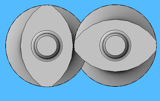


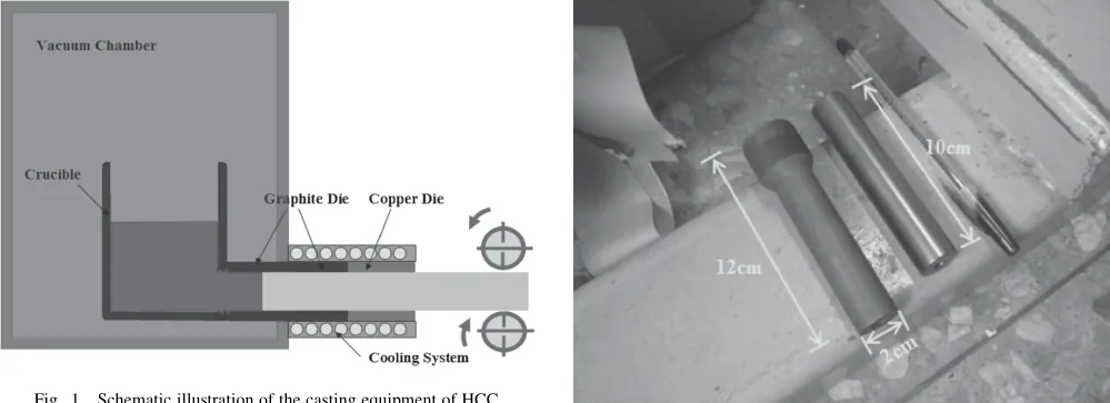


![Figure 1: The moving half of a typical die casting die [2].](https://flow3d.co.kr/wp-content/uploads/image-1792.webp)


![Table 1: Mechanical properties of AA6061 and AA7075 [36].](https://flow3d.co.kr/wp-content/uploads/image-1772.webp)


![Fig 2.2 - Tipology of chamber and its components (adapted from [11, 17]). (a) - Cold chamber; (b) - Hot chamber;](https://flow3d.co.kr/wp-content/uploads/image-1749.webp)


![Figure 2. SEM images of segregated Mo-based coarse particles: (a) clusters of Mo-rich polygonal particles observed in 0.1 Mo, (b) elongated and fragmented Mo-based phases found in 0.3 Mo casting probably deriving from (c) Mo-based needles contained in the Al–Mo10 master alloy; (d–f) corresponding EDS spectra [6].](https://flow3d.co.kr/wp-content/uploads/image-1586.webp)


![Fig. 1. Scanning electron micrographs (a) Mg97Y2Zn1 alloy after solution treatment with grains of the α-Mg matrix (dark grey) and interdendritic LPSO phases (grey) [4], (b) WZ62 after solution treatment [5] and (c) several Mg-Zn-RE alloys after homogenization [3] 1. Scanning electron micrographs (a) Mg97Y2Zn1 alloy after solution treatment with grains of the α-Mg matrix (dark grey) and interdendritic LPSO phases (grey) [4], (b) WZ62 after solution treatment [5] and (c) several Mg-Zn-RE alloys after homogenization [3]](https://flow3d.co.kr/wp-content/uploads/image-1558-scaled.webp)


![Figure 12. American Foundry Association modification levels [15]](https://flow3d.co.kr/wp-content/uploads/image-1538.webp)
![Figure 3. Mechanical and corrosion properties of conventional HPDC magnesium alloys: (a) mechanical properties [25–27] and (b) salt spray test for 1000 hours conducted by Meridian lightweight technologies.](https://flow3d.co.kr/wp-content/uploads/image-1536.webp)


![Obr. 7. Návrh 2 typov zaústení vtokových sústav pre giga odliatky a), b), c) integrálne porovnanie zachyteného vzduchu medzi dvoma konštrukčnými typmi vtokových sústav [1]](https://flow3d.co.kr/wp-content/uploads/image-1529.webp)


![Figure 3. Schematic of the foam degradation process. Source: [43].](https://flow3d.co.kr/wp-content/uploads/image-1440.webp)


![Fig. 1. End uses of zinc [1]](https://flow3d.co.kr/wp-content/uploads/image-1445.webp)


![(c) 24 h; WZ73-1.5 vol% SiC after (d) 1; (e) 12 and (f) 24 h; WZ73-2.5 vol% SiC after (g) 1; (h) 12 and (i) 24 h. Figure 8. XRD patterns of the surface corrosion layers in WZ73 and MMCs after immersing in 1 wt % NaCl solution for (a) 12 h and (b) 24 h. It has been reported that the corrosion reactions of Mg alloys immersed in a neutral aqueous solution proceed by the following reactions [33–35]: Mg → Mg2+ + 2e− (2) 2H2O + 2e− → H2+ + 2OH− (3) Mg2+ +2OH− → Mg(OH)2 (4) Figure 7. Surface morphology of WZ73 after immersing in 1 wt % NaCl solution for (a) 1; (b) 12 and (c) 24 h; WZ73-1.5 vol % SiC after (d) 1; (e) 12 and (f) 24 h; WZ73-2.5 vol % SiC after (g) 1; (h) 12 and (i) 24 h. Metals 2018, 8, x FOR PEER REVIEW 10 of 16 Figure 7. Surface morphology of WZ73 after immersing in 1 wt % NaCl solution for (a) 1; (b) 12 and (c) 24 h; WZ73](https://flow3d.co.kr/wp-content/uploads/image-1425.webp)

![Fig. 1 Progress trend of various metals used for MMCs until 2022[1].](https://flow3d.co.kr/wp-content/uploads/image-1417.webp)


![Figure 5. Images showing backseat applications: (a) 2014 Chevrolet corvette seatback (courtesy of GM); (b) 2015 Mercedes- Benz SLK seatback [37] (courtesy of GF casting solutions) and (c) 2014 BMW i3 seatback [38] (courtesy of BASF).](https://flow3d.co.kr/wp-content/uploads/image-1380.webp)


![Figure 2. Effect of braking electromagnetic fields on the flow fields, (a) No magnetic fields; (b) B = 0.1 T and (c) B = 0.2 T [23].](https://flow3d.co.kr/wp-content/uploads/image-1188.webp)


![Figure 1 Principle of the FDU device [3]](https://flow3d.co.kr/wp-content/uploads/image-1107.webp)
![[그림 7] 마그네슘 휠 물성 비교 1](https://flow3d.co.kr/wp-content/uploads/image-1104.webp)


![Fig. 6: Calculated degassing efficiency as a function of bubble size [40]](https://flow3d.co.kr/wp-content/uploads/image-1080.webp)


![Figure 2.4 Different designs of mechanical stirrers [Harnby et al. 1997].](https://flow3d.co.kr/wp-content/uploads/image-1034.webp)


![Fig. 6. Chemical fluctuations analysis around an APB region on a (111) plane in alloy 0Ti. (a) HAADF-STEM image of the ' precipitate with APBs taken along [011] beam direction. (b) Magnified image of white rectangular marked in (a). (c) Composite chemical map of elements Co, Ni, Al, Mo and W. (d)-(h) Net intensity elemental maps of elements Co, Ni, Al, Mo and W. (i) and (j) EDS line scan integrated along the APB in the region marked in (c).](https://flow3d.co.kr/wp-content/uploads/image-978.webp)


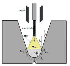
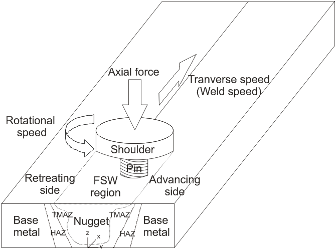
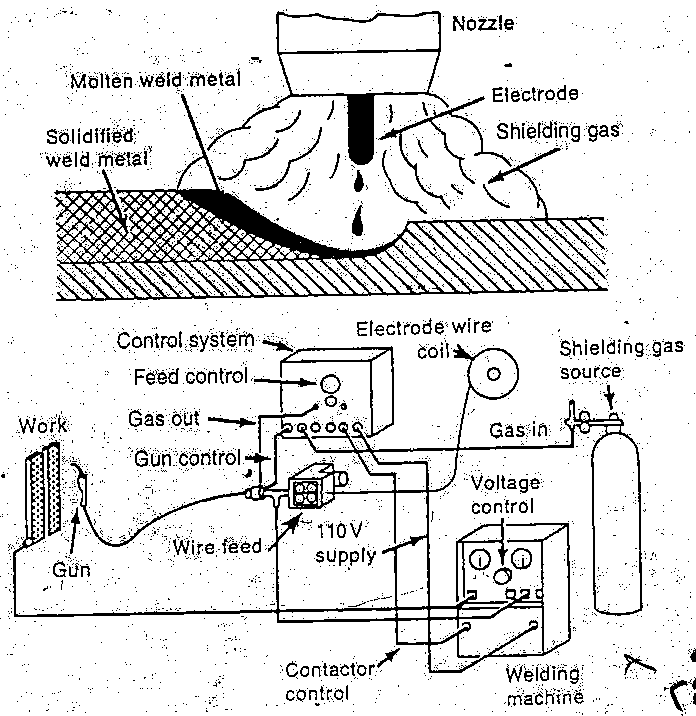
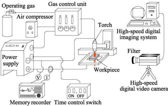


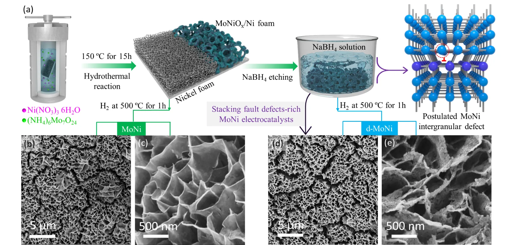


![Obr. 13: Svarovací program s jedním impulsem [2]](https://flow3d.co.kr/wp-content/uploads/image-1702.webp)


![Fig. 1.2: Variation in heat input with the power density of heat source [2]](https://flow3d.co.kr/wp-content/uploads/image-1389.webp)


![Fig. 10. Optical micrograph of an onion ring feature in FSW AA6061/Al2O3/20p crosssection [35].](https://flow3d.co.kr/wp-content/uploads/image-918.webp)


![Fig. 4. Schematic illustration of FCAW process [9].](https://flow3d.co.kr/wp-content/uploads/image-732.webp)


![Figure-1.1 TIG Welding Setup [Ref.: office.pickproducts.com.au]](https://flow3d.co.kr/wp-content/uploads/image-706.webp)


![Figure 1.1 A schematic of Gas Metal Arc Welding Process [4]](https://flow3d.co.kr/wp-content/uploads/image-657.webp)


![Fig. 1. A schematic sketch of a GTAW process [Wikipedia].](https://flow3d.co.kr/wp-content/uploads/image-651.webp)


![Figure 1. a) Sketch of the pier-caisson system considered in this study; b) Top view of a local scour hole, with the contour lines indicating the depth – values are normalized with respect to the maximum depth (after [9]).](https://flow3d.co.kr/wp-content/uploads/image-1629.webp)