1 Institut für Wasserwirtschaft, Hydrologie und Konstruktiven Wasserbau, B.O.K.U. University, Muthgasse 18, 1190 Vienna, (actually Senior Process Engineer at the VTU Engineering in Vienna, Zieglergasse 53/1/24, 1070 Vienna, Austria).2 School of Pedagogical and Technological Education, Department of Civil Engineering Educators, ASPETE Campus, Eirini Station, 15122 Amarousio, Athens, Greece.
Abstract
이 논문은 최초의 아르키메데스 나사 터빈 CFD 모델링 결과에 대한 간략한 견해를 제시하며, 이는 “그리스에서 아르키메데스의 부활: 수리 역학 및 아르키메데스 달팽이관 물레방아의 유체역학적 거동 연구에 대한 기여”라는 제목의 최근 연구에서 수행되었습니다. 그리스 자연 및 기술 수로의 수력 잠재력”. Flow-3D 코드를 기반으로 하는 이 CFD 분석은 일반적인 TAST(Tubular Archimedean Screw Turbines)와 관련이 있으며 몇 TWh 정도의 그리스 자연 및 기술 수로의 중요한 미개발 수력 잠재력을 활용하는 연간 및 수천 MW 범위의 총 설치 용량인 소규모 수력 발전 시스템에 대한 몇 가지 유망한 성능을 보여줍니다.
This paper presents a short view of the first Archimedean Screw Turbines CFD modelling results, which were carried out within the recent research entitled “Rebirth of Archimedes in Greece: contribution to the study of hydraulic mechanics and hydrodynamic behavior of Archimedean cochlear waterwheels, for recovering the hydraulic potential of Greek natural and technical watercourses”. This CFD analysis, based to the Flow-3D code, concerns typical Tubular Archimedean Screw Turbines (TASTs) and shows some promising performances for such small hydropower systems harnessing the important unexploited hydraulic potential of natural and technical watercourses of Greece, of the order of several TWh / year and of a total installed capacity in the range of thousands MWs.
Keywords
CFD; Flow-3D; TAST; Small Hydro; Renewable Energy; Greek Watercourses.
Figure 1. Photorealistic view of an inclined axis TAST (photo A. Stergiopoulou).Figure 3. The spectrum of all the screw axis orientation cases.
Figure 4. Creation of the 3bladed Archimedean Screw with SolidworksFigure 6. “Meshing & Geometry” tab Operations (Flow 3-D).Figure 7. Comparison of Archimedean screw power performances P(W) for Q = 0.15 m3
/s and 0.30m3
/s
and angles of orientation 22ο & 32ο
.Figure 12. Various performances of the Archimedean Screw (MKE/Mean Kinetic Energy, Torque,
Turbulent Kinetic Energy, Turbulent Dissipation) for flow discharge Q = 0.45 m3
/s and an angle of
orientation θ = 32ο
References
[1] A. Stergiopoulou, Computational and experimental investigation of the hydrodynamic behaviour of screw hydro turbine, Ph.D. Thesis, NTUA, 2017. [2] B. Pelikan, A. Lashofer, Verbesserung der Strömungseigenschaften sowie Planungs-und Betriebsoptimierung von Wasserkraftschnecken, Research Project, BOKU University, Vienna, 2012. [3] G. Müller, J. Senior, Simplified theory of Archimedean screws, Journal of Hydraulic Research 47 (5) (2009) 666-669. [4] C. Rorres, The turn of the screw: Optimal design of an Archimedes screw, Journal of Hydraulic Engineering, 80 (2000) 72-80. [5] A. Stergiopoulou, V. Stergiopoulos, Return of Archimedes: Harnessing with new Archimedean spirals the hydraulic potential of the Greek watercourses, in: Proceedings of the Conference for Climate Change, Thessaloniki, 2009. [6] A. Stergiopoulou, V. Stergiopoulos, from the old Archimedean screw pumps to the new Archimedean screw turbines for hydropower production in Greece, in: Proceedings of CEMEPE Conference, Mykonos, June 21-26, 2009.
[7] V. Stergiopoulos, A. Stergiopoulou, E. Kalkani, Quo Vadis Archimedes Nowadays in Greece? Towards Modern Archimedean Turbines for Recovering Greek Small Hydropower Potential, in: Proceedings of 3rd International Scientific “Energy and Climate Change” Conference, Athens, 2010. [8] A. Stergiopoulou, V. Stergiopoulos, E. Κalkani, Greece beyond the horizon of the era of transition: Archimedean screw hydropower development terra incognita, International Journal of Energy and Development, v.6, Issue 6, pp. 627-536, 2015. [9] A. Stergiopoulou, V. Stergiopoulos, E. Κalkani, Experimental and theoretical research of zero head innovative horizontal axis Archimedean screw turbines, Journal of Energy and Development, v.6, Issue 5, pp. 471-478, 2015. [10] A. Stergiopoulou, V. Stergiopoulos, E. Κalkani, Back to the Future: Rediscovering the Archimedean screws as modern turbines for harnessing Greek small hydropower potential, in: Proceedings of the Third International Conference CEMEPE 2011 & SECOTOX, Skiathos, 2011. [11] A. Stergiopoulou, V. Stergiopoulos, Educational Renewable Energy Screw Wheel Technologies for Pico Hydropower Generation, Modern Environmental Science and Engineering, v.4, No.5, pp. 439- 445, May 2018. [12] A. Stergiopoulou, V. Stergiopoulos, Educational Renewable Energy Screw Wheel Technologies for Pico Hydropower Generation, Modern Environmental Science and Engineering, v.4, No.5, pp. 439- 445, May 2018. [13] A. Stergiopoulou, V. Stergiopoulos, Towards an inventory of the archimedean small hydropower potential of Greece, INTERNATIONAL JOURNAL OF ENERGY AND ENVIRONMENT Volume 11, Issue 2, 2020 pp.137-144. [14] Flow Science, FLOW-3D Manual, 2013. [15] K. Versteeg and W. Malalasekera, An Introduction to Computational Fluid Dynamics, Pearson, 2007. [16] C. Hirsch, Numerical Computation of internal and external flows: The fundamentals of Computational Fluid dynamics, John Wiley & Sons, 2007. [17] A. Stergiopoulou, V. Stergiopoulos and E. Kalkani, An eagle’s CFD view of Studying Innovative Archimedean Screw Renewable Hydraulic Energy Systems, Proceedings of the 4th International Conference on Environmental Management, Engineering, Planning and Economics (CEMEPE) and SECOTOX Conference, Mykonos island, Greece, pp.454-460 June 24-28, 2013. [18] A. Stergiopoulou, V. Stergiopoulos, A., E. Kalkani, Computational Fluid Dynamics Study on a 3D Graphic Solid Model of Archimedean Screw Turbines, Fresenius Environmental Bulletin, vol.23- No1, 2014. [19] Α. Stergiopoulou, Kalkani E., “Towards a First C.F.D. Study of Innovative Archimedean Inclined Axis Hydropower Turbines”, International Journal of Engineering Research & Technology (IJERT), Vol. 2 Issue 9, September – 2013, pp. 193-199. [20] A. Stergiopoulou, V. Stergiopoulos, A first CFD study of small hydro energy recovery from the Attica water supply network, INTERNATIONAL JOURNAL OF ENERGY AND ENVIRONMENT, Volume 11, Issue 3, 2020 pp.157-166.
결합된 Bi-level 메타휴리스틱 접근법을 사용한 해양 재생 에너지 변환기의 설계 최적화
Erfan Amini a1, Mahdieh Nasiri b1, Navid Salami Pargoo a, Zahra Mozhgani c, Danial Golbaz d, Mehrdad Baniesmaeil e, Meysam Majidi Nezhad f, Mehdi Neshat gj, Davide Astiaso Garcia h, Georgios Sylaios i
Abstract
In recent years, there has been an increasing interest in renewable energies in view of the fact that fossil fuels are the leading cause of catastrophic environmental consequences. Ocean wave energy is a renewable energy source that is particularly prevalent in coastal areas. Since many countries have tremendous potential to extract this type of energy, a number of researchers have sought to determine certain effective factors on wave converters’ performance, with a primary emphasis on ambient factors. In this study, we used metaheuristic optimization methods to investigate the effects of geometric factors on the performance of an Oscillating Surge Wave Energy Converter (OSWEC), in addition to the effects of hydrodynamic parameters. To do so, we used CATIA software to model different geometries which were then inserted into a numerical model developed in Flow3D software. A Ribed-surface design of the converter’s flap is also introduced in this study to maximize wave-converter interaction. Besides, a Bi-level Hill Climbing Multi-Verse Optimization (HCMVO) method was also developed for this application. The results showed that the converter performs better with greater wave heights, flap freeboard heights, and shorter wave periods. Additionally, the added ribs led to more wave-converter interaction and better performance, while the distance between the flap and flume bed negatively impacted the performance. Finally, tracking the changes in the five-dimensional objective function revealed the optimum value for each parameter in all scenarios. This is achieved by the newly developed optimization algorithm, which is much faster than other existing cutting-edge metaheuristic approaches.
Keywords
Wave Energy Converter
OSWEC
Hydrodynamic Effects
Geometric Design
Metaheuristic Optimization
Multi-Verse Optimizer
1. Introduction
The increase in energy demand, the limitations of fossil fuels, as well as environmental crises, such as air pollution and global warming, are the leading causes of calling more attention to harvesting renewable energy recently [1], [2], [3]. While still in its infancy, ocean wave energy has neither reached commercial maturity nor technological convergence. In recent decades, remarkable progress has been made in the marine energy domain, which is still in the early stage of development, to improve the technology performance level (TPL) [4], [5]and technology readiness level (TRL) of wave energy converters (WECs). This has been achieved using novel modeling techniques [6], [7], [8], [9], [10], [11], [12], [13], [14] to gain the following advantages [15]: (i) As a source of sustainable energy, it contributes to the mix of energy resources that leads to greater diversity and attractiveness for coastal cities and suppliers. [16] (ii) Since wave energy can be exploited offshore and does not require any land, in-land site selection would be less expensive and undesirable visual effects would be reduced. [17] (iii) When the best layout and location of offshore site are taken into account, permanent generation of energy will be feasible (as opposed to using solar energy, for example, which is time-dependent) [18].
In general, the energy conversion process can be divided into three stages in a WEC device, including primary, secondary, and tertiary stages [19], [20]. In the first stage of energy conversion, which is the subject of this study, the wave power is converted to mechanical power by wave-structure interaction (WSI) between ocean waves and structures. Moreover, the mechanical power is transferred into electricity in the second stage, in which mechanical structures are coupled with power take-off systems (PTO). At this stage, optimal control strategies are useful to tune the system dynamics to maximize power output [10], [13], [12]. Furthermore, the tertiary energy conversion stage revolves around transferring the non-standard AC power into direct current (DC) power for energy storage or standard AC power for grid integration [21], [22]. We discuss only the first stage regardless of the secondary and tertiary stages. While Page 1 of 16 WECs include several categories and technologies such as terminators, point absorbers, and attenuators [15], [23], we focus on oscillating surge wave energy converters (OSWECs) in this paper due to its high capacity for industrialization [24].
Over the past two decades, a number of studies have been conducted to understand how OSWECs’ structures and interactions between ocean waves and flaps affect converters performance. Henry et al.’s experiment on oscillating surge wave energy converters is considered as one of the most influential pieces of research [25], which demonstrated how the performance of oscillating surge wave energy converters (OSWECs) is affected by seven different factors, including wave period, wave power, flap’s relative density, water depth, free-board of the flap, the gap between the tubes, gap underneath the flap, and flap width. These parameters were assessed in their two models in order to estimate the absorbed energy from incoming waves [26], [27]. In addition, Folly et al. investigated the impact of water depth on the OSWECs performance analytically, numerically, and experimentally. According to this and further similar studies, the average annual incident wave power is significantly reduced by water depth. Based on the experimental results, both the surge wave force and the power capture of OSWECs increase in shallow water [28], [29]. Following this, Sarkar et al. found that under such circumstances, the device that is located near the coast performs much better than those in the open ocean [30]. On the other hand, other studies are showing that the size of the converter, including height and width, is relatively independent of the location (within similar depth) [31]. Subsequently, Schmitt et al. studied OSWECs numerically and experimentally. In fact, for the simulation of OSWEC, OpenFOAM was used to test the applicability of Reynolds-averaged Navier-Stokes (RANS) solvers. Then, the experimental model reproduced the numerical results with satisfying accuracy [32]. In another influential study, Wang et al. numerically assessed the effect of OSWEC’s width on their performance. According to their findings, as converter width increases, its efficiency decreases in short wave periods while increases in long wave periods [33]. One of the main challenges in the analysis of the OSWEC is the coupled effect of hydrodynamic and geometric variables. As a result, numerous cutting-edge geometry studies have been performed in recent years in order to find the optimal structure that maximizes power output and minimizes costs. Garcia et al. reviewed hull geometry optimization studies in the literature in [19]. In addition, Guo and Ringwood surveyed geometric optimization methods to improve the hydrodynamic performance of OSWECs at the primary stage [14]. Besides, they classified the hull geometry of OSWECs based on Figure 1. Subsequently, Whittaker et al. proposed a different design of OSWEC called Oyster2. There have been three examples of different geometries of oysters with different water depths. Based on its water depth, they determined the width and height of the converter. They also found that in the constant wave period the less the converter’s width, the less power captures the converter has [34]. Afterward, O’Boyle et al. investigated a type of OSWEC called Oyster 800. They compared the experimental and numerical models with the prototype model. In order to precisely reproduce the shape, mass distribution, and buoyancy properties of the prototype, a 40th-scale experimental model has been designed. Overall, all the models were fairly accurate according to the results [35].
Inclusive analysis of recent research avenues in the area of flap geometry has revealed that the interaction-based designs of such converters are emerging as a novel approach. An initiative workflow is designed in the current study to maximizing the wave energy extrication by such systems. To begin with, a sensitivity analysis plays its role of determining the best hydrodynamic values for installing the converter’s flap. Then, all flap dimensions and characteristics come into play to finalize the primary model. Following, interactive designs is proposed to increase the influence of incident waves on the body by adding ribs on both sides of the flap as a novel design. Finally, a new bi-level metaheuristic method is proposed to consider the effects of simultaneous changes in ribs properties and other design parameters. We hope this novel approach will be utilized to make big-scale projects less costly and justifiable. The efficiency of the method is also compared with four well known metaheuristic algorithms and out weight them for this application.
This paper is organized as follows. First, the research methodology is introduced by providing details about the numerical model implementation. To that end, we first introduced the primary model’s geometry and software details. That primary model is later verified with a benchmark study with regard to the flap angle of rotation and water surface elevation. Then, governing equations and performance criteria are presented. In the third part of the paper, we discuss the model’s sensitivity to lower and upper parts width (we proposed a two cross-sectional design for the flap), bottom elevation, and freeboard. Finally, the novel optimization approach is introduced in the final part and compared with four recent metaheuristic algorithms.
2. Numerical Methods
In this section, after a brief introduction of the numerical software, Flow3D, boundary conditions are defined. Afterwards, the numerical model implementation, along with primary model properties are described. Finally, governing equations, as part of numerical process, are discussed.
2.1. Model Setup
FLOW-3D is a powerful and comprehensive CFD simulation platform for studying fluid dynamics. This software has several modules to solve many complex engineering problems. In addition, modeling complex flows is simple and effective using FLOW-3D’s robust meshing capabilities [36]. Interaction between fluid and moving objects might alter the computational range. Dynamic meshes are used in our modeling to take these changes into account. At each time step, the computational node positions change in order to adapt the meshing area to the moving object. In addition, to choose mesh dimensions, some factors are taken into account such as computational accuracy, computational time, and stability. The final grid size is selected based on the detailed procedure provided in [37]. To that end, we performed grid-independence testing on a CFD model using three different mesh grid sizes of 0.01, 0.015, and 0.02 meters. The problem geometry and boundary conditions were defined the same, and simulations were run on all three grids under the same conditions. The predicted values of the relevant variable, such as velocity, was compared between the grids. The convergence behavior of the numerical solution was analyzed by calculating the relative L2 norm error between two consecutive grids. Based on the results obtained, it was found that the grid size of 0.02 meters showed the least error, indicating that it provided the most accurate and reliable solution among the three grids. Therefore, the grid size of 0.02 meters was selected as the optimal spatial resolution for the mesh grid.
In this work, the flume dimensions are 10 meters long, 0.1 meters wide, and 2.2 meters high, which are shown in figure2. In addition, input waves with linear characteristics have a height of 0.1 meters and a period of 1.4 seconds. Among the linear wave methods included in this software, RNGk-ε and k- ε are appropriate for turbulence model. The research of Lopez et al. shows that RNGk- ε provides the most accurate simulation of turbulence in OSWECs [21]. We use CATIA software to create the flap primary model and other innovative designs for this project. The flap measures 0.1 m x 0.65 m x 0.360 m in x, y and z directions, respectively. In Figure 3, the primary model of flap and its dimensions are shown. In this simulation, five boundaries have been defined, including 1. Inlet, 2. Outlet, 3. Converter flap, 4. Bed flume, and 5. Water surface, which are shown in figure 2. Besides, to avoid wave reflection in inlet and outlet zones, Flow3D is capable of defining some areas as damping zones, the length of which has to be one to one and a half times the wavelength. Therefore, in the model, this length is considered equal to 2 meters. Furthermore, there is no slip in all the boundaries. In other words, at every single time step, the fluid velocity is zero on the bed flume, while it is equal to the flap velocity on the converter flap. According to the wave theory defined in the software, at the inlet boundary, the water velocity is called from the wave speed to be fed into the model.
2.2. Verification
In the current study, we utilize the Schmitt experimental model as a benchmark for verification, which was developed at the Queen’s University of Belfast. The experiments were conducted on the flap of the converter, its rotation, and its interaction with the water surface. Thus, the details of the experiments are presented below based up on the experimental setup’s description [38]. In the experiment, the laboratory flume has a length of 20m and a width of 4.58m. Besides, in order to avoid incident wave reflection, a wave absorption source is devised at the end of the left flume. The flume bed, also, includes two parts with different slops. The flap position and dimensions of the flume can be seen in Figure4. In addition, a wave-maker with 6 paddles is installed at one end. At the opposite end, there is a beach with wire meshes. Additionally, there are 6 indicators to extract the water level elevation. In the flap model, there are three components: the fixed support structure, the hinge, and the flap. The flap measures 0.1m x 0.65m x 0.341m in x, y and z directions, respectively. In Figure5, the details are given [32]. The support structure consists of a 15 mm thick stainless steel base plate measuring 1m by 1.4m, which is screwed onto the bottom of the tank. The hinge is supported by three bearing blocks. There is a foam centerpiece on the front and back of the flap which is sandwiched between two PVC plates. Enabling changes of the flap, three metal fittings link the flap to the hinge. Moreover, in this experiment, the selected wave is generated based on sea wave data at scale 1:40. The wave height and the wave period are equal to 0.038 (m) and 2.0625 (s), respectively, which are tantamount to a wave with a period of 13 (s) and a height of 1.5 (m).
Two distinct graphs illustrate the numerical and experi-mental study results. Figure6 and Figure7 are denoting the angle of rotation of flap and surface elevation in computational and experimental models, respectively. The two figures roughly represent that the numerical and experimental models are a good match. However, for the purpose of verifying the match, we calculated the correlation coefficient (C) and root mean square error (RMSE). According to Figure6, correlation coefficient and RMSE are 0.998 and 0.003, respectively, and in Figure7 correlation coefficient and RMSE are respectively 0.999 and 0.001. Accordingly, there is a good match between the numerical and empirical models. It is worth mentioning that the small differences between the numerical and experimental outputs may be due to the error of the measuring devices and the calibration of the data collection devices.
Including continuity equation and momentum conserva- tion for incompressible fluid are given as [32], [39]:(1)
where P represents the pressure, g denotes gravitational acceleration, u represents fluid velocity, and Di is damping coefficient. Likewise, the model uses the same equation. to calculate the fluid velocity in other directions as well. Considering the turbulence, we use the two-equation model of RNGK- ε. These equations are:
(3)��t(��)+����(����)=����[�eff�������]+��-��and(4)���(��)+����(����)=����[�eff�������]+�1�∗����-��2��2�Where �2� and �1� are constants. In addition, �� and �� represent the turbulent Prandtl number of � and k, respectively.
�� also denote the production of turbulent kinetic energy of k under the effect of velocity gradient, which is calculated as follows:(5)��=�eff[�����+�����]�����(6)�eff=�+��(7)�eff=�+��where � is molecular viscosity,�� represents turbulence viscosity, k denotes kinetic energy, and ∊∊ is energy dissipation rate. The values of constant coefficients in the two-equation RNGK ∊-∊ model is as shown in the Table 1[40].Table 2.
Table 1. Constant coefficients in RNGK-∊ model
Factors
�
�0
�1
�2
��
��
��
Quantity
0.012
4.38
1.42
1.68
1.39
1.39
0.084
Table 2. Flap properties
Joint height (m)
0.476
Height of the center of mass (m)
0.53
Weight (Kg)
10.77
It is worth mentioning that the volume of fluid method is used to separate water and air phases in this software [41]. Below is the equation of this method [40].(8)����+����(���)=0where α and 1 − α are portion of water phase and air phase, respectively. As a weighting factor, each fluid phase portion is used to determine the mixture properties. Finally, using the following equations, we calculate the efficiency of converters [42], [34], [43]:(9)�=14|�|2�+�2+(�+�a)2(�n2-�2)2where �� represents natural frequency, I denotes the inertia of OSWEC, Ia is the added inertia, F is the complex wave force, and B denotes the hydrodynamic damping coefficient. Afterward, the capture factor of the converter is calculated by [44]:(10)��=�1/2��2����gw where �� represents the capture factor, which is the total efficiency of device per unit length of the wave crest at each time step [15], �� represent the dimensional amplitude of the incident wave, w is the flap’s width, and Cg is the group velocity of the incident wave, as below:(11)��=��0·121+2�0ℎsinh2�0ℎwhere �0 denotes the wave number, h is water depth, and H is the height of incident waves.
According to previous sections ∊,����-∊ modeling is used for all models simulated in this section. For this purpose, the empty boundary condition is used for flume walls. In order to preventing wave reflection at the inlet and outlet of the flume, the length of wave absorption is set to be at least one incident wavelength. In addition, the structured mesh is chosen, and the mesh dimensions are selected in two distinct directions. In each model, all grids have a length of 2 (cm) and a height of 1 (cm). Afterwards, as an input of the software for all of the models, we define the time step as 0.001 (s). Moreover, the run time of every simulation is 30 (s). As mentioned before, our primary model is Schmitt model, and the flap properties is given in table2. For all simulations, the flume measures 15 meters in length and 0.65 meters in width, and water depth is equal to 0.335 (m). The flap is also located 7 meters from the flume’s inlet.
Finally, in order to compare the results, the capture factor is calculated for each simulation and compared to the primary model. It is worth mentioning that capture factor refers to the ratio of absorbed wave energy to the input wave energy.
According to primary model simulation and due to the decreasing horizontal velocity with depth, the wave crest has the highest velocity. Considering the fact that the wave’s orbital velocity causes the flap to move, the contact between the upper edge of the flap and the incident wave can enhance its performance. Additionally, the numerical model shows that the dynamic pressure decreases as depth increases, and the hydrostatic pressure increases as depth increases.
To determine the OSWEC design, it is imperative to understand the correlation between the capture factor, wave period, and wave height. Therefore, as it is shown in Figure8, we plot the change in capture factor over the variations in wave period and wave height in 3D and 2D. In this diagram, the first axis features changes in wave period, the second axis displays changes in wave height, and the third axis depicts changes in capture factor. According to our wave properties in the numerical model, the wave period and wave height range from 2 to 14 seconds and 2 to 8 meters, respectively. This is due to the fact that the flap does not oscillate if the wave height is less than 2 (m), and it does not reverse if the wave height is more than 8 (m). In addition, with wave periods more than 14 (s), the wavelength would be so long that it would violate the deep-water conditions, and with wave periods less than 2 (s), the flap would not oscillate properly due to the shortness of wavelength. The results of simulation are shown in Figure 8. As it can be perceived from Figure 8, in a constant wave period, the capture factor is in direct proportion to the wave height. It is because of the fact that waves with more height have more energy to rotate the flap. Besides, in a constant wave height, the capture factor increases when the wave period increases, until a given wave period value. However, the capture factor falls after this point. These results are expected since the flap’s angular displacement is not high in lower wave periods, while the oscillating motion of that is not fast enough to activate the power take-off system in very high wave periods.
As is shown in Figure 9, we plot the change in capture factor over the variations in wave period (s) and water depth (m) in 3D. As it can be seen in this diagram, the first axis features changes in water depth (m), the second axis depicts the wave period (s), and the third axis displays OSWEC’s capture factor. The wave period ranges from 0 to 10 seconds based on our wave properties, which have been adopted from Schmitt’s model, while water depth ranges from 0 to 0.5 meters according to the flume and flap dimensions and laboratory limitations. According to Figure9, for any specific water depth, the capture factor increases in a varying rate when the wave period increases, until a given wave period value. However, the capture factor falls steadily after this point. In fact, the maximum capture factor occurs when the wave period is around 6 seconds. This trend is expected since, in a specific water depth, the flap cannot oscillate properly when the wavelength is too short. As the wave period increases, the flap can oscillate more easily, and consequently its capture factor increases. However, the capture factor drops in higher wave periods because the wavelength is too large to move the flap. Furthermore, in a constant wave period, by changing the water depth, the capture factor does not alter. In other words, the capture factor does not depend on the water depth when it is around its maximum value.
3. Sensitivity Analysis
Based on previous studies, in addition to the flap design, the location of the flap relative to the water surface (freeboard) and its elevation relative to the flume bed (flap bottom elevation) play a significant role in extracting energy from the wave energy converter. This study measures the sensitivity of the model to various parameters related to the flap design including upper part width of the flap, lower part width of the flap, the freeboard, and the flap bottom elevation. Moreover, as a novel idea, we propose that the flap widths differ in the lower and upper parts. In Figure10, as an example, a flap with an upper thickness of 100 (mm) and a lower thickness of 50 (mm) and a flap with an upper thickness of 50 (mm) and a lower thickness of 100 (mm) are shown. The influence of such discrepancy between the widths of the upper and lower parts on the interaction between the wave and the flap, or in other words on the capture factor, is evaluated. To do so, other parameters are remained constant, such as the freeboard, the distance between the flap and the flume bed, and the wave properties.
In Figure11, models are simulated with distinct upper and lower widths. As it is clear in this figure, the first axis depicts the lower part width of the flap, the second axis indicates the upper part width of the flap, and the colors represent the capture factor values. Additionally, in order to consider a sufficient range of change, the flap thickness varies from half to double the value of the primary model for each part.
According to this study, the greater the discrepancy in these two parts, the lower the capture factor. It is on account of the fact that when the lower part of the flap is thicker than the upper part, and this thickness difference in these two parts is extremely conspicuous, the inertia against the motion is significant at zero degrees of rotation. Consequently, it is difficult to move the flap, which results in a low capture factor. Similarly, when the upper part of the flap is thicker than the lower part, and this thickness difference in these two parts is exceedingly noticeable, the inertia is so great that the flap can not reverse at the maximum degree of rotation. As the results indicate, the discrepancy can enhance the performance of the converter if the difference between these two parts is around 20%. As it is depicted in the Figure11, the capture factor reaches its own maximum amount, when the lower part thickness is from 5 to 6 (cm), and the upper part thickness is between 6 and 7 (cm). Consequently, as a result of this discrepancy, less material will be used, and therefore there will be less cost.
As illustrated in Figure12, this study examines the effects of freeboard (level difference between the flap top and water surface) and the flap bottom elevation (the distance between the flume bed and flap bottom) on the converter performance. In this diagram, the first axis demonstrates the freeboard and the second axis on the left side displays the flap bottom elevation, while the colors indicate the capture factor. In addition, the feasible range of freeboard is between -15 to 15 (cm) due to the limitation of the numerical model, so that we can take the wave slamming and the overtopping into consideration. Additionally, based on the Schmitt model and its scaled model of 1:40 of the base height, the flap bottom should be at least 9 (cm) high. Since the effect of surface waves is distributed over the depth of the flume, it is imperative to maintain a reasonable flap height exposed to incoming waves. Thus, the maximum flap bottom elevation is limited to 19 (cm). As the Figure12 pictures, at constant negative values of the freeboard, the capture factor is in inverse proportion with the flap bottom elevation, although slightly.
Furthermore, at constant positive values of the freeboard, the capture factor fluctuates as the flap bottom elevation decreases while it maintains an overall increasing trend. This is on account of the fact that increasing the flap bottom elevation creates turbulence flow behind the flap, which encumbers its rotation, as well as the fact that the flap surface has less interaction with the incoming waves. Furthermore, while keeping the flap bottom elevation constant, the capture factor increases by raising the freeboard. This is due to the fact that there is overtopping with adverse impacts on the converter performance when the freeboard is negative and the flap is under the water surface. Besides, increasing the freeboard makes the wave slam more vigorously, which improves the converter performance.
Adding ribs to the flap surface, as shown in Figure13, is a novel idea that is investigated in the next section. To achieve an optimized design for the proposed geometry of the flap, we determine the optimal number and dimensions of ribs based on the flap properties as our decision variables in the optimization process. As an example, Figure13 illustrates a flap with 3 ribs on each side with specific dimensions.
Figure14 shows the flow velocity field around the flap jointed to the flume bed. During the oscillation of the flap, the pressure on the upper and lower surfaces of the flap changes dynamically due to the changing angle of attack and the resulting change in the direction of fluid flow. As the flap moves upwards, the pressure on the upper surface decreases, and the pressure on the lower surface increases. Conversely, as the flap moves downwards, the pressure on the upper surface increases, and the pressure on the lower surface decreases. This results in a cyclic pressure variation around the flap. Under certain conditions, the pressure field around the flap can exhibit significant variations in magnitude and direction, forming vortices and other flow structures. These flow structures can affect the performance of the OSWEC by altering the lift and drag forces acting on the flap.
4. Design Optimization
We consider optimizing the design parameters of the flap of converter using a nature-based swarm optimization method, that fall in the category of metaheuristic algorithms [45]. Accordingly, we choose four state-of-the-art algorithms to perform an optimization study. Then, based on their performances to achieve the highest capture factor, one of them will be chosen to be combined with the Hill Climb algorithm to carry out a local search. Therefore, in the remainder of this section, we discuss the search process of each algorithm and visualize their performance and convergence curve as they try to find the best values for decision variables.
4.1. Metaheuristic Approaches
As the first considered algorithm, the Gray Wolf Optimizer (GWO) algorithm simulates the natural leadership and hunting performance of gray wolves which tend to live in colonies. Hunters must obey the alpha wolf, the leader, who is responsible for hunting. Then, the beta wolf is at the second level of the gray wolf hierarchy. A subordinate of alpha wolf, beta stands under the command of the alpha. At the next level in this hierarchy, there are the delta wolves. They are subordinate to the alpha and beta wolves. This category of wolves includes scouts, sentinels, elders, hunters, and caretakers. In this ranking, omega wolves are at the bottom, having the lowest level and obeying all other wolves. They are also allowed to eat the prey just after others have eaten. Despite the fact that they seem less important than others, they are really central to the pack survival. Since, it has been shown that without omega wolves, the entire pack would experience some problems like fighting, violence, and frustration. In this simulation, there are three primary steps of hunting including searching, surrounding, and finally attacking the prey. Mathematically model of gray wolves’ hunting technique and their social hierarchy are applied in determined by optimization. this study. As mentioned before, gray wolves can locate their prey and surround them. The alpha wolf also leads the hunt. Assuming that the alpha, beta, and delta have more knowledge about prey locations, we can mathematically simulate gray wolf hunting behavior. Hence, in addition to saving the top three best solutions obtained so far, we compel the rest of the search agents (also the omegas) to adjust their positions based on the best search agent. Encircling behavior can be mathematically modeled by the following equations: [46].(12)�→=|�→·��→(�)-�→(�)|(13)�→(�+1)=��→(�)-�→·�→(14)�→=2.�2→(15)�→=2�→·�1→-�→Where �→indicates the position vector of gray wolf, ��→ defines the vector of prey, t indicates the current iteration, and �→and �→are coefficient vectors. To force the search agent to diverge from the prey, we use �→ with random values greater than 1 or less than -1. In addition, C→ contains random values in the range [0,2], and �→ 1 and �2→ are random vectors in [0,1]. The second considered technique is the Moth Flame Optimizer (MFO) algorithm. This method revolves around the moths’ navigation mechanism, which is realized by positioning themselves and maintaining a fixed angle relative to the moon while flying. This effective mechanism helps moths to fly in a straight path. However, when the source of light is artificial, maintaining an angle with the light leads to a spiral flying path towards the source that causes the moth’s death [47]. In MFO algorithm, moths and flames are both solutions. The moths are actual search agents that fly in hyper-dimensional space by changing their position vectors, and the flames are considered pins that moths drop when searching the search space [48]. The problem’s variables are the position of moths in the space. Each moth searches around a flame and updates it in case of finding a better solution. The fitness value is the return value of each moth’s fitness (objective) function. The position vector of each moth is passed to the fitness function, and the output of the fitness function is assigned to the corresponding moth. With this mechanism, a moth never loses its best solution [49]. Some attributes of this algorithm are as follows:
•It takes different values to converge moth in any point around the flame.
•Distance to the flame is lowered to be eventually minimized.
•When the position gets closer to the flame, the updated positions around the flame become more frequent.
As another method, the Multi-Verse Optimizer is based on a multiverse theory which proposes there are other universes besides the one in which we all live. According to this theory, there are more than one big bang in the universe, and each big bang leads to the birth of a new universe [50]. Multi-Verse Optimizer (MVO) is mainly inspired by three phenomena in cosmology: white holes, black holes, and wormholes. A white hole has never been observed in our universe, but physicists believe the big bang could be considered a white hole [51]. Black holes, which behave completely in contrast to white holes, attract everything including light beams with their extremely high gravitational force [52]. In the multiverse theory, wormholes are time and space tunnels that allow objects to move instantly between any two corners of a universe (or even simultaneously from one universe to another) [53]. Based on these three concepts, mathematical models are designed to perform exploration, exploitation, and local search, respectively. The concept of white and black holes is implied as an exploration phase, while the concept of wormholes is considered as an exploitation phase by MVO. Additionally, each solution is analogous to a universe, and each variable in the solution represents an object in that universe. Furthermore, each solution is assigned an inflation rate, and the time is used instead of iterations. Following are the universe rules in MVO:
•The possibility of having white hole increases with the inflation rate.
•The possibility of having black hole decreases with the inflation rate.
•Objects tend to pass through black holes more frequently in universes with lower inflation rates.
•Regardless of inflation rate, wormholes may cause objects in universes to move randomly towards the best universe. [54]
Modeling the white/black hole tunnels and exchanging objects of universes mathematically was accomplished by using the roulette wheel mechanism. With every iteration, the universes are sorted according to their inflation rates, then, based on the roulette wheel, the one with the white hole is selected as the local extremum solution. This is accomplished through the following steps:
Assume that
(16)���=����1<��(��)����1≥��(��)
Where ��� represents the jth parameter of the ith universe, Ui indicates the ith universe, NI(Ui) is normalized inflation rate of the ith universe, r1 is a random number in [0,1], and j xk shows the jth parameter of the kth universe selected by a roulette wheel selection mechanism [54]. It is assumed that wormhole tunnels always exist between a universe and the best universe formed so far. This mechanism is as follows:(17)���=if�2<���:��+���×((���-���)×�4+���)�3<0.5��-���×((���-���)×�4+���)�3≥0.5����:���where Xj indicates the jth parameter of the best universe formed so far, TDR and WEP are coefficients, where Xj indicates the jth parameter of the best universelbjshows the lower bound of the jth variable, ubj is the upper bound of the jth variable, and r2, r3, and r4 are random numbers in [1], [54].
Finally, one of the newest optimization algorithms is WOA. The WOA algorithm simulates the movement of prey and the whale’s discipline when looking for their prey. Among several species, Humpback whales have a specific method of hunting [55]. Humpback whales can recognize the location of prey and encircle it before hunting. The optimal design position in the search space is not known a priori, and the WOA algorithm assumes that the best candidate solution is either the target prey or close to the optimum. This foraging behavior is called the bubble-net feeding method. Two maneuvers are associated with bubbles: upward spirals and double loops. A unique behavior exhibited only by humpback whales is bubble-net feeding. In fact, The WOA algorithm starts with a set of random solutions. At each iteration, search agents update their positions for either a randomly chosen search agent or the best solution obtained so far [56], [55]. When the best search agent is determined, the other search agents will attempt to update their positions toward that agent. It is important to note that humpback whales swim around their prey simultaneously in a circular, shrinking circle and along a spiral-shaped path. By using a mathematical model, the spiral bubble-net feeding maneuver is optimized. The following equation represents this behavior:(18)�→(�+1)=�′→·�bl·cos(2��)+�∗→(�)
Where:(19)�′→=|�∗→(�)-�→(�)|
X→(t+ 1) indicates the distance of the it h whale to the prey (best solution obtained so far),� is a constant for defining the shape of the logarithmic spiral, l is a random number in [−1,1], and dot (.) is an element-by-element multiplication [55].
Comparing the four above-mentioned methods, simulations are run with 10 search agents for 400 iterations. In Figure 15, there are 20 plots the optimal values of different parameters in optimization algorithms. The five parameters of this study are freeboard, bottom elevations, number of ribs on the converter, rib thickness, and rib Height. The optimal value for each was found by optimization algorithms, naming WOA, MVO, MFO, and GWO. By looking through the first row, the freeboard parameter converges to its maximum possible value in the optimization process of GWO after 300 iterations. Similarly, MFO finds the same result as GWO. In contrast, the freeboard converges to its minimum possible value in MVO optimizing process, which indicates positioning the converter under the water. Furthermore, WOA found the optimal value of freeboard as around 0.02 after almost 200 iterations. In the second row, the bottom elevation is found at almost 0.11 (m) in all algorithms; however, the curves follow different trends in each algorithm. The third row shows the number of ribs, where results immediately reveal that it should be over 4. All algorithms coincide at 5 ribs as the optimal number in this process. The fourth row displays the trends of algorithms to find optimal rib thickness. MFO finds the optimal value early and sets it to around 0.022, while others find the same value in higher iterations. Finally, regarding the rib height, MVO, MFO, and GWO state that the optimal value is 0.06 meters, but WOA did not find a higher value than 0.039.
4.2. HCMVO Bi-level Approach
Despite several strong search characteristics of MVO and its high performance in various optimization problems, it suffers from a few deficiencies in local and global search mechanisms. For instance, it is trapped in the local optimum when wormholes stochastically generate many solutions near the best universe achieved throughout iterations, especially in solving complex multimodal problems with high dimensions [57]. Furthermore, MVO needs to be modified by an escaping strategy from the local optima to enhance the global search abilities. To address these shortages, we propose a fast and effective meta-algorithm (HCMVO) to combine MVO with a Random-restart hill-climbing local search. This meta-algorithm uses MVO on the upper level to develop global tracking and provide a range of feasible and proper solutions. The hill-climbing algorithm is designed to develop a comprehensive neighborhood search around the best-found solution proposed by the upper-level (MVO) when MVO is faced with a stagnation issue or falling into a local optimum. The performance threshold is formulated as follows.(20)Δ����THD=∑�=1�����TH��-����TH��-1�where BestTHDis the best-found solution per generation, andM is related to the domain of iterations to compute the average performance of MVO. If the proposed best solution by the local search is better than the initial one, the global best of MVO will be updated. HCMVO iteratively runs hill climbing when the performance of MVO goes down, each time with an initial condition to prepare for escaping such undesirable situations. In order to get a better balance between exploration and exploitation, the search step size linearly decreases as follows:(21)��=��-����Ma�iter��+1where iter and Maxiter are the current iteration and maximum number of evaluation, respectively. �� stands for the step size of the neighborhood search. Meanwhile, this strategy can improve the convergence rate of MVO compared with other algorithms.
Algorithm 1 shows the technical details of the proposed optimization method (HCMVO). The initial solution includes freeboard (�), bottom elevation (�), number of ribs (Nr), rib thickness (�), and rib height(�).
5. Conclusion
The high trend of diminishing worldwide energy resources has entailed a great crisis upon vulnerable societies. To withstand this effect, developing renewable energy technologies can open doors to a more reliable means, among which the wave energy converters will help the coastal residents and infrastructure. This paper set out to determine the optimized design for such devices that leads to the highest possible power output. The main goal of this research was to demonstrate the best design for an oscillating surge wave energy converter using a novel metaheuristic optimization algorithm. In this regard, the methodology was devised such that it argued the effects of influential parameters, including wave characteristics, WEC design, and interaction criteria.
To begin with, a numerical model was developed in Flow 3D software to simulate the response of the flap of a wave energy converter to incoming waves, followed by a validation study based upon a well-reputed experimental study to verify the accuracy of the model. Secondly, the hydrodynamics of the flap was investigated by incorporating the turbulence. The effect of depth, wave height, and wave period are also investigated in this part. The influence of two novel ideas on increasing the wave-converter interaction was then assessed: i) designing a flap with different widths in the upper and lower part, and ii) adding ribs on the surface of the flap. Finally, four trending single-objective metaheuristic optimization methods
Empty Cell
Algorithm 1:Hill Climb Multiverse Optimization
01:
procedure HCMVO
02:
�=30,�=5▹���������������������������������
03:
�=〈F1,B1,N,R,H1〉,…〈FN,B2,N,R,HN〉⇒lb1N⩽�⩽ubN
04:
Initialize parameters�ER,�DR,�EP,Best�,���ite��▹Wormhole existence probability (WEP)
05:
��=����(��)
06:
��=Normalize the inflation rate��
07:
for iter in[1,⋯,���iter]do
08:
for�in[1,⋯,�]do
09:
Update�EP,�DR,Black����Index=�
10:
for���[1,⋯,�]��
11:
�1=����()
12:
if�1≤��(��)then
13:
White HoleIndex=Roulette�heelSelection(-��)
14:
�(Black HoleIndex,�)=��(White HoleIndex,�)
15:
end if
16:
�2=����([0,�])
17:
if�2≤�EPthen
18:
�3=����(),�4=����()
19:
if�3<0.5then
20:
�1=((��(�)-��(�))�4+��(�))
21:
�(�,�)=Best�(�)+�DR�
22:
else
23:
�(�,�)=Best�(�)-�DR�
24:
end if
25:
end if
26:
end for
27:
end for
28:
�HD=����([�1,�2,⋯,�Np])
29:
Bes�TH�itr=����HD
30:
ΔBestTHD=∑�=1�BestTII��-BestTII��-1�
31:
ifΔBestTHD<��then▹Perform hill climbing local search
32:
BestTHD=����-�lim��������THD
33:
end if
34:
end for
35:
return�,BestTHD▹Final configuration
36:
end procedure
The implementation details of the hill-climbing algorithm applied in HCMPA can be seen in Algorithm 2. One of the critical parameters isg, which denotes the resolution of the neighborhood search around the proposed global best by MVO. If we set a small step size for hill-climbing, the convergence speed will be decreased. On the other hand, a large step size reinforces the exploration ability. Still, it may reduce the exploitation ability and in return increase the act of jumping from a global optimum or surfaces with high-potential solutions. Per each decision variable, the neighborhood search evaluates two different direct searches, incremental or decremental. After assessing the generated solutions, the best candidate will be selected to iterate the search algorithm. It is noted that the hill-climbing algorithm should not be applied in the initial iteration of the optimization process due to the immense tendency for converging to local optima. Meanwhile, for optimizing largescale problems, hill-climbing is not an appropriate selection. In order to improve understanding of the proposed hybrid optimization algorithm’s steps, the flowchart of HCMVO is designed and can be seen in Figure 16.
Figure 17 shows the observed capture factor (which is the absorbed energy with respect to the available energy) by each optimization algorithm from iterations 1 to 400. The algorithms use ten search agents in their modified codes to find the optimal solutions. While GWO and MFO remain roughly constant after iterations 54 and 40, the other three algorithms keep improving the capture factor. In this case, HCMVO and MVO worked very well in the optimizing process with a capture factor obtained by the former as 0.594 and by the latter as 0.593. MFO almost found its highest value before the iteration 50, which means the exploration part of the algorithm works out well. Similarly, HCMVO does the same. However, it keeps finding the better solution during the optimization process until the last iteration, indicating the strong exploitation part of the algorithm. GWO reveals a weakness in exploration and exploitation because not only does it evoke the least capture factor value, but also the curve remains almost unchanged throughout 350 iterations.
Figure 18 illustrates complex interactions between the five optimization parameters and the capture factor for HCMVO (a), MPA (b), and MFO (c) algorithms. The first interesting observation is that there is a high level of nonlinear relationships among the setting parameters that can make a multi-modal search space. The dark blue lines represent the best-found configuration throughout the optimisation process. Based on both HCMVO (a) and MVO (b), we can infer that the dark blue lines concentrate in a specific range, showing the high convergence ability of both HCMVO and MVO. However, MFO (c) could not find the exact optimal range of the decision variables, and the best-found solutions per generation distribute mostly all around the search space.
Empty Cell
Algorithm 1:Hill Climb Multiverse Optimization
01:
procedure HCMVO
02:
Initialization
03:
Initialize the constraints��1�,��1�
04:
�1�=Mi�1�+���1�/�▹Compute the step size,�is search resolution
were utilized to illuminate the optimum values of the design parameters, and the best method was chosen to develop a new algorithm that performs both local and global search methods.
The correlation between hydrodynamic parameters and the capture factor of the converter was supported by the results. For any given water depth, the capture factor increases as the wave period increases, until a certain wave period value (6 seconds) is reached, after which the capture factor gradually decreases. It is expected since the flap cannot oscillate effectively when the wavelength is too short for a certain water depth. Conversely, when the wavelength is too long, the capture factor decreases. Furthermore, under a constant wave period, increasing the water depth does not affect the capture factor. Regarding the sensitivity analysis, the study found that increasing the flap bottom elevation causes turbulence flow behind the flap and limitation of rotation, which leads to less interaction with the incoming waves. Furthermore, while keeping the flap bottom elevation constant, increasing the freeboard improves the capture factor. Overtopping happens when the freeboard is negative and the flap is below the water surface, which has a detrimental influence on converter performance. Furthermore, raising the freeboard causes the wave impact to become more violent, which increases converter performance.
In the last part, we discussed the search process of each algorithm and visualized their performance and convergence curves as they try to find the best values for decision variables. Among the four selected metaheuristic algorithms, the Multi-verse Optimizer proved to be the most effective in achieving the best answer in terms of the WEC capture factor. However, the MVO needed modifications regarding its escape approach from the local optima in order to improve its global search capabilities. To overcome these constraints, we presented a fast and efficient meta-algorithm (HCMVO) that combines MVO with a Random-restart hill-climbing local search. On a higher level, this meta-algorithm employed MVO to generate global tracking and present a range of possible and appropriate solutions. Taken together, the results demonstrated that there is a significant degree of nonlinearity among the setup parameters that might result in a multimodal search space. Since MVO was faced with a stagnation issue or fell into a local optimum, we constructed a complete neighborhood search around the best-found solution offered by the upper level. In sum, the newly-developed algorithm proved to be highly effective for the problem compared to other similar optimization methods. The strength of the current findings may encourage future investigation on design optimization of wave energy converters using developed geometry as well as the novel approach.
CRediT authorship contribution statement
Erfan Amini: Conceptualization, Methodology, Validation, Data curation, Writing – original draft, Writing – review & editing, Visualization. Mahdieh Nasiri: Conceptualization, Methodology, Validation, Data curation, Writing – original draft, Writing – review & editing, Visualization. Navid Salami Pargoo: Writing – original draft, Writing – review & editing. Zahra Mozhgani: Conceptualization, Methodology. Danial Golbaz: Writing – original draft. Mehrdad Baniesmaeil: Writing – original draft. Meysam Majidi Nezhad: . Mehdi Neshat: Supervision, Conceptualization, Writing – original draft, Writing – review & editing, Visualization. Davide Astiaso Garcia: Supervision. Georgios Sylaios: Supervision.
Declaration of Competing Interest
The authors declare that they have no known competing financial interests or personal relationships that could have appeared to influence the work reported in this paper.
Acknowledgement
This research has been carried out within ILIAD (Inte-grated Digital Framework for Comprehensive Maritime Data and Information Services) project that received funding from the European Union’s H2020 programme.
[2]A. Morteza, M. SadipourReza Saadati Fard, Saman Taheri, and Amirhossein AhmadiA dagging-based deep learning framework for transmission line flexibility assessment, IET Renewable Power Generation (2022)Google Scholar
[3]A. Morteza, M. Ilbeigi, J. SchwedA blockchain information management framework for construction safety. Comput-ingCivil Engineering (2021, 2022.)Google Scholar
[4]Jochem Weber, Ronan Costello, and John Ringwood. Wec technology performance levels (tpls)-metric for successful development of economic wec technology. Proceedings EWTEC 2013, 2013.Google Scholar
[5]K. Rahgooy, A. Bahmanpour, M. Derakhshandi, A.a. Bagherzadeh-KhalkhaliDistribution of elastoplastic modulus of subgrade reaction for analysis of raft foundationsGeomechanics and Engineering, 28 (1) (2022), pp. 89-105View in ScopusGoogle Scholar
[7]M. Penalba, G. Giorgi, J.V. RingwoodMathematical modelling of wave energy converters: A review of nonlinear approachesRenewable and Sustainable Energy Reviews, 78 (2017), pp. 1188-1207View PDFView articleView in ScopusGoogle Scholar
[8]C. Windt, J. Davidson, J.V. RingwoodHigh-fidelity numerical modelling of ocean wave energy systems: A review of computational fluid dynamics-based numerical wave tanksRenewable and Sustainable Energy Reviews, 93 (2018), pp. 610-630View PDFView articleView in ScopusGoogle Scholar
[10]J.V. Ringwood, G. Bacelli, F. FuscoEnergymaximizing control of wave-energy converters: The development of control system technology to optimize their operationIEEE control systems magazine, 34 (5) (2014), pp. 30-55View article CrossRefView in ScopusGoogle Scholar
[11]N. Faedo, S. Olaya, J.V. RingwoodOptimal control, mpc and mpc-like algorithms for wave energy systems: An overviewIFAC Journal of Systems and Control, 1 (2017), pp. 37-56View PDFView articleView in ScopusGoogle Scholar
[12]L. Wang, J. Isberg, E. TedeschiReview of control strategies for wave energy conversion systems and their validation: the wave-to-wire approachRenewable and Sustainable Energy Reviews, 81 (2018), pp. 366-379View PDFView articleView in ScopusGoogle Scholar
[15]E. Amini, D. Golbaz, R. Asadi, M. Nasiri, O. Ceylan, M.M. Nezhad, et al.A comparative study of metaheuristic algorithms for wave energy converter power take-off optimisation: A case study for eastern australiaJournal of Marine Science and Engineering, 9(5):490 (2021)Google Scholar
[16]Arthur Pecher and Jens Peter KofoedHandbook of ocean wave energySpringer Nature (2017)Google Scholar
[17]G. Chang, C.A. Jones, J.D. Roberts, V.S. NearyA comprehensive evaluation of factors affecting the levelized cost of wave energy conversion projectsRenewable Energy, 127 (2018), pp. 344-354View PDFView articleView in ScopusGoogle Scholar
[18]E. Amini, H. Mehdipour, E. Faraggiana, D. Golbaz, S. Mozaffari, G. Bracco, et al.Optimization of hydraulic power take-off system settings for point absorber wave energy converterRenewable Energy, 194 (2022), pp. 938-954View PDFView articleView in ScopusGoogle Scholar
[19]A. Garcia-Teruel, D.I.M. ForehandA review of geometry optimisa-tion of wave energy convertersRenewable and Sustainable Energy Reviews, 139 (2021), Article 110593View PDFView articleView in ScopusGoogle Scholar
[20]M.M. Nezhad, A. Heydari, M. Neshat, F. Keynia, G. Piras, D.A. GarciaA mediterranean sea offshore wind classification using merra-2 and machine learning modelsRenewable Energy, 190 (2022), pp. 156-166Google Scholar
[21]I. López, J. Andreu, S. Ceballos, I.M.D. Alegría, I. KortabarriaReview of wave energy technologies and the necessary power-equipmentRenewable and sustainable energy reviews, 27 (2013), pp. 413-434View PDFView articleView in ScopusGoogle Scholar
[22]R. Ekström, B. Ekergård, M. LeijonElectrical damping of linear generators for wave energy converters—a reviewRenewable and Sustainable Energy Reviews, 42 (2015), pp. 116-128View PDFView articleGoogle Scholar
[23]Danial Golbaz, Rojin Asadi, Erfan Amini, Hossein Mehdipour, Mahdieh Nasiri, Meysam Majidi Nezhad, Seyed Taghi Omid Naeeni, and Mehdi Neshat. Ocean wave energy converters optimization: A comprehensive review on research directions. arXiv preprint arXiv:2105.07180, 2021.Google Scholar
[24]Michael Choiniere, Jacob Davis, Nhu Nguyen, Nathan Tom, Matthew Fowler, and Krish Thiagarajan Sharman. Hydrodynamics and load shedding behavior of a variable geometry oscillating surge wave energy converter (oswec). Available at SSRN 3900951, 2022.Google Scholar
[25]Alan Henry, Olivier Kimmoun, Jonathan Nicholson, Guillaume Dupont, Yanji Wei, andFrederic Dias. A two dimensional experimental investigation of slamming of an oscillating wave surge converter. In The Twenty-fourth International Ocean and Polar Engineering Conference. OnePetro, 2014.Google Scholar
[26]S. Doyle, G.A. AggidisDevelopment of multioscillating water columns as wave energy convertersRenewable and Sustainable Energy Reviews, 107 (2019), pp. 75-86View PDFView articleView in ScopusGoogle Scholar
[28]Matthew Folley, TJT Whittaker, and Alan Henry. The effect of water depth on the performance of a small surging wave energy converter. Ocean Engineering, 34(8-9):1265–1274, 2007.Google Scholar
[30]D. Sarkar, E. Renzi, F. DiasEffect of a straight coast on the hydrodynamics and performance of the oscillating wave surge converterOcean Engineering, 105 (2015), pp. 25-32View PDFView articleView in ScopusGoogle Scholar
[31]Adrian de Andres, Jéromine Maillet, Jørgen Hals Todalshaug, Patrik Möller, and Henry Jeffrey. On the optimum sizing of a real wec from a techno-economic perspective. In International Conference on Offshore Mechanics and Arctic Engineering, volume 49972, page V006T09A013. American Society of Mechanical Engineers, 2016.Google Scholar
[34]T. Whittaker, M. FolleyNearshore oscillating wave surge converters and the development of oysterPhilosophical Transactions Sciences of the Royal Society A: Mathematical, Physical and Engineering, 370 (1959) (2012), pp. 345-364View article CrossRefView in ScopusGoogle Scholar
[35]Louise O’Boyle, Kenneth Doherty, Jos van’t Hoff, and Jessica Skelton. The value of full scale prototype data-testing oyster 800 at emec, orkney. In Proceedings of the 11th European wave and tidal energy conference (EWTEC), Nantes, France, pages 6–11, 2015.Google Scholar
[37]Ishmail B Celik, Urmila Ghia, Patrick J Roache, and Christopher J Freitas. Procedure for estimation and reporting of uncertainty due to discretization in cfd applications. Journal of fluids EngineeringTransactions of the ASME, 130(7), 2008.Google Scholar
[38]Pal Schmitt, K Doherty, Darragh Clabby, and T Whittaker. The opportunities and limitations of using cfd in the development of wave energyconverters. Marine&OffshoreRenewableEnergy, pages 89–97, 2012.Google Scholar
[39]M. Choiniere, J. Davis, N.u. Nguyen, N. Tom, M. Fowler, K. ThiagarajanHydrodynamics and load shedding behavior of a variable-geometry oscillating surge wave energy converter (oswec)Renewable Energy (2022)Google Scholar
[40]Yong Li and Mian Lin. Regular and irregular wave impacts on floating body. Ocean Engineering, 42:93–101, 2012. Pal Manuel Schmitt. Investigation of the near flow field of bottom hinged flap type wave energy converters. PhD thesis, Queen’s University Belfast, 2014.Google Scholar
[41]Alan John Henry. The hydrodynamics of small seabed mounted bottom hinged wave energy conerverters in shallow water. PhD thesis, Queen’s University Belfast, 2009.Google Scholar
[42]N. Ghorbani, A. Korzeniowski, et al.Adaptive risk hedging for call options under cox-ingersoll-ross interest ratesJournal of Mathematical Finance, 10 (04) (2020), p. 697 View PDF CrossRefView in ScopusGoogle Scholar
[44]M. Abdel-Basset, L. Abdel-Fatah, A.K. SangaiahChapter 10metaheuristic algorithms: a comprehensive reviewcomputational intelligence for multimedia big data on the cloud with engineering applications (2018)Google Scholar
[47]Mohammad Shehab, Laith Abualigah, Husam Al Hamad, Hamzeh Alabool, Mohammad Alshinwan, and Ahmad M Khasawneh. Moth– flame optimization algorithm: variants and applications. Neural Computing and Applications, 32(14):9859–9884, 2020.Google Scholar
[48]Betül Sultan Yıldız and Ali Rıza YıldızMoth-flame optimization algorithm to determine optimal machining parameters in manufacturing processesMaterials Testing, 59 (5) (2017), pp. 425-429Google Scholar
[49]M Tegmark. Barrow, jd davies, pc harper, cl, jr eds. Science and Ultimate Reality Cambridge University Press Cambridge, 2004.Google Scholar
[52]M.S. Morris, K.S. ThorneWormholes in spacetime and their use for interstellar travel: A tool for teaching general relativityAmerican Journal of Physics, 56 (5) (1988), pp. 395-412View article CrossRefView in ScopusGoogle Scholar
[53]S. Mirjalili, S.M. Mirjalili, A. HatamlouMulti-verse optimizer: a nature-inspired algorithm for global optimizationNeural Computing and Applications, 27 (2) (2016), pp. 495-513View article CrossRefView in ScopusGoogle Scholar
[55]Farhad Soleimanian Gharehchopogh and Hojjat GholizadehA comprehensive survey: Whale optimization algorithm and its applicationsSwarm and Evolutionary Computation, 48 (2019), pp. 1-24Google Scholar
[56]L. AbualigahMulti-verse optimizer algorithm: a comprehensive survey of its results, variants, and applicationsNeural Computing and Applications, 32 (16) (2020), pp. 12381-12401View article CrossRefView in ScopusGoogle Scholar
Analyses of Cryogenic Propellant Tank Pressurization based upon Experiments and Numerical Simulations Carina Ludwig? and Michael Dreyer** *DLR – German Aerospace Center, Space Launcher Systems Analysis (SART), Institute of Space Systems, 28359 Bremen, Germany, Carina.Ludwig@dlr.de **ZARM – Center for Applied Space Technology and Microgravity, University of Bremen, 28359 Bremen, Germany
Abstract
본 연구에서는 발사대 적용을 위한 극저온 추진제 탱크의 능동 가압을 분석하였다. 따라서 지상 실험, 수치 시뮬레이션 및 분석 연구를 수행하여 다음과 같은 중요한 결과를 얻었습니다.
필요한 가압 기체 질량을 최소화하기 위해 더 높은 가압 기체 온도가 유리하거나 헬륨을 가압 기체로 적용하는 것이 좋습니다.
Flow-3D를 사용한 가압 가스 질량의 수치 시뮬레이션은 실험 결과와 잘 일치함을 보여줍니다. 가압 중 지배적인 열 전달은 주입된 가압 가스에서 축방향 탱크 벽으로 나타나고 능동 가압 단계 동안 상 변화의 주된 방식은 가압 가스의 유형에 따라 다릅니다.
가압 단계가 끝나면 상당한 압력 강하가 발생합니다. 이 압력 강하의 분석적 결정을 위해 이론적 모델이 제공됩니다.
The active-pressurization of cryogenic propellant tanks for the launcher application was analyzed in this study. Therefore, ground experiments, numerical simulations and analytical studies were performed with the following important results: In order to minimize the required pressurant gas mass, a higher pressurant gas temperature is advantageous or the application of helium as pressurant gas. Numerical simulations of the pressurant gas mass using Flow-3D show good agreement to the experimental results. The dominating heat transfer during pressurization appears from the injected pressurant gas to the axial tank walls and the predominant way of phase change during the active-pressurization phase depends on the type of the pressurant gas. After the end of the pressurization phase, a significant pressure drop occurs. A theoretical model is presented for the analytical determination of this pressure drop.
Figure 1: Drawing of the experimental set-up, Figure 2: Experimental tank with locations of temperature sensorsFigure 3: Non-dimensional (a) tank pressure, (b) liquid temperatures, (c) vapor temperatures, (d) wall and lid temperatures during pressurization and relaxation of the N300h experiment (for details see Table 2). T14 is the pressurant
gas temperature at the diffuser. Pressurization starts at tp,0 (t
∗ = 0.06·10−4
) and ends at tp, f (t
∗ = 0.84·10−4
). Relaxation
takes place until tp,T (t
∗ = 2.79·10−4
) and ∆p is the characteristic pressure dropFigure 5: Nondimensional vapor mass at pressurization start (m
∗
v,0
), pressurant gas mass (m
∗
pg), condensed vapor mass
from pressurization start to pressurization end (m
∗
cond,0,f
) and condensed vapor mass from pressurization end to relaxation end (m
∗
cond, f,T
) for all GN2 (a) and the GHe (b) pressurized experiments with the relating errors.
Figure 6: Schematical propellant tank with vapor and liquid phase, pressurant gas and condensation mass flow as well as the applied control volumes. ., Figure 7: N300h experiment: wall to fluid heat flux at pressurization end (tp, f) over the tank height.
References
[1] M.E. Nein and R.R. Head. Experiences with pressurized discharge of liquid oxygen from large flight vehicle propellant tanks. In Advances in Cryogenig Engineering, vol. 7, New York, Plenum Press, 244–250. [2] M.E. Nein and J.F. Thompson. Experimental and analytical studies of cryogenic propellant tank pressurant requirements: NASA TN D-3177, 1966. [3] R.J. Stochl, J.E. Maloy, P.A. Masters and R.L. DeWitt. Gaseous-helium requirements for the discharge of liquid hydrogen from a 1.52-meter- (5-ft-) diameter spherical tank: NASA TN D-5621, 1970. [4] R.J. Stochl, J.E. Maloy, P.A. Masters and R.L. DeWitt. Gaseous-helium requirements for the discharge of liquid hydrogen from a 3.96-meter- (13-ft-) diameter spherical tank: NASA TN D-7019, 1970. [5] R.J. Stochl, P.A. Masters, R.L. DeWitt and J.E. Maloy. Gaseous-hydrogen requirements for the discharge of liquid hydrogen from a 1.52-meter- (5-ft-) diameter spherical tank: NASA TN D-5336, 1969. [6] R.J. Stochl, P.A. Masters, R.L. DeWitt and J.E. Maloy. Gaseous-hydrogen requirements for the discharge of liquid hydrogen from a 3.96-meter- (13-ft-) diameter spherical tank: NASA TN D-5387, 1969. [7] R.F. Lacovic. Comparison of experimental and calculated helium requirements for pressurization of a Centaur liquid oxygen tank: NASA TM X-2013, 1970. [8] N.T. van Dresar and R.J. Stochl. Pressurization and expulsion of a flightweight liquid hydrogen tank: AIAA-93- 1966, 1993. [9] T.L. Hardy and T.M. Tomsik. Prediction of the ullage gas thermal stratification in a NASP vehicle propellant tank experimental simulation using Flow-3D: Nasa technical memorandum 103217, 1990. [10] G.P. Samsal, J.I. Hochstein, M.C. Wendl and T.L. Hardy. Computational modeling of the pressurization process in a NASP vehicle propellant tank experimental simulation: AIAA 91-2407. AIAA Joint Propulsion Conference and Exhibit, 1991. [11] P. Adnani and R.W. Jennings. Pressurization analysis of cryogenic propulsion systems: AIAA 2000-3788. In 36th AIAA/ASME/SAE/ASEE Joint Propulsion Conference & Exhibit, Huntsville, Alabama, USA, 2000. [12] C. Ludwig and M. Dreyer. Analyses of cryogenic propellant tank pressurization based upon ground experiments: AIAA 2012-5199. In AIAA Space 2012 Conference & Exhibit, Pasadena, California, USA, 2012. [13] Flow Science Inc. Flow-3D User Manual – Version 10.0, 2011. [14] R.F. Barron. Cryogenic heat transfer, 3. ed., Taylor & Francis, Philadelphia, 1999, p. 23 [15] E.W. Lemmon, M.L. Huber and M.O. McLinden. NIST Standard Reference Database 23: Reference Fluid Thermodynamic and Transport Properties-REFPROP, Version 9.0, National Institute of Standards and Technology, Standard Reference Data Program, Gaithersburg, 2010. [16] E.J. Hopfinger and S.P. Das. Mass transfer enhancement by capillary waves at a liquid–vapour interface. Experiments in Fluids, Vol. 46, No.4: 597-605, 2009. [17] S.P. Das and E.J. Hopfinger. Mass transfer enhancement by gravity waves at a liquid–vapour interface. International Journal of Heat and Mass Transfer, Vol. 52, No. 5-6: 1400-1411, 2009. [18] H.D. Baehr and K. Stephan. Wärme- und Stoffübertragung, 6. ed., Springer, Berlin, 2008, p.491, p.302.
Source: Transactions of the Chinese Society of Agricultural Engineering . 2023, Vol. 39 Issue 3, p76-83. 8p.
Author(s):王蒙; 张宽地; 王文娥; 张鸿洋; 吕宏兴
추상적인:에어로포일의 유동설비는 우수한 수압조건과 높은 유량측정 정확도를 보여주고 있습니다. 그러나 에어로포일의 복잡한 곡선은 수위측정설비의 추진에 제약을 줄 수 있다. 본 연구는 최종 사다리꼴 채널에서의 적용 가능성을 탐색하기 위해 간단한 구조의 휴대용 모조 에어로포일 측정 수로를 기반으로 한다. 그 중 1/4 타원곡선과 호곡선을 결합하여 복잡한 에어로포일곡선을 근사화하였다. 수압시험은 2022년 중국 산시성 Northwest A&F University의 수력공학 및 수력학 연구실에서 수행되었다. 콘크리트 사다리꼴 채널이 준비되었다(평평한 경사, 바닥 너비 = 30cm, 채널 깊이 = 30cm , 상단 너비 = 90cm, 측면 경사 계수 m = 1).
에어로포일을 모방한 휴대용 물 측정 플룸은 모두 속이 빈 나무 재료로 만들어졌습니다. 1세트의 에어로포일 코드 길이, 5세트의 수축비 및 7세트의 유동 배출을 포함하여 총 35개의 시험 계획이 설계되었습니다. 실험실 실험은 일부 특정 유압 매개변수를 측정하는 데만 사용된 반면 전산유체역학(CFD) 플랫폼은 내부 유동장을 시뮬레이션하는 데 사용되었습니다.
또한, 수력 시험 후 FLOW-3D 소프트웨어를 통해 에어로포일 플룸과 모방 사이의 수력 성능을 비교했습니다. 모조 에어로포일 플룸의 수력학적 성능에 대한 수축률과 유속의 영향을 명확히 하기 위해 체계적인 분석이 이루어졌습니다. 결과는 수치 시뮬레이션이 실험과 더 잘 일치하는 것으로 나타났습니다. 4.91% 미만의 오차로 정확하고 신뢰할 수 있는 모델링을 나타냅니다.
더 중요한 것은 에어로포일 측정 수로가 단순화 후에도 부드러운 흐름과 작은 역류의 깊이를 유지했다는 것입니다. 흐름 패턴도 수치 시뮬레이션 후에 얻었습니다. 수로의 상류에서는 수위가 안정한 반면, 유속이 높을수록 수면의 변동이 심한 목의 하류에서는 수위가 더 빨리 떨어졌다. 물 흐름의 일부는 횡방향 속도의 작용으로 측벽 근처에서 약간의 와류를 생성했습니다.
상류 Froude 수는 모든 작업 조건에서 0.5 미만이었고 역류 깊이는 7.6cm 미만으로 유량 측정 및 채널 안전 요구 사항을 완전히 충족했습니다. 0.60~0.64의 수축비에서 최고의 수압성능을 발휘하였다. 에너지 방정식과 임계유동원리를 이용한 유동식의 높은 정확도 역시 관찰되었으며, 평균 유량 측정오차는 2.75%로 나타났다. 이와 같이 모조 에어로포일은 원래 에어로포일의 우수한 수압 성능을 유지했습니다.
결과적으로 유량 측정의 높은 정확도와 보다 단순화된 곡선은 관개 구역의 마지막 작은 단면 사다리꼴 채널에서 휴대용 수로를 쉽게 홍보할 수 있을 것으로 기대할 수 있습니다. 모조 에어로포일은 원래 에어로포일의 우수한 유압 성능을 유지했습니다. 결과적으로 유량 측정의 높은 정확도와 보다 단순화된 곡선은 관개 구역의 마지막 작은 단면 사다리꼴 채널에서 휴대용 수로를 쉽게 홍보할 수 있을 것으로 기대할 수 있습니다.
모조 에어로포일은 원래 에어로포일의 우수한 유압 성능을 유지했습니다. 결과적으로 유량 측정의 높은 정확도와 보다 단순화된 곡선은 관개 구역의 마지막 작은 단면 사다리꼴 채널에서 휴대용 수로를 쉽게 홍보할 수 있을 것으로 기대할 수 있습니다.
(Chinese). (English) Copyright of Transactions of the Chinese Society of Agricultural Engineering is the property of Chinese Society of Agricultural Engineering and its content may not be copied or emailed to multiple sites or posted to a listserv without the copyright holder’s express written permission. However, users may print, download, or email articles for individual use. This abstract may be abridged. No warranty is given about the accuracy of the copy. Users should refer to the original published version of the material for the full abstract.
For access to this entire article and additional high quality information, please check with your college/university library, local public library, or affiliated institution.
최근 이상기후의 영향으로 전 지구적 온난화 및 도시화로 인해 세계적으로 기상이변이 늘어나고 있다. 도시화 및 난개발로 인한 불투수 면적의 증가 같은 문제로 홍수량이 증가함에 따라 홍수피해를 줄이기 위한 다양한 방안이 제시되고 있다. 본 연구에서는 사행하천구간에 설치되는 횡월류 위어 유입각의 변화에 따라 3차원 CFD 모형인 FLOW-3D를 이용하여 흐름 특성과 월류량을 분석하여 횡월류 위어 유입각에 대한 수공구조물의 월류능력 평가 및 유량계수 산정을 위한 기초 연구를 수행하였다. 분석 결과, 횡월류 위어 유입각이 작을수록 횡월류부 통과 후 주수로 흐름의 수위가 감소하고 유속이 증가하였으며, 유입각이 증가할수록 수위가 상승하였고, 유속이 감소하는 경향을 보였다. 또한, 횡월류 위어 유입각이 40° 이상인 경우 직하류 유속이 상류 유속과 비교하여 감소하는 것을 확인할 수 있었다.
영문초록
Recently, due to global warming and urbanization due to the influence of abnormal weather, weather changes are increasing worldwide. Various measures have been proposed to reduce flood damage as flood volume increases due to problems such as an increase in impermeable area due to urbanization and reckless development. In this study, flow characteristics and overflow volume were analyzed using FLOW-3D, a three-dimensional CFD model, in accordance with changes in the cross-flow weir inlet angle installed in the meandering river section, and a basic study was conducted to evaluate the overflow capacity and calculate the flow coefficient. As a result of the analysis, the smaller the inflow angle of the transverse overflow, the lower the water level and flow rate of the main water flow after passing the transverse overflow, and the higher the inflow angle, the higher the water level and the flow rate. In addition, it was confirmed that the direct downstream flow rate decreased compared to the upstream flow rate when the inflow angle of the transverse overflow was 40° or higher.
Pan Lu1 , Zhang Cheng-Lin2,6,Wang Liang3, Liu Tong4 and Liu Jiang-lin5 1 Aviation and Materials College, Anhui Technical College of Mechanical and Electrical Engineering, Wuhu Anhui 241000, People’s Republic of China 2 School of Engineering Science, University of Science and Technology of China, Hefei Anhui 230026, People’s Republic of China 3 Anhui Top Additive Manufacturing Technology Co., Ltd., Wuhu Anhui 241300, People’s Republic of China 4 Anhui Chungu 3D Printing Institute of Intelligent Equipment and Industrial Technology, Anhui 241300, People’s Republic of China 5 School of Mechanical and Transportation Engineering, Taiyuan University of Technology, Taiyuan Shanxi 030024, People’s Republic of China 6 Author to whom any correspondence should be addressed. E-mail: ahjdpanlu@126.com, jiao__zg@126.com, ahjdjxx001@126.com,tongliu1988@126.com and liujianglin@tyut.edu.cn
선택적 레이저 용융(SLM)은 열 전달, 용융, 상전이, 기화 및 물질 전달을 포함하는 복잡한 동적 비평형 프로세스인 금속 적층 제조(MAM)에서 가장 유망한 기술 중 하나가 되었습니다. 용융 풀의 특성(구조, 온도 흐름 및 속도 흐름)은 SLM의 최종 성형 품질에 결정적인 영향을 미칩니다. 이 연구에서는 선택적 레이저 용융 AlCu5MnCdVA 합금의 용융 풀 구조, 온도 흐름 및 속도장을 연구하기 위해 수치 시뮬레이션과 실험을 모두 사용했습니다.
그 결과 용융풀의 구조는 다양한 형태(깊은 오목 구조, 이중 오목 구조, 평면 구조, 돌출 구조 및 이상적인 평면 구조)를 나타냈으며, 용융 풀의 크기는 약 132 μm × 107 μm × 50 μm였습니다. : 용융풀은 초기에는 여러 구동력에 의해 깊이 15μm의 깊은 오목형상이었으나, 성형 후기에는 장력구배에 의해 높이 10μm의 돌출형상이 되었다. 용융 풀 내부의 금속 흐름은 주로 레이저 충격력, 금속 액체 중력, 표면 장력 및 반동 압력에 의해 구동되었습니다.
AlCu5MnCdVA 합금의 경우, 금속 액체 응고 속도가 매우 빠르며(3.5 × 10⁻⁴ S), 가열 속도 및 냉각 속도는 각각 6.5 × 10⁷ K S-1 및 1.6 × 10⁶ K S-1 에 도달했습니다. 시각적 표준으로 표면 거칠기를 선택하고, 낮은 레이저 에너지 AlCu5MnCdVA 합금 최적 공정 매개변수 창을 수치 시뮬레이션으로 얻었습니다: 레이저 출력 250W, 부화 공간 0.11mm, 층 두께 0.03mm, 레이저 스캔 속도 1.5m s-1 .
또한, 실험 프린팅과 수치 시뮬레이션과 비교할 때, 용융 풀의 폭은 각각 약 205um 및 약 210um이었고, 인접한 두 용융 트랙 사이의 중첩은 모두 약 65um이었다. 결과는 수치 시뮬레이션 결과가 실험 인쇄 결과와 기본적으로 일치함을 보여 수치 시뮬레이션 모델의 정확성을 입증했습니다.
Selective Laser Melting (SLM) has become one of the most promising technologies in Metal Additive Manufacturing (MAM), which is a complex dynamic non-equilibrium process involving heat transfer, melting, phase transition, vaporization and mass transfer. The characteristics of the molten pool (structure, temperature flow and velocity flow) have a decisive influence on the final forming quality of SLM. In this study, both numerical simulation and experiments were employed to study molten pool structure, temperature flow and velocity field in Selective Laser Melting AlCu5MnCdVA alloy. The results showed the structure of molten pool showed different forms(deep-concave structure, double-concave structure, plane structure, protruding structure and ideal planar structure), and the size of the molten pool was approximately 132 μm × 107 μm × 50 μm: in the early stage, molten pool was in a state of deep-concave shape with a depth of 15 μm due to multiple driving forces, while a protruding shape with a height of 10 μm duo to tension gradient in the later stages of forming. The metal flow inside the molten pool was mainly driven by laser impact force, metal liquid gravity, surface tension and recoil pressure. For AlCu5MnCdVA alloy, metal liquid solidification speed was extremely fast(3.5 × 10⁻⁴ S), the heating rate and cooling rate reached 6.5 × 10⁷ K S−1 and 1.6 × 10⁶ K S−1 , respectively. Choosing surface roughness as a visual standard, low-laser energy AlCu5MnCdVA alloy optimum process parameters window was obtained by numerical simulation: laser power 250 W, hatching space 0.11 mm, layer thickness 0.03 mm, laser scanning velocity 1.5 m s−1 . In addition, compared with experimental printing and numerical simulation, the width of the molten pool was about 205 um and about 210 um, respectively, and overlapping between two adjacent molten tracks was all about 65 um. The results showed that the numerical simulation results were basically consistent with the experimental print results, which proved the correctness of the numerical simulation model.
Figure 1. AlCu5MnCdVA powder particle size distribution.Figure 2. AlCu5MnCdVA powderFigure 3. Finite element model and calculation domains of SLM.Figure 4. SLM heat transfer process.Figure 17. Two-pass molten tracks overlapping for Scheme NO.2.
References
[1] Cuiyun H 2008 Phase diagram determination and thermodynamic study of Al–Cu–Mn, Al–Cu–Si, Al–Mg–Ni and Ni–Ti–Si systems Central South University [2] Zhanfei Z 2017 Study on theta phase segregation and room temperature properties of high strength cast Al–Cu–Mn alloy Lanzhou University of Technology [3] Nie X et al 2018 Analysis of processing parameters and characteristics of selective laser melted high strength Al–Cu–Mg alloys: from single tracks to cubic samplesJ. Mater. Process. Technol. 256 69–77 [4] Shenping Y et al 2017 Laser absorptance measurement of commonly used metal materials in laser additive manufacturing technology Aviation Manufacturing Technology 12 23–9 [5] Wenqing W 2007 Relationship between cooling rate and grain size of AlCu5MnCdVA alloy Harbin University of Technology [6] Majeed M, Vural M, Raja S and Bilal Naim Shaikh M 2019 Finite element analysis of thermal behavior in maraging steel during SLM process Optik 208 113–24 [7] Khairallah S A, Anderson A T, Rubenchik A and King W E 2016 Laser powder-bed fusion additive manufacturing: physics of complex melt flow and formation mechanisms of pores, spatter, and denudation zones Acta Mater. 108 36–45 [8] Bo C, Zhiyu X, Quanquan Z, Yuanbiao W, Liping W and Jin C 2020 Process optimization and microstructure and properties of SLM forming Cu6AlNiSnInCe imitation gold alloy Chin. J. Nonferr. Met. 30 372–82 [9] Li W 2012 Research on performance of metal parts formed by selective laser melting Huazhong University of Science and Technology [10] Yu Q 2013 The influence of different laser heat sources on the surface shape of the molten pool in laser cladding Surf. Technol. 42 40–3
[11] Xianfeng J, Xiangchen M, Rongwei S, Xigen Y and Ming Y 2015 Research on the influence of material state change on temperature field in SLM processing Applied Laser 35 155–9 [12] Körner C, Attar E and Heinl P 2011 Mesoscopic simulation of selective beam melting processesJ. Mater. Process. Technol. 211 978–87 [13] Yadroitsev I, Gusarov A, Yadroitsava I and Smurov I 2010 Single track formation in selective laser melting of metal powdersJ. Mater. Process. Technol. 210 1624–31 [14] King W, Anderson A T, Ferencz R M, Hodge N E, Kamath C and Khairallah S A 2014 Overview of modelling and simulation of metal powder bed fusion process at Lawrence Livermore National Laboratory Mater. Sci. Technol. 31 957–68 [15] Hussein A, Hao L, Yan C and Everson R 2013 Finite element simulation of the temperature and stress fields in single layers built without-support in selective laser melting Materials & Design (1980–2015) 52 638–47 [16] Qiu C, Panwisawas C, Ward M, Basoalto H C, Brooks J W and Attallah M M 2015 On the role of melt flow into the surface structure and porosity development during selective laser melting Acta Mater. 96 72–9 [17] Weihao Y, Hui C and Qingsong W 2020 Thermodynamic behavior of laser selective melting molten pool under the action of recoil pressure Journal of Mechanical Engineering 56 213–9 [18] Weijuan Y 2019 Numerical simulation of melt pool temperature field and morphology evolution during laser selective melting process Xi’an University of Technology [19] Genwang W 2017 Research on the establishment of laser heat source model based on energy distribution and its simulation application Harbin Institute of Technology [20] FLOW-3D 2017 User Manual (USA: FLOW SCIENCE) [21] Hirt C and Nichols B 1981 Volume of fluid (VOF) method for the dynamics of free boundariesJ. Comput. Phys. 39 201–25 [22] Hu Z, Zhang H, Zhu H, Xiao Z, Nie X and Zeng X 2019 Microstructure, mechanical properties and strengthening mechanisms of AlCu5MnCdVA aluminum alloy fabricated by selective laser melting Materials Science and Engineering: A 759 154–66 [23] Ketai H, Liu Z and Lechang Y 2020 Simulation of temperature field, microstructure and mechanical properties of 316L stainless steel in selected laser melting Progress in Laser and Optoelectronics 9 1–18 [24] Cao L 2020 Workpiece-scale numerical simulations of SLM molten pool dynamic behavior of 316L stainless steel Comput. Math. Appl. 4 22–34 [25] Dening Z, Yongping L, Tinglu H and Junyi S 2000 Numerical study of fluid flow and heat transfer in molten pool under the condition of moving heat source J. Met. 4 387–90 [26] Chengyun C, Cui F and Wenlong Z 2018 The effect of Marangoni flow on the thermal behavior and melt flow behavior of laser cladding Applied Laser 38 409–16 [27] Peiying B and Enhuai Y 2020 The effect of laser power on the morphology and residual stress of the molten pool of metal laser selective melting Progress in Laser and Optoelectronics 7 1–12 http://kns.cnki.net/kcms/detail/31.1690.TN.20190717.0933.032.html [28] Zhen L, Dongyun Z, Zhe F and Chengjie W 2017 Numerical simulation of the influence of overlap rate on the forming quality of Inconel 718 alloy by selective laser melting processing Applied Laser 37 187–93 [29] Wei W, Qi L, Guang Y, Lanyun Q and Xiong X 2015 Numerical simulation of electromagnetic field, temperature field and flowfield of laser melting pool under the action of electromagnetic stirring China Laser 42 48–55 [30] Hu Y, He X, Yu G and Zhao S 2016 Capillary convection in pulsed—butt welding of miscible dissimilar couple Proc. Inst. Mech. Eng. Part C J. Mech. Eng. Sci. 231 2429–40 [31] Li R 2010 Research on the key basic problems of selective laser melting forming of metal powder Huazhong University of Science and Technology [32] Zijue T, Weiwei L, Zhaorui Y, Hao W and Hongchao Z 2019 Study on the shape evolution behavior of metal laser melting deposition based on molten pool dynamic characteristicsJournal of Mechanical Engineering 55 39–47 [33] Pan L, Cheng-Lin Z, Hai-Yi L, Liang W and Tong L 2020 A new two-step selective laser remelting of 316L stainless steel: process, density, surface roughness, mechanical properties, microstructure Mater. Res. Express 7 056503 [34] Pan L, Cheng-Lin Z, Hai-Yi L, Jiang H, Tong L and Liang W 2019 The influence and optimization of forming process parameters of 316L stainless steel prepared by laser melting on the density Forging Technology 44 103–9
Due to their high efficiency, low heat loss and associated sustainability advantages, impinging jets have been used extensively in marine engineering, geotechnical engineering and other engineering practices. In this paper, the flow structure and impact characteristics of impinging jets with different Reynolds numbers and impact distances are systematically studied by Flow-3D based on PIV experiments. In the study, the relevant state parameters of the jets are dimensionlessly treated, obtaining not only the linear relationship between the length of the potential nucleation zone and the impinging distance, but also the linear relationship between the axial velocity and the axial distance in the impinging zone. In addition, after the jet impinges on the flat plate, the vortex action range caused by the wall-attached flow of the jet gradually decreases inward with the increase of the impinging distance. By examining the effect of Reynolds number Re on the hydraulic characteristics of the submerged impact jet, it can be found that the structure of the continuous submerged impact jet is relatively independent of the Reynolds number. At the same time, the final simulation results demonstrate the applicability of the linear relationship between the length of the potential core region and the impact distance. This study provides methodological guidance and theoretical support for relevant engineering practice and subsequent research on impinging jets, which has strong theoretical and practical significance.
Figure 3. (a) Schematic diagram of the experimental setup; (b) PIV images of vertical impinging jets with velocity fields.
Figure 4. (a) Velocity distribution verification at the outlet of the jet pipe; (b) Distribution of flow angle in the mid-axis of the jet [39].
Figure 5. Along-range distribution of the dimensionless axial velocity of the jet at different impact distances.Figure 6 shows the variation of H
Figure 6. Relationship between the distribution of potential core region and the impact height H/D.
Figure 7. The relationship between the potential core length
Figure 8. Along-range distribution of the flow angle φ of the jet at different impact distances.
Figure 9. Velocity distribution along the axis of the jet at different impinging regions.
Figure 10. The absolute value distribution of slope under different impact distances.
Figure 11. Velocity distribution of impinging jet on wall under different impinging distances.
Figure 12. Along-range distribution of the dimensionless axial velocity of the jet at different Reynolds numbers.
Figure 13. Along-range distribution of the flow angle φ of the jet at different Reynolds numbers.
Figure 14. Velocity distribution along the jet axis at different Reynolds numbers.
Figure 15. Velocity distribution of impinging jet on a wall under different Reynolds numbers.
References
Zhang, J.; Li, Y.; Zhang, Y.; Yang, F.; Liang, C.; Tan, S. Using a high-pressure water jet-assisted tunnel boring machine to break rock. Adv. Mech. Eng.2020, 12, 1687814020962290. [Google Scholar] [CrossRef]
Shi, X.; Zhang, G.; Xu, G.; Ma, Y.; Wu, X. Inactivating Microorganism on Medical Instrument Using Plasma Jet. High Volt. Eng.2009, 35, 632–635. [Google Scholar]
Gao, Y.; Han, P.; Wang, F.; Cao, J.; Zhang, S. Study on the Characteristics of Water Jet Breaking Coal Rock in a Drilling Hole. Sustainability2022, 14, 8258. [Google Scholar] [CrossRef]
Xu, W.; Wang, C.; Zhang, L.; Ge, J.; Zhang, D.; Gao, Z. Numerical study of continuous jet impinging on a rotating wall based on Wray—Agarwal turbulence model. J. Braz. Soc. Mech. Sci. Eng.2022, 44, 433. [Google Scholar] [CrossRef]
Hu, B.; Wang, C.; Wang, H.; Yu, Q.; Liu, J.; Zhu, Y.; Ge, J.; Chen, X.; Yang, Y. Numerical Simulation Study of the Horizontal Submerged Jet Based on the Wray—Agarwal Turbulence Model. J. Mar. Sci. Eng.2022, 10, 1217. [Google Scholar] [CrossRef]
Dahiya, A.K.; Bhuyan, B.K.; Kumar, S. Perspective study of abrasive water jet machining of composites—A review. J. Mech. Sci. Technol.2022, 36, 213–224. [Google Scholar] [CrossRef]
Abushanab, W.S.; Moustafa, E.B.; Harish, M.; Shanmugan, S.; Elsheikh, A.H. Experimental investigation on surface characteristics of Ti6Al4V alloy during abrasive water jet machining process. Alex. Eng. J.2022, 61, 7529–7539. [Google Scholar] [CrossRef]
Hu, B.; Wang, H.; Liu, J.; Zhu, Y.; Wang, C.; Ge, J.; Zhang, Y. A numerical study of a submerged water jet impinging on a stationary wall. J. Mar. Sci. Eng.2022, 10, 228. [Google Scholar] [CrossRef]
Peng, J.; Shen, H.; Xie, W.; Zhai, S.; Xi, G. Influence of flow fluctuation characteristics on flow and heat transfer in different regions. J. Drain. Irrig. Mach. Eng.2022, 40, 826–833. [Google Scholar]
Zhai, S.; Xie, F.; Yin, G.; Xi, G. Effect of gap ratio on vortex-induced vibration characteristics of different blunt bodies near-wall. J. Drain. Irrig. Mach. Eng.2021, 39, 1132–1138. [Google Scholar]
Lin, W.; Zhou, Y.; Wang, L.; Tao, L. PIV experiment and numerical simulation of trailing vortex structure of improved INTER-MIG impeller. J. Drain. Irrig. Mach. Eng.2021, 39, 158–164. [Google Scholar]
Han, B.; Yao, Z.; Tang, R.; Xu, H. On the supersonic impinging jet by laser Doppler velocimetry. Exp. Meas. Fluid Mech.2002, 16, 99–103. [Google Scholar]
Darisse, A.; Lemay, J.; Benaissa, A. LDV measurements of well converged third order moments in the far field of a free turbulent round jet. Exp. Therm. Fluid Sci.2013, 44, 825–833. [Google Scholar] [CrossRef]
Kumar, S.; Kumar, A. Effect of initial conditions on mean flow characteristics of a three dimensional turbulent wall jet. Proc. Inst. Mech. Eng. Part C J. Mech. Eng. Sci.2021, 235, 6177–6190. [Google Scholar] [CrossRef]
Tao, D.; Zhang, R.; Ying, C. Development and application of the pollutant diffusion testing apparatus based on the image analysis. J. Saf. Environ.2016, 16, 247–251. [Google Scholar]
Seo, H.; Kim, K.C. Experimental study on flow and turbulence characteristics of bubbly jet with low void fraction. Int. J. Multiph. Flow2021, 142, 103738. [Google Scholar] [CrossRef]
Wen, Q.; Sha, J.; Liu, Y. TR-PIV measurement of the turbulent submerged jet and POB analysis of the dynamic structure. J. Exp. Fluid Mech.2014, 4, 16–24. [Google Scholar]
Yang, Y.; Zhou, L.; Shi, W.; He, Z.; Han, Y.; Xiao, Y. Interstage difference of pressure pulsation in a three-stage electrical submersible pump. J. Petrol. Sci. Eng.2021, 196, 107653. [Google Scholar] [CrossRef]
Tang, S.; Zhu, Y.; Yuan, S. An improved convolutional neural network with an adaptable learning rate towards multi-signal fault diagnosis of hydraulic piston pump. Adv. Eng. Inform.2021, 50, 101406. [Google Scholar] [CrossRef]
Han, Y.; Song, X.; Li, K.; Yan, X. Hybrid modeling for submergence depth of the pumping well using stochastic configuration networks with random sampling. J. Petrol. Sci. Eng.2022, 208, 109423. [Google Scholar] [CrossRef]
Tang, S.; Zhu, Y.; Yuan, S. A novel adaptive convolutional neural network for fault diagnosis of hydraulic piston pump with acoustic images. Adv. Eng. Inform.2022, 52, 101554. [Google Scholar] [CrossRef]
Long, J.; Song, X.; Shi, J.; Chen, J. Optimization and CFD Analysis on Nozzle Exit Position of Two-phase Ejector. J. Refrig.2022, 43, 39–45. [Google Scholar]
Ni, Q.; Ruan, W. Optimization design of desilting jet pump parameters based on response surface model. J. Ship Mech.2022, 26, 365–374. [Google Scholar]
Zhang, K.; Zhu, X.; Ren, X.; Qiu, Q.; Shen, S. Numerical investigation on the effect of nozzle position for design of high performance ejector. Appl. Therm. Eng.2017, 126, 594–601. [Google Scholar] [CrossRef]
Fu, W.; Liu, Z.; Li, Y.; Wu, H.; Tang, Y. Numerical study for the influences of primary steam nozzle distance and mixing chamber throat diameter on steam ejector performance. Int. J. Therm. Sci.2018, 132, 509–516. [Google Scholar] [CrossRef]
Lucas, C.; Rusche, H.; Schroeder, A.; Koehler, J. Numerical investigation of a two-phase CO2 ejector. Int. J. Refrigeration2014, 43, 154–166. [Google Scholar] [CrossRef]
Ma, X.; Zhu, T.; Fu, Y.; Yan, Y.; Chen, W. Numerical simulation of rock breaking by abrasive water jet. J. Coast. Res.2019, 93, 274–283. [Google Scholar] [CrossRef]
He, L.; Liu, Y.; Shen, K.; Yang, X.; Ba, Q.; Xiong, W. Numerical research on the dynamic rock-breaking process of impact drilling with multi-nozzle water jets. J. Pet. Sci. Eng.2021, 207, 109145. [Google Scholar] [CrossRef]
Yu, Z.; Wang, Z.; Lei, C.; Zhou, Y.; Qiu, X. Numerical Simulation on Internal Flow Field of a Self-excited Oscillation Pulsed Jet Nozzle with Back-flow. Mech. Sci. Technol. Aerosp. Eng.2022, 41, 998–1002. [Google Scholar]
Huang, J.; Ni, F.; Gu, L. Numerical method of FLOW-3D for sediment erosion simulation. China Harb. Eng.2019, 39, 6–11. [Google Scholar]
Al Shaikhli, H.I.; Khassaf, S.I. Using of flow 3d as CFD materials approach in waves generation. Mater. Today Proc.2022, 49, 2907–2911. [Google Scholar] [CrossRef]
Kosaj, R.; Alboresha, R.S.; Sulaiman, S.O. Comparison Between Numerical Flow3d Software and Laboratory Data, For Sediment Incipient Motion. IOP Conf. Ser. Earth Environ. Sci.2022, 961, 012031. [Google Scholar] [CrossRef]
Du, C.; Liu, X.; Zhang, J.; Wang, B.; Chen, X.; Yu, X. Long-distance water hammer protection of pipeline after pump being first lowered and then rasied. J. Drain. Irrig. Mach. Eng.2022, 40, 1248–1253, 1267. [Google Scholar]
Gao, F.; Li, X.; Gao, Q. Experiment and numerical simulation on hydraulic characteristics of novel trapezoidal measuring weir. J. Drain. Irrig. Mach. Eng.2022, 40, 1104–1111. [Google Scholar]
Tu, A.; Nie, X.; Li, Y.; Li, H. Experimental and simulation study on water infiltration characteristics of layered red soil. J. Drain. Irrig. Mach. Eng.2021, 39, 1243–1249. [Google Scholar]
Chen, J.; Zeng, B.; Liu, L.; Tao, K.; Zhao, H.; Zhang, C.; Zhang, J.; Li, D. Investigating the anchorage performance of full-grouted anchor bolts with a modified numerical simulation method. Eng. Fail. Anal.2022, 141, 106640. [Google Scholar] [CrossRef]
Hu, B.; Yao, Y.; Wang, M.; Wang, C.; Liu, Y. Flow and Performance of the Disk Cavity of a Marine Gas Turbine at Varying Nozzle Pressure and Low Rotation Speeds: A Numerical Investigation. Machines2023, 11, 68. [Google Scholar] [CrossRef]
Yao, J.; Wang, X.; Zhang, S.; Xu, S.; Jin, B.; Ding, S. Orthogonal test of important parameters affecting hydraulic performance of negative pressure feedback jet sprinkler. J. Drain. Irrig. Mach. Eng.2021, 39, 966–972. [Google Scholar]
Wang, C.; Wang, X.; Shi, W.; Lu, W.; Tan, S.K.; Zhou, L. Experimental investigation on impingement of a submerged circular water jet at varying impinging angles and Reynolds numbers. Exp. Therm. Fluid Sci.2017, 89, 189–198. [Google Scholar] [CrossRef]
Speziale, C.G.; Thangam, S. Analysis of an RNG based turbulence model for separated flows. Int. J. Eng. Sci.1992, 30, 1379–1388. [Google Scholar] [CrossRef]
El Hassan, M.; Assoum, H.H.; Sobolik, V.; Vétel, J.; Abed-Meraim, K.; Garon, A.; Sakout, A. Experimental investigation of the wall shear stress and the vortex dynamics in a circular impinging jet. Exp. Fluids2012, 52, 1475–1489. [Google Scholar] [CrossRef]
Fairweather, M.; Hargrave, G. Experimental investigation of an axisymmetric, impinging turbulent jet. 1. Velocity field. Exp. Fluids2002, 33, 464–471. [Google Scholar] [CrossRef]
Ashforth-Frost, S.; Jambunathan, K. Effect of nozzle geometry and semi-confinement on the potential core of a turbulent axisymmetric free jet. Int. Commun. Heat Mass Transf.1996, 23, 155–162. [Google Scholar] [CrossRef]
Chen, M.; Huang, H.; Wang, D.; Lv, S.; Chen, Y. PIV tests for flow characteristics of impinging jet in a semi-closed circular pipe. J. Vib. Shock2021, 40, 90–97, 113. [Google Scholar]
Disclaimer/Publisher’s Note: The statements, opinions and data contained in all publications are solely those of the individual author(s) and contributor(s) and not of MDPI and/or the editor(s). MDPI and/or the editor(s) disclaim responsibility for any injury to people or property resulting from any ideas, methods, instructions or products referred to in the content.
Mi, H.; Wang, C.; Jia, X.; Hu, B.; Wang, H.; Wang, H.; Zhu, Y. Hydraulic Characteristics of Continuous Submerged Jet Impinging on a Wall by Using Numerical Simulation and PIV Experiment. Sustainability2023, 15, 5159. https://doi.org/10.3390/su15065159
AMA Style
Mi H, Wang C, Jia X, Hu B, Wang H, Wang H, Zhu Y. Hydraulic Characteristics of Continuous Submerged Jet Impinging on a Wall by Using Numerical Simulation and PIV Experiment. Sustainability. 2023; 15(6):5159. https://doi.org/10.3390/su15065159Chicago/Turabian Style
Mi, Hongbo, Chuan Wang, Xuanwen Jia, Bo Hu, Hongliang Wang, Hui Wang, and Yong Zhu. 2023. “Hydraulic Characteristics of Continuous Submerged Jet Impinging on a Wall by Using Numerical Simulation and PIV Experiment” Sustainability 15, no. 6: 5159. https://doi.org/10.3390/su15065159
DOE Hydrogen Storage Workshop Marriott Crystal Gateway Arlington, VA February 15, 2011 David J. Chato NASA Glenn Research Center Michael P. Doherty NASA Glenn Research Center
Objectives
Purposes of this Presentation • To show the role of Cryogenics in NASA prior missions • To show recent NASA accomplishments in cryogenic fluid management technology • To highlight the importance of long term cryogenic storage to future NASA missions (especially Human Space flight)
What is Cryogenic Fluid Management?
The Cartoon Guide to Cryogenic Fluid Management Illustrating Key Concepts in Iconic Form
GRC Cryogenic Fluid Management Accomplishments
Baseline CFD Models Validated Against K-Site, MHTB, and S-IVB Data
Objective: Perform model development and validation of the baseline computational fluid dynamics (CFD) codes Flow-3D (with point source spray model) and Fluent (with lumped-ullage model) for three self-pressurization experiments and one set of spray bar thermodynamic vent system (TVS) experiments. Accuracy of CFD codes assessed by comparing experimental data and CFD predictions for ullage pressure versus time.
Key Accomplishment/Deliverable/Milestone: • Develop lumped-ullage model (non-moving zero-thickness interface) enabling reduced simulations times compared to Flow-3D, but with limitations on accuracy and applicability to situations with significant interface movement. • Lumped-ullage with spray model development completed, but not tested and validated due to loss of key researcher in June 2009. New person identified to complete this work by end of FY10. (Updated milestone report will be issued).
Flow-3D Volume of Fluid (VOF) and Fluent lumped-ullage models validated against 2 ground-based and 1 flight experiment for LH2 selfpressurization with relative error in ullage pressure generally within 5%, reaching 8-12% at higher liquid fill levels, and up to 18% for the Fluent lumped-ullage simulations of the flight test (S-IVB AS 203) • Flow-3D point source spray model developed and validated against MHTB LH2 spray bar pressure control 1g experiment with ullage pressure errors up to 26% for pressure rise and 47% for pressure decay
Significance: • Two CFD models have been developed with errors quantified for selfpressurization and pressure control of cryogenic storage tanks. • Baseline CFD models are now available Exploration mission applications (including in-space low gravity applications) and design/post-analysis of current CFM experimental work. Applications to Altair and EDS tanks have already occurred and/or are underway.
Temperature contours& velocity
vectors just after spray offFlow-3D results: MHTB LH2 1g test, 50% fill
화성 미션 애플리케이션을 위한 NERVA 파생 원자로 냉각수 채널 모델은 1.3m NERVA 파생 원자로(NDR) 냉각수 채널의 전산유체역학(CFD) 연구 결과를 제시합니다. CFD 코드 FLOW-3D는 NDR 코어를 통과하는 기체 수소의 흐름을 모델링하는 데 사용되었습니다. 수소는 냉각제 채널을 통해 노심을 통과하여 원자로의 냉각제 및 로켓의 추진제 역할을 합니다. 수소는 고밀도/저온 상태로 채널에 들어가고 저밀도/고온 상태로 빠져나오므로 압축성 모델을 사용해야 합니다. 기술 문서의 설계 사양이 모델에 사용되었습니다. 채널 길이에 걸친 압력 강하가 이전에 추정한 것(0.9MPa)보다 높은 것으로 확인되었으며, 이는 더 강력한 냉각수 펌프가 필요하고 설계 사양을 재평가해야 함을 나타냅니다.
NERVA-Derived Reactor Coolant Channel Model for Mars Mission Applications presents the results of a computational fluid dynamics (CFD) study of a 1.3m NERVA-Derived Reactor (NDR) coolant channel; The CFD code FLOW-3D was used to model the flow of gaseous hydrogen through the core of a NDR. Hydrogen passes through the core by way of coolant channels, acting as the coolant for the reactor as well as the propellant for the rocket. Hydrogen enters the channel in a high density/low temperature state and exits in a low density/high temperature state necessitating the use of a compressible model. Design specifications from a technical paper were used for the model; It was determined that the pressure drop across the length of the channel was higher than previously estimated (0.9 MPa), indicating the possible need for more powerful coolant pumps and a re-evaluation of the design specifications.
Figure 1 Nuclear Rocket Schematic DiagramFigure 2 Fuel Element – Tip ViewFigure 3 Fuel Element – Tie-Tube Structure (Tie-tubes are black)Figure 5 Three-Dimensional Coolant Channel ModelFigure 6 Two-Dimensional Coolant Channel Model
REFERENCES
Anderson, J. D., Jr., (1990) Modern Compressible Flow, 2d ed., McGraw-Hill, New York. Avallone E. A. and T. Baumeister III, eds., (1987) Mark’s Standard Handbookfor Mechanical Engineers, 9th ed., McGraw-Hill, New York. Bennett, G. L. and T. J. Miller (1992) “Nuclear Propulsion: A Key Transportation Technology for the Exploration of Mars,” Proceedings o f the 9th Symposium on Space Nuclear Power Systems, CONF-920104, M. S. El-Genk and M. D. Hoover, eds., American Institute of Physics, New York, AIP Conference Proceedings No. 246, 2: 383-388. Black, D. L., and S. V. Gunn (1991) “A Technical Summary of Engine and Reactor Subsystem Design Performance during the NERVA Program,” AIAA-91-3450, American Institute of Aeronautics and Astronautics, Washington, D. C. Borowski, S. K., et al. (1992) “Nuclear Thermal Rockets: Key to Moon-Mars Exploration,” Aerospace America, July 1992, pp. 34(5). Borowski, S. K., et al. (1993) “ Nuclear Thermal Rocket/Vehicle Design Options for Future NASA Missions to the Moon and Mars,” AIAA-93-4170, American Institute of Aeronautics and Astronautics, Washington, D. C. Borowski, S. K., et al. (1994) “Nuclear Thermal Rocket/Stage Technology Options for NASA’s Future Human Exploration Missions to the Moon and Mars,” Proceedings o f the 11th Symposium on Space Nuclear Power and Propulsion, CONF-940101, M. S. El-Genk and M. D. Hoover, eds., American Institute of Physics, New York, NY, AIP Conference Proceedings No. 301, 2: 745 – 758. Burmeister, L. C. (1993) Convective Heat Transfer, 2d ed., John Wiley & Sons, New York. Chi, J., R. Holman, and B. Pierce (1989) “Nerva Derivative Reactors for Thermal and Electrical Propulsion,” AIAA-89-2770, American Institute of Aeronautics and Astronautics, Washington, D. C. FIDAP (1993) FIDAP 7.0 User’s Manual, Fluid Dynamics International, Inc. FL0W-3D (1994) FL0W-3D Version 6.0 Quick Reference Guide, Flow Science, Inc., Los Alamos, NM. Hill, P. G. and C. R. Peterson (1970) Mechanics and Thermodynamics o f Propulsion, Addison-Wesley, Reading, MA. Lamarsh, J. R. (1983) Introduction to Nuclear Engineering, 2d ed., Addison-Wesley, Reading, MA. Nassersharif, B. (1991) Notes from a Nuclear Propulsion Short Course, 3-5 January 1991, American Institute of Physics. Nassersharif, B., E. Porta, and D. Hailes (1994) “A Proposal Entitled: Scenario Based Design of Nuclear Propulsion for Manned Mars Mission,” NSCEE, Las Vegas, NV. Shepard, K., et al. (1992) “A Split Sprint Mission to Mars,” Proceedings o f the 9th Symposium on Space Nuclear Power Systems, CONF-920104, M. S. El-Genk and M. D. Hoover, eds., American Institute of Physics, New York, AIP Conference Proceedings No. 246, 1: 58 – 63. Sutton, G. P. (1986) Rocket Propulsion Elements: An Introduction to the Engineering o f Rockets, 5th ed., John Wiley & Sons, New York. U.S. President (1989) “Remarks on the 20th Anniversary of the Apollo 11 Moon Landing July 20, 1989,” Administration o f George Bush, Office of the Federal Register. National Archives and Records Service, 1989, Washington D. C., George Bush, 1989, p. 992. VSAERO (1994) VSAERO User’s Manual E.5, Analytical Methods, Inc., Redmond, WA. White, F. M. (1991) Viscous Fluid Flow, 2d ed., McGraw-Hill, Inc., New York. Zweig, H. R. and M. H. Cooper (1993) “NERVA-Derived Rocket Module for Solar System Exploration,” AIAA-93-2110, American Institute of Aeronautics and Astronautics, Washington, D. C.
Flow hydrodynamics in the main channel due to floodplain sand mining is important for a better understanding of maintaining the natural habitat or the reliance between the flood plain and the main channel for the river’s long-term survival and also facilitates more effective river restoration engineering. Day by day anthropogenic stresses are increasing in the river corridor system, indiscriminate sand mining is one of them. In this study, a computational fluid dynamics (CFD)-based software Flow-3D hydro (renormalized group K-ε turbulence model used) is used to study the flow hydrodynamics of sinuous (sinuosity index = 1.25) channel 18 m long, 1 m width, and 0.3 m height with floodplain sand mining pit. Sand mining additionally increases the secondary current near the outer bank of the channel, therefore leading to scouring or erosion at the outer bank, as a result, rivers migrate laterally. The turbulence kinetic energy (TKE) is concentrated in the mining pit and near the inner bank. This study result can be used to understand the flow hydrodynamic of the river system due to the series of sand mining.
Keywords
Flow hydrodynamics
Turbulence modeling
Flow-3D
Sinuosity
Sand mining
References
Best, J.: Anthropogenic stresses on the world’s big rivers. Nat. Geosci. 12(1), 7–21 (2019)CrossRefCASGoogle Scholar
Bagnold, R.A.: Some Aspects of the Shape of River Meanders. US Government Printing Office (1960)Google Scholar
Kondolf, G.M.: Freshwater Gravel Mining and Dredging Issues: White Paper. Washington Department of Fish and Wildlife (2002)Google Scholar
Molnár, P., Ramírez, J.A.: Energy dissipation theories and optimal channel characteristics of river networks. Water Resour. Res. 34(7), 1809–1818 (1998)CrossRefGoogle Scholar
Padmalal, D., Maya, K.: Sand Mining: Environmental Impacts and Selected Case Studies. Springer (2014)Google Scholar
Hübler, M., Pothen, F.: Can smart policies solve the sand mining problem? PLoS ONE 16(4), e0248882 (2021)CrossRefGoogle Scholar
Khan, S., Sugie, A.: Sand mining and its social impacts on local society in rural Bangladesh: a case study of a village in Tangail district. J. Urban Reg. Stud. Contemp. India 2(1), 1–11 (2015)Google Scholar
Daneshfaraz, R. et al.: The experimental study of the effects of river mining holes on the bridge piers. Iranian J. Soil Water Res. 50(7), 1619–1633 (2019)Google Scholar
Hackney, C. R., Darby, S. E., Parsons, D. R., Leyland, J., Best, J. L., Aalto, R., … & Houseago, R. C.: River bank instability from unsustainable sand mining in the lower Mekong River. Nat. Sustain. 3(3), 217–225 (2020)Google Scholar
Koehnken, L., Rintoul, M.: Impacts of sand mining on ecosystem structure, process and biodiversity in rivers. World Wildlife Fund International (2018)Google Scholar
Gavriletea, M.D.: Environmental impacts of sand exploitation. Analysis of sand market. Sustainability 9(7), 1118 (2017)Google Scholar
Koehnken, L., et al.: Impacts of riverine sand mining on freshwater ecosystems: a review of the scientific evidence and guidance for future research. River Res. Appl. 36(3), 362–370 (2020)Google Scholar
Myers, W.R.C.: Momentum transfer in a compound channel. J. Hydraul. Res. 16(2), 139–150 (1978)CrossRefGoogle Scholar
Rajaratnam, N., Ahmadi, R.M.: Interaction between main channel and flood-plain flows. J. Hydraul. Div. 105(5), 573–588 (1979)CrossRefGoogle Scholar
Sellin, R.H.J.: A laboratory investigation into the interaction between the flow in the channel of a river and that over its flood plain. La Houille Blanche 7, 793–802 (1964)CrossRefGoogle Scholar
Karami, H., et al.: Verification of numerical study of scour around spur dikes using experimental data. Water Environ. J. 28(1), 124–134 (2014)Google Scholar
Bathurst, J.C., et al.: Overbank sediment deposition patterns for straight and meandering flume channels. Earth Surf. Proc. Land. 27(6), 659–665 (2002)CrossRefGoogle Scholar
Xu, D., Bai, Y.: Experimental study on the bed topography evolution in alluvial meandering rivers with various sinuousnesses. J. Hydro-Environ. Res. 7(2), 92–102 (2013)CrossRefGoogle Scholar
Alshamani, K.M.M.: Correlations among turbulent shear stress, turbulent kinetic energy, and axial turbulence intensity. AIAA J. 16(8), 859–861 (1978)CrossRefGoogle Scholar
Biron, P.M., et al.: Comparing different methods of bed shear stress estimates in simple and complex flow fields. Earth Surface Process. Landforms: J. British Geomorphol. Res. Group 29(11), 1403–1415 (2004)Google Scholar
Kim, S.-C., et al.: Estimating bottom stress in tidal boundary layer from acoustic Doppler velocimeter data. J. Hydraul. Eng. 126(6), 399–406 (2000)CrossRefGoogle Scholar
Flow hydrodynamics in the main channel due to floodplain sand mining is important for a better understanding of maintaining the natural habitat or the reliance between the flood plain and the main channel for the river’s long-term survival and also facilitates more effective river restoration engineering. Day by day anthropogenic stresses are increasing in the river corridor system, indiscriminate sand mining is one of them. In this study, a computational fluid dynamics (CFD)-based software Flow-3D hydro (renormalized group K-ε turbulence model used) is used to study the flow hydrodynamics of sinuous (sinuosity index = 1.25) channel 18 m long, 1 m width, and 0.3 m height with floodplain sand mining pit. Sand mining additionally increases the secondary current near the outer bank of the channel, therefore leading to scouring or erosion at the outer bank, as a result, rivers migrate laterally. The turbulence kinetic energy (TKE) is concentrated in the mining pit and near the inner bank. This study result can be used to understand the flow hydrodynamic of the river system due to the series of sand mining.
Best, J.: Anthropogenic stresses on the world’s big rivers. Nat. Geosci. 12(1), 7–21 (2019)CrossRefCASGoogle Scholar
Bagnold, R.A.: Some Aspects of the Shape of River Meanders. US Government Printing Office (1960)Google Scholar
Kondolf, G.M.: Freshwater Gravel Mining and Dredging Issues: White Paper. Washington Department of Fish and Wildlife (2002)Google Scholar
Molnár, P., Ramírez, J.A.: Energy dissipation theories and optimal channel characteristics of river networks. Water Resour. Res. 34(7), 1809–1818 (1998)CrossRefGoogle Scholar
Padmalal, D., Maya, K.: Sand Mining: Environmental Impacts and Selected Case Studies. Springer (2014)Google Scholar
Hübler, M., Pothen, F.: Can smart policies solve the sand mining problem? PLoS ONE 16(4), e0248882 (2021)CrossRefGoogle Scholar
Khan, S., Sugie, A.: Sand mining and its social impacts on local society in rural Bangladesh: a case study of a village in Tangail district. J. Urban Reg. Stud. Contemp. India 2(1), 1–11 (2015)Google Scholar
Daneshfaraz, R. et al.: The experimental study of the effects of river mining holes on the bridge piers. Iranian J. Soil Water Res. 50(7), 1619–1633 (2019)Google Scholar
Hackney, C. R., Darby, S. E., Parsons, D. R., Leyland, J., Best, J. L., Aalto, R., … & Houseago, R. C.: River bank instability from unsustainable sand mining in the lower Mekong River. Nat. Sustain. 3(3), 217–225 (2020)Google Scholar
Koehnken, L., Rintoul, M.: Impacts of sand mining on ecosystem structure, process and biodiversity in rivers. World Wildlife Fund International (2018)Google Scholar
Gavriletea, M.D.: Environmental impacts of sand exploitation. Analysis of sand market. Sustainability 9(7), 1118 (2017)Google Scholar
Koehnken, L., et al.: Impacts of riverine sand mining on freshwater ecosystems: a review of the scientific evidence and guidance for future research. River Res. Appl. 36(3), 362–370 (2020)Google Scholar
Myers, W.R.C.: Momentum transfer in a compound channel. J. Hydraul. Res. 16(2), 139–150 (1978)CrossRefGoogle Scholar
Rajaratnam, N., Ahmadi, R.M.: Interaction between main channel and flood-plain flows. J. Hydraul. Div. 105(5), 573–588 (1979)CrossRefGoogle Scholar
Sellin, R.H.J.: A laboratory investigation into the interaction between the flow in the channel of a river and that over its flood plain. La Houille Blanche 7, 793–802 (1964)CrossRefGoogle Scholar
Karami, H., et al.: Verification of numerical study of scour around spur dikes using experimental data. Water Environ. J. 28(1), 124–134 (2014)Google Scholar
Bathurst, J.C., et al.: Overbank sediment deposition patterns for straight and meandering flume channels. Earth Surf. Proc. Land. 27(6), 659–665 (2002)CrossRefGoogle Scholar
Xu, D., Bai, Y.: Experimental study on the bed topography evolution in alluvial meandering rivers with various sinuousnesses. J. Hydro-Environ. Res. 7(2), 92–102 (2013)CrossRefGoogle Scholar
Alshamani, K.M.M.: Correlations among turbulent shear stress, turbulent kinetic energy, and axial turbulence intensity. AIAA J. 16(8), 859–861 (1978)CrossRefGoogle Scholar
Biron, P.M., et al.: Comparing different methods of bed shear stress estimates in simple and complex flow fields. Earth Surface Process. Landforms: J. British Geomorphol. Res. Group 29(11), 1403–1415 (2004)Google Scholar
Kim, S.-C., et al.: Estimating bottom stress in tidal boundary layer from acoustic Doppler velocimeter data. J. Hydraul. Eng. 126(6), 399–406 (2000)CrossRefGoogle Scholar
This paper presents the results of tests on the suitability of designed heads (impellers) for aluminum refining. The research was carried out on a physical model of the URO-200, followed by numerical simulations in the FLOW 3D program. Four design variants of impellers were used in the study. The degree of dispersion of the gas phase in the model liquid was used as a criterion for evaluating the performance of each solution using different process parameters, i.e., gas flow rate and impeller speed. Afterward, numerical simulations in Flow 3D software were conducted for the best solution. These simulations confirmed the results obtained with the water model and verified them.
Constantly increasing requirements concerning metallurgical purity in terms of hydrogen content and nonmetallic inclusions make casting manufacturers use effective refining techniques. The answer to this demand is the implementation of the aluminum refining technique making use of a rotor with an original design guaranteeing efficient refining [1,2,3,4]. The main task of the impeller (rotor) is to reduce the contamination of liquid metal (primary and recycled aluminum) with hydrogen and nonmetallic inclusions. An inert gas, mainly argon or a mixture of gases, is introduced through the rotor into the liquid metal to bring both hydrogen and nonmetallic inclusions to the metal surface through the flotation process. Appropriately and uniformly distributed gas bubbles in the liquid metal guarantee achieving the assumed level of contaminant removal economically. A very important factor in deciding about the obtained degassing effect is the optimal rotor design [5,6,7,8]. Thanks to the appropriate geometry of the rotor, gas bubbles introduced into the liquid metal are split into smaller ones, and the spinning movement of the rotor distributes them throughout the volume of the liquid metal bath. In this solution impurities in the liquid metal are removed both in the volume and from the upper surface of the metal. With a well-designed impeller, the costs of refining aluminum and its alloys can be lowered thanks to the reduced inert gas and energy consumption (optimal selection of rotor rotational speed). Shorter processing time and a high degree of dehydrogenation decrease the formation of dross on the metal surface (waste). A bigger produced dross leads to bigger process losses. Consequently, this means that the choice of rotor geometry has an indirect impact on the degree to which the generated waste is reduced [9,10].
Another equally important factor is the selection of process parameters such as gas flow rate and rotor speed [11,12]. A well-designed gas injection system for liquid metal meets two key requirements; it causes rapid mixing of the liquid metal to maintain a uniform temperature throughout the volume and during the entire process, to produce a chemically homogeneous metal composition. This solution ensures effective degassing of the metal bath. Therefore, the shape of the rotor, the arrangement of the nozzles, and their number are significant design parameters that guarantee the optimum course of the refining process. It is equally important to complete the mixing of the metal bath in a relatively short time, as this considerably shortens the refining process and, consequently, reduces the process costs. Another important criterion conditioning the implementation of the developed rotor is the generation of fine diffused gas bubbles which are distributed throughout the metal volume, and whose residence time will be sufficient for the bubbles to collide and adsorb the contaminants. The process of bubble formation by the spinning rotors differs from that in the nozzles or porous molders. In the case of a spinning rotor, the shear force generated by the rotor motion splits the bubbles into smaller ones. Here, the rotational speed, mixing force, surface tension, and fluid density have a key effect on the bubble size. The velocity of the bubbles, which depends mainly on their size and shape, determines their residence time in the reactor and is, therefore, very important for the refining process, especially since gas bubbles in liquid aluminum may remain steady only below a certain size [13,14,15].
The impeller designs presented in the article were developed to improve the efficiency of the process and reduce its costs. The impellers used so far have a complicated structure and are very pricey. The success of the conducted research will allow small companies to become independent of external supplies through the possibility of making simple and effective impellers on their own. The developed structures were tested on the water model. The results of this study can be considered as pilot.
Rotors were realized with the SolidWorks computer design technique and a 3D printer. The developed designs were tested on a water model. Afterward, the solution with the most advantageous refining parameters was selected and subjected to calculations with the Flow3D package. As a result, an impeller was designed for aluminum refining. Its principal lies in an even distribution of gas bubbles in the entire volume of liquid metal, with the largest possible participation of the bubble surface, without disturbing the metal surface. This procedure guarantees the removal of gaseous, as well as metallic and nonmetallic, impurities.
2.1. Rotor Designs
The developed impeller constructions, shown in Figure 1, Figure 2, Figure 3 and Figure 4, were printed on a 3D printer using the PLA (polylactide) material. The impeller design models differ in their shape and the number of holes through which the inert gas flows. Figure 1, Figure 2 and Figure 3 show the same impeller model but with a different number of gas outlets. The arrangement of four, eight, and 12 outlet holes was adopted in the developed design. A triangle-shaped structure equipped with three gas outlet holes is presented in Figure 4.
A schematic of the water model of reactor URO 200.
The URO 200 reactor can be classified as a cyclic reactor. The main element of the device is a rotor, which ends the impeller. The whole system is attached to a shaft via which the refining gas is supplied. Then, the shaft with the rotor is immersed in the liquid metal in the melting pot or the furnace chamber. In URO 200 reactors, the refining process lasts 600 s (10 min), the gas flow rate that can be obtained ranges from 5 to 20 dm3·min−1, and the speed at which the rotor can move is 0 to 400 rpm. The permissible quantity of liquid metal for barbotage refining is 300 kg or 700 kg [8,16,17]. The URO 200 has several design solutions which improve operation and can be adapted to the existing equipment in the foundry. These solutions include the following [8,16]:
URO-200XR—used for small crucible furnaces, the capacity of which does not exceed 250 kg, with no control system and no control of the refining process.
URO-200SA—used to service several crucible furnaces of capacity from 250 kg to 700 kg, fully automated and equipped with a mechanical rotor lift.
URO-200KA—used for refining processes in crucible furnaces and allows refining in a ladle. The process is fully automated, with a hydraulic rotor lift.
URO-200KX—a combination of the XR and KA models, designed for the ladle refining process. Additionally, refining in heated crucibles is possible. The unit is equipped with a manual hydraulic rotor lift.
URO-200PA—designed to cooperate with induction or crucible furnaces or intermediate chambers, the capacity of which does not exceed one ton. This unit is an integral part of the furnace. The rotor lift is equipped with a screw drive.
Studies making use of a physical model can be associated with the observation of the flow and circulation of gas bubbles. They require meeting several criteria regarding the similarity of the process and the object characteristics. The similarity conditions mainly include geometric, mechanical, chemical, thermal, and kinetic parameters. During simulation of aluminum refining with inert gas, it is necessary to maintain the geometric similarity between the model and the real object, as well as the similarity related to the flow of liquid metal and gas (hydrodynamic similarity). These quantities are characterized by the Reynolds, Weber, and Froude numbers. The Froude number is the most important parameter characterizing the process, its magnitude is the same for the physical model and the real object. Water was used as the medium in the physical modeling. The factors influencing the choice of water are its availability, relatively low cost, and kinematic viscosity at room temperature, which is very close to that of liquid aluminum.
The physical model studies focused on the flow of inert gas in the form of gas bubbles with varying degrees of dispersion, particularly with respect to some flow patterns such as flow in columns and geysers, as well as disturbance of the metal surface. The most important refining parameters are gas flow rate and rotor speed. The barbotage refining studies for the developed impeller (variants B4, B8, B12, and RT3) designs were conducted for the following process parameters:
Rotor speed: 200, 300, 400, and 500 rpm,
Ideal gas flow: 10, 20, and 30 dm3·min−1,
Temperature: 293 K (20 °C).
These studies were aimed at determining the most favorable variants of impellers, which were then verified using the numerical modeling methods in the Flow-3D program.
2.3. Numerical Simulations with Flow-3D Program
Testing different rotor impellers using a physical model allows for observing the phenomena taking place while refining. This is a very important step when testing new design solutions without using expensive industrial trials. Another solution is modeling by means of commercial simulation programs such as ANSYS Fluent or Flow-3D [18,19]. Unlike studies on a physical model, in a computer program, the parameters of the refining process and the object itself, including the impeller design, can be easily modified. The simulations were performed with the Flow-3D program version 12.03.02. A three-dimensional system with the same dimensions as in the physical modeling was used in the calculations. The isothermal flow of liquid–gas bubbles was analyzed. As in the physical model, three speeds were adopted in the numerical tests: 200, 300, and 500 rpm. During the initial phase of the simulations, the velocity field around the rotor generated an appropriate direction of motion for the newly produced bubbles. When the required speed was reached, the generation of randomly distributed bubbles around the rotor was started at a rate of 2000 per second. Table 1 lists the most important simulation parameters.
In the case of the CFD analysis, the numerical solutions require great care when generating the computational mesh. Therefore, computational mesh tests were performed prior to the CFD calculations. The effect of mesh density was evaluated by taking into account the velocity of water in the tested object on the measurement line A (height of 0.065 m from the bottom) in a characteristic cross-section passing through the object axis (see Figure 6). The mesh contained 3,207,600, 6,311,981, 7,889,512, 11,569,230, and 14,115,049 cells.
The velocity of the water depending on the size of the computational grid.
The quality of the generated computational meshes was checked using the criterion skewness angle QEAS [18]. This criterion is described by the following relationship:
QEAS=max{βmax−βeq180−βeq,βeq−βminβeq},
(1)
where βmax, βmin are the maximal and minimal angles (in degrees) between the edges of the cell, and βeq is the angle corresponding to an ideal cell, which for cubic cells is 90°.
Normalized in the interval [0;1], the value of QEAS should not exceed 0.75, which identifies the permissible skewness angle of the generated mesh. For the computed meshes, this value was equal to 0.55–0.65.
Moreover, when generating the computational grids in the studied facility, they were compacted in the areas of the highest gradients of the calculated values, where higher turbulence is to be expected (near the impeller). The obtained results of water velocity in the studied object at constant gas flow rate are shown in Figure 6.
The analysis of the obtained water velocity distributions (see Figure 6) along the line inside the object revealed that, with the density of the grid of nodal points, the velocity changed and its changes for the test cases of 7,889,512, 11,569,230, and 14,115,049 were insignificant. Therefore, it was assumed that a grid containing not less than 7,900,000 (7,889,512) cells would not affect the result of CFD calculations.
A single-block mesh of regular cells with a size of 0.0034 m was used in the numerical calculations. The total number of cells was approximately 7,900,000 (7,889,512). This grid resolution (see Figure 7) allowed the geometry of the system to be properly represented, maintaining acceptable computation time (about 3 days on a workstation with 2× CPU and 12 computing cores).
Structured equidistant mesh used in numerical calculations: (a) mesh with smoothed, surface cells (the so-called FAVOR method) used in Flow-3D; (b) visualization of the applied mesh resolution.
The calculations were conducted with an explicit scheme. The timestep was selected by the program automatically and controlled by stability and convergence. From the moment of the initial velocity field generation (start of particle generation), it was 0.0001 s.
When modeling the degassing process, three fluids are present in the system: water, gas supplied through the rotor head (impeller), and the surrounding air. Modeling such a multiphase flow is a numerically very complex issue. The necessity to overcome the liquid backpressure by the gas flowing out from the impeller leads to the formation of numerical instabilities in the volume of fluid (VOF)-based approach used by Flow-3D software. Therefore, a mixed description of the analyzed flow was used here. In this case, water was treated as a continuous medium, while, in the case of gas bubbles, the discrete phase model (DPM) model was applied. The way in which the air surrounding the system was taken into account is later described in detail.
The following additional assumptions were made in the modeling:
—The liquid phase was considered as an incompressible Newtonian fluid.
—The effect of chemical reactions during the refining process was neglected.
—The composition of each phase (gas and liquid) was considered homogeneous; therefore, the viscosity and surface tension were set as constants.
—Only full turbulence existed in the liquid, and the effect of molecular viscosity was neglected.
—The gas bubbles were shaped as perfect spheres.
—The mutual interaction between gas bubbles (particles) was neglected.
2.3.1. Modeling of Liquid Flow
The motion of the real fluid (continuous medium) is described by the Navier–Stokes Equation [20].
dudt=−1ρ∇p+ν∇2u+13ν∇(∇⋅ u)+F,
(2)
where du/dt is the time derivative, u is the velocity vector, t is the time, and F is the term accounting for external forces including gravity (unit components denoted by X, Y, Z).
In the simulations, the fluid flow was assumed to be incompressible, in which case the following equation is applicable:
∂u∂t+(u⋅∇)u=−1ρ∇p+ν∇2u+F.
(3)
Due to the large range of liquid velocities during flows, the turbulence formation process was included in the modeling. For this purpose, the k–ε model turbulence kinetic energy k and turbulence dissipation ε were the target parameters, as expressed by the following equations [21]:
where ρ is the gas density, σκ and σε are the Prandtl turbulence numbers, k and ε are constants of 1.0 and 1.3, and Gk and Gb are the kinetic energy of turbulence generated by the average velocity and buoyancy, respectively.
As mentioned earlier, there are two gas phases in the considered problem. In addition to the gas bubbles, which are treated here as particles, there is also air, which surrounds the system. The boundary of phase separation is in this case the free surface of the water. The shape of the free surface can change as a result of the forming velocity field in the liquid. Therefore, it is necessary to use an appropriate approach to free surface tracking. The most commonly used concept in liquid–gas flow modeling is the volume of fluid (VOF) method [22,23], and Flow-3D uses a modified version of this method called TrueVOF. It introduces the concept of the volume fraction of the liquid phase fl. This parameter can be used for classifying the cells of a discrete grid into areas filled with liquid phase (fl = 1), gaseous phase, or empty cells (fl = 0) and those through which the phase separation boundary (fl ∈ (0, 1)) passes (free surface). To determine the local variations of the liquid phase fraction, it is necessary to solve the following continuity equation:
dfldt=0.
(6)
Then, the fluid parameters in the region of coexistence of the two phases (the so-called interface) depend on the volume fraction of each phase.
ρ=flρl+(1−fl)ρg,
(7)
ν=flνl+(1−fl)νg,
(8)
where indices l and g refer to the liquid and gaseous phases, respectively.
The parameter of fluid velocity in cells containing both phases is also determined in the same way.
u=flul+(1−fl)ug.
(9)
Since the processes taking place in the surrounding air can be omitted, to speed up the calculations, a single-phase, free-surface model was used. This means that no calculations were performed in the gas cells (they were treated as empty cells). The liquid could fill them freely, and the air surrounding the system was considered by the atmospheric pressure exerted on the free surface. This approach is often used in modeling foundry and metallurgical processes [24].
2.3.2. Modeling of Gas Bubble Flow
As stated, a particle model was used to model bubble flow. Spherical particles (gas bubbles) of a given size were randomly generated in the area marked with green in Figure 7b. In the simulations, the gas bubbles were assumed to have diameters of 0.016 and 0.02 m corresponding to the gas flow rates of 10 and 30 dm3·min−1, respectively.
Experimental studies have shown that, as a result of turbulent fluid motion, some of the bubbles may burst, leading to the formation of smaller bubbles, although merging of bubbles into larger groupings may also occur. Therefore, to be able to observe the behavior of bubbles of different sizes (diameter), the calculations generated two additional particle types with diameters twice smaller and twice larger, respectively. The proportion of each species in the system was set to 33.33% (Table 2).
The velocity of the particle results from the generated velocity field (calculated from Equation (3) in the liquid ul around it and its velocity resulting from the buoyancy force ub. The effect of particle radius r on the terminal velocity associated with buoyancy force can be determined according to Stokes’ law.
ub=29 (ρg−ρl)μlgr2,
(10)
where g is the acceleration (9.81).
The DPM model was used for modeling the two-phase (water–air) flow. In this model, the fluid (water) is treated as a continuous phase and described by the Navier–Stokes equation, while gas bubbles are particles flowing in the model fluid (discrete phase). The trajectories of each bubble in the DPM system are calculated at each timestep taking into account the mass forces acting on it. Table 3 characterizes the DPM model used in our own research [18].
Table 3
Characteristic of the DPM model.
Method
Equations
Euler–Lagrange
Balance equation: dugdt=FD(u−ug)+g(ϱg−ϱ)ϱg+F. FD (u − up) denotes the drag forces per mass unit of a bubble, and the expression for the drag coefficient FD is of the form FD=18μCDReϱ⋅gd2g24. The relative Reynolds number has the form Re≡ρdg|ug−u|μ. On the other hand, the force resulting from the additional acceleration of the model fluid has the form F=12dρdtρg(u−ug), where ug is the gas bubble velocity, u is the liquid velocity, dg is the bubble diameter, and CD is the drag coefficient.
3.1. Calculations of Power and Mixing Time by the Flowing Gas Bubbles
One of the most important parameters of refining with a rotor is the mixing power induced by the spinning rotor and the outflowing gas bubbles (via impeller). The mixing power of liquid metal in a ladle of height (h) by gas injection can be determined from the following relation [15]:
pgVm=ρ⋅g⋅uB,
(11)
where pg is the mixing power, Vm is the volume of liquid metal in the reactor, ρ is the density of liquid aluminum, and uB is the average speed of bubbles, given below.
uB=n⋅R⋅TAc⋅Pm⋅t,
(12)
where n is the number of gas moles, R is the gas constant (8.314), Ac is the cross-sectional area of the reactor vessel, T is the temperature of liquid aluminum in the reactor, and Pm is the pressure at the middle tank level. The pressure at the middle level of the tank is calculated by a function of the mean logarithmic difference.
Pm=(Pa+ρ⋅g⋅h)−Paln(Pa+ρ⋅g⋅h)Pa,
(13)
where Pa is the atmospheric pressure, and h is the the height of metal in the reactor.
Themelis and Goyal [25] developed a model for calculating mixing power delivered by gas injection.
pg=2Q⋅R⋅T⋅ln(1+m⋅ρ⋅g⋅hP),
(14)
where Q is the gas flow, and m is the mass of liquid metal.
Zhang [26] proposed a model taking into account the temperature difference between gas and alloy (metal).
pg=QRTgVm[ln(1+ρ⋅g⋅hPa)+(1−TTg)],
(15)
where Tg is the gas temperature at the entry point.
Data for calculating the mixing power resulting from inert gas injection into liquid aluminum are given below in Table 4. The design parameters were adopted for the model, the parameters of which are shown in Figure 5.
Table 4
Data for calculating mixing power introduced by an inert gas.
Table 5 presents the results of mixing power calculations according to the models of Themelis and Goyal and of Zhang for inert gas flows of 10, 20, and 30 dm3·min−1. The obtained calculation results significantly differed from each other. The difference was an order of magnitude, which indicates that the model is highly inaccurate without considering the temperature of the injected gas. Moreover, the calculations apply to the case when the mixing was performed only by the flowing gas bubbles, without using a rotor, which is a great simplification of the phenomenon.
Table 5
Mixing power calculated from mathematical models.
Mathematical Model
Mixing Power (W·t−1) for a Given Inert Gas Flow (dm3·min−1)
The mixing time is defined as the time required to achieve 95% complete mixing of liquid metal in the ladle [27,28,29,30]. Table 6 groups together equations for the mixing time according to the models.
Figure 8 and Figure 9 show the mixing time as a function of gas flow rate for various heights of the liquid column in the ladle and mixing power values.
Mixing time as a function of mixing power (Szekly model).
3.2. Determining the Bubble Size
The mechanisms controlling bubble size and mass transfer in an alloy undergoing refining are complex. Strong mixing conditions in the reactor promote impurity mass transfer. In the case of a spinning rotor, the shear force generated by the rotor motion separates the bubbles into smaller bubbles. Rotational speed, mixing force, surface tension, and liquid density have a strong influence on the bubble size. To characterize the kinetic state of the refining process, parameters k and A were introduced. Parameters k, A, and uB can be calculated using the below equations [33].
k=2D⋅uBdB⋅π−−−−−−√,
(16)
A=6Q⋅hdB⋅uB,
(17)
uB=1.02g⋅dB,−−−−−√
(18)
where D is the diffusion coefficient, and dB is the bubble diameter.
After substituting appropriate values, we get
dB=3.03×10⁴(πD)−2/5g−1/5h4/5Q0.344N−1.48.
(19)
According to the last equation, the size of the gas bubble decreases with the increasing rotational speed (see Figure 10).
Effect of rotational speed on the bubble diameter.
In a flow of given turbulence intensity, the diameter of the bubble does not exceed the maximum size dmax, which is inversely proportional to the rate of kinetic energy dissipation in a viscous flow ε. The size of the gas bubble diameter as a function of the mixing energy, also considering the Weber number and the mixing energy in the negative power, can be determined from the following equations [31,34]:
The first stage of experiments (using the URO-200 water model) included conducting experiments with impellers equipped with four, eight, and 12 gas outlets (variants B4, B8, B12). The tests were carried out for different process parameters. Selected results for these experiments are presented in Figure 11, Figure 12, Figure 13 and Figure 14.
Impeller variant B4—gas bubbles dispersion registered for a gas flow rate of 10 dm3·min−1 and rotor speed of (a) 200, (b) 300, (c) 400, and (d) 500 rpm.
Impeller variant B8—gas bubbles dispersion registered for a gas flow rate of 10 dm3·min−1 and rotor speed of (a) 200, (b) 300, (c) 400, and (d) 500 rpm.
Gas bubble dispersion registered for different processing parameters (impeller variant RT3).
The analysis of the refining variants presented in Figure 11, Figure 12, Figure 13 and Figure 14 reveals that the proposed impellers design model is not useful for the aluminum refining process. The number of gas outlet orifices, rotational speed, and flow did not affect the refining efficiency. In all the variants shown in the figures, very poor dispersion of gas bubbles was observed in the object. The gas bubble flow had a columnar character, and so-called dead zones, i.e., areas where no inert gas bubbles are present, were visible in the analyzed object. Such dead zones were located in the bottom and side zones of the ladle, while the flow of bubbles occurred near the turning rotor. Another negative phenomenon observed was a significant agitation of the water surface due to excessive (rotational) rotor speed and gas flow (see Figure 13, cases 20; 400, 30; 300, 30; 400, and 30; 500).
Research results for a ‘red triangle’ impeller equipped with three gas supply orifices (variant RT3) are presented in Figure 14.
In this impeller design, a uniform degree of bubble dispersion in the entire volume of the modeling fluid was achieved for most cases presented (see Figure 14). In all tested variants, single bubbles were observed in the area of the water surface in the vessel. For variants 20; 200, 30; 200, and 20; 300 shown in Figure 14, the bubble dispersion results were the worst as the so-called dead zones were identified in the area near the bottom and sidewalls of the vessel, which disqualifies these work parameters for further applications. Interestingly, areas where swirls and gas bubble chains formed were identified only for the inert gas flows of 20 and 30 dm3·min−1 and 200 rpm in the analyzed model. This means that the presented model had the best performance in terms of dispersion of gas bubbles in the model liquid. Its design with sharp edges also differed from previously analyzed models, which is beneficial for gas bubble dispersion, but may interfere with its suitability in industrial conditions due to possible premature wear.
3.4. Qualitative Comparison of Research Results (CFD and Physical Model)
The analysis (physical modeling) revealed that the best mixing efficiency results were obtained with the RT3 impeller variant. Therefore, numerical calculations were carried out for the impeller model with three outlet orifices (variant RT3). The CFD results are presented in Figure 15 and Figure 16.
Simulation results of the impeller RT3, for given flows and rotational speeds after a time of 1 s: simulation variants (a) A, (b) B, (c) C, (d) D, (e) E, and (f) F.
Simulation results of the impeller RT3, for given flows and rotational speeds after a time of 5.4 s.: simulation variants (a) A, (b) B, (c) C, (d) D, (e) E, and (f) F.
CFD results are presented for all analyzed variants (impeller RT3) at two selected calculation timesteps of 1 and 5.40 s. They show the velocity field of the medium (water) and the dispersion of gas bubbles.
Figure 15 shows the initial refining phase after 1 s of the process. In this case, the gas bubble formation and flow were observed in an area close to contact with the rotor. Figure 16 shows the phase when the dispersion and flow of gas bubbles were advanced in the reactor area of the URO-200 model.
The quantitative evaluation of the obtained results of physical and numerical model tests was based on the comparison of the degree of gas dispersion in the model liquid. The degree of gas bubble dispersion in the volume of the model liquid and the areas of strong turbulent zones formation were evaluated during the analysis of the results of visualization and numerical simulations. These two effects sufficiently characterize the required course of the process from the physical point of view. The known scheme of the below description was adopted as a basic criterion for the evaluation of the degree of dispersion of gas bubbles in the model liquid.
Minimal dispersion—single bubbles ascending in the region of their formation along the ladle axis; lack of mixing in the whole bath volume.
Accurate dispersion—single and well-mixed bubbles ascending toward the bath mirror in the region of the ladle axis; no dispersion near the walls and in the lower part of the ladle.
Uniform dispersion—most desirable; very good mixing of fine bubbles with model liquid.
Excessive dispersion—bubbles join together to form chains; large turbulence zones; uneven flow of gas.
The numerical simulation results give a good agreement with the experiments performed with the physical model. For all studied variants (used process parameters), the single bubbles were observed in the area of water surface in the vessel. For variants presented in Figure 13 (200 rpm, gas flow 20 and dm3·min−1) and relevant examples in numerical simulation Figure 16, the worst bubble dispersion results were obtained because the dead zones were identified in the area near the bottom and sidewalls of the vessel, which disqualifies these work parameters for further use. The areas where swirls and gas bubble chains formed were identified only for the inert gas flows of 20 and 30 dm3·min−1 and 200 rpm in the analyzed model (physical model). This means that the presented impeller model had the best performance in terms of dispersion of gas bubbles in the model liquid. The worst bubble dispersion results were obtained because the dead zones were identified in the area near the bottom and side walls of the vessel, which disqualifies these work parameters for further use.
Figure 17 presents exemplary results of model tests (CFD and physical model) with marked gas bubble dispersion zones. All variants of tests were analogously compared, and this comparison allowed validating the numerical model.
Compilations of model research results (CFD and physical): A—single gas bubbles formed on the surface of the modeling liquid, B—excessive formation of gas chains and swirls, C—uniform distribution of gas bubbles in the entire volume of the tank, and D—dead zones without gas bubbles, no dispersion. (a) Variant B; (b) variant F.
It should be mentioned here that, in numerical simulations, it is necessary to make certain assumptions and simplifications. The calculations assumed three particle size classes (Table 2), which represent the different gas bubbles that form due to different gas flow rates. The maximum number of particles/bubbles (Table 1) generated was assumed in advance and related to the computational capabilities of the computer. Too many particles can also make it difficult to visualize and analyze the results. The size of the particles, of course, affects their behavior during simulation, while, in the figures provided in the article, the bubbles are represented by spheres (visualization of the results) of the same size. Please note that, due to the adopted Lagrangian–Eulerian approach, the simulation did not take into account phenomena such as bubble collapse or fusion. However, the obtained results allow a comprehensive analysis of the behavior of gas bubbles in the system under consideration.
The comparative analysis of the visualization (quantitative) results obtained with the water model and CFD simulations (see Figure 17) generated a sufficient agreement from the point of view of the trends. A precise quantitative evaluation is difficult to perform because of the lack of a refraction compensating system in the water model. Furthermore, in numerical simulations, it is not possible to determine the geometry of the forming gas bubbles and their interaction with each other as opposed to the visualization in the water model. The use of both research methods is complementary. Thus, a direct comparison of images obtained by the two methods requires appropriate interpretation. However, such an assessment gives the possibility to qualitatively determine the types of the present gas bubble dispersion, thus ultimately validating the CFD results with the water model.
A summary of the visualization results for impellers RT3, i.e., analysis of the occurring gas bubble dispersion types, is presented in Table 8.
Table 8
Summary of visualization results (impeller RT3)—different types of gas bubble dispersion.
Tests carried out for impeller RT3 confirmed the high efficiency of gas bubble distribution in the volume of the tested object at a low inert gas flow rate of 10 dm3·min−1. The most optimal variant was variant B (300 rpm, 10 dm3·min−1). However, the other variants A and C (gas flow rate 10 dm3·min−1) seemed to be favorable for this type of impeller and are recommended for further testing. The above process parameters will be analyzed in detail in a quantitative analysis to be performed on the basis of the obtained efficiency curves of the degassing process (oxygen removal). This analysis will give an unambiguous answer as to which process parameters are the most optimal for this type of impeller; the results are planned for publication in the next article.
It should also be noted here that the high agreement between the results of numerical calculations and physical modelling prompts a conclusion that the proposed approach to the simulation of a degassing process which consists of a single-phase flow model with a free surface and a particle flow model is appropriate. The simulation results enable us to understand how the velocity field in the fluid is formed and to analyze the distribution of gas bubbles in the system. The simulations in Flow-3D software can, therefore, be useful for both the design of the impeller geometry and the selection of process parameters.
The results of experiments carried out on the physical model of the device for the simulation of barbotage refining of aluminum revealed that the worst results in terms of distribution and dispersion of gas bubbles in the studied object were obtained for the black impellers variants B4, B8, and B12 (multi-orifice impellers—four, eight, and 12 outlet holes, respectively).
In this case, the control of flow, speed, and number of gas exit orifices did not improve the process efficiency, and the developed design did not meet the criteria for industrial tests. In the case of the ‘red triangle’ impeller (variant RT3), uniform gas bubble dispersion was achieved throughout the volume of the modeling fluid for most of the tested variants. The worst bubble dispersion results due to the occurrence of the so-called dead zones in the area near the bottom and sidewalls of the vessel were obtained for the flow variants of 20 dm3·min−1 and 200 rpm and 30 dm3·min−1 and 200 rpm. For the analyzed model, areas where swirls and gas bubble chains were formed were found only for the inert gas flow of 20 and 30 dm3·min−1 and 200 rpm. The model impeller (variant RT3) had the best performance compared to the previously presented impellers in terms of dispersion of gas bubbles in the model liquid. Moreover, its design differed from previously presented models because of its sharp edges. This can be advantageous for gas bubble dispersion, but may negatively affect its suitability in industrial conditions due to premature wearing.
The CFD simulation results confirmed the results obtained from the experiments performed on the physical model. The numerical simulation of the operation of the ‘red triangle’ impeller model (using Flow-3D software) gave good agreement with the experiments performed on the physical model. This means that the presented model impeller, as compared to other (analyzed) designs, had the best performance in terms of gas bubble dispersion in the model liquid.
In further work, the developed numerical model is planned to be used for CFD simulations of the gas bubble distribution process taking into account physicochemical parameters of liquid aluminum based on industrial tests. Consequently, the obtained results may be implemented in production practice.
This paper was created with the financial support grants from the AGH-UST, Faculty of Foundry Engineering, Poland (16.16.170.654 and 11/990/BK_22/0083) for the Faculty of Materials Engineering, Silesian University of Technology, Poland.
Conceptualization, K.K. and D.K.; methodology, J.P. and T.M.; validation, M.S. and S.G.; formal analysis, D.K. and T.M.; investigation, J.P., K.K. and S.G.; resources, M.S., J.P. and K.K.; writing—original draft preparation, D.K. and T.M.; writing—review and editing, D.K. and T.M.; visualization, J.P., K.K. and S.G.; supervision, D.K.; funding acquisition, D.K. and T.M. All authors have read and agreed to the published version of the manuscript.
1. Zhang L., Xuewei L., Torgerson A.T., Long M. Removal of Impurity Elements from Molten Aluminium: A Review. Miner. Process. Extr. Metall. Rev. 2011;32:150–228. doi: 10.1080/08827508.2010.483396. [CrossRef] [Google Scholar]
2. Saternus M. Impurities of liquid aluminium-methods on their estimation and removal. Met. Form. 2015;23:115–132. [Google Scholar]
3. Żak P.L., Kalisz D., Lelito J., Gracz B., Szucki M., Suchy J.S. Modelling of non-metallic particle motion process in foundry alloys. Metalurgija. 2015;54:357–360. [Google Scholar]
4. Kalisz D., Kuglin K. Efficiency of aluminum oxide inclusions rmoval from liquid steel as a result of collisions and agglomeration on ceramic filters. Arch. Foundry Eng. 2020;20:43–48. [Google Scholar]
5. Kuglin K., Kalisz D. Evaluation of the usefulness of rotors for aluminium refining. IOP Conf. Ser. Mater. Sci. Eng. 2021;1178:012036. doi: 10.1088/1757-899X/1178/1/012036. [CrossRef] [Google Scholar]
6. Saternus M., Merder T. Physical modeling of the impeller construction impact o the aluminium refining process. Materials. 2022;15:575. doi: 10.3390/ma15020575. [PMC free article] [PubMed] [CrossRef] [Google Scholar]
7. Saternus M., Merder T. Physical modelling of aluminum refining process conducted in batch reactor with rotary impeller. Metals. 2018;8:726. doi: 10.3390/met8090726. [CrossRef] [Google Scholar]
8. Saternus M., Merder T., Pieprzyca J. The influence of impeller geometry on the gas bubbles dispersion in uro-200 reactor—RTD curves. Arch. Metall. Mater. 2015;60:2887–2893. doi: 10.1515/amm-2015-0461. [CrossRef] [Google Scholar]
9. Hernández-Hernández M., Camacho-Martínez J., González-Rivera C., Ramírez-Argáez M.A. Impeller design assisted by physical modeling and pilot plant trials. J. Mater. Process. Technol. 2016;236:1–8. doi: 10.1016/j.jmatprotec.2016.04.031. [CrossRef] [Google Scholar]
10. Mancilla E., Cruz-Méndez W., Garduño I.E., González-Rivera C., Ramírez-Argáez M.A., Ascanio G. Comparison of the hydrodynamic performance of rotor-injector devices in a water physical model of an aluminum degassing ladle. Chem. Eng. Res. Des. 2017;118:158–169. doi: 10.1016/j.cherd.2016.11.031. [CrossRef] [Google Scholar]
11. Michalek K., Socha L., Gryc K., Tkadleckova M., Saternus M., Pieprzyca J., Merder T. Modelling of technological parameters of aluminium melt refining in the ladle by blowing of inert gas through the rotating impeller. Arch. Metall. Mater. 2018;63:987–992. [Google Scholar]
12. Walek J., Michalek K., Tkadlecková M., Saternus M. Modelling of Technological Parameters of Aluminium Melt Refining in the Ladle by Blowing of Inert Gas through the Rotating Impeller. Metals. 2021;11:284. doi: 10.3390/met11020284. [CrossRef] [Google Scholar]
13. Michalek K., Gryc K., Moravka J. Physical modelling of bath homogenization in argon stirred ladle. Metalurgija. 2009;48:215–218. [Google Scholar]
14. Michalek K. The Use of Physical Modeling and Numerical Optimization for Metallurgical Processes. VSB; Ostrawa, Czech Republic: 2001. [Google Scholar]
15. Chen J., Zhao J. Light Metals. TMS; Warrendale, PA, USA: 1995. Bubble distribution in a melt treatment water model; pp. 1227–1231. [Google Scholar]
16. Saternus M. Model Matematyczny do Sterowania Procesem Rafinacji Ciekłych Stopów Aluminium Przy Zastosowaniu URO-200. Katowice, Poland: 2004. Research Project Nr 7 T08B 019 21. [Google Scholar]
17. Pietrewicz L., Wężyk W. Urządzenia do rafinacji gazowej typu URO-200 sześć lat produkcji i doświadczeń; Proceedings of the Aluminum Conference; Zakopane, Poland. 12–16 October 1998. [Google Scholar]
19. Sinelnikov V., Szucki M., Merder T., Pieprzyca J., Kalisz D. Physical and numerical modeling of the slag splashing process. Materials. 2021;14:2289. doi: 10.3390/ma14092289. [PMC free article] [PubMed] [CrossRef] [Google Scholar]
20. White F. Fluid Mechanics. McGraw-Hill; New York, NY, USA: 2010. (McGraw-Hill Series in Mechanical Engineering). [Google Scholar]
21. Yang Z., Yang L., Cheng T., Chen F., Zheng F., Wang S., Guo Y. Fluid Flow Characteristic of EAF Molten Steel with Different Bottom-Blowing Gas Flow Rate Distributions. ISIJ. 2020;60:1957–1967. doi: 10.2355/isijinternational.ISIJINT-2019-794. [CrossRef] [Google Scholar]
22. Nichols B.D., Hirt C.W. Methods for calculating multi-dimensional, transient free surface flows past bodies; Proceedings of the First International Conference on Numerical Ship Hydrodynamics; Gaithersburg, MD, USA. 20–22 October 1975. [Google Scholar]
23. Hirt C.W., Nichols B.D. Volume of Fluid (VOF) Method for the Dynamics of Free Boundaries. J. Comput. Phys. 1981;39:201–255. doi: 10.1016/0021-9991(81)90145-5. [CrossRef] [Google Scholar]
24. Szucki M., Suchy J.S., Lelito J., Malinowski P., Sobczyk J. Application of the lattice Boltzmann method for simulation of the mold filling process in the casting industry. Heat Mass Transf. 2017;53:3421–3431. doi: 10.1007/s00231-017-2069-5. [CrossRef] [Google Scholar]
25. Themelis N.J., Goyal P. Gas injection in steelmaking. Candian Metall. Trans. 1983;22:313–320. [Google Scholar]
26. Zhang L., Jing X., Li Y., Xu Z., Cai K. Mathematical model of decarburization of ultralow carbon steel during RH treatment. J. Univ. Sci. Technol. Beijing. 1997;4:19–23. [Google Scholar]
27. Chiti F., Paglianti A., Bujalshi W. A mechanistic model to estimate powder consumption and mixing time in aluminium industries. Chem. Eng. Res. Des. 2004;82:1105–1111. doi: 10.1205/cerd.82.9.1105.44156. [CrossRef] [Google Scholar]
28. Bouaifi M., Roustan M. Power consumption, mixing time and homogenization energy in dual-impeller agitated gas-liquid reactors. Chem. Eng. Process. 2011;40:87–95. doi: 10.1016/S0255-2701(00)00128-8. [CrossRef] [Google Scholar]
29. Kang J., Lee C.H., Haam S., Koo K.K., Kim W.S. Studies on the overall oxygen transfer rate and mixing time in pilot-scale surface aeration vessel. Environ. Technol. 2001;22:1055–1068. doi: 10.1080/09593332208618215. [PubMed] [CrossRef] [Google Scholar]
30. Moucha T., Linek V., Prokopov E. Gas hold-up, mixing time and gas-liquid volumetric mass transfer coefficient of various multiple-impeller configurations: Rushton turbine, pitched blade and techmix impeller and their combinations. Chem. Eng. Sci. 2003;58:1839–1846. doi: 10.1016/S0009-2509(02)00682-6. [CrossRef] [Google Scholar]
31. Szekely J. Flow phenomena, mixing and mass transfer in argon-stirred ladles. Ironmak. Steelmak. 1979;6:285–293. [Google Scholar]
32. Iguchi M., Nakamura K., Tsujino R. Mixing time and fluid flow phenomena in liquids of varying kinematic viscosities agitated by bottom gas injection. Metall. Mat. Trans. 1998;29:569–575. doi: 10.1007/s11663-998-0091-1. [CrossRef] [Google Scholar]
33. Hjelle O., Engh T.A., Rasch B. Removal of Sodium from Aluminiummagnesium Alloys by Purging with Cl2. Aluminium-Verlag GmbH; Dusseldorf, Germany: 1985. pp. 343–360. [Google Scholar]
34. Zhang L., Taniguchi S. Fundamentals of inclusion removal from liquid steel by bubble flotation. Int. Mat. Rev. 2000;45:59–82. doi: 10.1179/095066000101528313. [CrossRef] [Google Scholar]
CFD Modelling of Local Scour and Flow Field around Isolated and In-Line Bridge Piers using FLOW-3D
Harshvardhan Harshvardhan1and Deo Raj Kaushal2
1Research Scholar, Civil Engineering, Indian Institute of Technology Delhi, New Delhi, India (cez198227@iitd.ac.in)
2Professor, Civil Engineering, Indian Institute of Technology Delhi, New Delhi, India (Deo.Raj.Kaushal@civil.iitd.ac.in)
Scouring at bridge piers is troublesome and inevitable at the same time. Numerous empirical studies have been conducted in the last century to predict scour depth, but they completely ignore the physics of the problem. The physics behind scouring at bridge piers can be best understood in terms of the effect of the flow field around the pier at different stages of scour. This study comprises experimental and numerical parts. Experiments are conducted in the laboratory in which the flow field data at equilibrium is collected using Acoustic Doppler Velocimeter (ADV) and the equilibrium scoured bed is measured around isolated and In-Line Piers. Additionally, the commercial CFD code “FLOW-3D HYDRO 2022 R1” is utilized to simulate the flow field and scour around bridge piers. The FLOW-3D model solves the three–dimensional momentum and continuity equations coupled with the sediment transport equations to calculate and predict the flow field and the equilibrium scoured bed. While the maximum scour depth at equilibrium has been used to validate various CFD codes in the past, point-wise comparison of scour depth is scanty in previous research works. Moreover, the flow field at the equilibrium scour stage obtained using FLOW-3D has also been compared with experimental data available in the literature and experiment conducted in the laboratory. The performance of the CFD model is evaluated, the flow field and scoured bed geometry at equilibrium are analyzed and results are presented.
How to cite: Harshvardhan, H. and Kaushal, D. R.: CFD Modelling of Local Scour and Flow Field around Isolated and In-Line Bridge Piers using FLOW-3D , EGU General Assembly 2023, Vienna, Austria, 24–28 Apr 2023, EGU23-3820,
Dissertação de Mestrado Ciclo de Estudos Integrados Conducentes ao Grau de Mestre em Engenharia Mecânica Trabalho efectuado sob a orientação do Doutor Hélder de Jesus Fernades Puga Professor Doutor José Joaquim Carneiro Barbosa
ABSTRACT
논문의 일부로 튜터 선택 가능성과 해결해야 할 주제가 설정되는 매개변수를 염두에 두고 개발 주제 ‘Flow- 3D ®에 의한 저압 충전 시스템 최적화’가 선택되었습니다. 이를 위해서는 달성해야 할 목표와 이를 달성하기 위한 방법을 정의하는 것이 필요했습니다.
충전 시스템을 시뮬레이션하고 검증할 수 있는 광범위한 소프트웨어에도 불구하고 Flow-3D®는 시장에서 최고의 도구 중 하나로 표시되어 전체 충전 프로세스 및 행동 표현과 관련하여 탁월한 정확도로 시뮬레이션하는 능력을 입증했습니다.
이를 위해 관련 프로세스를 더 잘 이해하고 충진 시스템 시뮬레이션을 위한 탐색적 기반 역할을 하기 위해 이 도구를 탐색하는 것이 중요합니다. 지연 및 재료 낭비에 반영되는 실제적인 측면에서 충전 장치의 치수를 완벽하게 만드는 비용 및 시간 낭비. 이러한 방식으로 저압 주조 공정에서 충진 시스템을 설계하고 물리적 모델을 탐색하여 특성화하는 방법론을 검증하기 위한 것입니다.
이를 위해 다음 주요 단계를 고려하십시오.
시뮬레이션 소프트웨어 Flow 3D® 탐색; 충전 시스템 모델링; 모델의 매개변수를 탐색하여 모델링된 시스템의 시뮬레이션, 검증 및 최적화.
따라서 연구 중인 압력 곡선과 주조 분석에서 가장 관련성이 높은 정보의 최종 마이닝을 검증하기 위한 것입니다.
사용된 압력 곡선은 수집된 문헌과 이전에 수행된 실제 작업을 통해 얻었습니다. 결과를 통해 3단계 압력 곡선이 층류 충진 체계의 의도된 목적과 관련 속도가 0.5 𝑚/𝑠를 초과하지 않는다는 결론을 내릴 수 있었습니다.
충전 수준이 2인 압력 곡선은 0.5 𝑚/𝑠 이상의 속도로 영역을 채우는 더 난류 시스템을 갖습니다. 열전달 매개변수는 이전에 얻은 값이 주물에 대한 소산 거동을 확증하지 않았기 때문에 연구되었습니다.
이러한 방식으로 주조 공정에 더 부합하는 새로운 가치를 얻었습니다. 달성된 결과는 유사한 것으로 나타난 NovaFlow & Solid®에 의해 생성된 결과와 비교되어 시뮬레이션에서 설정된 매개변수를 검증했습니다. Flow 3D®는 주조 부품 시뮬레이션을 위한 강력한 도구로 입증되었습니다.
As part of the dissertation and bearing in mind the parameters in which the possibility of a choice of tutor and the subject to be addressed is established, the subject for development ’Optimization of filling systems for low pressure by Flow 3D ®’ was chosen. For this it was necessary to define the objectives to achieve and the methods to attain them. Despite the wide range of software able to simulate and validate filling systems, Flow 3D® has been shown as one of the best tools in the market, demonstrating its ability to simulate with distinctive accuracy with respect to the entire process of filling and the behavioral representation of the fluid obtained. To this end, it is important to explore this tool for a better understanding of the processes involved and to serve as an exploratory basis for the simulation of filling systems, simulation being one of the great strengths of the current industry due to the need to reduce costs and time waste, in practical terms, that lead to the perfecting of the dimensioning of filling devices, which are reflected in delays and wasted material. In this way it is intended to validate the methodology to design a filling system in lowpressure casting process, exploring their physical models and thus allowing for its characterization. For this, consider the following main phases: The exploration of the simulation software Flow 3D®; modeling of filling systems; simulation, validation and optimization of systems modeled by exploring the parameters of the models. Therefore, it is intended to validate the pressure curves under study and the eventual mining of the most relevant information in a casting analysis. The pressure curves that were used were obtained through the gathered literature and the practical work previously performed. Through the results it was possible to conclude that the pressure curve with 3 levels meets the intended purpose of a laminar filling regime and associated speeds never exceeding 0.5 𝑚/𝑠. The pressure curve with 2 filling levels has a more turbulent system, having filling areas with velocities above 0.5 𝑚/𝑠. The heat transfer parameter was studied due to the values previously obtained didn’t corroborate the behavior of dissipation regarding to the casting. In this way, new values, more in tune with the casting process, were obtained. The achieved results were compared with those generated by NovaFlow & Solid®, which were shown to be similar, validating the parameters established in the simulations. Flow 3D® was proven a powerful tool for the simulation of casting parts.
Figure 4.24 – Model with virtual valves in the extremities of the geometries to simulate the permeability of the mold promoting a more uniformed fillingFigure 4.39 – Values of temperature contours using full energy heat transfer parameter for simulaFigure 4.40 – Comparison between software simulations (a) Flow 3D® simulation,
(b) NovaFlow & Solid® simulation
BIBLIOGRAPHY
[1] E. Stanley and D. B. Sc, “Fluid Flow Aspects of Solidification Modelling : Simulation of Low Pressure Die Casting .” [2] Y. Sahin, “Computer aided foundry die-design,” Metallography, vol. 24, no. 8, pp. 671–679, 2003. [3] F. Bonollo, J. Urban, B. Bonatto, and M. Botter, “Gravity and low pressure die casting of aluminium alloys : a technical and economical benchmark,” La Metall. Ital., vol. 97, no. 6, pp. 23–32, 2005. [4] P. a and R. R, “Study of the effect of process parameters on the production of a nonsimmetric low pressure die casting part,” La Metall. Ital., pp. 57–63, 2009. [5] “Fundição em baixa pressão | Aluinfo.” [Online]. Available: http://www.aluinfo.com.br/novo/materiais/fundicao-em-baixa-pressao. [Accessed: 18- Sep-2015]. [6] “Low Pressure Sand Casting by Wolverine Bronze.” [Online]. Available: http://www.wolverinebronze.com/low-pressure-sand-casting.php. [Accessed: 18-Sep2015]. [7] A. Reikher, “Numerical Analysis of Die-Casting Process in Thin Cavities Using Lubrication Approximation,” no. December, 2012. [8] P. Fu, A. a. Luo, H. Jiang, L. Peng, Y. Yu, C. Zhai, and A. K. Sachdev, “Low-pressure die casting of magnesium alloy AM50: Response to process parameters,” J. Mater. Process. Technol., vol. 205, no. 1–3, pp. 224–234, 2008. [9] X. Li, Q. Hao, W. Jie, and Y. Zhou, “Development of pressure control system in counter gravity casting for large thin-walled A357 aluminum alloy components,” Trans. Nonferrous Met. Soc. China, vol. 18, no. 4, pp. 847–851, 2008. [10] J. a. Hines, “Determination of interfacial heat-transfer boundary conditions in an aluminum low-pressure permanent mold test casting,” Metall. Mater. Trans. B, vol. 35, no. 2, pp. 299–311, 2004. [11] A. Lima, A. Freitas, and P. Magalhães, “Processos de vazamento em moldações permanentes,” pp. 40–49, 2003. [12] Y. B. Choi, K. Matsugi, G. Sasaki, K. Arita, and O. Yanagisawa, “Analysis of Manufacturing Processes for Metal Fiber Reinforced Aluminum Alloy Composite Fabricated by Low-Pressure Casting,” Mater. Trans., vol. 47, no. 4, pp. 1227–1231, 68 2006. [13] G. Mi, X. Liu, K. Wang, and H. Fu, “Numerical simulation of low pressure die-casting aluminum wheel,” China Foundry, vol. 6, no. 1, pp. 48–52, 2009. [14] J. Kuo, F. Hsu, and W. Hwang, “ADVANCED Development of an interactive simulation system for the determination of the pressure ± time relationship during the ® lling in a low pressure casting process,” vol. 2, pp. 131–145, 2001. [15] S.-G. Liu, F.-Y. Cao, X.-Y. Zhao, Y.-D. Jia, Z.-L. Ning, and J.-F. Sun, “Characteristics of mold filling and entrainment of oxide film in low pressure casting of A356 alloy,” Mater. Sci. Eng. A, vol. 626, pp. 159–164, 2015. [16] “Casting Training Class – Lecture 10 – Solidification and Shrinkage-Casting.” FLOW3D®. [17] “UAB Casting Engineering Laboratory.” [Online]. Available: file:///C:/Users/Jos%C3%A9 Belo/Desktop/Artigo_Software/UAB Casting Engineering Laboratory.htm. [Accessed: 09-Nov-2015]. [18] A. Louvo, “Casting Simulation as a Tool in Concurrent Engineering,” pp. 1–12, 1997. [19] T. R. Vijayaram and P. Piccardo, “Computers in Foundries,” vol. 30, 2012. [20] M. Sadaiah, D. R. Yadav, P. V. Mohanram, and P. Radhakrishnan, “A generative computer-aided process planning system for prismatic components,” Int. J. Adv. Manuf. Technol., vol. 20, no. 10, pp. 709–719, 2002. [21] Ministry_of_Planning, “Digital Data,” vol. 67, pp. 1–6, 2004. [22] S. Shamasundar, D. Ramachandran, and N. S. Shrinivasan, “COMPUTER SIMULATION AND ANALYSIS OF INVESTMENTCASTING PROCESS.” [23] J. M. Siqueira and G. Motors, “Simulation applied to Aluminum High Pressure Die Casting,” pp. 1–5, 1998. [24] C. Fluid, COMPUTATIONAL FLUID DYNAMICS. Abdulnaser Sayma & Ventus Publishing ApS, 2009. [25] C. a. Felippa, “1 – Overview,” Adv. Finite Elem. Methods, pp. 1–9. [26] a. Meena and M. El Mansori, “Correlative thermal methodology for castability simulation of ductile iron in ADI production,” J. Mater. Process. Technol., vol. 212, no. 11, pp. 2484–2495, 2012. [27] T. R. Vijayaram, S. Sulaiman, a. M. S. Hamouda, and M. H. M. Ahmad, “Numerical simulation of casting solidification in permanent metallic molds,” J. Mater. Process. 69 Technol., vol. 178, pp. 29–33, 2006. [28] “General CFD FAQ — CFD-Wiki, the free CFD reference.” [Online]. Available: http://www.cfd-online.com/Wiki/General_CFD_FAQ. [Accessed: 10-Nov-2015]. [29] “FEM | FEA | CFD.” [Online]. Available: http://fem4analyze.blogspot.pt/. [Accessed: 09-Nov-2015]. [30] “Fundição; revista da Associação portuguesa de fundição,” Fundição, vol. N o 227. [31] “Casting Training Class – Lecture 1 – Introduction_to_FLOW-3D – Casting.” FLOW3D®. [32] F. Science, “FLOW-3D Cast Documentation,” no. 3.5, p. 80, 2012. [33] “Casting Training Class – Lecture 4 – Geometry Building – General.” FLOW-3D®. [34] F. Science, “FLOW-3D v11.0.3 User Manual,” pp. 1–132, 2015. [35] “Casting Training Class – Lecture 5 Meshing Concept – General.” FLOW-3D®. [36] “Casting Training Class – Lecture 6 – Boundary_Conditions – Casting.” FLOW-3D®. [37] “Casting Training Class – Lecture 9 – Physical Models-castings.” FLOW-3D®. [38] P. A. D. Jácome, M. C. Landim, A. Garcia, A. F. Furtado, and I. L. Ferreira, “The application of computational thermodynamics and a numerical model for the determination of surface tension and Gibbs–Thomson coefficient of aluminum based alloys,” Thermochim. Acta, vol. 523, no. 1–2, pp. 142–149, 2011. [39] J. P. Anson, R. A. L. Drew, and J. E. Gruzleski, “The surface tension of molten aluminum and Al-Si-Mg alloy under vacuum and hydrogen atmospheres,” Metall. Mater. Trans. B Process Metall. Mater. Process. Sci., vol. 30, no. 6, pp. XVI–1032, 1999.
Publication Date:2013-07-24 Research Org.: Los Alamos National Lab. (LANL), Los Alamos, NM (United States) Sponsoring Org.: DOE/LANL OSTI Identifier: 1088904 Report Number(s): LA-UR-13-25537 DOE Contract Number: AC52-06NA25396 Resource Type: Technical Report Country of Publication: United States Language: English Subject: Engineering(42); Materials Science(36); Radiation Chemistry, Radiochemistry, & Nuclear Chemistry(38)
Introduction
The plutonium foundry at Los Alamos National Laboratory casts products for various special nuclear applications. However, plutonium’s radioactivity, material properties, and security constraints complicate the ability to perform experimental analysis of mold behavior. The Manufacturing Engineering and Technologies (MET-2) group previously developed a graphite mold to vacuum cast small plutonium disks to be used by the Department of Homeland Security as point sources for radiation sensor testing.
A two-stage pouring basin consisting of a funnel and an angled cavity directs the liquid into a vertical runner. A stack of ten disk castings connect to the runner by horizontal gates. Volumetric flow rates were implemented to limit overflow into the funnel and minimize foundry returns. Models using Flow-3D computational fluid dynamics software are employed here to determine liquid Pu flow paths, optimal pour regimes, temperature changes, and pressure variations.
Setup
Hardcopy drawings provided necessary information to create 3D .stl models for import into Flow-3D (Figs. 1 and 2). The mesh was refined over several iterations to isolate the disk cavities, runner, angled cavity, funnel, and input pour. The final flow and mold-filling simulation utilizes a fine mesh with ~5.5 million total cells. For the temperature study, the mesh contained 1/8 as many cells to reduce computational time and set temperatures to 850 °C for the molten plutonium and 500 °C for the solid graphite mold components (Fig. 3).
Flow-3D solves mass continuity and Navier-Stokes momentum equations over the structured rectangular grid model using finite difference and finite volume numerical algorithms. The solver includes terms in the momentum equation for body and viscous accelerations and uses convective heat transfer.
Simulation settings enabled Flow-3D physics calculations for gravity at 980.665 cm/s 2 in the negative Z direction (top of mold to bottom); viscous, turbulent, incompressible flow using dynamically-computed Renormalized Group Model turbulence calculations and no-slip/partial slip wall shear, and; first order, full energy equation heat transfer.
Mesh boundaries were all set to symmetric boundary conditions except for the Zmin boundary set to outflow and the Zmax boundary set to a volume flow. Vacuum casting conditions and the high reactivity of remaining air molecules with Pu validate the assumption of an initially fluidless void.
Results
The flow follows a unique three-dimensional path. The mold fills upwards with two to three disks receiving fluid in a staggered sequence. Figures 5-9 show how the fluid fills the cavity, and Figure 7 includes the color scale for pressure levels in these four figures. The narrow gate causes a high pressure region which forces the fluid to flow down the cavity centerline.
It proceeds to splash against the far wall and then wrap around the circumference back to the gate (Figs. 5 and 6). Flow in the angled region of the pouring basin cascades over the bottom ledge and attaches to the far wall of the runner, as seen in Figure 7.
This channeling becomes less pronounced as fluid volume levels increase. Finally, two similar but non-uniform depressed regions form about the centerline. These regions fill from their perimeter and bottom until completion (Fig. 8). Such a pattern is counter, for example, to a steady scenario in which a circle of molten Pu encompassing the entire bottom surface rises as a growing cylinder.
Cavity pressure becomes uniform when the cavity is full. Pressure levels build in the rising well section of the runner, where impurities were found to settle in actual casting. Early test simulations optimized the flow as three pours so that the fluid would never overflow to the funnel, the cavities would all fill completely, and small amounts of fluid would remain as foundry returns in the angled cavity.
These rates and durations were translated to the single 2.7s pour at 100 cm 3 per second used here. Figure 9 shows anomalous pressure fluctuations which occurred as the cavities became completely filled. Multiple simulations exhibited a rapid change in pressure from positive to negative and back within the newly-full disk and surrounding, already-full disks.
The time required to completely fill each cavity is plotted in Figure 10. Results show negligible temperature change within the molten Pu during mold filling and, as seen in Figure 11, at fill completion.
Figure 1: Mold drawingsFigure 2: Mold AssemblyFigure 4: Actual mold and cast PuFigure 5: Bottom cavity filling
from runner
Figure 6: Pouring and filling
Figure 8: Edge detection of cavity fill geometry. Two similar depressed areas form
about the centerline. Top cavity shown; same pressure scale as other figuresFigure 10: Cavity fill times,from first fluid contact with pouring basin, Figure 11:Fluid temperature remains essentially constant
Conclusions
Non-uniform cavity filling could cause crystal microstructure irregularities during solidification. However, the small temperature changes seen – due to large differences in specific heat between Pu and graphite – over a relatively short time make such problems unlikely in this case.
In the actual casting, cooling required approximately ten minutes. This large difference in time scales further reduces the chance for temperature effects in such a superheated scenario. Pouring basin emptying decreases pressure at the gate which extends fill time of the top two cavities.
The bottom cavity takes longer to fill because fluid must first enter the runner and fill the well. Fill times continue linearly until the top two cavities. The anomalous pressure fluctuations may be due to physical attempts by the system to reach equilibrium, but they are more likely due to numerical errors in the Flow3D solver.
Unsuccessful tests were performed to remove them by halving fluid viscosity. The fine mesh reduced, but did not eliminate, the extent of the fluctuations. Future work is planned to study induction and heat transfer in the full Pu furnace system, including quantifying temporal lag of the cavity void temperature to the mold wall temperature during pre-heat and comparing heat flux levels between furnace components during cool-down.
Thanks to Doug Kautz for the opportunity to work with MET-2 and for assigning an interesting unclassified project. Additional thanks to Mike Bange for CFD guidance, insight of the project’s history, and draft review.
Paula Beceiro (corresponding author) Maria do Céu Almeida Hydraulic and Environment Department (DHA), National Laboratory for Civil Engineering, Avenida do Brasil 101, 1700-066 Lisbon, Portugal E-mail: pbeceiro@lnec.pt Jorge Matos Department of Civil Engineering, Arquitecture and Geosources, Technical University of Lisbon (IST), Avenida Rovisco Pais 1, 1049-001 Lisbon, Portugal
ABSTRACT
물 흐름에 용존 산소(DO)의 존재는 해로운 영향의 발생을 방지하는 데 유익한 것으로 인식되는 호기성 조건을 보장하는 중요한 요소입니다.
하수도 시스템에서 흐르는 폐수에 DO를 통합하는 것은 공기-액체 경계면 또는 방울이나 접합부와 같은 특이점의 존재로 인해 혼입된 공기를 통한 연속 재방출의 영향을 정량화하기 위해 광범위하게 조사된 프로세스입니다. 공기 혼입 및 후속 환기를 향상시키기 위한 하수구 드롭의 위치는 하수구의 호기성 조건을 촉진하는 효과적인 방법입니다.
본 논문에서는 수직 낙하, 배경 및 계단식 낙하를 CFD(전산유체역학) 코드 FLOW-3D®를 사용하여 모델링하여 이러한 유형의 구조물의 존재로 인해 발생하는 난류로 인한 공기-물 흐름을 평가했습니다. 이용 가능한 실험적 연구에 기초한 수력학적 변수의 평가와 공기 혼입의 분석이 수행되었습니다.
이러한 구조물에 대한 CFD 모델의 결과는 Soares(2003), Afonso(2004) 및 Azevedo(2006)가 개발한 해당 물리적 모델에서 얻은 방류, 압력 헤드 및 수심의 측정을 사용하여 검증되었습니다.
유압 거동에 대해 매우 잘 맞았습니다. 수치 모델을 검증한 후 공기 연행 분석을 수행했습니다.
The presence of dissolved oxygen (DO) in water flows is an important factor to ensure the aerobic conditions recognised as beneficial to prevent the occurrence of detrimental effects. The incorporation of DO in wastewater flowing in sewer systems is a process widely investigated in order to quantify the effect of continuous reaeration through the air-liquid interface or air entrained due the presence of singularities such as drops or junctions. The location of sewer drops to enhance air entrainment and subsequently reaeration is an effective practice to promote aerobic conditions in sewers. In the present paper, vertical drops, backdrops and stepped drop was modelled using the computational fluid dynamics (CFD) code FLOW-3D® to evaluate the air-water flows due to the turbulence induced by the presence of this type of structures. The assessment of the hydraulic variables and an analysis of the air entrainment based in the available experimental studies were carried out. The results of the CFD models for these structures were validated using measurements of discharge, pressure head and water depth obtained in the corresponding physical models developed by Soares (2003), Afonso (2004) and Azevedo (2006). A very good fit was obtained for the hydraulic behaviour. After validation of numerical models, analysis of the air entrainment was carried out.
Key words | air entrainment, computational fluid dynamics (CFD), sewer drops
Figure 1.| Physical models of the vertical drop, backdrop and stepped drop developed in the Technical University of Lisbon.Figure 3. Comparison between the experimental and numerical pressure head along of the invert of the outlet pipe.Figure 4. Average void fraction along the longitudinal axis of the outlet pipe for the lower discharges in the vertical drop and backdrop.
REFERENCES
Afonso, J. Dissipação de energia e rearejamento em quedas em colectores. M.Sc. Thesis, UTL/IST, Lisboa, Portugal. Almeida, M. C., Butler, D. & Matos, J. S. Reaeration by sewer drops. In: 8th Int. Conf. on Urban Storm Drainage, Sydney, Australia. Azevedo, R. I. Transferência de oxigénio em quedas guiadas em colectores. M.Sc. Thesis, IST, Lisboa, Portugal. Beceiro, P., Almeida, M. C. & Matos, J. Numerical Modelling of air-water flows in a vertical drop and a backdrop. In: 3rd IAHR Europe Congress, Porto, Portugal. Bombardelli, F. A., Meireles, I. & Matos, J. S. Laboratory measurements and multi-block numerical simulations of the mean flow and turbulence in the non-aerated skimming flow region of step stepped spillways. Environ. Fluid Mech. 11 (3), 263–288. Brethour, J. M. & Hirt, C. W. Drift Model for TwoComponent Flows. Flow Science, Inc., Los Alamos, NM, USA. Chamani, M. R. Jet Flow on Stepped Spillways and Drops. M.Sc. Thesis, University of Alberta, Alberta, Canada. Chanson, H. Air Bubble Entrainment in Free-Surface Turbulent Shear Flow. Academic Press Inc., California, USA. Chanson, H. Air bubble entrainment in open channels: flow structure and bubble size distribution. Int. J. Multiphase 23 (1), 193–203. Chanson, H. Hydraulics of aerated flows: qui pro quo? Journal of Hydraulic Research 51 (3), 223–243. Dufresne, M., Vazques, J., Terfous, A., Ghenaim, A. & Poulet, J. Experimental investigation and CFD modelling of flow, sedimentation, and solids separation in a combined sewer detention tank. Computer and Fluids 38, 1042–1049. Durve, A. P. & Patwardhan, A. W. Numerical and experimental investigation of onset of gas entrainment phenomenon. Chemical Engineering Science 73, 140–150. Felder, S. & Chanson, H. Air–water flows and free-surface profiles on a non-uniform stepped chute. Journal of Hydraulic Research 52 (2), 253–263. Flow Science FLOW-3D User’s Manuals Version 10.0. Vol.1/2. Flow Science Inc., Los Alamos, NM, USA. Granata, F., Marinis, G., Gargano, R. & Hager, W. H. Energy loss in circular drop manholes. In: 33rd IAHR Congress: Water Engineering for Sustainable Environment, British Columbia, Vancouver, Canada. Hirt, C. W. Modeling Turbulent Entrainment of air at A Free Surface. Flow Science Inc., Los Alamos, NM, USA. Hirt, C. W. & Nichols, B. D. Volume of fluid (VOF) method for the dynamics of free boundaries. Journal of Computational Physics 39, 201–225. Hirt, C. W. & Sicilian, J. M. A porosity technique for the definition of obstacles in rectangular cell meshes. In: Proc. 4th Int, Conf. Ship Hydro., National Academy of Science, Washington, DC, USA. Isfahani, A. H. G. & Brethour, J. On the Implementation of Two-Equation Turbulence Models in FLOW-3D. Flow Science Inc., Los Alamos, NM, USA. Kouyi, G. L., Bret, P., Didier, J. M., Chocat, B. & Billat, C. The use of CFD modelling to optimise measurement of overflow rates in a downstream-controlled dual-overflow structure. Water Science and Technology 64 (2), 521–527. Lopes, P., Leandro, J., Carvalho, R. F., Páscoa, P. & Martins, R. Numerical and experimental investigation of a gully under surcharge conditions. Urban Water Journal 12 (6), 468–476. Martins, R., Leandro, J. & Carvalho, R. F. Characterization of the hydraulic performance of a gully under drainage conditions. Water Science and Technology 69 (12), 2423–2430. Matias, N., Nielsel, A. H., Vollertsen, J., Ferreira, F. & Matos, J. S. Reaeration and hydrogen sulfide release at drop structures. In: 8th International Conference on Sewer Processes and Networks (SPN8), Rotterdam, Netherlands. Matos, J. S. & Sousa, E. R. Prediction of dissolved oxygen concentration along sanitary sewers. Water Science and Technology 34 (5–6), 525–532. Mignot, E., Bonakdari, H., Knothe, P., Lipeme Kouyi, G., Bessette, A., Rivière, N. & Bertrand-Krajewski, J. L. Experiments and 3D simulations of flow structures in junctions and of their influence on location of flowmeters. In: 12th International Conference on Urban Drainage, Porto Alegre, Brazil. Ozmen-Cagatay, H. & Kocaman, S. Dam-break flow in the presence of obstacle: experiment and CFD Simulation. Engineering Applications of Computational Fluid Mechanics 5 (4), 541–552. Shojaee Fard, M. H. & Boyaghchi, F. A. Studies of the influence of various blade outlet angles in a centrifugal pump when handling viscous fluids. American Journal of Applied Sciences 4 (9), 718–724. Soares, A. Rearejamento em Quedas em Colectores de Águas Residuais. M.Sc. Thesis, FCTUC, Coimbra, Portugal. Sousa, C. M. & Lopes, R. R. Hidráulica e rearejamento em quedas verticais em colectores. Estudo Experimental. Research Report, UTL/IST, Lisboa, Portugal. Sousa, V., Meireles, I., Matos, J. & Almeida, M. C. Numerical modelling of air-water flow in a vertical drop manhole. In: 7th International Conference on Sewer Processes and Networks (SPN7), Shefield, UK. Stovin, V., Guymer, I. & Lau, S. D. Approaches to validating a 3D CFD manhole model. In: 11th International Conference on Urban Drainage, Edinburgh, Scotland, UK. Tota, P. V. Turbulent Flow Over A Backward-Facing Step Using the RNG Model. Flow Science Inc., Los Alamos, NM, USA. Valero, D. & García-Bartual, R. Calibration of an air entrainment model for CFD spillway applications. In: Advances in Hydroinformatics. Springer, Singapore, pp. 571–582. Versteeg, H. K. & Malalasekera, W. An Introduction to Computational Fluid Dynamics. The Finite Volume Method. Longman Group limited, England. Yang, Y., Yang, J., Zuo, J., Li, Y., He, S., Yang, X. & Zhang, K. Study on two operating conditions of a full-scale oxidation ditch for optimization of energy consumption and effluent quality by using CFD model. Water Research 45 (11), 3439–3452. Zhai, A. J., Zhang, Z., Zhang, W. & Chen, Q. Y. Evaluation of various turbulence models in predicting airflow and turbulence in enclosed environments by CFD: part 1— summary of prevalent Turbulence models. HVAC&R Research 13 (6), 853–870. Zhao, C., Zhu, D. Z. & Rajaratnam, N. Computational and experimental study of surcharged flow at a 90W combining sewer junction. Journal of Hydraulic Engineering 134 (6), 688–700.
ROPELLANT 열 성층화 및 외부 교란에 대한 유체 역학적 반응은 발사체와 우주선 모두에서 중요합니다. 과거에는 결합된 솔루션을 제공할 수 있는 충분한 계산 기술이 부족하여 이러한 문제를 개별적으로 해결했습니다.1
이로 인해 모델링 기술의 불확실성을 허용하기 위해 큰 안전 계수를 가진 시스템이 과도하게 설계되었습니다. 고중력 환경과 저중력 환경 모두에서 작동하도록 설계된 미래 시스템은 기술적으로나 재정적으로 실현 가능하도록 과잉 설계 및 안전 요소가 덜 필요합니다.
이러한 유체 시스템은 열역학 및 유체 역학이 모두 중요한 환경에서 모델의 기능을 광범위하게 검증한 후에만 고충실도 수치 모델을 기반으로 할 수 있습니다. 상용 컴퓨터 코드 FLOW-3D2는 유체 역학 및 열 모델링 모두에서 가능성을 보여주었으며,1 따라서 열역학-유체-역학 엔지니어링 문제에서 결합된 질량, 운동량 및 에너지 방정식을 푸는 데 적합함을 시사합니다.
발사체의 복잡한 액체 가스 시스템에 대한 포괄적인 솔루션을 달성하기 위한 첫 번째 단계로 액체 유체 역학과 열역학을 통합하는 제안된 상단 단계 액체-수소(Lit) 탱크의 간단한 모델이 여기에 제시됩니다. FLOW-3D FLOW-3D 프로그램은 Los Alamos Scientific Laboratory에서 시작되었으며 마커 및 셀 방법에서 파생된 것입니다.3 현재 상태로 가져오기 위해 수년에 걸쳐 광범위한 코드 수정이 이루어졌습니다.2
프로그램은 다음과 같습니다. 일반 Navier-Stokes 방정식을 풀기 위해 수치 근사의 중앙 유한 차분 방법을 사용하는 3차원 유체 역학 솔버입니다. 모멘텀 및 에너지 방정식의 섹션은 특정 응용 프로그램에 따라 활성화 또는 비활성화할 수 있습니다.
코드는 1994년 9월 13일 접수를 인용하기 위해 무액체 표면, 복잡한 용기 기하학, 여러 점성 모델, 표면 장력, 다공성 매체를 통한 흐름 및 응고와 함께 압축성 또는 비압축성 유동 가정을 제공합니다. 1995년 1월 15일에 받은 개정; 1995년 2월 17일 출판 승인.
일본원자력연구소(JAERI) 산하 삼중수소공정연구소(TPL)에서는 핵융합로의 안전성 확인 및 강화를 위해 12m3의 대형 밀폐용기(Caisson)로 삼중수소 안전 연구(CATS)용 케이슨 조립체를 제작하여 추정 삼중수소 누출 이벤트가 발생해야 하는 경우 삼중수소 거동. 본 연구의 주요 목적 중 하나는 환기실에서 삼중수소 누출 사건이 발생한 후 삼중수소 거동을 예측하기 위한 시뮬레이션 방법을 확립하는 것입니다.
RNG 모델은 허용 가능한 엔지니어링 정밀도로 50m3/h 환기 케이슨에서 맴돌이 흐름 계산에 유효한 것으로 밝혀졌습니다. 의도된 삼중수소 방출 후 계산된 초기 및 제거 삼중수소 농도 이력은 50m3/h 환기 케이슨에서 실험 관찰과 일치했습니다.
환기실의 삼중수소 수송에는 벽 근처의 흐름이 중요한 역할을 하는 것으로 밝혀졌다. 한편, 3,000m3의 삼중수소 취급실에서 의도적으로 방출된 삼중수소 거동은 미일 협력하에 실험적으로 조사되었습니다. 동일한 방법으로 계산된 삼중수소 농도 이력은 실험적 관찰과 일치하였으며, 이는 현재 개발된 방법이 삼중수소 취급실의 실제 규모에 적용될 수 있음을 입증한다.
At the Tritium Process Laboratory (TPL) at the Japan Atomic Energy Research Institute (JAERI), Caisson Assembly for Tritium Safety study (CATS) with 12 m3 of large airtight vessel (Caisson) was fabricated for confirmation and enhancement of fusion reactor safety to estimate tritium behavior in the case where a tritium leak event should happen. One of the principal objectives of the present studies is the establishment of simulation method to predict the tritium behavior after the tritium leak event should happen in a ventilated room. The RNG model was found to be valid for eddy flow calculation in the 50m3/h ventilated Caisson with acceptable engineering precision. The calculated initial and removal tritium concentration histories after intended tritium release were consistent with the experimental observations in the 50 m3/h ventilated Caisson. It is found that the flow near a wall plays an important role for the tritium transport in the ventilated room. On the other hand, tritium behavior intentionally released in the 3,000 m3 of tritium handling room was investigated experimentally under a US-Japan collaboration. The tritium concentration history calculated with the same method was consistent with the experimental observations, which proves that the present developed method can be applied to the actual scale of tritium handling room.
Fig. 1 Geometrical 3D model of CaissonFig. 2 Geometrical 3D model of “main cell” of TSTA
REFERENCES
(1) Los Alamos National Laboratory: Final Safety Analysis Report of Tritium Systems Test Assembly at the Los Alamos National Laboratory, TSTA-SAR, (1996). (2) Naruse, Y., Matsuda, Y., Tanaka, K.: Fusion Eng. Des., 12, 293 (1990). (3) Schira, P., Hutter, E., Jourdan, G., Penzhone, R.: Fu-VOL. 38, NO. 1, JANUARY 2001 sion Eng. Des., 18, 19 (1991). (4) Bartlit, J. R., Anderson, J. L., Jalbert, R. A., Carl-son, R. V., Okuno, K., Ide, T., Fukui, H., Enoeda, M., Naruse, Y.: Proc. 13th SOFE, Knoxville, TN., U.S.A., 798 (1989). (5) Hayashi, T., Kobayashi, K., Iwai, Y., Yamanishi, T., Nishi, M., Okuno, K., Carlson, R. V., Willms, R. S., Hyatt, D., Roybal, B.: Fusion Thecnol., 34, 521 (1998). (6) Hayashi, T., Kobayashi, K., Iwai, Y., Yamada, M., Suzuki, T., O’hira, S., Nakamura, H., Shu, W., Yama-nishi, T., Kawamura, Y., Isobe, K., Konishi, S., Nishi, M.: Submitted to Fusion Eng. Des. (1999). (7) Yakhot, V., Orgazag, S. A.: J. Sci. Comput., 1, 3 (1986). (8) Hirt, C. W., Cook, J. L.: J. Comp. Phys., 10, 324 (1972). (9) Daiguji, H., Miyake, Y., Yoshizawa, A.: “Computa-tional Fluid Dynamics of Turbulent Flow-Models and Numerical Methods”, Univ. of Tokyo Press, Tokyo, 183 (1998), [in Japanese]. (10) Hinze, J. 0.: “Turbulence”, McGraw-Hill, New York, 227 (1959). (11) Launder, B. E., Spalding, D. B.: “Mathematical Models of Turbulence”, Academics, London, (1972). (12) Jones, W. P., Launder, B. E.: Int. J. Heat Mass Trans-fer, 15, 301 (1972). (13) Jones, W. P., Launder, B. E.: Int. J. Heat Mass Trans-fer, 16, 1119 (1973). (14) Hanjalic, K., Launder, B. E.: J. Fluid Mech., 52, 609 (1972). (15) Harlow, F. W., Nakayama, P. I.: Phys. Fluids, 10, 2303 (1967). (16) Nakayama, P. I.: 8th Aerospace Science Meeting, AIAA paper No. 70-3, (1970). (17) Boussinesq, J.: “Theorie Analytique de la chaleur”, Ganthier-Villars, Paris, 157 (1903). (18) Hashimoto, K.: “Chemical Reaction Engineering”, (1st ed.), Baifuukan, Tokyo, 173 (1979), [in Japanese]. (19) Iwai, Y., Hayashi, T., Kobayashi, K., O’hira, S., Nishi, M.: Submitted to Fusion Eng. Des. (2000).
hydrogen production, renewable energy, green energy, simulation, FLOW-3D, electrical power,수소 생산, 재생 에너지, 녹색 에너지, 시뮬레이션, FLOW-3D, 전력
Abstract
This study proposes a data-driven methodology for modeling power and hydrogen generation of a sustainable energy converter. The wave and hydrogen production at different wave heights and wind speeds are predicted. Furthermore, this research emphasizes and encourages the possibility of extracting hydrogen from ocean waves. By using the extracted data from FLOW-3D software simulation and the experimental data from the special test in the ocean, the comparison analysis of two data-driven learning methods is conducted. The results show that the amount of hydrogen production is proportional to the amount of generated electrical power. The reliability of the proposed renewable energy converter is further discussed as a sustainable smart grid application
본 연구는 지속가능한 에너지 변환기의 전력 및 수소 발생 모델링을 위한 데이터 기반 방법론을 제안한다. 파고와 풍속을 달리하여 파고와 수소생산을 예측한다. 또한 이 연구는 파도에서 수소를 추출할 수 있는 가능성을 강조하고 장려합니다. FLOW-3D 소프트웨어 시뮬레이션에서 추출한 데이터와 해양 특수 테스트의 실험 데이터를 사용하여 두 가지 데이터 기반 학습 방법의 비교 분석을 수행합니다. 결과는 수소 생산의 양은 생성된 전력의 양에 비례한다는 것을 보여줍니다. 제안된 재생 에너지 변환기의 신뢰성은 지속 가능한 스마트 그리드 애플리케이션으로 추가로 논의됩니다.
Predicting Power and Hydrogen Generation of a Renewable Energy Converter Utilizing Data-Driven methods
이 프로젝트의 주요 목표는 FLOW-3D를 사용하여 계단식 여수로에서 스키밍 흐름의 수치 모델링을 개발하는 것입니다. 이러한 구조의 설계는 물리적 모델링에서 얻은 경험적 표현과 CFD 코드를 지원하는 계단식 여수로를 통한 흐름의 수치 모델링에서 보완 연구를 기반으로 합니다. 수치 모델은 균일한 영역의 유속과 계단 여수로의 마찰 계수를 추정하는 데 사용됩니다(ϴ = 45º, Hd=4.61m). 흐름에 대한 자동 통기의 표현은 복잡하므로 프로그램은 공기 연행 모델을 사용하여 특정 제한이 있는 솔루션에 근접합니다.
The main objective of this project is to develop the numerical modeling of the skimming flow in a stepped spillway using FLOW-3D. The design of these structures is based on the use of empirical expressions obtained from physical modeling and complementary studies in the numerical modeling of flow over the stepped spillway with support of CFD code. The numerical model is used to estimate the flow velocity in the uniform region and the friction coefficient of the stepped spillway (ϴ = 45º, Hd=4.61m). The representation of auto aeration a flow is complex, so the program approximates the solution with certain limitations, using an air entrainment model; drift flux model and turbulence model k-ԑ RNG. The results obtained with numerical modeling and physical modeling at the beginning of natural auto aeration of flow and depth of the biphasic flow in the uniform region presents deviations above to 10% perhaps the flow is highly turbulent.
Figure 1. Grazing flow over a rapid step.Figura 2. Principales regiones existentes en un flujo rasante.
Figure 3. Dimensions of the El Batán stepped rapid.Figure 4. 3D physical model of the El Batán stepped rapidFigura 7. Influencia del modelo de turbulencia. Qmodelo=27.95l/s.
REFERENCIAS
ARAGUA. (2013). “Modelación numérica y experimental de flujos aire-agua en caídas en colectores.”, Laboratório Nacional de Engenharia Civil, I. P. Av do Brasil 101 • 1700-066 Lisboa. Bombardelli, F.A., Meireles, I. and Matos, J., (2010), “Laboratory measurement and multi-block numerical simulations of the mean flow and turbulence in the non-aerated skimming flow region of steep stepped spillways”, Environ Fluid Mechanics. Castro M. (2015) “Análisis Dimensional y Modelación física en Hidráulica”. Escuela Politécnica Nacional. Quito Ecuador. 50 p. Chanson H., D. B. Bung., J. Matos (2015). “Stepped spillways and cascades”. IAHR Monograph. School of Civil Engineering, University of Queensland, Brisbane, Australia. Chanson H. (1993). “Stepped Spillway Flows and Air Entrainment.” Can. Jl of Civil Eng., Vol. 20, No. 3, June, pp. 422-435 (ISSN 0315-1468). CIERHI, EPN TECH, (2016). “Estudio experimental en modelo físico de las rápidas con perfil escalonado y liso de la quebrada el Batán Fase I y Fase II”, Escuela Politécnica Nacional, Quito Ecuador. Fernández Oro J. M. (2012)., “Técnicas Numéricas en Ingeniería de Fluidos: Introducción a la Dinámica de Fluidos Computacional (CFD) por el Método de Volúmenes Finitos”. Barcelona: Reverté. Flow Science, Inc. (2012). “FLOW 3D 10.1.0 Documentation Release. Manual de Usuario”, Los Alamos National Laboratory. Santa Fe, New México Khatsuria, R.M., (2005)., “Hydraulics of Spillways and Energy Dissipators”. Department of Civil and Environmental Engineering Georgia Institute of Technology Atlanta. Lucio I., Matos J., Meireles I. (2015). “Stepped spillway flow over small embankment dams: some computational experiments”. 15th FLOW-3D European users conference. Mohammad S., Jalal A. and Michael P., (2012). “Numerical Computation of Inception Point Location for Steeply Sloping Stepped Spillways” 9th International Congress on Civil Engineering. Isfahan University of Technology (IUT), Isfahan, Iran Pfister M., Chanson H., (2013), “Scale Effects in Modelling Two-phase Airwater Flows”, Proceedings of 2013 IAHR World Congress. Sarfaraz, M. and Attari, J. (2011), “Numerical Simulation of Uniform Flow Region over a Steeply Sloping Stepped Spillway”, 6th National Congress on Civil Engineering, Semnan University, Semnan, Iran. Valero, D., Bung, D., (2015), “Hybrid investigation of air transport processes in moderately sloped stepped spillway flows”, E-proceedings of the 36th IAHR World Congress 28 June – 3 July, 2015, The Hague, the Netherlands.
As part of the National Aero-Space Plane (NASP) project, the multi-dimensional effects of gravitational force, initial tank pressure, initial ullage temperature, and heat transfer rate on the 2-D temperature profiles were studied. FLOW-3D, a commercial finite difference fluid flow model, was used for the evaluation. These effects were examined on the basis of previous liquid hydrogen experimental data with gaseous hydrogen pressurant. FLOW-3D results were compared against an existing 1-D model. In addition, the effects of mesh size and convergence criteria on the analytical results were investigated. Suggestions for future modifications and uses of FLOW-3D for modeling of a NASP tank are also presented.
Document ID : 19900016844
Document Type : Technical Memorandum (TM)
AuthorsHardy, Terry L.
(NASA Lewis Research Center Cleveland, OH, United States)Tomsik, Thomas M. (NASA Lewis Research Center Cleveland, OH, United States)
Date Acquired : September 6, 2013
Publication Date : July 1, 1990
Subject CategoryPropellants And Fuels : Report/Patent NumberNASA-TM-103217E-5629NAS 1.15:103217
Funding Number(s)PROJECT: RTOP 763-01-21
Distribution Limits : Public
Copyright : Work of the US Gov. Public Use Permitted.
Prediction of the ullage gas thermal stratification in a NASP vehicle propellant tank experimental simulation using FLOW-3DPrediction of the ullage gas thermal stratification in a NASP vehicle propellant tank experimental simulation using FLOW-3D
Aneesh Kumar J1, a, K. Krishnakumar1, b and S. Savithri2, c 1 Department of Mechanical Engineering, College of Engineering, Thiruvananthapuram, Kerala, 2 Computational Modelling& Simulation Division, Process Engineering & Environmental Technology Division CSIR-National Institute for Interdisciplinary Science & Technology Thiruvananthapuram, Kerala, India. a aneesh82kj@gmail.com, b kkk@cet.ac.in, c sivakumarsavi@gmail.com, ssavithri@niist.res.in Key words: Mold filling, centrifugal casting process, computer simulation, FLOW- 3D™
Abstract
원심 주조 공정은 기능적으로 등급이 지정된 재료, 즉 구성 요소 간에 밀도 차이가 큰 복합 재료 또는 금속 재료를 생산하는 데 사용되는 잠재적인 제조 기술 중 하나입니다. 이 공정에서 유체 흐름이 중요한 역할을 하며 복잡한 흐름 공정을 이해하는 것은 결함 없는 주물을 생산하는 데 필수입니다. 금형이 고속으로 회전하고 금형 벽이 불투명하기 때문에 흐름 패턴을 실시간으로 시각화하는 것은 불가능합니다. 따라서 현재 연구에서는 상용 CFD 코드 FLOW-3D™를 사용하여 수직 원심 주조 공정 중 단순 중공 원통형 주조에 대한 금형 충전 시퀀스를 시뮬레이션했습니다. 수직 원심주조 공정 중 다양한 방사 속도가 충전 패턴에 미치는 영향을 조사하고 있습니다.
Centrifugal casting process is one of the potential manufacturing techniques used for producing functionally graded materials viz., composite materials or metallic materials which have high differences of density among constituents. In this process, the fluid flow plays a major role and understanding the complex flow process is a must for the production of defect-free castings. Since the mold spins at a high velocity and the mold wall being opaque, it is impossible to visualise the flow patterns in real time. Hence, in the present work, the commercial CFD code FLOW-3D™, has been used to simulate the mold filling sequence for a simple hollow cylindrical casting during vertical centrifugal casting process. Effect of various spinning velocities on the fill pattern during vertical centrifugal casting process is being investigated.
Figure 1: (a) Mold geometry and (b) Computational meshFigure 2: Experimental data on height of vertex formed [8]/Figure 3: Vertex height as a function of timeFigure 4: Free surface contours for water model at 10 s, 15 s and 20 s. Figure 5: 3D & 2D views of simulated fill sequence of a hollow cylinder at 1000 rpm and 1500 rpm at various time intervals during filling.
References
[1] W. Shi-Ping, L. Chang-yun, G. Jing-jie, S. Yan-qing, L. Xiu-qiao, F. Heng-zhi, Numerical simulation and experimental investigation of two filling methods in vertical centrifugal casting, Trans. Nonferrous Met. Soc. China 16 (2006) 1035-1040. 10.1016/s1003-6326(06)60373-7 [2] G. Chirita, D. Soares, F.S. Silva, Advantages of the centrifugal casting technique for the production of structural components with Al-Si alloys, Mater. Des. 29 (2008) 20-27. 10.1016/j.matdes.2006.12.011 [3] A. Kermanpur, Sh. Mahmoudi, A. Hajipour, Numerical simulation of metal flow and solidification in the multi-cavity casting moulds of automotive components, J. Mater. Proc. Tech. 206 (208) 62-68. 10.1016/j.jmatprotec.2007.12.004 [4] D. McBride et. al. Complex free surface flows in centrifugal casting: Computational modelling and validation experiments, Computers & Fluids 82 (2013) 63-72. 10.1016/j.compfluid.2013.04.021
Modeling of Mesh Screen for Use in Surface TensionTankUsing Flow-3d Software
Hyuntak Kim․ Sang Hyuk Lim․Hosung Yoon․Jeong-Bae Park*․Sejin Kwon†
ABSTRACT
Mesh screen modeling and liquid propellant discharge simulation of surface tension tank wereperformed using commercial CFD software Flow-3d. 350 × 2600, 400 × 3000 and 510 × 3600 DTW mesh screen were modeled using macroscopic porous media model. Porosity, capillary pressure, and drag coefficient were assigned for each mesh screen model, and bubble point simulations were performed. The mesh screen model was validated with the experimental data. Based on the screen modeling, liquidpropellant discharge simulation from PMD tank was performed. NTO was assigned as the liquidpropellant, and void was set to flow into the tank inlet to achieve an initial volume flowrate of liquid propellant in 3 × 10⁻³ g acceleration condition. The intial flow pressure drop through the meshscreen was approximately 270 Pa, and the pressure drop increased with time. Liquid propellant discharge was sustained until the flow pressure drop reached approximately 630 Pa, which was near the estimated bubble point value of the screen model.
초 록
상용 CFD 프로그램 Flow-3d를 활용하여, 표면 장력 탱크 적용을 위한 메시 스크린의 모델링 및 추진제 배출 해석을 수행하였다. Flow-3d 내 거시적 다공성 매체 모델을 사용하였으며, 350 × 2600, 400× 3000, 510 × 3600 DTW 메시 스크린에 대한 공극률, 모세관압, 항력계수를 스크린 모델에 대입 후, 기포점 측정 시뮬레이션을 수행하였다.
시뮬레이션 결과를 실험 데이터와 비교하였으며, 메시 스크린 모델링의 적절성을 검증하였다. 이를 기반으로 스크린 모델을 포함한 PMD 구조체에 대한 추진제 배출 해석을 수행하였다. 추진제는 액상의 NTO를 가정하였으며, 3 × 10⁻³ g 가속 조건에서 초기 유량을만족하도록 void를 유입시켰다. 메시 스크린을 통한 차압은 초기 약 270 Pa에서 시간에 따라 증가하였으며, 스크린 모델의 예상 기포점과 유사한 630 Pa에 이르기까지 액상 추진제 배출을 지속하였다.
Key Words
Surface Tension Tank(표면장력 탱크), Propellant Management Device(추진제 관리 장치), Mesh Screen(메시 스크린), Porous Media Model(다공성 매체 모델), Bubble Point(기포점)
서론
우주비행체를 미소 중력 조건 내에서 운용하 는 경우, 가압 기체가 액상의 추진제와 혼합되어 엔진으로 공급될 우려가 있으므로 이를 방지하 기 위한 탱크의 설계가 필요하다.
다이어프램 (Diaphragm), 피스톤(Piston) 등 다양한 장치들 이 활용되고 있으며, 이 중 표면 장력 탱크는 내 부의 메시 스크린(Mesh screen), 베인(Vane) 등 의 구조체에서 추진제의 표면장력을 활용함으로 써 액상 추진제의 이송 및 배출을 유도하는 방 식이다.
표면 장력 탱크는 구동부가 없는 구조로 신뢰성이 높고, 전 부분을 티타늄 등의 금속 재 질로 구성함으로써 부식성 추진제의 사용 조건 에서도 장기 운용이 가능한 장점이 있다. 위에서 언급한 메시 스크린(Mesh screen)은 수 십 마이크로미터 두께의 금속 와이어를 직조한 다공성 재질로 표면 장력 탱크의 핵심 구성 요소 중 하나이다.
미세 공극 상 추진제의 표면장력에 의해 기체와 액체 간 계면을 일정 차압 내에서 유지시킬 수 있다. 이러한 성질로 인해 일정 조 건에서 가압 기체가 메시 스크린을 통과하지 못 하게 되고, 스크린을 탱크 유로에 설치함으로써 액상의 추진제 배출을 유도할 수 있다.
메시 스크린이 가압 기체를 통과시키기 직전 의 기체-액체 계면에 형성되는 최대 차압을 기포 점 (Bubble point) 이라 칭하며, 메시 스크린의 주 요 성능 지표 중 하나이다. IPA, 물, LH2, LCH4 등 다양한 기준 유체 및 추진제, 다양한 메시 스 크린 사양에 대해 기포점 측정 관련 실험적 연 구가 이루어져 왔다 [1-3].
위 메시 스크린을 포함하여 표면 장력 탱크 내 액상의 추진제 배출을 유도하는 구조물 일체 를 PMD(Propellant management device)라 칭하 며, 갤러리(Gallery), 베인(Vane), 스펀지(Sponge), 트랩(Trap) 등 여러 종류의 구조물에 대해 각종 형상 변수를 내포한다[4, 5].
따라서 다양한 파라미터를 고려한 실험적 연구는 제약이 따를 수 있으며, 베인 등 상대적으로 작은 미소 중력 조건에서 개방형 유로를 활용하는 경우 지상 추진제 배출 실험이 불가능하다[6]. 그러므로 CFD를 통한 표면장력 탱크 추진제 배출 해석은 다양한 작동 조건 및 PMD 형상 변수에 따른 추진제 거동을 이해하고, 탱크를 설계하는 데 유용하게 활용될 수 있다.
상기 추진제 배출 해석을 수행하기 위해서는 핵심 요소 중 하나인 메시 스크린에 대한 모델링이 필수적이다. Chato, McQuillen 등은 상용 CFD 프로그램인 Fluent를 통해, 갤러리 내 유동 시뮬레이션을 수행하였으며, 이 때 메시 스크린에 ‘porous jump’ 경계 조건을 적용함으로써 액상의 추진제가 스크린을 통과할 때 생기는 압력 강하를 모델링하였다[7, 8].
그러나 앞서 언급한 메시 스크린의 기포점 특성을 모델링한 사례는 찾아보기 힘들다. 이는 스크린을 활용하는 표면 장력 탱크 내 액상 추진제 배출 현상을 해석적으로 구현하기 위해 반드시 필요한 부분이다. 본 연구에서는 자유표면 해석에 상대적으로 강점을 지닌 상용 CFD 프로그램 Flow-3d를 사용하여, 메시 스크린을 모델링하였다.
거시적 다공성 매체 모델(Macroscopic porous mediamodel)을 활용하여 메시 스크린 모델 영역에 공극률(Porosity), 모세관압(Capillary pressure), 항력 계수(Drag coefficient)를 지정하고, 이를 기반으로 기포점 측정 시뮬레이션을 수행, 해석 결과와 실험 데이터 간 비교 및 검증을 수행하였다.
이를 기반으로 메시 스크린 및 PMD구조체를 포함한 탱크의 추진제 배출 해석을 수행하고, 기포점 특성의 반영 여부를 확인하였다.
Fig. 1 Real geometry-based mesh screen model (left)
and mesh screen model based on macroscopic
porous media model in Flow-3d (righFig. 2 Modeling of bubble point test apparatus (left) and computational grid (righ)Fig. 3 Modeling of sump in a tank (left) and lower part
of the sump structure (right)
참 고 문 헌
David J. C and Maureen T. K, ScreenChannel Liquid Aquisition Devices for Cryogenic Propellants” NASA-TM-2005- 213638, 2005
Hartwig, J., Mann, J. A. Jr., Darr, S. R., “Parametric Analysis of the LiquidHydrogen and Nitrogen Bubble Point Pressure for Cryogenic Liquid AcquisitionDevices”, Cryogenics, Vol. 63, 2014, pp. 25-36
Jurns, J. M., McQuillen, J. B.,BubblePoint Measurement with Liquid Methane of a Screen Capillary Liquid AcquisitionDevice”, NASA-TM-2009-215496, 2009
Jaekle, D. E. Jr., “Propellant Management Device: Conceptual Design and Analysis: Galleries”, AIAA 29th Joint PropulsionConference, AIAA-97-2811, 1997
Jaekle, D. E. Jr., “Propellant Management Device: Conceptual Design and Analysis: Traps and Troughs”, AIAA 31th Joint Propulsion Conference, AIAA-95-2531, 1995
Yu, A., Ji, B., Zhuang, B. T., Hu, Q., Luo, X. W., Xu, H. Y., “Flow Analysis inaVane-type Surface Tension Propellant Tank”, IOP Conference Series: MaterialsScience and Engineering, Vol. 52, No. 7, – 990 – 2013, Article number: 072018
Chato, D. J., McQuillen, J. B., Motil, B. J., Chao, D. F., Zhang, N., CFD simulation of Pressure Drops in Liquid Acquisition Device Channel with Sub-Cooled Oxygen”, World Academy of Science, Engineering and Technology, Vol. 3, 2009, pp. 144-149
McQuillen, J. B., Chao, D. F., Hall, N. R., Motil, B. J., Zhang, N., CFD simulation of Flow in Capillary Flow Liquid Acquisition Device Channel”, World Academy of Science, Engineering and Technology, Vol. 6, 2012, pp. 640-646
Hartwig, J., Chato, D., McQuillen, J., Screen Channel LAD Bubble Point Tests in Liquid Hydrogen”, International Journal of Hydrogen Energy, Vol. 39, No. 2, 2014, pp. 853-861
Fischer, A., Gerstmann, J., “Flow Resistance of Metallic Screens in Liquid, Gaseous and Cryogenic Flow”, 5th European Conferencefor Aeronautics and Space Sciences, Munich, Germany, 2013
Fries, N., Odic, K., Dreyer, M., Wickingof Perfectly Wetting Liquids into a MetallicMesh”, 2nd International Conference onPorous Media and its Applications inScience and Engineering, 2007
Seo, M, K., Kim, D, H., Seo, C, W., Lee, S, Y., Jang, S, P., Koo, J., “Experimental Study of Pressure Drop in CompressibleFluid through Porous Media”, Transactionsof the Korean Society of Mechanical Engineers – B, Vol. 37, No. 8, pp. 759-765, 2013.
Hartwig, J., Mann, J. A., “Bubble Point Pressures of Binary Methanol/Water Mixtures in Fine-Mesh Screens”, AlChEJournal, Vol. 60, No. 2, 2014, pp. 730-739
Beom-Jin Kim 1, Jae-Hong Hwang 2 and Byunghyun Kim 3,* 1 Advanced Structures and Seismic Safety Research Division, Korea Atomic Energy Research Institute, Daejeon 34057, Korea 2 Korea Water Resources Corporation (K-Water), Daejeon 34350, Korea 3 Department of Civil Engineering, Kyungpook National University, Daegu 41566, Korea
Hydraulic structures installed in rivers inevitably create a water level difference between upstream and downstream regions. The potential energy due to this difference in water level is converted into kinetic energy, causing high-velocity flow and hydraulic jumps in the river. As a result, problems such as scouring and sloping downstream may occur around the hydraulic structures. In this study, a FLOW-3D model was constructed to perform a numerical analysis of the ChangnyeongHaman weir in the Republic of Korea. The constructed model was verified based on surface velocity measurements from a field gate operation experiment. In the simulation results, the flow discharge differed from the measured value by 9–15 m3/s, from which the accuracy was evaluated to be 82–87%. The flow velocity was evaluated with an accuracy of 92% from a difference of 0.01 to 0.16 m/s. Following this verification, a flow analysis of the hydraulic structures was performed according to boundary conditions and operation conditions for numerous scenarios. Since 2018, the ChangnyeongHaman weir gate has been fully opened due to the implementation of Korea’s eco-environmental policy; therefore, in this study, the actual gate operation history data prior to 2018 was applied and evaluated. The evaluation conditions were a 50% open gate condition and the flow discharge of two cases with a large difference in water level. As a result of the analysis, the actual operating conditions showed that the velocity and the Froude number were lower than the optimal conditions, confirming that the selected design was appropriate. It was also found that in the bed protection section, the average flow velocity was high when the water level difference was large, whereas the bottom velocity was high when the gate opening was large. Ultimately, through the reviewed status survey data in this study, the downstream flow characteristics of hydraulic structures along with adequacy verification techniques, optimal design techniques such as procedures for design, and important considerations were derived. Based on the current results, the constructed FLOW-3D-based model can be applied to creating or updating flow analysis guidelines for future repair and reinforcement measures as well as hydraulic structure design.
하천에 설치되는 수력구조물은 필연적으로 상류와 하류의 수위차를 발생시킨다. 이러한 수위차로 인한 위치에너지는 운동에너지로 변환되어 하천의 고속유동과 수압점프를 일으킨다. 그 결과 수력구조물 주변에서 하류의 세굴, 경사 등의 문제가 발생할 수 있다.
본 연구에서는 대한민국 창녕함안보의 수치해석을 위해 FLOW-3D 모델을 구축하였다. 구축된 모델은 현장 게이트 작동 실험에서 표면 속도 측정을 기반으로 검증되었습니다.
시뮬레이션 결과에서 유량은 측정값과 9~15 m3/s 차이가 나고 정확도는 82~87%로 평가되었다. 유속은 0.01~0.16m/s의 차이에서 92%의 정확도로 평가되었습니다.
검증 후 다양한 시나리오에 대한 경계조건 및 운전조건에 따른 수리구조물의 유동해석을 수행하였다. 2018년부터 창녕함안보 문은 한국의 친환경 정책 시행으로 전면 개방되었습니다.
따라서 본 연구에서는 2018년 이전의 실제 게이트 운영 이력 데이터를 적용하여 평가하였다. 평가조건은 50% open gate 조건과 수위차가 큰 2가지 경우의 유수방류로 하였다. 해석 결과 실제 운전조건은 속도와 Froude수가 최적조건보다 낮아 선정된 설계가 적합함을 확인하였다.
또한 베드보호구간에서는 수위차가 크면 평균유속이 높고, 수문개구가 크면 저저유속이 높은 것으로 나타났다. 최종적으로 본 연구에서 검토한 실태조사 자료를 통해 적정성 검증기법과 함께 수력구조물의 하류 유동특성, 설계절차 등 최적 설계기법 및 중요 고려사항을 도출하였다.
현재의 결과를 바탕으로 구축된 FLOW-3D 기반 모델은 수력구조 설계뿐만 아니라 향후 보수 및 보강 조치를 위한 유동해석 가이드라인 생성 또는 업데이트에 적용할 수 있습니다.
Figure 1. Effect of downstream riverbed erosion according to the type of weir foundation.Figure 2. Changnyeong-Haman weir depth survey results (June 2015)Figure 4. Field gate discharge experiment.Figure 16. Analysis results for Case 7 and Case 8
References
Wanoschek, R.; Hager, W.H. Hydraulic jump in trapezoidal channel. J. Hydraul. Res. 1989, 27, 429–446. [CrossRef]
Bohr, T.; Dimon, P.; Putkaradze, V. Shallow-water approach to the circular hydraulic jump. J. Fluid Mech. 1993, 254, 635–648. [CrossRef]
Chanson, H.; Brattberg, T. Experimental study of the air–water shear flow in a hydraulic jump. Int. J. Multiph. Flow 2000, 26, 583–607. [CrossRef]
Dhamotharan, S.; Gulliver, J.S.; Stefan, H.G. Unsteady one-dimensional settling of suspended sediment. Water Resour. Res. 1981, 17, 1125–1132. [CrossRef]
Ziegler, C.K.; Nisbet, B.S. Long-term simulation of fine-grained sediment transport in large reservoir. J. Hydraul. Eng. 1995, 121, 773–781. [CrossRef]
Olsen, N.R.B. Two-dimensional numerical modelling of flushing processes in water reservoirs. J. Hydraul. Res. 1999, 37, 3–16. [CrossRef]
Saad, N.Y.; Fattouh, E.M. Hydraulic characteristics of flow over weirs with circular openings. Ain Shams Eng. J. 2017, 8, 515–522. [CrossRef]
Bagheri, S.; Kabiri-Samani, A.R. Hydraulic Characteristics of flow over the streamlined weirs. Modares Civ. Eng. J. 2018, 17, 29–42.
Hussain, Z.; Khan, S.; Ullah, A.; Ayaz, M.; Ahmad, I.; Mashwani, W.K.; Chu, Y.-M. Extension of optimal homotopy asymptotic method with use of Daftardar–Jeffery polynomials to Hirota–Satsuma coupled system of Korteweg–de Vries equations. Open Phys. 2020, 18, 916–924. [CrossRef]
Arifeen, S.U.; Haq, S.; Ghafoor, A.; Ullah, A.; Kumam, P.; Chaipanya, P. Numerical solutions of higher order boundary value problems via wavelet approach. Adv. Differ. Equ. 2021, 2021, 347. [CrossRef]
Sharafati, A.; Haghbin, M.; Motta, D.; Yaseen, Z.M. The application of soft computing models and empirical formulations for hydraulic structure scouring depth simulation: A comprehensive review, assessment and possible future research direction. Arch. Comput. Methods Eng. 2021, 28, 423–447. [CrossRef]
Khan, S.; Selim, M.M.; Khan, A.; Ullah, A.; Abdeljawad, T.; Ayaz, M.; Mashwani, W.K. On the analysis of the non-Newtonian fluid flow past a stretching/shrinking permeable surface with heat and mass transfer. Coatings 2021, 11, 566. [CrossRef]
Khan, S.; Selim, M.M.; Gepreel, K.A.; Ullah, A.; Ayaz, M.; Mashwani, W.K.; Khan, E. An analytical investigation of the mixed convective Casson fluid flow past a yawed cylinder with heat transfer analysis. Open Phys. 2021, 19, 341–351. [CrossRef]
Ullah, A.; Selim, M.M.; Abdeljawad, T.; Ayaz, M.; Mlaiki, N.; Ghafoor, A. A Magnetite–Water-Based Nanofluid Three-Dimensional Thin Film Flow on an Inclined Rotating Surface with Non-Linear Thermal Radiations and Couple Stress Effects. Energies 2021, 14, 5531. [CrossRef]
Aamir, M.; Ahmad, Z.; Pandey, M.; Khan, M.A.; Aldrees, A.; Mohamed, A. The Effect of Rough Rigid Apron on Scour Downstream of Sluice Gates. Water 2022, 14, 2223. [CrossRef]
Gharebagh, B.A.; Bazargan, J.; Mohammadi, M. Experimental Investigation of Bed Scour Rate in Flood Conditions. Environ. Water Eng. 2022, in press. [CrossRef]
Laishram, K.; Devi, T.T.; Singh, N.B. Experimental Comparison of Hydraulic Jump Characteristics and Energy Dissipation Between Sluice Gate and Radial Gate. In Innovative Trends in Hydrological and Environmental Systems; Springer: Berlin/Heidelberg, Germany, 2022; pp. 207–218.
Varaki, M.E.; Sedaghati, M.; Sabet, B.S. Effect of apron length on local scour at the downstream of grade control structures with labyrinth planform. Arab. J. Geosci. 2022, 15, 1240. [CrossRef]
Rizk, D.; Ullah, A.; Elattar, S.; Alharbi, K.A.M.; Sohail, M.; Khan, R.; Khan, A.; Mlaiki, N. Impact of the KKL Correlation Model on the Activation of Thermal Energy for the Hybrid Nanofluid (GO+ ZnO+ Water) Flow through Permeable Vertically Rotating Surface. Energies 2022, 15, 2872. [CrossRef]
Kim, K.H.; Choi, G.W.; Jo, J.B. An Experimental Study on the Stream Flow by Discharge Ratio. Korea Water Resour. Assoc. Acad. Conf. 2005, 05b, 377–382.
Lee, D.S.; Yeo, H.G. An Experimental Study for Determination of the Material Diameter of Riprap Bed Protection Structure. Korea Water Resour. Assoc. Acad. Conf. 2005, 05b, 1036–1039.
Choi, G.W.; Byeon, S.J.; Kim, Y.G.; Cho, S.U. The Flow Characteristic Variation by Installing a Movable Weir having Water Drainage Equipment on the Bottom. J. Korean Soc. Hazard Mitig. 2008, 8, 117–122.
Jung, J.G. An Experimental Study for Estimation of Bed Protection Length. J. Korean Wetl. Soc. 2011, 13, 677–686.
Kim, S.H.; Kim, W.; Lee, E.R.; Choi, G.H. Analysis of Hydraulic Effects of Singok Submerged Weir in the Lower Han River. J. Korean Water Resour. Assoc. 2005, 38, 401–413. [CrossRef]
Kim, J.H.; Sim, M.P.; Choi, G.W.; Oh, J.M. Hydraulic Analysis of Air Entrainment by Weir Types. J. Korean Water Resour. Assoc. 2003, 36, 971–984. [CrossRef]
Jeong, S.; Yeo, C.G.; Yun, G.S.; Lee, S.O. Analysis of Characteristics for Bank Scour around Low Dam using 3D Numerical Simulation. Korean Soc. Hazard Mitig. Acad. Conf. 2011, 02a, 102.
Son, A.R.; Kim, B.H.; Moon, B.R.; Han, G.Y. An Analysis of Bed Change Characteristics by Bed Protection Work. J. Korean Soc. Civ. Eng. 2015, 35, 821–834.
French, R.H.; French, R.H. Open-Channel Hydraulics; McGraw-Hill: New York, NY, USA, 1985; ISBN 0070221340.
As a part of design process for hydro-electric generating stations, hydraulic engineers typically conduct some form of model testing. The desired outcome from the testing can vary considerably depending on the specific situation, but often characteristics such as velocity patterns, discharge rating curves, water surface profiles, and pressures at various locations are measured. Due to recent advances in computational power and numerical techniques, it is now also possible to obtain much of this information through numerical modeling. In this paper, hydraulic characteristics of Kavsak Dam and Hydroelectric Power Plant (HEPP), which are under construction and built for producing energy in Turkey, were investigated experimentally by physical model studies. The 1/50-scaled physical model was used in conducting experiments. Flow depth, discharge and pressure data were recorded for different flow conditions. Serious modification was made on the original project with the experimental study. In order to evaluate the capability of the computational fluid dynamics on modeling spillway flow a comparative study was made by using results obtained from physical modeling and Computational Fluid Dynamics (CFD) simulation. A commercially available CFD program, which solves the Reynolds-averaged Navier-Stokes (RANS) equations, was used to model the numerical model setup by defining cells where the flow is partially or completely restricted in the computational space. Discharge rating curves, velocity patterns and pressures were used to compare the results of the physical model and the numerical model. It was shown that there is reasonably good agreement between the physical and numerical models in flow characteristics.
수력 발전소 설계 프로세스의 일부로 수력 엔지니어는 일반적으로 어떤 형태의 모델 테스트를 수행합니다. 테스트에서 원하는 결과는 특정 상황에 따라 상당히 다를 수 있지만 속도 패턴, 방전 등급 곡선, 수면 프로파일 및 다양한 위치에서의 압력과 같은 특성이 측정되는 경우가 많습니다. 최근 계산 능력과 수치 기법의 발전으로 인해 이제는 수치 모델링을 통해 이러한 정보의 대부분을 얻을 수도 있습니다.
본 논문에서는 터키에서 에너지 생산을 위해 건설 중인 Kavsak 댐과 수력발전소(HEPP)의 수력학적 특성을 물리적 모델 연구를 통해 실험적으로 조사하였다. 1/50 스케일의 물리적 모델이 실험 수행에 사용되었습니다. 다양한 흐름 조건에 대해 흐름 깊이, 배출 및 압력 데이터가 기록되었습니다. 실험 연구를 통해 원래 프로젝트에 대대적인 수정이 이루어졌습니다.
배수로 흐름 모델링에 대한 전산유체역학의 능력을 평가하기 위해 물리적 모델링과 전산유체역학(CFD) 시뮬레이션 결과를 이용하여 비교 연구를 수행하였습니다. RANS(Reynolds-averaged Navier-Stokes) 방정식을 푸는 상업적으로 이용 가능한 CFD 프로그램은 흐름이 계산 공간에서 부분적으로 또는 완전히 제한되는 셀을 정의하여 수치 모델 설정을 모델링하는 데 사용되었습니다.
물리적 모델과 수치 모델의 결과를 비교하기 위해 배출 등급 곡선, 속도 패턴 및 압력을 사용했습니다. 유동 특성에서 물리적 모델과 수치 모델 간에 상당히 좋은 일치가 있는 것으로 나타났습니다.
Serife Yurdagul Kumcu−2−KSCE Journal of Civil Engineeringthe use of CFD for the assessment of a design, as well as screeningand optimizing of hydraulic structures and cofferdam layouts. Theyconclude that CFD has been successful in optimizing the finalconceptual configuration for the hydraulics design of the project,but recommend that physical modeling still be used as a finalconfirmation.This paper provides experimental studies performed on Kav akDam and analyses the stability of spillway design by usingFLOW-3D model. It compares the hydraulic model tests withFLOW-3D simulation results and gives information on howaccurately a commercially available Computational Fluid Dynamic(CFD) model can predict the spillway discharge capacity andpressure distribution along the spillway bottom surface. 2. Physical ModelA 1/50-scaled undistorted physical model of the Kavsak Damspillway and stilling basin was built and tested at the HydraulicModel Laboratory of State Hydraulic Works of Turkey (DSI).The model was constructed of plexiglas and was fabricated toconform to the distinctive shape of an ogee crest. The spillwayhas 45.8 m in width and 57 m long with a bottom slope of 125%.The length of the stilling basin is about 90 m. During model tests,flow velocities were measured with an ultrasonic flow meter.Pressures on the spillway were measured using a piezometerssçTable 1. Upstream and Downstream Operating Conditions of theKavsak DamRun Upstream reservoir elevation (m)Downstream tailwater elevation (m)1 306.55 168.002 311.35 174.503 314.00 178.904 316.50 182.55Fig. 1. (a) Original Project Design and Final Project Design after Experimental Investigations and Flow Measurement Sections at theApproach, (b) Top View Experimentally Modified Approach in the Laboratory, (c) Side View of the Experimentally Modified Approachin the Laboratory
References
Bureau of Reclamation (1977). Design of small dams, U.S. Government Printing Office, Washington, D.C., U.S.
Bureau of Reclamation (1990). Cavitation in chute and spillways, Engineering Monograph, No.42, U.S. Chanel, P. G. (2008). An evaluation of computational fluid dynamics for
spillway modeling, MSc Thesis, University of Manitoba Winnipeg, Manitoba, Canada.
Chanson, H. (2002). The hydraulics of stepped chutes and spillways,Balkema, Lisse, The Netherlands.
Chanson, H. and Gonzalez, C. A. (2005). “Physical modeling and scale effects of air-water flows on stepped spillways.” Journal of Zhejiang University Science, Vol. 6A, No. 3, pp. 243-250.
Demiroz, E. (1986). “Specifications of aeration structures which are added to the spillways.” DSI Report, HI-754, DSI-TAKK Publications, Ankara, Turkey.
Erfanain-Azmoudeh, M. H. and Kamanbedast, A. A. (2013). “Determine the appropriate location of aerator system on gotvandoliadam’s spillway using Flow 3D.” American-Eurasian J. Agric. & Environ. Sci., Vol. 13, No. 3, pp. 378-383, DOI: 10.5829/idosi.aejaes.2013. 13.03. 458.
Falvey, H. T. (1990). Cavitation in chutes and spillways, Engineering Monograph 42 Water Resources Technical Publication US Printing Office, Bureau of Reclamation, Denver.
Flow-3D User ’s Manual (2012). Flow science, Inc., Santa Fe, N.M.
Hirt, C. W. (1992). “Volume-fraction techniques: Powerful tools for flow
Hirt C. W. and Nichols B. D. (1981). “Volume of Fluid (VOF) method for the dynamics of free boundaries.”Jornal of Computational Physics, Vol. 39, pp. 201-225, DOI: 10.1016/0021-9991(81)90145-5.
Hirt, C. W. and Sicilian, J. M. (1985). “A Porosity technique for the definition of obstacles in rectangular cell meshes.” Proceedings of the 4th International Conference on Ship Hydro-dynamics, 24-27 September 1985, National Academic of Sciences, Washington DC.
Ho, D., Boyes, K., Donohoo, S., and Cooper, B. (2003). “Numerical flow analysis for spillways.” 43rd ANCOLD Conference, Hobart, Tas m a nia .
Johnson, M. C. and Savage, B. M. (2006). “Physical and numerical comparison of flow over ogee spillway in the presence of tailwater.”
Journal of Hydraulic Engineering, Vol. 132, No. 12, pp. 1353-135, DOI: 10.1061/(ASCE)0733-9429.
Kim, S. D., Lee, H. J., and An, S. D. (2010). “Improvement of hydraulic stability for spillway using CFD model.” Int. Journal of the Physical Sciences, Vol. 5, No. 6, pp. 774-780.
Kokpinar, M. A. and Gogus, M. (2002). “High speed jet flows over spillway aerators.” Canadian Journal of Civil Engineering, Vol. 29, No. 6, pp. 885-898, DOI: 10.1139/l02-088.
Kumcu, S. Y. (2010). Hydraulic model studies of Kavsak Dam and HEPP, DSI Report, HI-1005, DSI-TAKK Publications, Ankara, Turkey.
Margeirsson, B. (2007). Computational modeling of flow over a spillway, MSc Thesis, Chalmers University of Technology, Gothenburg, Sweden.
Nichols, B. D. and Hirt, C. W. (1975). “Methods for calculating multi-dimensional, transient free surface flows past bodies.” Proc. First Intern. Conf. Num., Ship Hydrodynamics, Gaithersburg, ML.
Savage, B. M. and Johnson, M. C. (2001). “Flow over ogee spillway: Physical and numerical model case study.” Journal of Hydraulic Engineering, ASCE, Vol. 127, No. 8, pp. 640-649, DOI: 10.1061/(ASCE)0733-9429.
Souders, D. T. and Hirt, C. W. (2004). “Modeling entrainment of air at turbulent free surfaces.” Critical Transitions in Water and Environmental resources Management, pp. 1-10.
entürk, F. (1994). Hydraulics of dams and reservoirs, Water Resources Publication Colorado, USA.
Teklemariam, E., Korbaylo, B, Groeneveld, J., Sydor, K., and Fuchs, D. (2001). Optimization of hydraulic design using computational fluid dynamics, Waterpower XII, Salt Lake City, Utah.
Teklemariam, E., Shumilak, B., Sydor, K., Murray, D., Fuchs, D., and Holder, G. (2008). “An integral approach using both physical and computational modeling can be beneficial in addressing the full range of hydraulic design issues.” CDA Annual Conference, Winnipeg, Canada.
Usta, E. (2014). Numerical investigation of hydraulic characteristics of Laleli Dam spillway and comparison with physical model study, Master Thesis, Middle East Technical University, Ankara, Turkey.
Versteeg, H. K. and Malalasekera, W. (1996). An introduction to computational fluid dynamics, Longman Scientific and Technical, Longman Group Limited, Harlow, England.
Vischer, D. L. and Hager, W. H. (1997). Dam hydraulics, J. Wiley & Sons Ltd., England.
Wagner, W. E. (1967). “Glen Canyon diversion tunnel outlets.” J. Hydraulic Division, ASCE, Vol. 93, No. HY6, pp. 113-134.
Willey, J., Ewing, T., Wark, B., and Lesleighter, E. (2012). Comple-mentary use of physical and numerical modeling techniques in spillway design refinement, Commission Internationale Des Grands Barrages, Kyoto, June 2012.
Publication: Canadian Journal of Civil Engineering
3 December 2008
Abstract
Throughout the design and planning period for future hydroelectric generating stations, hydraulic engineers are increasingly integrating computational fluid dynamics (CFD) into the process. As a result, hydraulic engineers are interested in the reliability of CFD software to provide accurate flow data for a wide range of structures, including a variety of different spillways. In the literature, CFD results have generally been in agreement with physical model experimental data. Despite past success, there has not been a comprehensive assessment that looks at the ability of CFD to model a range of different spillway configurations, including flows with various gate openings. In this article, Flow-3D is used to model the discharge over ogee-crested spillways. The numerical model results are compared with physical model studies for three case study evaluations. The comparison indicates that the accuracy of Flow-3D is related to the parameter P/Hd.
미래의 수력 발전소를 위한 설계 및 계획 기간 동안 유압 엔지니어는 전산유체역학(CFD)을 프로세스에 점점 더 많이 통합하고 있습니다. 결과적으로 유압 엔지니어는 다양한 여수로를 포함하여 광범위한 구조에 대한 정확한 흐름 데이터를 제공하는 CFD 소프트웨어의 신뢰성에 관심을 갖고 있습니다. 문헌에서 CFD 결과는 일반적으로 물리적 모델 실험 데이터와 일치했습니다. 과거의 성공에도 불구하고 다양한 게이트 개구부가 있는 흐름을 포함하여 다양한 여수로 구성을 모델링하는 CFD의 기능을 살펴보는 포괄적인 평가는 없었습니다. 이 기사에서는 Flow-3D를 사용하여 ogee-crested 방수로의 배출을 모델링합니다. 세 가지 사례 연구 평가를 위해 수치 모델 결과를 물리적 모델 연구와 비교합니다. 비교는 Flow-3D의 정확도가 매개변수 P/Hd와 관련되어 있음을 나타냅니다.
Résumé
Les ingénieurs en hydraulique intègrent de plus en plus la dynamique des fluides numérique (« CFD ») dans le processus de conception et de planification des futures centrales. Ainsi, les ingénieurs en hydraulique s’intéressent à la fiabilité du logiciel de « CFD » afin de fournir des données précises sur le débit pour une large gamme de structures, incluant différents types d’évacuateurs. Les résultats de « CFD » dans la littérature ont été globalement sont généralement en accord avec les données expérimentales des essais physiques. Malgré les succès antérieurs, il n’y avait aucune évaluation complète de la capacité des « CFD » à modéliser une plage de configuration des évacuateurs, incluant les débits à diverses ouvertures de vannes. Dans le présent article, le logiciel Flow-3D est utilisé pour modéliser le débit par des évacuateurs en doucine. Les résultats du modèle de calcul sont comparés à ceux des essais physiques pour trois études de cas. La comparaison montre que la précision du logiciel Flow-3D est associée au paramètre P/Hd.
Fig. 1. Averaged error trend.
Get full access to this article
View all available purchase options and get full access to this article.
Chanel, P.G., and Doering, J.C. 2007. An evaluation of computational fluid dynamics for spillway modelling. In Proceedings of the 16th Australasian Fluid Mechanics Conference (AFMC), Gold Coast, Queensland, Australia, 3–7 December 2007. pp. 1201–1206.
Gessler, D. 2005. CFD modeling of spillway performance, EWRI 2005: Impacts of global climate change. In Proceedings of the World Water and Environmental Resources Congress, Anchorage, Alaska, 15–19 May 2005. Edited by R. Walton. American Society of Civil Engineers, Reston, Va.
Hirt, C.W., and Nichols, B.D. 1981. Volume of fluid (VOF) method for the dynamics of free boundaries. Journal of Computational Physics, 39(1): 201–225.
Hirt, C.W., and Sicilian, J.M. 1985. A porosity technique for the definition of obstacles in rectangular cell meshes. In Proceedings of the 4th International Conference on Ship Hydro-dynamics, Washington, D.C., 24–27 September 1985. National Academy of Sciences, Washington, D.C.
Ho, D., Cooper, B., Riddette, K., and Donohoo, S. 2006. Application of numerical modelling to spillways in Australia. In Dams and Reservoirs, Societies and Environment in the 21st Century. Edited by Berga et al. Taylor and Francis Group, London.
Lemke, D.E. 1989. A comparison of the hydraulic performance of an orifice and an overflow spillway in a northern application using physical modeling. M.Sc. thesis, University of Manitoba, Winnipeg, Man.
Savage, B.M., and Johnson, M.C. 2001. Flow over ogee spillway: Physical and numerical model case study. Journal of Hydraulic Engineering, 127(8): 640–649.
Teklemariam, E., Korbaylo, B., Groeneveld, J., Sydor, K., and Fuchs, D. 2001. Optimization of hydraulic design using computational fluid dynamics. In Proceedings of Waterpower XII, Salt Lake City, Utah, 9–11 July 2001.
Teklemariam, E., Korbaylo, B., Groeneveld, J., and Fuchs, D. 2002. Computational fluid dynamics: Diverse applications in hydropower project’s design and analysis. In Proceedings of the CWRA 55th Annual Conference, Winnipeg, Man., 11–14 June 2002. Canadian Water Resources Association, Cambridge, Ontario.
Western Canadian Hydraulic Laboratories Inc. 1980. Hydraulics model studies limestone generating station spillway/diversion structure flume study. Final report. Western Canadian Hydraulic Laboratories Inc., Port Coquitlam, B.C.
by Faizal Yusuf, M.A.Sc., P.Eng. Specialist Engineer in the Hydrotechnical Department at BC Hydro
BC Hydro, a public electric utility in British Columbia, uses FLOW-3D to investigate complex hydraulics issues at several existing dams and to assist in the design and optimization of proposed facilities.
Faizal Yusuf, M.A.Sc., P.Eng., Specialist Engineer in the Hydrotechnical department at BC Hydro, presents three case studies that highlight the application of FLOW-3D to different types of spillways and the importance of reliable prototype or physical hydraulic model data for numerical model calibration.
W.A.C. Bennett Dam At W.A.C. Bennett Dam, differences in the spillway geometry between the physical hydraulic model from the 1960s and the prototype make it difficult to draw reliable conclusions on shock wave formation and chute capacity from physical model test results. The magnitude of shock waves in the concrete-lined spillway chute are strongly influenced by a 44% reduction in the chute width downstream of the three radial gates at the headworks, as well as the relative openings of the radial gates. The shock waves lead to locally higher water levels that have caused overtopping of the chute walls under certain historical operations.Prototype spill tests for discharges up to 2,865 m3/s were performed in 2012 to provide surveyed water surface profiles along chute walls, 3D laser scans of the water surface in the chute and video of flow patterns for FLOW-3D model calibration. Excellent agreement was obtained between the numerical model and field observations, particularly for the location and height of the first shock wave at the chute walls (Figure 1).
W.A.C에서 Bennett Dam, 1960년대의 물리적 수력학 모델과 프로토타입 사이의 여수로 형상의 차이로 인해 물리적 모델 테스트 결과에서 충격파 형성 및 슈트 용량에 대한 신뢰할 수 있는 결론을 도출하기 어렵습니다. 콘크리트 라이닝 방수로 낙하산의 충격파 크기는 방사형 게이트의 상대적인 개구부뿐만 아니라 헤드워크에 있는 3개의 방사형 게이트 하류의 슈트 폭이 44% 감소함에 따라 크게 영향을 받습니다. 충격파는 특정 역사적 작업에서 슈트 벽의 범람을 야기한 국부적으로 더 높은 수위로 이어집니다. 최대 2,865m3/s의 배출에 대한 프로토타입 유출 테스트가 2012년에 수행되어 슈트 벽을 따라 조사된 수면 프로필, 3D 레이저 스캔을 제공했습니다. FLOW-3D 모델 보정을 위한 슈트의 수면 및 흐름 패턴 비디오. 특히 슈트 벽에서 첫 번째 충격파의 위치와 높이에 대해 수치 모델과 현장 관찰 간에 탁월한 일치가 이루어졌습니다(그림 1).
Figure 1. Comparison between prototype observations and FLOW-3D for a spill discharge of 2,865 m^3/s at Bennett Dam spillway.
The calibrated FLOW-3D model confirmed that the design flood could be safely passed without overtopping the spillway chute walls as long as all three radial gates are opened as prescribed in existing operating orders with the outer gates open more than the inner gate.
The CFD model also provided insight into the concrete damage in the spillway chute. Cavitation indices computed from FLOW-3D simulation results were compared with empirical data from the USBR and found to be consistent with the historical performance of the spillway. The numerical analysis supported field inspections, which concluded that deterioration of the concrete conditions in the chute is likely not due to cavitation.
Strathcona Dam FLOW-3D was used to investigate poor approach conditions and uncertainties with the rating curves for Strathcona Dam spillway, which includes three vertical lift gates on the right abutment of the dam. The rating curves for Strathcona spillway were developed from a combination of empirical adjustments and limited physical hydraulic model testing in a flume that did not include geometry of the piers and abutments.
Numerical model testing and calibration was based on comparisons with prototype spill observations from 1982 when all three gates were fully open, resulting in a large depression in the water surface upstream of the leftmost bay (Figure 2). The approach flow to the leftmost bay is distorted by water flowing parallel to the dam axis and plunging over the concrete retaining wall adjacent to the upstream slope of the earthfill dam. The flow enters the other two bays much more smoothly. In addition to very similar flow patterns produced in the numerical model compared to the prototype, simulated water levels at the gate section matched 1982 field measurements to within 0.1 m.
보정된 FLOW-3D 모델은 외부 게이트가 내부 게이트보다 더 많이 열려 있는 기존 운영 명령에 규정된 대로 3개의 방사형 게이트가 모두 열리는 한 여수로 낙하산 벽을 넘지 않고 설계 홍수를 안전하게 통과할 수 있음을 확인했습니다.
CFD 모델은 방수로 낙하산의 콘크리트 손상에 대한 통찰력도 제공했습니다. FLOW-3D 시뮬레이션 결과에서 계산된 캐비테이션 지수는 USBR의 경험적 데이터와 비교되었으며 여수로의 역사적 성능과 일치하는 것으로 나타났습니다. 수치 분석은 현장 검사를 지원했으며, 슈트의 콘크리트 상태 악화는 캐비테이션 때문이 아닐 가능성이 높다고 결론지었습니다.
Strathcona 댐 FLOW-3D는 Strathcona Dam 여수로에 대한 등급 곡선을 사용하여 열악한 접근 조건과 불확실성을 조사하는 데 사용되었습니다. 여기에는 댐의 오른쪽 접합부에 3개의 수직 리프트 게이트가 포함되어 있습니다. Strathcona 여수로에 대한 등급 곡선은 경험적 조정과 교각 및 교대의 형상을 포함하지 않는 수로에서 제한된 물리적 수리 모델 테스트의 조합으로 개발되었습니다.
수치 모델 테스트 및 보정은 세 개의 수문이 모두 완전히 개방된 1982년의 프로토타입 유출 관측과의 비교를 기반으로 했으며, 그 결과 가장 왼쪽 만의 상류 수면에 큰 함몰이 발생했습니다(그림 2). 최좌단 만으로의 접근 흐름은 댐 축과 평행하게 흐르는 물과 흙채움댐의 상류 경사면에 인접한 콘크리트 옹벽 위로 떨어지는 물에 의해 왜곡됩니다. 흐름은 훨씬 더 원활하게 다른 두 베이로 들어갑니다. 프로토타입과 비교하여 수치 모델에서 생성된 매우 유사한 흐름 패턴 외에도 게이트 섹션에서 시뮬레이션된 수위는 1982년 현장 측정과 0.1m 이내로 일치했습니다.
Figure 2. Prototype observations and FLOW-3D results for a Strathcona Dam spill in 1982 with all three gates fully open.
The calibrated CFD model produces discharges within 5% of the spillway rating curve for the reservoir’s normal operating range with all gates fully open. However, at higher reservoir levels, which may occur during passage of large floods (as shown in Figure 3), the difference between simulated discharges and the rating curves are greater than 10% as the physical model testing with simplified geometry and empirical corrections did not adequately represent the complex approach flow patterns. The FLOW-3D model provided further insight into the accuracy of rating curves for individual bays, gated conditions and the transition between orifice and free surface flow.
보정된 CFD 모델은 모든 게이트가 완전히 열린 상태에서 저수지의 정상 작동 범위에 대한 여수로 등급 곡선의 5% 이내에서 배출을 생성합니다. 그러나 대규모 홍수가 통과하는 동안 발생할 수 있는 더 높은 저수지 수위에서는(그림 3 참조) 단순화된 기하학과 경험적 수정을 사용한 물리적 모델 테스트가 그렇지 않았기 때문에 모의 배출과 등급 곡선 간의 차이는 10% 이상입니다. 복잡한 접근 흐름 패턴을 적절하게 표현합니다. FLOW-3D 모델은 개별 베이, 게이트 조건 및 오리피스와 자유 표면 흐름 사이의 전환에 대한 등급 곡선의 정확도에 대한 추가 통찰력을 제공했습니다.
Figure 3. FLOW-3D results for Strathcona Dam spillway with all gates fully open at an elevated reservoir level during passage of a large flood. Note the effects of poor approach conditions and pier overtopping at the leftmost bay.
John Hart Dam The John Hart concrete dam will be modified to include a new free crest spillway to be situated between an existing gated spillway and a low level outlet structure that is currently under construction. Significant improvements in the design of the proposed spillway were made through a systematic optimization process using FLOW-3D.
The preliminary design of the free crest spillway was based on engineering hydraulic design guides. Concrete apron blocks are intended to protect the rock at the toe of the dam. A new right training wall will guide the flow from the new spillway towards the tailrace pool and protect the low level outlet structure from spillway discharges.
FLOW-3D model results for the initial and optimized design of the new spillway are shown in Figure 4. CFD analysis led to a 10% increase in discharge capacity, significant decrease in roadway impingement above the spillway crest and improved flow patterns including up to a 5 m reduction in water levels along the proposed right wall. Physical hydraulic model testing will be used to confirm the proposed design.
존 하트 댐 John Hart 콘크리트 댐은 현재 건설 중인 기존 배수로와 저층 배수로 사이에 위치할 새로운 자유 마루 배수로를 포함하도록 수정될 것입니다. FLOW-3D를 사용한 체계적인 최적화 프로세스를 통해 제안된 여수로 설계의 상당한 개선이 이루어졌습니다.
자유 마루 여수로의 예비 설계는 엔지니어링 수력학 설계 가이드를 기반으로 했습니다. 콘크리트 앞치마 블록은 댐 선단부의 암석을 보호하기 위한 것입니다. 새로운 오른쪽 훈련 벽은 새 여수로에서 테일레이스 풀로 흐름을 안내하고 여수로 배출로부터 낮은 수준의 배출구 구조를 보호합니다.
새 여수로의 초기 및 최적화된 설계에 대한 FLOW-3D 모델 결과는 그림 4에 나와 있습니다. CFD 분석을 통해 방류 용량이 10% 증가하고 여수로 마루 위의 도로 충돌이 크게 감소했으며 최대 제안된 오른쪽 벽을 따라 수위가 5m 감소합니다. 제안된 설계를 확인하기 위해 물리적 수압 모델 테스트가 사용됩니다.
Figure 4. FLOW-3D model results for the preliminary and optimized layout of the proposed spillway at John Hart Dam.
Conclusion
BC Hydro has been using FLOW-3D to investigate a wide range of challenging hydraulics problems for different types of spillways and water conveyance structures leading to a greatly improved understanding of flow patterns and performance. Prototype data and reliable physical hydraulic model testing are used whenever possible to improve confidence in the numerical model results.
다양한 유형의 여수로 및 물 수송 구조로 인해 흐름 패턴 및 성능에 대한 이해가 크게 향상되었습니다. 프로토타입 데이터와 신뢰할 수 있는 물리적 유압 모델 테스트는 수치 모델 결과의 신뢰도를 향상시키기 위해 가능할 때마다 사용됩니다.
About Flow Science, Inc. Based in Santa Fe, New Mexico USA, Flow Science was founded in 1980 by Dr. C. W. (Tony) Hirt, who was one of the principals in pioneering the “Volume-of-Fluid” or VOF method while working at the Los Alamos National Lab. FLOW-3D is a direct descendant of this work, and in the subsequent years, we have increased its sophistication with TruVOF, boasting pioneering improvements in the speed and accuracy of tracking distinct liquid/gas interfaces. Today, Flow Science products offer complete multiphysics simulation with diverse modeling capabilities including fluid-structure interaction, 6-DoF moving objects, and multiphase flows. From inception, our vision has been to provide our customers with excellence in flow modeling software and services.
Hydraulic model test was used to analyze the rapidly varied flow on the spillway. But, it has some shortcomings such as error of scale effect and expensive costs. Recently, through the development of three dimensional computational fluid dynamics (CFD), rapidly varied flow and turbulence can be simulated. In this study, the applicability of CFD model to simulate flow on the spillway was reviewed. The Karian dam in Indonesia was selected as the study area. The FLOW-3d model, which is well known to simulate a flow having a free surface, was used to analyze flow. The flow stability in approach channel was investigated with the initial plan design, and the results showed that the flow in approach channel is unstable in the initial plan design. To improve flow stability in the spillway, therefore, the revised plan design was formulated. The appropriateness of the revised design was examined by a numerical modeling. The results showed that the flow in spillway is stable in the revised design.
여수로의 급격하게 변화하는 흐름을 분석하기 위해 수리학적 모델 테스트를 사용했습니다. 그러나 스케일 효과의 오차와 고가의 비용 등의 단점이 있다. 최근에는 3차원 전산유체역학(CFD)의 발달로 급변하는 유동과 난류를 모사할 수 있다. 본 연구에서는 여수로의 흐름을 시뮬레이션하기 위한 CFD 모델의 적용 가능성을 검토했습니다. 인도네시아의 Karian 댐이 연구 지역으로 선정되었습니다. 자유표면을 갖는 유동을 모의하는 것으로 잘 알려진 FLOW-3d 모델을 유동해석에 사용하였다. 접근수로의 흐름 안정성은 초기 계획설계와 함께 조사한 결과 초기 계획설계에서 접근수로의 흐름이 불안정한 것으로 나타났다. 따라서 방수로의 흐름 안정성을 향상시키기 위해 수정된 계획 설계가 공식화되었습니다. 수정된 설계의 적합성을 수치모델링을 통해 검토하였다. 결과는 수정된 설계에서 여수로의 흐름이 안정적이라는 것을 보여주었습니다.
Figure 6. Two dimensional flow velocity distribution at the
approach channel (Flow velocity distribution at depth EL. 68.12 m).Figure 7. Flow distribution at the approach channel in PMF.
A. Hydraulic model test; B. Numerial simulatio
C. Cross section view.Figure 8. Revised approach channel section.
A. Initial plan design; B. Revised plan design.Figure 9. Two dimensional flow velocity distribution at the approach channel
based on revised plan design (Flow velocity distribution at depth EL. 68.12 m).Figure 10. Flow distribution at the approach channel in PMF based on revised plan design.
A. Hydarulic model test; B. Numerical simulation; C. Section view.
REFERENCES
Betts PL (1979). A variation principle in terms of stream function for free surface flows and its application to finite element method. Comp. Fluids, 7(2): 145-153. Cassidy JJ (1965). Irrotational flow over spillways of finite height. J. Eng. Mech. Div. ASCE., 91(6): 155-173. Flow Science (2002). FLOW-3D -Theory manual. Los Alamos, NM. Guo Y, Wen X, Wu C, Fang D (1998). Numerical modeling of spillway flow with free drop and initially unknown discharge. J. Hydraulic Res. IAHR, 36(5): 785-801. Ho DKH, Donohoo SM (2001). Investigation of spillway behavior under increased maximum flood by computational fluid dynamics technique. Proceeding 14 th Australasian Fluid Mech. Conference, Adelaide University, Adelaide, Australia, pp. 10-14. Ikegawa M, Washizu K (1973). Finite element method applied to analysis of flow over a spillway crest. Int. J. Numerical Methods Eng., 6: 179-189. Kim DG, Park JH (2005). Analysis of flow structure over ogee-spillway in consideration of scale and roughness effects by using CFD model. J. Civil Eng. KSCE., pp. 161-169. KRA, KWATER (2006). Feasibility study and detail design of the Karian dam project. Indonesia. Li W, Xie Q, Chen CJ (1989). Finite analytic solution of flow over spillways, J. Eng. Mech. ASCE, 115(2): 2645-2648. Olsen NR, Kjellesvig HM (1998).Three-dimensional numerical flow modeling for estimation of spillway capacity. J. Hydraulic Res. IAHR., 36(5): 775-784. Savage BM, Johnson MC (2001). Flow over ogee spillway: Physical and numerical model case study. J. Hydraulic Eng. ASCE., 127(8): 640- 649. Tabbara M, Chatial J, Awwad R (2005). Computational simulation of flow over stepped spillways. Comput. Structure, 83: 2215-2224.
화학적 CO 2 고정 및 이용 시스템 을 위한 수소 저장 합금을 이용한 수소 저장 시스템의 시뮬레이션 및 평가
K.NishimuraaC.InazumiaK.OgurobI.UeharacY.ItohdS.FujitanidI.YonezudaResearch Institute of Innovative Technology for the Earth, Ikeda City, Osaka 563-8577, JapanbOsaka National Research Institute, 1-8-31, Midorigaoka, Ikeda City, Osaka 563-8577, JapancToyama Industrial Technology Center, 150, Futagami-machi, Takaoka City, Toyama 933-0981, JapandSanyo Electric Co. Ltd, 1-18-13, Hashiridani, Hirakata-City, Osaka 573-8534, Japan
Two-dimensional model and simulation programs for designing a hydrogen storage vessel using hydrogen absorbing alloy with tubular heat exchanger were developed with the “Flow-3D” program in which physical properties of the hydrogen storage alloy were incorporated. The calculated results showed good agreement with experimental data obtained from 10 Nm3 scale hydrogen storage vessel with MmNi4.64Al0.36 alloy. It was concluded that this simulation program could be an adequate tool to design a practical scale hydrogen storage system for hydrogen from solid polymer electrolyte water electrolysis and to evaluate its hydrogen storage performance.
관형 열교환기를 갖는 수소흡수합금을 이용한 수소저장용기 설계를 위한 2차원 모델 및 시뮬레이션 프로그램은 수소저장합금의 물성을 반영한 “Flow-3D” 프로그램으로 개발하였다. 계산된 결과는 MmNi 4.64 Al 0.36 합금 이 있는 10 Nm 3 규모의 수소 저장 용기 에서 얻은 실험 데이터와 잘 일치하는 것으로 나타났습니다. 이 시뮬레이션 프로그램은 고체 고분자 전해질 물 전기분해에서 수소를 위한 실용적인 규모의 수소 저장 시스템을 설계하고 수소 저장 성능을 평가하는 데 적절한 도구가 될 수 있다는 결론을 내렸습니다.
Keywords
Hydrogen storage alloy, Chemical CO2 fixation and utilization systems, Simulation, Hydrogen storage vessel
Fig. 1. Schematic of the hydrogen storage vessel.Fig. 2. Cross-section of the reaction bed, tube exchangers and thermocouples (A±L).
References
[1] Masuda S. In: Book of abstracts of second international conference on carbon dioxide removal, 1994. p. 24±7. [2] Mayer U, Groll M, Supper W. J Less-Common Metals 1987;131:235±44. [3] Choi H, Mills AF. Int J Heat Mass Transfer 1990;33:1281±8. [4] Sun DW, Deng SJ. J Less-Common Metals 1989;155:271±9. [5] Sun DW, Deng SJ. Int J Hydrogen Energy 1990;15:807± 16. [6] Jemini A, Nasrallah B. Int J Hydrogen Energy 1995;20:43±52. [7] Fisher PW, Watson JS. Int J Hydrogen Energy 1983;8:109±19. [8] Suda S, Kobayashi N, Morishita E, Takemoto N. J Less-Common Metals 1983;89:325±32. [9] Fujitani S, Nakamura H, Furukawa A, Nasako K, Satoh K, Imoto T, Saito T, Yonezu I. Z Phys Chem Bd 1993;179:27. [10] Hahne E, Kallweit J. Int J Hydrogen Energy 1998;23:107±14. [11] Pons M, Dantzer P. J Less-Common Metals 1991;172(174):1147±56. [12] Pons M, Dantzer P, Guilleminot JJ. Int J Heat Mass Transfer 1993;36:2635±46. [13] Evance MJB, Everett DH. J Less-Common Metals 1976;49:13. [14] Pons M, Dantzer P. Int J Hydrogen Energy 1994;19:611±6.
Numerical simulation of ship waves in the presence of a uniform current
CongfangAiYuxiangMaLeiSunGuohaiDongState Key Laboratory of Coastal and Offshore Engineering, Dalian University of Technology, Dalian, 116024, China
Highlights
• Ship waves in the presence of a uniform current are studied by a non-hydrostatic model.
• Effects of a following current on characteristic wave parameters are investigated.
• Effects of an opposing current on characteristic wave parameters are investigated.
• The response of the maximum water level elevation to the ship draft is discussed.
Abstract
이 논문은 균일한 해류가 존재할 때 선박파의 생성 및 전파를 시뮬레이션하기 위한 비정역학적 모델을 제시합니다. 선박 선체의 움직임을 표현하기 위해 움직이는 압력장 방법이 모델에 통합되었습니다.
뒤따르거나 반대 방향의 균일한 흐름이 있는 경우의 선박 파도의 수치 결과를 흐름이 없는 선박 파도의 수치 결과와 비교합니다. 추종 또는 반대 균일 전류가 존재할 때 계산된 첨단선 각도는 분석 솔루션과 잘 일치합니다. 추종 균일 전류와 반대 균일 전류가 특성파 매개변수에 미치는 영향을 제시하고 논의합니다.
선박 흘수에 대한 최대 수위 상승의 응답은 추종 또는 반대의 균일한 흐름이 있는 경우에도 표시되며 흐름이 없는 선박 파도의 응답과 비교됩니다. 선박 선체 측면의 최대 수위 상승은 Froude 수 Fr’=Us/gh의 특정 범위에 대해 다음과 같은 균일한 흐름의 존재에 의해 증가될 수 있음이 밝혀졌습니다.
여기서 Us는 선박 속도이고 h는 물입니다. 깊이. 균일한 해류를 무시하면 추종류나 반대류가 존재할 때 선박 흘수에 대한 최대 수위 상승의 응답이 과소평가될 수 있습니다.
본 연구는 선박파의 해석에 있어 균일한 해류의 영향을 고려해야 함을 시사합니다.
This paper presents a non-hydrostatic model to simulate the generation and propagation of ship waves in the presence of a uniform current. A moving pressure field method is incorporated into the model to represent the movement of a ship hull. Numerical results of ship waves in the presence of a following or an opposing uniform current are compared with those of ship waves without current. The calculated cusp-line angles in the presence of a following or opposing uniform current agree well with analytical solutions. The effects of a following uniform current and an opposing uniform current on the characteristic wave parameters are presented and discussed. The response of the maximum water level elevation to the ship draft is also presented in the presence of a following or an opposing uniform current and is compared with that for ship waves without current. It is found that the maximum water level elevation lateral to the ship hull can be increased by the presence of a following uniform current for a certain range of Froude numbers Fr′=Us/gh, where Us is the ship speed and h is the water depth. If the uniform current is neglected, the response of the maximum water level elevation to the ship draft in the presence of a following or an opposing current can be underestimated. The present study indicates that the effect of a uniform current should be considered in the analysis of ship waves.
Ship waves, Non-hydrostatic model, Following current, Opposing current, Wave parameters
1. Introduction
Similar to wind waves, ships sailing across the sea can also create free-surface undulations ranging from ripples to waves of large size (Grue, 2017, 2020). Ship waves can cause sediment suspension and engineering structures damage and even pose a threat to flora and fauna living near the embankments of waterways (Dempwolff et al., 2022). It is quite important to understand ship waves in various environments. The study of ship waves has been conducted over a century. A large amount of research (Almström et al., 2021; Bayraktar and Beji, 2013; David et al., 2017; Ertekin et al., 1986; Gourlay, 2001; Havelock, 1908; Lee and Lee, 2019; Samaras and Karambas, 2021; Shi et al., 2018) focused on the generation and propagation of ship waves without current. When a ship navigates in the sea or in a river where tidal flows or river flows always exist, the effect of currents should be taken into account. However, the effect of currents on the characteristic parameters of ship waves is still unclear, because very few publications have been presented on this topic.
Over the past two decades, many two-dimensional (2D) Boussinesq-type models (Bayraktar and Beji, 2013; Dam et al., 2008; David et al., 2017; Samaras and Karambas, 2021; Shi et al., 2018) were developed to examine ship waves. For example, Bayraktar and Beji (2013) solved Boussinesq equations with improved dispersion characteristics to simulate ship waves due to a moving pressure field. David et al. (2017) employed a Boussinesq-type model to investigate the effects of the pressure field and its propagation speed on characteristic wave parameters. All of these Boussinesq-type models aimed to simulate ship waves without current except for that of Dam et al. (2008), who investigated the effect of currents on the maximum wave height of ship waves in a narrow channel.
In addition to Boussinesq-type models, numerical models based on the Navier-Stokes equations (NSE) or Euler equations are also capable of resolving ship waves. Lee and Lee (2019, 2021) employed the FLOW-3D model to simulate ship waves without current and ship waves in the presence of a uniform current to confirm their equations for ship wave crests. FLOW-3D is a computational fluid dynamics (CFD) software based on the NSE, and the volume of fluid (VOF) method is used to capture the moving free surface. However, VOF-based NSE models are computationally expensive due to the treatment of the free surface. To efficiently track the free surface, non-hydrostatic models employ the so-called free surface equation and can be solved efficiently. One pioneering application for the simulation of ship waves by the non-hydrostatic model was initiated by Ma (2012) and named XBeach. Recently, Almström et al. (2021) validated XBeach with improved dispersive behavior by comparison with field measurements. XBeach employed in Almström et al. (2021) is a 2-layer non-hydrostatic model and is accurate up to Kh=4 for the linear dispersion relation (de Ridder et al., 2020), where K=2π/L is the wavenumber. L is the wavelength, and h is the still water depth. However, no applications of non-hydrostatic models on the simulation of ship waves in the presence of a uniform current have been published. For more advances in the numerical modelling of ship waves, the reader is referred to Dempwolff et al. (2022).
This paper investigates ship waves in the presence of a uniform current by using a non-hydrostatic model (Ai et al., 2019), in which a moving pressure field method is incorporated to represent the movement of a ship hull. The model solves the incompressible Euler equations by using a semi-implicit algorithm and is associated with iterating to solve the Poisson equation. The model with two, three and five layers is accurate up to Kh= 7, 15 and 40, respectively (Ai et al., 2019) in resolving the linear dispersion relation. To the best of our knowledge, ship waves in the presence of currents have been studied theoretically (Benjamin et al., 2017; Ellingsen, 2014; Li and Ellingsen, 2016; Li et al., 2019.) and numerically (Dam et al., 2008; Lee and Lee, 2019, 2021). However, no publications have presented the effects of a uniform current on characteristic wave parameters except for Dam et al. (2008), who investigated only the effect of currents on the maximum wave height in a narrow channel for the narrow relative Froude number Fr=(Us−Uc)/gh ranging from 0.47 to 0.76, where Us is the ship speed and Uc is the current velocity. To reveal the effect of currents on the characteristic parameters of ship waves, the main objectives of this paper are (1) to validate the capability of the proposed model to resolve ship waves in the presence of a uniform current, (2) to investigate the effects of a following or an opposing current on characteristic wave parameters including the maximum water level elevation and the leading wave period in the ship wave train, (3) to show the differences in characteristic wave parameters between ship waves in the presence of a uniform current and those without current when the same relative Froude number Fr is specified, and (4) to examine the response of the maximum water level elevation to the ship draft in the presence of a uniform current.
The remainder of this paper is organized as follows. The non-hydrostatic model for ship waves is described in Section 2. Section 3 presents numerical validations for ship waves. Numerical results and discussions about the effects of a uniform current on characteristic wave parameters are provided in Section 4, and a conclusion is presented in Section 5.
2. Non-hydrostatic model for ship waves
2.1. Governing equations
The 3D incompressible Euler equations are expressed in the following form:(1)∂u∂x+∂v∂y+∂w∂z=0(2)∂u∂t+∂u2∂x+∂uv∂y+∂uw∂z=−∂p∂x(3)∂v∂t+∂uv∂x+∂v2∂y+∂vw∂z=−∂p∂y(4)∂w∂t+∂uw∂x+∂vw∂y+∂w2∂z=−∂p∂z−gwhere t is the time; u(x,y,z,t), v(x,y,z,t) and w(x,y,z,t) are the velocity components in the horizontal x, y and vertical z directions, respectively; p(x,y,z,t) is the pressure divided by a constant reference density; and g is the gravitational acceleration.
The pressure p(x,y,z,t) can be expressed as(5)p=ps+g(η−z)+qwhere ps(x,y,t) is the pressure at the free surface, η(x,y,t) is the free surface elevation, and q(x,y,z,t) is the non-hydrostatic pressure.
η(x,y,t) is calculated by the following free-surface equation:(6)∂η∂t+∂∂x∫−hηudz+∂∂y∫−hηvdz=0where z=−h(x,y) is the bottom surface.
For −L/2≤x’≤L/2,−B/2≤y’≤B/2(7)ps(x,y,t)|t=0=pm[1−cL(x′/L)4][1−cB(y′/B)2]exp[−a(y′/B)2]where x′=x−x0 and y′=y−y0. (x0,y0) is the center of the pressure field, pm is the peak pressure defined at (x0,y0), and L and B are the lengthwise and breadthwise parameters, respectively. cL, cB and a are set to 16, 2 and 16, respectively.
2.2. Numerical algorithms
In this study, the generation of ship waves is incorporated into the semi-implicit non-hydrostatic model developed by Ai et al. (2019). The 3D grid system used in the model is built from horizontal rectangular grids by adding horizontal layers. The horizontal layers are distributed uniformly along the water depth, which means the layer thickness is defined by Δz=(η+h)/Nz, where Nz is the number of horizontal layers.
In the solution procedure, the first step is to generate ship waves by implementing Eq. (7) together with the prescribed ship track. In the second step, Eqs. (1), (2), (3), (4) are solved by the pressure correction method, which can be subdivided into three stages. The first stage is to compute intermediate velocities un+1/2, vn+1/2, and wn+1/2 by solving Eqs. (2), (3), (4), which contain the non-hydrostatic pressure at the preceding time level. In the second stage, the Poisson equation for the non-hydrostatic pressure correction term is solved on the graphics processing unit (GPU) in conjunction with the conjugate gradient method. The third stage is to compute the new velocities un+1, vn+1, and wn+1 by correcting the intermediate values after including the non-hydrostatic pressure correction term. In the discretization of Eqs. (2), (3), the gradient terms of the water surface ∂η/∂x and ∂η/∂y are discretized by means of the semi-implicit method (Vitousek and Fringer, 2013), in which the implicitness factor θ=0.5 is used. The model is second-order accurate in time for free-surface flows. More details about the model can be found in Ai et al. (2019).
3. Model validation
In this section, we validate the proposed model in resolving ship waves. The numerical experimental conditions are provided in Table 1 and Table 2. In Table 2, Case A with the current velocity of Uc = 0.0 m/s represents ship waves without current. Both Case B and Case C correspond to the cases in the presence of a following current, while Case D and Case E represent the cases in the presence of an opposing current. The current velocities are chosen based on the observed currents at 40.886° N, 121.812° E, which is in the Liaohe Estuary. The measured data were collected from 14:00 on September 18 (GMT + 08:00) to 19:00 on September 19 in 2021. The maximum flood velocity is 1.457 m/s, and the maximum ebb velocity is −1.478 m/s. The chosen current velocities are between the maximum flood velocity and the maximum ebb velocity.
Table 1. Summary of ship speeds.
Case
Water depth h (m)
Ship speed Us (m/s)
Froude number Fr′=Us/gh
1
6.0
4.57
0.6
2
6.0
5.35
0.7
3
6.0
6.15
0.8
4
6.0
6.90
0.9
5
6.0
7.093
0.925
6
6.0
7.28
0.95
7
6.0
7.476
0.975
8
6.0
7.86
1.025
9
6.0
8.06
1.05
10
6.0
8.243
1.075
11
6.0
8.45
1.1
12
6.0
9.20
1.2
13
6.0
9.97
1.3
14
6.0
10.75
1.4
15
6.0
11.50
1.5
16
6.0
12.30
1.6
17
6.0
13.05
1.7
18
6.0
13.80
1.8
19
6.0
14.60
1.9
20
6.0
15.35
2.0
Table 2. Summary of current velocities.
Case
A
B
C
D
E
Current velocity Uc (m/s)
0.0
0.5
1.0
−0.5
−1.0
Notably, the Froude number Fr′=Us/gh presented in Table 1 is defined by the ship speed Us only and is different from the relative Froude number Fr when a uniform current is presented. According to the theory of Lee and Lee (2021), with the same relative Froude number, the cusp-line angles in the presence of a following or an opposing uniform current are identical to those without current. As a result, for the test cases presented in Table 1, Table 2, all calculated cusp-line angles follow the analytical solution of Havelock (1908), when the relative Froude number Fr is introduced.
As shown in Fig. 1, the dimensions of the computational domain are −420≤x≤420 m and −200≤y≤200 m, which are similar to those of David et al. (2017). The ship track follows the x axis and ranges from −384 m to 384 m. The ship hull is represented by Eq. (7), in which the length L and the beam B are set to 14.0 m and 7.0 m, respectively, and the peak pressure value is pm= 5000 Pa. In the numerical simulations, grid convergence tests reveal that the horizontal grid spacing of Δx=Δy= 1.0 m and two horizontal layers are adequate. The numerical results with different numbers of horizontal layers are shown in the Appendix.
Fig. 2, Fig. 3 compare the calculated cusp-line angles θc with the analytical solutions of Havelock (1908) for ship waves in the presence of a following uniform current and an opposing uniform current, respectively. The calculated cusp-line angles without current are also depicted in Fig. 2, Fig. 3. All calculated cusp-line angles are in good agreement with the analytical solutions, except that the model tends to underpredict the cusp-line angle for 0.9<Fr<1.0. Notably, a similar underprediction of the cusp-line angle can also be found in David et al. (2017).
4. Results and discussions
This section presents the effects of a following current and opposing current on the maximum water level elevation and the leading wave period in the wave train based on the test cases presented in Table 1, Table 2. Moreover, the response of the maximum water level elevation to the ship draft in the presence of a uniform current is examined.
4.1. Effects of a following current on characteristic wave parameters
To present the effect of a following current on the maximum wave height, the variations of the maximum water level elevation ηmax with the Froude number Fr′ at gauge points G1 and G2 are depicted in Fig. 4. The positions of gauge points G1 and G2 are shown in Fig. 1. The maximum water level elevation is an analogue to the maximum wave height and is presented in this study, because maximum wave heights at different positions away from the ship track vary throughout the wave train (David et al., 2017). In general, the variations of ηmax with the Froude number Fr′ in the three cases show a similar behavior, in which with the increase in Fr′, ηmax increases and then decreases. The presence of the following currents decreases ηmax for Fr′≤0.8 and Fr′≥1.2. Specifically, the following currents have a significant effect on ηmax for Fr′≤0.8. Notably, ηmax can be increased by the presence of the following currents for 0.9≤Fr′≤1.1. Compared with Case A, at location G1 ηmax is amplified 1.25 times at Fr′=0.925 in Case B and 1.31 times at Fr′=1.025 in Case C. Similarly, at location G2 ηmax is amplified 1.15 times at Fr′=1.025 in Case B and 1.11 times at Fr′=1.075 in Case C. The fact that ηmax can be increased by the presence of a following current for 0.9≤Fr′≤1.1 implies that if a following uniform current is neglected, then ηmax may be underestimated.
To show the effect of a following current on the wave period, Fig. 5 depicts the variation of the leading wave period Tp in the wave train at gauge point G2 with the Froude number Fr′. Similar to David et al. (2017), Tp is defined by the wave period of the first wave with a leading trough in the wave train. The leading wave periods for Fr′= 0.6 and 0.7 were not given in Case B and Case C, because the leading wave heights for Fr′= 0.6 and 0.7 are too small to discern the leading wave periods. Compared with Case A, the presence of a following current leads to a larger Tp for 0.925≤Fr′≤1.1 and a smaller Tp for Fr′≥1.3. For Fr′= 0.8 and 0.9, Tp in Case B is larger than that in Case A and Tp in Case C is smaller than that in Case A. In all three cases, Tp decreases with increasing Fr′ for Fr′>1.0. However, this decreasing trend becomes very gentle after Fr′≥1.4. Notably, as shown in Fig. 5, Fr′=1.2 tends to be a transition point at which the following currents have a very limited effect on Tp. Moreover, before the transition point, Tp in Case B and Case C are larger than that in Case A (only for 0.925≤Fr′≤1.2), but after the transition point the reverse is true.
As mentioned previously, the cusp-line angles for ship waves in the presence of a following or an opposing current are identical to those for ship waves only with the same relative Froude number Fr. However, with the same Fr, the characteristic parameters of ship waves in the presence of a following or an opposing current are quite different from those of ship waves without current. Fig. 6 shows the variations of the maximum water level elevation ηmax with Fr at gauge points G1 and G2 for ship waves in the presence of a following uniform current. Overall, the relationship curves between ηmax and Fr in Case B and Case C are lower than those in Case A. It is inferred that with the same Fr, ηmax in the presence of a following current is smaller than that without current. Fig. 7 shows the variation of the leading wave period Tp in the wave train at gauge point G2 with Fr for ship waves in the presence of a following uniform current. The overall relationship curves between Tp and Fr in Case B and Case C are also lower than those in Case A for 0.9≤Fr≤2.0. It can be inferred that with the same Fr, Tp in the presence of a following current is smaller than that without current for Fr≥0.9.
To compare the numerical results between the case of ship waves only and the case of ship waves in the presence of a following current with the same Fr, Fig. 8 shows the wave patterns for Fr=1.2. To obtain the case of ship waves in the presence of a following current with Fr=1.2, the ship speed Us=9.7 m/s and the current velocity Uc=0.5 m/s are adopted. Fig. 8 indicates that both the calculated cusp-line angles for the case of Us=9.2 m/s and Uc=0.0 m/s and the case of Us=9.7 m/s and Uc=0.5 m/s are equal to 56.5°, which follows the theory of Lee and Lee (2021). Fig. 9 depicts the comparison of the time histories of the free surface elevation at gauge point G2 for Fr=1.2 between the case of ship waves only and the case of ship waves in the presence of a following current. The time when the ship wave just arrived at gauge point G2 is defined as t′=0. Both the maximum water level elevation and the leading wave period in the case of Us=9.2 m/s and Uc=0.0 m/s are larger than those in the case of Us=9.7 m/s and Uc=0.5 m/s, which is consistent with the inferences based on Fig. 6, Fig. 7.
Fig. 8. Comparison of the wave pattern for Fr=1.2: (a) Ship wave only; (b) Ship wave in the presence of a following current.Fig. 9. Comparison of the time histories of the free surface elevation at gauge point G2 for between case of ship waves only and case of ship waves in the presence of a following current.
Fig. 10 shows the response of the maximum water level elevation ηmax to the ship draft at gauge point G2 for Fr′= 1.2 in the presence of a following uniform current. pm ranges from 2500 Pa to 40,000 Pa with an interval of Δp= 2500 Pa pm0= 2500 Pa represents a reference case. ηmax0 denotes the maximum water level elevation corresponding to the case of pm0= 2500 Pa. The best-fit linear trend lines obtained by linear regression analysis for the three responses are also depicted in Fig. 10. In general, all responses of ηmax to the ship draft show a linear relationship. The coefficients of determination for the three linear trend lines are R2= 0.9901, 0.9941 and 0.9991 for Case A, Case B and Case C, respectively. R2 is used to measure how close the numerical results are to the linear trend lines. The closer R2 is to 1.0, the more linear the numerical results tend to be. As a result, the relationship curve between ηmax and the ship draft in the presence of a following uniform current tends to be more linear than that without current. Notably, with the increase in pmpm0, ηmax increases faster in Case B and Case C than Case A. This implies that neglecting the following currents can lead to the underestimation of the response of ηmax to the ship draft.
4.2. Effects of an opposing current on characteristic wave parameters
Fig. 11 shows the variations of the maximum water level elevation ηmax with the Froude number Fr′ at gauge points G1 and G2 for ship waves in the presence of an opposing uniform current. The presence of opposing uniform currents leads to a significant reduction in ηmax at the two gauge points for 0.6≤Fr′≤2.0. Especially for Fr′=0.6, the decrease in ηmax is up to 73.8% in Case D and 78.4% in Case E at location G1 and up to 93.8% in Case D and 95.3% in Case E at location G2 when compared with Case A. Fig. 12 shows the variations of the leading wave period Tp at gauge point G2 with the Froude number Fr′ for ship waves in the presence of an opposing uniform current. The leading wave periods for Fr′= 0.6 and 0.7 were also not provided in Case D and Case E due to the small leading wave heights. In general, Tp decreases with increasing Fr′ in Case D and Case E for 0.8≤Fr′≤2.0. Tp in Case D and Case E are larger than that in Case A for Fr′≥1.0.
Fig. 13 depicts the variations of the maximum water level elevation ηmax with the relative Froude number Fr at gauge points G1 and G2 for ship waves in the presence of an opposing uniform current. Similar to Case B and Case C shown in Fig. 6, the overall relationship curves between ηmax and Fr in Case D and Case E are lower than those in Case A. This implies that with the same Fr, ηmax in the presence of an opposing current is also smaller than that without current. Fig. 14 depicts the variations of the leading wave period Tp in the wave train at gauge point G2 with Fr for ship waves in the presence of an opposing uniform current. Similar to Case B and Case C shown in Fig. 7, the overall relationship curves between Tp and Fr in Case D and Case E are lower than those in Case A for 0.9≤Fr≤2.0. This also implies that with the same Fr, Tp in the presence of an opposing current is smaller than that without current.
Fig. 15 shows a comparison of the wave pattern for Fr=1.2 between the case of ship waves only and the case of ship waves in the presence of an opposing current. The case of the ship wave in the presence of an opposing current with Fr=1.2 is obtained by setting the ship speed Us=8.7 m/s and the current velocity Uc=−0.5 m/s. As expected (Lee and Lee, 2021), both calculated cusp-line angles are identical. Fig. 16 depicts the comparison of the time histories of the free surface elevation at gauge point G2 for Fr=1.2 between the case of ship waves only and the case of ship waves in the presence of an opposing current. The maximum water level elevation in the case of Us=9.2 m/s and Uc=0.0 m/s is larger than that in the case of Us=8.7 m/s and Uc=−0.5 m/s, while the reverse is true for the leading wave period. Fig. 16 is consistent with the inferences based on Fig. 13, Fig. 14.
Fig. 17 depicts the response of the maximum water level elevation ηmax to the ship draft at gauge point G2 for Fr′= 1.2 in the presence of an opposing uniform current. Similarly, the response of ηmax to the ship draft in the presence of an opposing uniform current shows a linear relationship. The coefficients of determination for the three linear trend lines are R2= 0.9901, 0.9955 and 0.9987 for Case A, Case D and Case E, respectively. This indicates that the relationship curve between ηmax and the ship draft in the presence of an opposing uniform current also tends to be more linear than that without current. In addition, ηmax increases faster with increasing pmpm0 in Case D and Case E than Case A, implying that the response of ηmax to the ship draft can also be underestimated by neglecting opposing currents.
5. Conclusions
A non-hydrostatic model incorporating a moving pressure field method was used to investigate characteristic wave parameters for ship waves in the presence of a uniform current. The calculated cusp-line angles for ship waves in the presence of a following or an opposing uniform current were in good agreement with analytical solutions, demonstrating that the proposed model can accurately resolve ship waves in the presence of a uniform current.
The model results showed that the presence of a following current can result in an increase in the maximum water level elevation ηmax for 0.9≤Fr′≤1.1, while the presence of an opposing current leads to a significant reduction in ηmax for 0.6≤Fr′≤2.0. The leading wave period Tp can be increased for 0.925≤Fr′≤1.2 and reduced for Fr′≥1.3 due to the presence of a following current. However, the presence of an opposing current leads to an increase in Tp for Fr′≥1.0.
Although with the same relative Froude number Fr, the cusp-line angles for ship waves in the presence of a following or an opposing current are identical to those for ship waves without current, the maximum water level elevation ηmax and leading wave period Tp in the presence of a following or an opposing current are quite different from those without current. The present model results imply that with the same Fr, ηmax in the presence of a following or an opposing current is smaller than that without current for Fr≥0.6, and Tp in the presence of a following or an opposing current is smaller than that without current for Fr≥0.9.
The response of ηmax to the ship draft in the presence of a following current or an opposing current is similar to that without current and shows a linear relationship. However, the presence of a following or an opposing uniform current results in more linear responses of ηmax to the ship draft. Moreover, more rapid responses of ηmax to the ship draft are obtained when a following current or an opposing current is presented. This implies that the response of ηmax to the ship draft in the presence of a following current or an opposing current can be underestimated if the uniform current is neglected.
The present results have implications for ships sailing across estuarine and coastal environments, where river flows or tidal flows are significant. In these environments, ship waves can be larger than expected and the response of the maximum water level elevation to the ship draft may be more remarkable. The effect of a uniform current should be considered in the analysis of ship waves.
The present study considered only slender-body type ships. For different hull shapes, the effects of a uniform current on characteristic wave parameters need to be further investigated. Moreover, the effects of an oblique uniform current on ship waves need to be examined in future work.
The authors declare that they have no known competing financial interests or personal relationships that could have appeared to influence the work reported in this paper.
Acknowledgments
This research is financially supported by the National Natural Science Foundation of China (Grant No. 52171248, 51720105010, 51979029), LiaoNing Revitalization Talents Program (Grant No. XLYC1807010) and the Fundamental Research Funds for the Central Universities (Grant No. DUT21LK01).
Appendix. Numerical results with different numbers of horizontal layers
Fig. 18 shows comparisons of the time histories of the free surface elevation at gauge point G1 for Case B and Fr′= 1.2 between the three sets of numerical results with different numbers of horizontal layers. The maximum water level elevations ηmax obtained by Nz= 3 and 4 are 0.24% and 0.35% larger than ηmax with Nz= 2, respectively. Correspondingly, the leading wave periods Tp obtained by Nz= 3 and 4 are 0.45% and 0.55% larger than Tp with Nz= 2, respectively. In general, the three sets of numerical results are very close. To reduce the computational cost, two horizontal layers Nz= 2 were chosen for this study.
에피택셜 과 등축 응고 사이의 경쟁은 적층 제조에서 실행되는 레이저 용융 동안 CMSX-4 단결정 초합금에서 조사되었습니다. 단일 트랙 레이저 스캔은 레이저 출력과 스캐닝 속도의 여러 조합으로 방향성 응고된 CMSX-4 합금의 분말 없는 표면에서 수행되었습니다. EBSD(Electron Backscattered Diffraction) 매핑은 새로운 방향의 식별을 용이하게 합니다. 영역 분율 및 공간 분포와 함께 융합 영역 내에서 핵을 형성한 “스트레이 그레인”은 충실도가 높은 전산 유체 역학 시뮬레이션을 사용하여 용융 풀 내의 온도 및 유체 속도 필드를 모두 추정했습니다. 이 정보를 핵 생성 모델과 결합하여 용융 풀에서 핵 생성이 발생할 확률이 가장 높은 위치를 결정했습니다. 금속 적층 가공의 일반적인 경험에 따라 레이저 용융 트랙의 응고된 미세 구조는 에피택셜 입자 성장에 의해 지배됩니다. 더 높은 레이저 스캐닝 속도와 더 낮은 출력이 일반적으로 흩어진 입자 감소에 도움이 되지만,그럼에도 불구하고 길쭉한 용융 풀에서 흩어진 입자가 분명했습니다.
The competition between epitaxial vs. equiaxed solidification has been investigated in CMSX-4 single crystal superalloy during laser melting as practiced in additive manufacturing. Single-track laser scans were performed on a powder-free surface of directionally solidified CMSX-4 alloy with several combinations of laser power and scanning velocity. Electron backscattered diffraction (EBSD) mapping facilitated identification of new orientations, i.e., “stray grains” that nucleated within the fusion zone along with their area fraction and spatial distribution. Using high-fidelity computational fluid dynamics simulations, both the temperature and fluid velocity fields within the melt pool were estimated. This information was combined with a nucleation model to determine locations where nucleation has the highest probability to occur in melt pools. In conformance with general experience in metals additive manufacturing, the as-solidified microstructure of the laser-melted tracks is dominated by epitaxial grain growth; nevertheless, stray grains were evident in elongated melt pools. It was found that, though a higher laser scanning velocity and lower power are generally helpful in the reduction of stray grains, the combination of a stable keyhole and minimal fluid velocity further mitigates stray grains in laser single tracks.
Introduction
니켈 기반 초합금은 고온에서 긴 노출 시간 동안 높은 인장 강도, 낮은 산화 및 우수한 크리프 저항성을 포함하는 우수한 특성의 고유한 조합으로 인해 가스 터빈 엔진 응용 분야에서 광범위하게 사용됩니다. CMSX-4는 특히 장기 크리프 거동과 관련하여 초고강도의 2세대 레늄 함유 니켈 기반 단결정 초합금입니다. [ 1 , 2 ]입계의 존재가 크리프를 가속화한다는 인식은 가스 터빈 엔진의 고온 단계를 위한 단결정 블레이드를 개발하게 하여 작동 온도를 높이고 효율을 높이는 데 기여했습니다. 이러한 구성 요소는 사용 중 마모될 수 있습니다. 즉, 구성 요소의 무결성을 복원하고 단결정 미세 구조를 유지하는 수리 방법을 개발하기 위한 지속적인 작업이 있었습니다. [ 3 , 4 , 5 ]
적층 제조(AM)가 등장하기 전에는 다양한 용접 공정을 통해 단결정 초합금에 대한 수리 시도가 수행되었습니다. 균열 [ 6 , 7 ] 및 흩어진 입자 [ 8 , 9 ] 와 같은 심각한 결함 이 이 수리 중에 자주 발생합니다. 일반적으로 “스트레이 그레인”이라고 하는 응고 중 모재의 방향과 다른 결정학적 방향을 가진 새로운 그레인의 형성은 니켈 기반 단결정 초합금의 수리 중 유해한 영향으로 인해 중요한 관심 대상입니다. [ 3 , 10 ]결과적으로 재료의 단결정 구조가 손실되고 원래 구성 요소에 비해 기계적 특성이 손상됩니다. 이러한 흩어진 입자는 특정 조건에서 에피택셜 성장을 대체하는 등축 응고의 시작에 해당합니다.
떠돌이 결정립 형성을 완화하기 위해 이전 작업은 용융 영역(FZ) 내에서 응고하는 동안 떠돌이 결정립 형성에 영향을 미치는 수지상 응고 거동 및 처리 조건을 이해하는 데 중점을 두었습니다. [ 11 , 12 , 13 , 14 ] 연구원들은 단결정 합금의 용접 중에 표류 결정립 형성에 대한 몇 가지 가능한 메커니즘을 제안했습니다. [ 12 , 13 , 14 , 15 ]응고 전단에 앞서 국부적인 구성 과냉각은 이질적인 핵 생성 및 등축 결정립의 성장을 유발할 수 있습니다. 또한 용융 풀에서 활발한 유체 흐름으로 인해 발생하는 덴드라이트 조각화는 용융 풀 경계 근처에서 새로운 결정립을 형성할 수도 있습니다. 두 메커니즘 모두에서, 표류 결정립 형성은 핵 생성 위치에 의존하며, 차이점은 수상 돌기 조각화는 수상 돌기 조각이 핵 생성 위치로 작용한다는 것을 의미하는 반면 다른 메커니즘은 재료, 예 를 들어 산화물 입자에서 발견되는 다른 유형의 핵 생성 위치를 사용한다는 것을 의미합니다. 잘 알려진 바와 같이, 많은 주물에 대한 반대 접근법은 TiB와 같은 핵제의 도입을 통해 등축 응고를 촉진하는 것입니다.22알루미늄 합금에서.
헌법적 과냉 메커니즘에서 Hunt [ 11 ] 는 정상 상태 조건에서 기둥에서 등축으로의 전이(CET)를 설명하는 모델을 개발했습니다. Gaumann과 Kurz는 Hunt의 모델을 수정하여 단결정이 응고되는 동안 떠돌이 결정립이 핵을 생성하고 성장할 수 있는 정도를 설명했습니다. [ 12 , 14 ] 이후 연구에서 Vitek은 Gaumann의 모델을 개선하고 출력 및 스캐닝 속도와 같은 용접 조건의 영향에 대한 보다 자세한 분석을 포함했습니다. Vitek은 또한 실험 및 모델링 기술을 통해 표류 입자 형성에 대한 기판 방향의 영향을 포함했습니다. [ 3 , 10 ]일반적으로 높은 용접 속도와 낮은 출력은 표류 입자의 양을 최소화하고 레이저 용접 공정 중 에피택셜 단결정 성장을 최대화하는 것으로 나타났습니다. [ 3,10 ] 그러나 Vitek은 덴드라이트 조각화를 고려하지 않았으며 그의 연구는 불균질 핵형성이 레이저 용접된 CMSX -4 단결정 합금에서 표류 결정립 형성을 이끄는 주요 메커니즘임을 나타냅니다. 현재 작업에서 Vitek의 수치적 방법이 채택되고 금속 AM의 급속한 특성의 더 높은 속도와 더 낮은 전력 특성으로 확장됩니다.
AM을 통한 금속 부품 제조 는 지난 10년 동안 급격한 인기 증가를 목격했습니다. [ 16 ] EBM(Electron Beam Melting)에 의한 CMSX-4의 제작 가능성은 자주 조사되었으나 [ 17 , 18 , 19 , 20 , 21 ] CMSX의 제조 및 수리에 대한 조사는 매우 제한적이었다. – 4개의 단결정 구성요소는 레이저 분말 베드 융합(LPBF)을 사용하며, AM의 인기 있는 하위 집합으로, 특히 표류 입자 형성을 완화하는 메커니즘과 관련이 있습니다. [ 22 ]이러한 조사 부족은 주로 이러한 합금 시스템과 관련된 처리 문제로 인해 발생합니다. [ 2 , 19 , 22 , 23 , 24 ] 공정 매개변수( 예: 열원 전력, 스캐닝 속도, 스폿 크기, 예열 온도 및 스캔 전략)의 엄격한 제어는 완전히 조밀한 부품을 만들고 유지 관리할 수 있도록 하는 데 필수적입니다. 단결정 미세구조. [ 25 ] EBM을 사용하여 단결정 합금의 균열 없는 수리가 현재 가능하지만 [ 19 , 24 ] 표류 입자를 생성하지 않는 수리는 쉽게 달성할 수 없습니다.[ 23 , 26 ]
이 작업에서 LPBF를 대표하는 조건으로 레이저 용융을 사용하여 단결정 CMSX-4에서 표류 입자 완화를 조사했습니다. LPBF는 스캐닝 레이저 빔을 사용하여 금속 분말의 얇은 층을 기판에 녹이고 융합합니다. 층별 증착에서 레이저 빔의 사용은 급격한 온도 구배, 빠른 가열/냉각 주기 및 격렬한 유체 흐름을 경험하는 용융 풀을 생성 합니다 . 이것은 일반적으로 부품에 결함을 일으킬 수 있는 매우 동적인 물리적 현상으로 이어집니다. [ 28 , 29 , 30 ] 레이저 유도 키홀의 동역학( 예:, 기화 유발 반동 압력으로 인한 위상 함몰) 및 열유체 흐름은 AM 공정에서 응고 결함과 강하게 결합되고 관련됩니다. [ 31 , 32 , 33 , 34 ] 기하 구조의 급격한 변화가 발생하기 쉬운 불안정한 키홀은 다공성, 볼링, 스패터 형성 및 흔하지 않은 미세 구조 상을 포함하는 유해한 물리적 결함을 유발할 수 있습니다. 그러나 키홀 진화와 유체 흐름은 자연적으로 다음을 통해 포착 하기 어렵 습니다 .전통적인 사후 특성화 기술. 고충실도 수치 모델링을 활용하기 위해 이 연구에서는 전산유체역학(CFD)을 적용하여 표면 아래의 레이저-물질 상호 작용을 명확히 했습니다. [ 36 ] 이것은 응고된 용융물 풀의 단면에 대한 오랫동안 확립된 사후 특성화와 비교하여 키홀 및 용융물 풀 유체 흐름 정량화를 실행합니다.
CMSX-4 구성 요소의 레이저 기반 AM 수리 및 제조를 위한 적절한 절차를 개발하기 위해 적절한 공정 창을 설정하고 응고 중 표류 입자 형성 경향에 대한 예측 기능을 개발하는 것부터 시작합니다. 다중 합금에 대한 단일 트랙 증착은 분말 층이 있거나 없는 AM 공정에서 용융 풀 형상 및 미세 구조의 정확한 분석을 제공하는 것으로 나타났습니다. [ 37 , 38 , 39 ]따라서 본 연구에서는 CMSX-4의 응고 거동을 알아보기 위해 분말을 사용하지 않는 단일 트랙 레이저 스캔 실험을 사용하였다. 이는 CMSX-4 단결정의 LPBF 제조를 위한 예비 실험 지침을 제공합니다. 또한 응고 모델링은 기존 용접에서 LPBF와 관련된 급속 용접으로 확장되어 표류 입자 감소를 위한 최적의 레이저 용융 조건을 식별했습니다. 가공 매개변수 최적화를 위한 추가 지침을 제공하기 위해 용융물 풀의 매우 동적인 유체 흐름을 모델링했습니다.
재료 및 방법
단일 트랙 실험
방전 가공(EDM)을 사용하여 CMSX-4 방향성 응고 단결정 잉곳으로부터 샘플을 제작했습니다. 샘플의 최종 기하학은 치수 20의 직육면체 형태였습니다.××20××6mm. 6개 중 하나⟨ 001 ⟩⟨001⟩잉곳의 결정학적 방향은 레이저 트랙이 이 바람직한 성장 방향을 따라 스캔되도록 절단 표면에 수직으로 위치했습니다. 단일 레이저 용융 트랙은 EOS M290 기계를 사용하여 분말이 없는 샘플 표면에 만들어졌습니다. 이 기계는 최대 출력 400W, 가우시안 빔 직경 100의 이터븀 파이버 레이저가 장착된 LPBF 시스템입니다. μμ초점에서 m. 실험 중에 직사각형 샘플을 LPBF 기계용 맞춤형 샘플 홀더의 포켓에 끼워 표면을 동일한 높이로 유지했습니다. 이 맞춤형 샘플 홀더에 대한 자세한 내용은 다른 곳에서 설명합니다. 실험 은 아르곤 퍼지 분위기에서 수행되었으며 예열은 적용되지 않았습니다 . 단일 트랙 레이저 용융 실험은 다양한 레이저 출력(200~370W)과 스캔 속도(0.4~1.4m/s)에서 수행되었습니다.
성격 묘사
레이저 스캐닝 후, 레이저 빔 스캐닝 방향에 수직인 평면에서 FZ를 통해 다이아몬드 톱을 사용하여 샘플을 절단했습니다. 그 후, 샘플을 장착하고 220 그릿 SiC 페이퍼로 시작하여 콜로이드 실리카 현탁액 광택제로 마무리하여 자동 연마했습니다. 결정학적 특성화는 20kV의 가속 전압에서 TESCAN MIRA 3XMH 전계 방출 주사 전자 현미경(SEM)에서 수행되었습니다. EBSD 지도는0.4μm _0.4μ미디엄단계 크기. Bruker 시스템을 사용하여 EBSD 데이터를 정리하고 분석했습니다. EBSD 클린업은 그레인을 접촉시키기 위한 그레인 확장 루틴으로 시작한 다음 인덱스되지 않은 회절 패턴과 관련된 검은색 픽셀을 해결하기 위해 이웃 방향 클린업 루틴으로 이어졌습니다. 용융 풀 형태를 분석하기 위해 단면을 광학 현미경으로 분석했습니다. 광학 특성화의 대비를 향상시키기 위해 10g CuSO로 구성된 Marbles 시약의 변형으로 샘플을 에칭했습니다.44, 50mL HCl 및 70mL H22영형.
응고 모델링
구조적 과냉 기준에 기반한 응고 모델링을 수행하여 표유 입자의 성향 및 분포에 대한 가공 매개변수의 영향을 평가했습니다. 이 분석 모델링 접근 방식에 대한 자세한 내용은 이전 작업에서 제공됩니다. [ 3 , 10 ] 참고문헌 3 에 기술된 바와 같이 , 기본 재료의 결정학적 배향을 가진 용융 풀에서 총 표유 입자 면적 분율의 변화는 최소이므로 기본 재료 배향의 영향은 이 작업에서 고려되지 않았습니다. 우리의 LPBF 결과를 이전 작업과 비교하기 위해 Vitek의 작업에서 사용된 수학적으로 간단한 Rosenthal 방정식 [ 3 ]또한 레이저 매개변수의 함수로 용융 풀의 모양과 FZ의 열 조건을 계산하기 위한 기준으로 여기에서 채택되었습니다. Rosenthal 솔루션은 열이 일정한 재료 특성을 가진 반무한 판의 정상 상태 점원을 통해서만 전도를 통해 전달된다고 가정하며 일반적으로 다음과 같이 표현 됩니다 [ 40 , 41 ] .
티=티0+η피2 파이케이엑스2+와이2+지2———-√경험치[- 브이(엑스2+와이2+지2———-√− 엑스 )2α _] ,티=티0+η피2파이케이엑스2+와이2+지2경험치[-V(엑스2+와이2+지2-엑스)2α],(1)
여기서 T 는 온도,티0티0본 연구에서 313K( 즉 , EOS 기계 챔버 온도)로 설정된 주변 온도, P 는 레이저 빔 파워, V 는 레이저 빔 스캐닝 속도,ηη는 레이저 흡수율, k 는 열전도율,αα베이스 합금의 열확산율입니다. x , y , z 는 각각 레이저 스캐닝 방향, 가로 방향 및 세로 방향의 반대 방향과 정렬된 방향입니다 . 이 직교 좌표는 참조 3 의 그림 1에 있는 시스템을 따랐습니다 . CMSX-4에 대한 고상선 온도(1603K)와 액상선 온도(1669K)의 등온선 평균으로 응고 프런트( 즉 , 고체-액체 계면)를 정의했습니다. [ 42 , 43 , 44 ] 시뮬레이션에 사용된 열물리적 특성은 표 I 에 나열되어 있습니다.표 I CMSX-4의 응고 모델링에 사용된 열물리적 특성
어디θθ는 스캔 방향과 응고 전면의 법선 방향( 즉 , 최대 열 흐름 방향) 사이의 각도입니다. 이 연구의 용접 조건과 같은 제한된 성장에서 수지상 응고 전면은 고체-액체 등온선의 속도로 성장하도록 강제됩니다.V티V티. [ 46 ]
응고 전선이 진행되기 전에 새로 핵 생성된 입자의 국지적 비율ΦΦ, 액체 온도 구배 G 에 의해 결정 , 응고 선단 속도V티V티및 핵 밀도N0N0. 고정된 임계 과냉각에서 모든 입자가 핵형성된다고 가정함으로써△티N△티N, 등축 결정립의 반경은 결정립이 핵 생성을 시작하는 시점부터 주상 전선이 결정립에 도달하는 시간까지의 성장 속도를 통합하여 얻습니다. 과냉각으로 대체 시간d (ΔT_) / dt = – _V티G디(△티)/디티=-V티G, 열 구배 G 사이의 다음 관계 , 등축 입자의 국부적 부피 분율ΦΦ, 수상 돌기 팁 과냉각ΔT _△티, 핵 밀도N0N0, 재료 매개변수 n 및 핵생성 과냉각△티N△티N, Gäumann 외 여러분 에 의해 파생되었습니다 . [ 12 , 14 ] Hunt의 모델 [ 11 ] 의 수정에 기반함 :
계산을 단순화하기 위해 덴드라이트 팁 과냉각을 전적으로 구성 과냉각의 것으로 추정합니다.△티씨△티씨, 멱법칙 형식으로 근사화할 수 있습니다.△티씨= ( _V티)1 / 엔△티씨=(ㅏV티)1/N, 여기서 a 와 n 은 재료 종속 상수입니다. CMSX-4의 경우 이 값은a = 1.25 ×10⁶ㅏ=1.25×10⁶ s K 3.4m− 1-1,엔 = 3.4N=3.4, 그리고N0= 2 ×10¹⁵N0=2×10¹⁵미디엄− 3,-삼,참고문헌 3 에 의해 보고된 바와 같이 .△티N△티N2.5K이며 보다 큰 냉각 속도에서 응고에 대해 무시할 수 있습니다.106106 K/s. 에 대한 표현ΦΦ위의 방정식을 재배열하여 해결됩니다.
As proposed by Hunt,[11] a value of Φ≤0.66Φ≤0.66 pct represents fully columnar epitaxial growth condition, and, conversely, a value of Φ≥49Φ≥49 pct indicates that the initial single crystal microstructure is fully replaced by an equiaxed microstructure. To calculate the overall stray grain area fraction, we followed Vitek’s method by dividing the FZ into roughly 19 to 28 discrete parts (depending on the length of the melt pool) of equal length from the point of maximum width to the end of melt pool along the x direction. The values of G and vTvT were determined at the center on the melt pool boundary of each section and these values were used to represent the entire section. The area-weighted average of ΦΦ over these discrete sections along the length of melt pool is designated as Φ¯¯¯¯Φ¯, and is given by:
Φ¯¯¯¯=∑kAkΦk∑kAk,Φ¯=∑kAkΦk∑kAk,
(6)
where k is the index for each subsection, and AkAk and ΦkΦk are the areas and ΦΦ values for each subsection. The summation is taken over all the sections along the melt pool. Vitek’s improved model allows the calculation of stray grain area fraction by considering the melt pool geometry and variations of G and vTvT around the tail end of the pool.
수년에 걸쳐 용융 풀 현상 모델링의 정확도를 개선하기 위해 많은 고급 수치 방법이 개발되었습니다. 우리는 FLOW-3D와 함께 고충실도 CFD를 사용했습니다. FLOW-3D는 여러 물리 모델을 통합하는 상용 FVM(Finite Volume Method)입니다. [ 47 , 48 ] CFD는 유체 운동과 열 전달을 수치적으로 시뮬레이션하며 여기서 사용된 기본 물리 모델은 레이저 및 표면력 모델이었습니다. 레이저 모델에서는 레이 트레이싱 기법을 통해 다중 반사와 프레넬 흡수를 구현합니다. [ 36 ]먼저, 레이저 빔은 레이저 빔에 의해 조명되는 각 그리드 셀을 기준으로 여러 개의 광선으로 이산화됩니다. 그런 다음 각 입사 광선에 대해 입사 벡터가 입사 위치에서 금속 표면의 법선 벡터와 정렬될 때 에너지의 일부가 금속에 의해 흡수됩니다. 흡수율은 Fresnel 방정식을 사용하여 추정됩니다. 나머지 에너지는 반사광선 에 의해 유지되며 , 반사광선은 재료 표면에 부딪히면 새로운 입사광선으로 처리됩니다. 두 가지 주요 힘이 액체 금속 표면에 작용하여 자유 표면을 변형시킵니다. 금속의 증발에 의해 생성된 반동 압력은 증기 억제를 일으키는 주요 힘입니다. 본 연구에서 사용된 반동 압력 모델은피아르 자형= 특급 _{ B ( 1- _티V/ 티) }피아르 자형=ㅏ경험치{비(1-티V/티)}, 어디피아르 자형피아르 자형는 반동압력, A 와 B 는 재료의 물성에 관련된 계수로 각각 75와 15이다.티V티V는 포화 온도이고 T 는 키홀 벽의 온도입니다. 표면 흐름 및 키홀 형성의 다른 원동력은 표면 장력입니다. 표면 장력 계수는 Marangoni 흐름을 포함하기 위해 온도의 선형 함수로 추정되며,σ =1.79-9.90⋅10− 4( 티− 1654케이 )σ=1.79-9.90⋅10-4(티-1654년케이)엔엠− 1-1. [ 49 ] 계산 영역은 베어 플레이트의 절반입니다(2300 μμ미디엄××250 μμ미디엄××500 μμm) xz 평면 에 적용된 대칭 경계 조건 . 메쉬 크기는 8입니다. μμm이고 시간 단계는 0.15입니다. μμs는 계산 효율성과 정확성 간의 균형을 제공합니다.
결과 및 논의
용융 풀 형태
이 작업에 사용된 5개의 레이저 파워( P )와 6개의 스캐닝 속도( V )는 서로 다른 29개의 용융 풀을 생성했습니다.피- 브이피-V조합. P 와 V 값이 가장 높은 것은 그림 1 을 기준으로 과도한 볼링과 관련이 있기 때문에 본 연구에서는 분석하지 않았다 .
단일 트랙 용융 풀은 그림 1 과 같이 형상에 따라 네 가지 유형으로 분류할 수 있습니다 [ 39 ] : (1) 전도 모드(파란색 상자), (2) 키홀 모드(빨간색), (3) 전환 모드(마젠타), (4) 볼링 모드(녹색). 높은 레이저 출력과 낮은 스캐닝 속도의 일반적인 조합인 키홀 모드에서 용융물 풀은 일반적으로 너비/깊이( W / D ) 비율이 0.5보다 훨씬 큰 깊고 가느다란 모양을 나타냅니다 . 스캐닝 속도가 증가함에 따라 용융 풀이 얕아져 W / D 가 약 0.5인 반원형 전도 모드 용융 풀을 나타냅니다. W / D _전환 모드 용융 풀의 경우 1에서 0.5 사이입니다. 스캐닝 속도를 1200 및 1400mm/s로 더 높이면 충분히 큰 캡 높이와 볼링 모드 용융 풀의 특징인 과도한 언더컷이 발생할 수 있습니다.
힘과 속도의 함수로서의 용융 풀 깊이와 너비는 각각 그림 2 (a)와 (b)에 표시되어 있습니다. 용융 풀 폭은 기판 표면에서 측정되었습니다. 그림 2 (a)는 깊이가 레이저 출력과 매우 선형적인 관계를 따른다는 것을 보여줍니다. 속도가 증가함에 따라 깊이 대 파워 곡선의 기울기는 꾸준히 감소하지만 더 높은 속도 곡선에는 약간의 겹침이 있습니다. 이러한 예상치 못한 중첩은 종종 용융 풀 형태의 동적 변화를 유발하는 유체 흐름의 영향과 레이저 스캔당 하나의 이미지만 추출되었다는 사실 때문일 수 있습니다. 이러한 선형 동작은 그림 2 (b) 의 너비에 대해 명확하지 않습니다 . 그림 2(c)는 선형 에너지 밀도 P / V 의 함수로서 용융 깊이와 폭을 보여줍니다 . 선형 에너지 밀도는 퇴적물의 단위 길이당 에너지 투입량을 측정한 것입니다. [ 50 ] 용융 풀 깊이는 에너지 밀도에 따라 달라지며 너비는 더 많은 분산을 나타냅니다. 동일한 에너지 밀도가 준공 부품의 용융 풀, 미세 구조 또는 속성에서 반드시 동일한 유체 역학을 초래하지는 않는다는 점에 유의하는 것이 중요합니다. [ 50 ]
그림 1그림 2
레이저 흡수율 평가
레이저 흡수율은 LPBF 조건에서 재료 및 가공 매개변수에 따라 크게 달라진다는 것은 잘 알려져 있습니다. [ 31 , 51 , 52 ] 적분구를 이용한 전통적인 흡수율의 직접 측정은 일반적으로 높은 비용과 구현의 어려움으로 인해 쉽게 접근할 수 없습니다. [ 51 ] 그 외 . [ 39 ] 전도 모드 용융 풀에 대한 Rosenthal 방정식을 기반으로 경험적 레이저 흡수율 모델을 개발했지만 기본 가정으로 인해 키홀 용융 풀에 대한 정확한 예측을 제공하지 못했습니다. [ 40 ] 최근 간외 . [ 53 ] Ti–6Al–4V에 대한 30개의 고충실도 다중 물리 시뮬레이션 사례를 사용하여 레이저 흡수에 대한 스케일링 법칙을 확인했습니다. 그러나 연구 중인 특정 재료에 대한 최소 흡수(평평한 용융 표면의 흡수율)에 대한 지식이 필요하며 이는 CMSX-4에 대해 알려지지 않았습니다. 다양한 키홀 모양의 용융 풀에 대한 레이저 흡수의 정확한 추정치를 얻기가 어렵기 때문에 상한 및 하한 흡수율로 분석 시뮬레이션을 실행하기로 결정했습니다. 깊은 키홀 모양의 용융 풀의 경우 대부분의 빛을 가두는 키홀 내 다중 반사로 인해 레이저 흡수율이 0.8만큼 높을 수 있습니다. 이것은 기하학적 현상이며 기본 재료에 민감하지 않습니다. [ 51, 52 , 54 ] 따라서 본 연구에서는 흡수율의 상한을 0.8로 설정하였다. 참고 문헌 51 에 나타낸 바와 같이 , 전도 용융 풀에 해당하는 최저 흡수율은 약 0.3이었으며, 이는 이 연구에서 합리적인 하한 값입니다. 따라서 레이저 흡수율이 스트레이 그레인 형성에 미치는 영향을 보여주기 위해 흡수율 값을 0.55 ± 0.25로 설정했습니다. Vitek의 작업에서는 1.0의 고정 흡수율 값이 사용되었습니다. [ 3 ]
퓨전 존 미세구조
그림 3 은 200~300W 및 600~300W 및 600~300W 범위의 레이저 출력 및 속도로 9가지 다른 처리 매개변수에 의해 생성된 CMSX-4 레이저 트랙의 yz 단면 에서 취한 EBSD 역극점도와 해당 역극점도를 보여 줍니다. 각각 1400mm/s. EBSD 맵에서 여러 기능을 쉽게 관찰할 수 있습니다. 스트레이 그레인은 EBSD 맵에서 그 방향에 해당하는 다른 RGB 색상으로 나타나고 그레인 경계를 묘사하기 위해 5도의 잘못된 방향이 사용되었습니다. 여기, 그림 3 에서 스트레이 그레인은 대부분 용융 풀의 상단 중심선에 집중되어 있으며, 이는 용접된 단결정 CMSX-4의 이전 보고서와 일치합니다. [ 10 ]역 극점도에서, 점 근처에 집중된 클러스터⟨ 001 ⟩⟨001⟩융합 경계에서 유사한 방향을 유지하는 단결정 기반 및 에피택셜로 응고된 덴드라이트를 나타냅니다. 그러나 흩어진 곡물은 식별할 수 있는 질감이 없는 흩어져 있는 점으로 나타납니다. 단결정 기본 재료의 결정학적 방향은 주로⟨ 001 ⟩⟨001⟩비록 샘플을 절단하는 동안 식별할 수 없는 기울기 각도로 인해 또는 단결정 성장 과정에서 약간의 잘못된 방향이 있었기 때문에 약간의 편차가 있지만. 용융 풀 내부의 응고된 수상 돌기의 기본 방향은 다시 한 번⟨ 001 ⟩⟨001⟩주상 결정립 구조와 유사한 에피택셜 성장의 결과. 그림 3 과 같이 용융 풀에서 수상돌기의 성장 방향은 하단의 수직 방향에서 상단의 수평 방향으로 변경되었습니다 . 이 전이는 주로 온도 구배 방향의 변화로 인한 것입니다. 두 번째 전환은 CET입니다. FZ의 상단 중심선 주변에서 다양한 방향의 흩어진 입자가 관찰되며, 여기서 안쪽으로 성장하는 수상돌기가 서로 충돌하여 용융 풀에서 응고되는 마지막 위치가 됩니다.
더 깊은 키홀 모양을 특징으로 하는 샘플에서 용융 풀의 경계 근처에 침전된 흩어진 입자가 분명합니다. 이러한 새로운 입자는 나중에 모델링 섹션에서 논의되는 수상돌기 조각화 메커니즘에 의해 잠재적으로 발생합니다. 결정립이 강한 열 구배에서 핵을 생성하고 성장한 결과, 대부분의 흩어진 결정립은 모든 방향에서 동일한 크기를 갖기보다는 장축이 열 구배 방향과 정렬된 길쭉한 모양을 갖습니다. 그림 3 의 전도 모드 용융 풀 흩어진 입자가 없는 것으로 입증되는 더 나은 단결정 품질을 나타냅니다. 상대적으로 낮은 출력과 높은 속도의 스캐닝 레이저에 의해 생성된 이러한 더 얕은 용융 풀에서 최소한의 결정립 핵형성이 발생한다는 것은 명백합니다. 더 큰 면적 분율을 가진 스트레이 그레인은 고출력 및 저속으로 생성된 깊은 용융 풀에서 더 자주 관찰됩니다. 국부 응고 조건에 대한 동력 및 속도의 영향은 후속 모델링 섹션에서 조사할 것입니다.
그림 3
응고 모델링
서론에서 언급한 바와 같이 연구자들은 단결정 용접 중에 표류 결정립 형성의 가능한 메커니즘을 평가했습니다. [ 12 , 13 , 14 , 15 , 55 ]논의된 가장 인기 있는 두 가지 메커니즘은 (1) 응고 전단에 앞서 구성적 과냉각에 의해 도움을 받는 이종 핵형성 및 (2) 용융물 풀의 유체 흐름으로 인한 덴드라이트 조각화입니다. 첫 번째 메커니즘은 광범위하게 연구되었습니다. 이원 합금을 예로 들면, 고체는 액체만큼 많은 용질을 수용할 수 없으므로 응고 중에 용질을 액체로 거부합니다. 결과적으로, 성장하는 수상돌기 앞에서 용질 분할은 실제 온도가 국부 평형 액상선보다 낮은 과냉각 액체를 생성합니다. 충분히 광범위한 체질적으로 과냉각된 구역의 존재는 새로운 결정립의 핵형성 및 성장을 촉진합니다. [ 56 ]전체 과냉각은 응고 전면에서의 구성, 동역학 및 곡률 과냉각을 포함한 여러 기여의 합입니다. 일반적인 가정은 동역학 및 곡률 과냉각이 합금에 대한 용질 과냉각의 더 큰 기여와 관련하여 무시될 수 있다는 것입니다. [ 57 ]
서로 다른 기본 메커니즘을 더 잘 이해하려면피- 브이피-V조건에서 응고 모델링이 수행됩니다. 첫 번째 목적은 스트레이 그레인의 전체 범위를 평가하는 것입니다(Φ¯¯¯¯Φ¯) 처리 매개 변수의 함수로 국부적 표류 입자 비율의 변화를 조사하기 위해 (ΦΦ) 용융 풀의 위치 함수로. 두 번째 목적은 금속 AM의 빠른 응고 동안 응고 미세 구조와 표류 입자 형성 메커니즘 사이의 관계를 이해하는 것입니다.
그림 4
그림 4 는 해석적으로 시뮬레이션된 표류 입자 비율을 보여줍니다.Φ¯¯¯¯Φ¯세 가지 레이저 흡수율 값에서 다양한 레이저 스캐닝 속도 및 레이저 출력에 대해. 결과는 스트레이 그레인 면적 비율이 흡수된 에너지에 민감하다는 것을 보여줍니다. 흡수율을 0.30에서 0.80으로 증가시키면Φ¯¯¯¯Φ¯약 3배이며, 이 효과는 저속 및 고출력 영역에서 더욱 두드러집니다. 다른 모든 조건이 같다면, 흡수된 전력의 큰 영향은 평균 열 구배 크기의 일반적인 감소와 용융 풀 내 평균 응고율의 증가에 기인합니다. 스캐닝 속도가 증가하고 전력이 감소함에 따라 평균 스트레이 그레인 비율이 감소합니다. 이러한 일반적인 경향은 Vitek의 작업에서 채택된 그림 5 의 파란색 영역에서 시뮬레이션된 용접 결과와 일치합니다 . [ 3 ] 더 큰 과냉각 구역( 즉, 지 /V티G/V티영역)은 용접 풀의 표유 입자의 면적 비율이 분홍색 영역에 해당하는 LPBF 조건의 면적 비율보다 훨씬 더 크다는 것을 의미합니다. 그럼에도 불구하고 두 데이터 세트의 일반적인 경향은 유사합니다. 즉 , 레이저 출력이 감소하고 레이저 속도가 증가함에 따라 표류 입자의 비율이 감소합니다. 또한 그림 5 에서 스캐닝 속도가 LPBF 영역으로 증가함에 따라 표유 입자 면적 분율에 대한 레이저 매개변수의 변화 효과가 감소한다는 것을 추론할 수 있습니다. 그림 6 (a)는 그림 3 의 EBSD 분석에서 나온 실험적 표류 결정립 면적 분율 과 그림 4 의 해석 시뮬레이션 결과를 비교합니다.. 열쇠 구멍 모양의 FZ에서 정확한 값이 다르지만 추세는 시뮬레이션과 실험 데이터 모두에서 일관되었습니다. 키홀 모양의 용융 풀, 특히 전력이 300W인 2개는 분석 시뮬레이션 예측보다 훨씬 더 많은 양의 흩어진 입자를 가지고 있습니다. Rosenthal 방정식은 일반적으로 열 전달이 순전히 전도에 의해 좌우된다는 가정으로 인해 열쇠 구멍 체제의 열 흐름을 적절하게 반영하지 못하기 때문에 이러한 불일치가 실제로 예상됩니다. [ 39 , 40 ] 그것은 또한 그림 4 의 발견 , 즉 키홀 모드 동안 흡수된 전력의 증가가 표류 입자 형성에 더 이상적인 조건을 초래한다는 것을 검증합니다. 그림 6 (b)는 실험을 비교Φ¯¯¯¯Φ¯수치 CFD 시뮬레이션Φ¯¯¯¯Φ¯. CFD 모델이 약간 초과 예측하지만Φ¯¯¯¯Φ¯전체적으로피- 브이피-V조건에서 열쇠 구멍 조건에서의 예측은 분석 모델보다 정확합니다. 전도 모드 용융 풀의 경우 실험 값이 분석 시뮬레이션 값과 더 가깝게 정렬됩니다.
그림 5
모의 온도 구배 G 분포 및 응고율 검사V티V티분석 모델링의 쌍은 그림 7 (a)의 CMSX-4 미세 구조 선택 맵에 표시됩니다. 제공지 /V티G/V티( 즉 , 형태 인자)는 형태를 제어하고지 ×V티G×V티( 즉 , 냉각 속도)는 응고된 미세 구조의 규모를 제어하고 , [ 58 , 59 ]지 -V티G-V티플롯은 전통적인 제조 공정과 AM 공정 모두에서 미세 구조 제어를 지원합니다. 이 플롯의 몇 가지 분명한 특징은 등축, 주상, 평면 전면 및 이러한 경계 근처의 전이 영역을 구분하는 경계입니다. 그림 7 (a)는 몇 가지 선택된 분석 열 시뮬레이션에 대한 미세 구조 선택 맵을 나타내는 반면 그림 7 (b)는 수치 열 모델의 결과와 동일한 맵을 보여줍니다. 등축 미세구조의 형성은 낮은 G 이상 에서 명확하게 선호됩니다.V티V티정황. 이 플롯에서 각 곡선의 평면 전면에 가장 가까운 지점은 용융 풀의 최대 너비 위치에 해당하는 반면 등축 영역에 가까운 지점의 끝은 용융 풀의 후면 꼬리에 해당합니다. 그림 7 (a)에서 대부분의지 -V티G-V티응고 전면의 쌍은 원주형 영역에 속하고 점차 CET 영역으로 위쪽으로 이동하지만 용융 풀의 꼬리는 다음에 따라 완전히 등축 영역에 도달하거나 도달하지 않을 수 있습니다.피- 브이피-V조합. 그림 7 (a) 의 곡선 중 어느 것도 평면 전면 영역을 통과하지 않지만 더 높은 전력의 경우에 가까워집니다. 저속 레이저 용융 공정을 사용하는 이전 작업에서는 곡선이 평면 영역을 통과할 수 있습니다. 레이저 속도가 증가함에 따라 용융 풀 꼬리는 여전히 CET 영역에 있지만 완전히 등축 영역에서 멀어집니다. CET 영역으로 떨어지는 섹션의 수도 감소합니다.Φ¯¯¯¯Φ¯응고된 물질에서.
그림 6
그만큼지 -V티G-V티CFD 모델을 사용하여 시뮬레이션된 응고 전면의 쌍이 그림 7 (b)에 나와 있습니다. 세 방향 모두에서 각 점 사이의 일정한 간격으로 미리 정의된 좌표에서 수행된 해석 시뮬레이션과 달리, 고충실도 CFD 모델의 출력은 불규칙한 사면체 좌표계에 있었고 G 를 추출하기 전에 일반 3D 그리드에 선형 보간되었습니다. 그리고V티V티그런 다음 미세 구조 선택 맵에 플롯됩니다. 일반적인 경향은 그림 7 (a)의 것과 일치하지만 이 방법으로 모델링된 매우 동적인 유체 흐름으로 인해 결과에 더 많은 분산이 있었습니다. 그만큼지 -V티G-V티분석 열 모델의 쌍 경로는 더 연속적인 반면 수치 시뮬레이션의 경로는 용융 풀 꼬리 모양의 차이를 나타내는 날카로운 굴곡이 있습니다(이는 G 및V티V티) 두 모델에 의해 시뮬레이션됩니다.
그림 7그림 8
유체 흐름을 통합한 응고 모델링
수치 CFD 모델을 사용하여 유동 입자 형성 정도에 대한 유체 흐름의 영향을 이해하고 시뮬레이션 결과를 분석 Rosenthal 솔루션과 비교했습니다. 그림 8 은 응고 매개변수 G 의 분포를 보여줍니다.V티V티,지 /V티G/V티, 그리고지 ×V티G×V티yz 단면에서 x 는 FLOW-3D에서 (a1–d1) 분석 열 모델링 및 (a2–d2) FVM 방법을 사용하여 시뮬레이션된 용융 풀의 최대 폭입니다. 그림 8 의 값은 응고 전선이 특정 위치에 도달할 때 정확한 값일 수도 있고 아닐 수도 있지만 일반적인 추세를 반영한다는 의미의 임시 가상 값입니다. 이 프로파일은 출력 300W 및 속도 400mm/s의 레이저 빔에서 시뮬레이션됩니다. 용융 풀 경계는 흰색 곡선으로 표시됩니다. (a2–d2)의 CFD 시뮬레이션 용융 풀 깊이는 342입니다. μμm, 측정 깊이 352와 잘 일치 μμ일치하는 길쭉한 열쇠 구멍 모양과 함께 그림 1 에 표시된 실험 FZ의 m . 그러나 분석 모델은 반원 모양의 용융 풀을 출력하고 용융 풀 깊이는 264에 불과합니다. μμ열쇠 구멍의 경우 현실과는 거리가 멀다. CFD 시뮬레이션 결과에서 열 구배는 레이저 반사 증가와 불안정한 액체-증기 상호 작용이 발생하는 증기 함몰의 동적 부분 근처에 있기 때문에 FZ 하단에서 더 높습니다. 대조적으로 해석 결과의 열 구배 크기는 경계를 따라 균일합니다. 두 시뮬레이션 결과 모두 그림 8 (a1) 및 (a2) 에서 응고가 용융 풀의 상단 중심선을 향해 진행됨에 따라 열 구배가 점차 감소합니다 . 응고율은 그림 8 과 같이 경계 근처에서 거의 0입니다. (b1) 및 (b2). 이는 경계 영역이 응고되기 시작할 때 국부 응고 전면의 법선 방향이 레이저 스캐닝 방향에 수직이기 때문입니다. 이것은 드라이브θ → π/ 2θ→파이/2그리고V티→ 0V티→0식에서 [ 3 ]. 대조적으로 용융 풀의 상단 중심선 근처 영역에서 응고 전면의 법선 방향은 레이저 스캐닝 방향과 잘 정렬되어 있습니다.θ → 0θ→0그리고V티→ 브이V티→V, 빔 스캐닝 속도. G 와 _V티V티값이 얻어지면 냉각 속도지 ×V티G×V티및 형태 인자지 /V티G/V티계산할 수 있습니다. 그림 8 (c2)는 용융 풀 바닥 근처의 온도 구배가 매우 높고 상단에서 더 빠른 성장 속도로 인해 냉각 속도가 용융 풀의 바닥 및 상단 중심선 근처에서 더 높다는 것을 보여줍니다. 지역. 그러나 이러한 추세는 그림 8 (c1)에 캡처되지 않았습니다. 그림 8 의 형태 요인 (d1) 및 (d2)는 중심선에 접근함에 따라 눈에 띄게 감소합니다. 경계에서 큰 값은 열 구배를 거의 0인 성장 속도로 나누기 때문에 발생합니다. 이 높은 형태 인자는 주상 미세구조 형성 가능성이 높음을 시사하는 반면, 중앙 영역의 값이 낮을수록 등축 미세구조의 가능성이 더 크다는 것을 나타냅니다. Tanet al. 또한 키홀 모양의 용접 풀 [ 59 ] 에서 이러한 응고 매개변수의 분포 를 비슷한 일반적인 경향으로 보여주었습니다. 그림 3 에서 볼 수 있듯이 용융 풀의 상단 중심선에 있는 흩어진 입자는 낮은 특징을 나타내는 영역과 일치합니다.지 /V티G/V티그림 8 (d1) 및 (d2)의 값. 시뮬레이션과 실험 간의 이러한 일치는 용융 풀의 상단 중심선에 축적된 흩어진 입자의 핵 생성 및 성장이 등온선 속도의 증가와 온도 구배의 감소에 의해 촉진됨을 보여줍니다.
그림 9
그림 9 는 유체 속도 및 국부적 핵형성 성향을 보여줍니다.ΦΦ300W의 일정한 레이저 출력과 400, 800 및 1200mm/s의 세 가지 다른 레이저 속도에 의해 생성된 3D 용융 풀 전체에 걸쳐. 그림 9 (d)~(f)는 로컬ΦΦ해당 3D 보기에서 밝은 회색 평면으로 표시된 특정 yz 단면의 분포. 이 yz 섹션은 가장 높기 때문에 선택되었습니다.Φ¯¯¯¯Φ¯용융 풀 내의 값은 각각 23.40, 11.85 및 2.45pct입니다. 이들은 그림 3 의 실험 데이터와 비교하기에 적절하지 않을 수 있는 액체 용융 풀의 과도 값이며Φ¯¯¯¯Φ¯그림 6 의 값은 이 값이 고체-액체 계면에 가깝지 않고 용융 풀의 중간에서 취해졌기 때문입니다. 온도가 훨씬 낮아서 핵이 생존하고 성장할 수 있기 때문에 핵 형성은 용융 풀의 중간이 아닌 고체-액체 계면에 더 가깝게 발생할 가능성이 있습니다.
그림 3 (a), (d), (g), (h)에서 위쪽 중심선에서 멀리 떨어져 있는 흩어진 결정립이 있었습니다. 그들은 훨씬 더 높은 열 구배와 더 낮은 응고 속도 필드에 위치하기 때문에 과냉각 이론은 이러한 영역에서 표류 입자의 형성에 대한 만족스러운 설명이 아닙니다. 이것은 떠돌이 결정립의 형성을 야기할 수 있는 두 번째 메커니즘, 즉 수상돌기의 팁을 가로지르는 유체 흐름에 의해 유발되는 수상돌기 조각화를 고려하도록 동기를 부여합니다. 유체 흐름이 열 구배를 따라 속도 성분을 갖고 고체-액체 계면 속도보다 클 때, 주상 수상돌기의 국지적 재용융은 용질이 풍부한 액체가 흐물흐물한 구역의 깊은 곳에서 액상선 등온선까지 이동함으로써 발생할 수 있습니다. . [ 55] 분리된 수상돌기는 대류에 의해 열린 액체로 운반될 수 있습니다. 풀이 과냉각 상태이기 때문에 이러한 파편은 고온 조건에서 충분히 오래 생존하여 길 잃은 입자의 핵 생성 사이트로 작용할 수 있습니다. 결과적으로 수상 돌기 조각화 과정은 활성 핵의 수를 효과적으로 증가시킬 수 있습니다.N0N0) 용융 풀 [ 15 , 60 , 61 ] 에서 생성된 미세 구조에서 표류 입자의 면적을 증가시킵니다.
그림 9 (a) 및 (b)에서 반동 압력은 용융 유체를 아래쪽으로 흐르게 하여 결과 흐름을 지배합니다. 유체 속도의 역방향 요소는 V = 400 및 800mm/s에 대해 각각 최대값 1.0 및 1.6m/s로 더 느려집니다 . 그림 9 (c)에서 레이저 속도가 더 증가함에 따라 증기 침하가 더 얕고 넓어지고 반동 압력이 더 고르게 분포되어 증기 침강에서 주변 영역으로 유체를 밀어냅니다. 역류는 최대값 3.5m/s로 더 빨라집니다. 용융 풀의 최대 너비에서 yz 단면 의 키홀 아래 평균 유체 속도는 그림에 표시된 경우에 대해 0.46, 0.45 및 1.44m/s입니다.9 (a), (b) 및 (c). 키홀 깊이의 변동은 각 경우의 최대 깊이와 최소 깊이의 차이로 정의되는 크기로 정량화됩니다. 240 범위의 강한 증기 내림 변동 μμm은 그림 9 (a)의 V = 400mm/s 경우에서 발견 되지만 이 변동은 그림 9 (c)에서 16의 범위로 크게 감소합니다.μμ미디엄. V = 400mm/s인 경우 의 유체장과 높은 변동 범위는 이전 키홀 동역학 시뮬레이션과 일치합니다. [ 34 ]
따라서 V = 400mm/s 키홀 케이스의 무질서한 변동 흐름이 용융 풀 경계를 따라 응고된 주상 수상돌기에서 분리된 조각을 구동할 가능성이 있습니다. V = 1200mm/s의 경우 강한 역류 는 그림 3 에서 관찰되지 않았지만 동일한 효과를 가질 수 있습니다. . 덴드라이트 조각화에 대한 유체 유동장의 영향에 대한 이 경험적 설명은 용융 풀 경계 근처에 떠돌이 입자의 존재에 대한 그럴듯한 설명을 제공합니다. 분명히 하기 위해, 우리는 이 가설을 검증하기 위해 이 현상에 대한 직접적인 실험적 관찰을 하지 않았습니다. 이 작업에서 표유 입자 면적 분율을 계산할 때 단순화를 위해 핵 생성 모델링에 일정한 핵 생성 수 밀도가 적용되었습니다. 이는 그림 9 의 표류 입자 영역 비율 이 수지상정 조각화가 발생하는 경우 이러한 높은 유체 흐름 용융 풀에서 발생할 수 있는 것, 즉 강화된 핵 생성 밀도를 반영하지 않는다는 것을 의미합니다.
위의 이유로 핵 형성에 대한 수상 돌기 조각화의 영향을 아직 배제할 수 없습니다. 그러나 단편화 이론은 용접 문헌 [ 62 ] 에서 검증될 만큼 충분히 개발되지 않았 으므로 부차적인 중요성만 고려된다는 점에 유의해야 합니다. 1200mm/s를 초과하는 레이저 스캐닝 속도는 최소한의 표류 결정립 면적 분율을 가지고 있음에도 불구하고 분명한 볼링을 나타내기 때문에 단결정 수리 및 AM 처리에 적합하지 않습니다. 따라서 낮은 P 및 높은 V 에 의해 생성된 응고 전면 근처에서 키홀 변동이 최소화되고 유체 속도가 완만해진 용융 풀이 생성된다는 결론을 내릴 수 있습니다., 처리 창의 극한은 아니지만 흩어진 입자를 나타낼 가능성이 가장 적습니다.
마지막으로 단일 레이저 트랙의 응고 거동을 조사하면 에피택셜 성장 동안 표류 입자 형성을 더 잘 이해할 수 있다는 점에 주목하는 것이 중요합니다. 우리의 현재 결과는 최적의 레이저 매개변수에 대한 일반적인 지침을 제공하여 최소 스트레이 그레인을 달성하고 단결정 구조를 유지합니다. 이 가이드라인은 250W 정도의 전력과 600~800mm/s의 스캔 속도로 최소 흩어진 입자에 적합한 공정 창을 제공합니다. 각 처리 매개변수를 신중하게 선택하면 과거에 스테인리스강에 대한 거의 단결정 미세 구조를 인쇄하는 데 성공했으며 이는 CMSX-4 AM 빌드에 대한 가능성을 보여줍니다. [ 63 ]신뢰성을 보장하기 위해 AM 수리 프로세스를 시작하기 전에 보다 엄격한 실험 테스트 및 시뮬레이션이 여전히 필요합니다. 둘 이상의 레이저 트랙 사이의 상호 작용도 고려해야 합니다. 또한 레이저, CMSX-4 분말 및 벌크 재료 간의 상호 작용이 중요하며, 수리 중에 여러 층의 CMSX-4 재료를 축적해야 하는 경우 다른 스캔 전략의 효과도 중요한 역할을 할 수 있습니다. 분말이 포함된 경우 Lopez-Galilea 등 의 연구에서 제안한 바와 같이 분말이 주로 완전히 녹지 않았을 때 추가 핵 생성 사이트를 도입하기 때문에 단순히 레이저 분말과 속도를 조작하여 흩어진 입자 형성을 완화하기 어려울 수 있습니다 . [ 22 ]결과적으로 CMSX-4 단결정을 수리하기 위한 레이저 AM의 가능성을 다루기 위해서는 기판 재료, 레이저 출력, 속도, 해치 간격 및 층 두께의 조합을 모두 고려해야 하며 향후 연구에서 다루어야 합니다. CFD 모델링은 2개 이상의 레이저 트랙 사이의 상호작용과 열장에 미치는 영향을 통합할 수 있으며, 이는 AM 빌드 시나리오 동안 핵 생성 조건으로 단일 비드 연구의 지식 격차를 해소할 것입니다.
결론
LPBF 제조의 특징적인 조건 하에서 CMSX-4 단결정 의 에피택셜(기둥형) 대 등축 응고 사이의 경쟁을 실험적 및 이론적으로 모두 조사했습니다. 이 연구는 고전적인 응고 개념을 도입하여 빠른 레이저 용융의 미세 구조 특징을 설명하고 응고 조건과 표유 결정 성향을 예측하기 위해 해석적 및 수치적 고충실도 CFD 열 모델 간의 비교를 설명했습니다. 본 연구로부터 다음과 같은 주요 결론을 도출할 수 있다.
단일 레이저 트랙의 레이저 가공 조건은 용융 풀 형상, 레이저 흡수율, 유체 흐름 및 키홀 요동, 입자 구조 및 표류 입자 형성 민감성에 강한 영향을 미치는 것으로 밝혀졌습니다.
레이저 용접을 위해 개발된 이론적인 표유 결정립 핵형성 분석이 레이저 용융 AM 조건으로 확장되었습니다. 분석 모델링 결과와 단일 레이저 트랙의 미세구조 특성화를 비교하면 예측이 전도 및 볼링 조건에서 실험적 관찰과 잘 일치하는 반면 키홀 조건에서는 예측이 약간 과소하다는 것을 알 수 있습니다. 이러한 불일치는 레이저 트랙의 대표성이 없는 섹션이나 유체 속도 필드의 변화로 인해 발생할 수 있습니다. CFD 모델에서 추출한 열장에 동일한 표유 입자 계산 파이프라인을 적용하면 연구된 모든 사례에서 과대평가가 발생하지만 분석 모델보다 연장된 용융 풀의 실험 데이터와 더 정확하게 일치합니다.
이 연구에서 두 가지 표류 결정립 형성 메커니즘인 불균일 핵형성 및 수상돌기 조각화가 평가되었습니다. 우리의 결과는 불균일 핵형성이 용융 풀의 상단 중심선에서 새로운 결정립의 형성으로 이어지는 주요 메커니즘임을 시사합니다.지 /V티G/V티정권.
용융 풀 경계 근처의 흩어진 입자는 깊은 키홀 모양의 용융 풀에서 독점적으로 관찰되며, 이는 강한 유체 흐름으로 인한 수상 돌기 조각화의 영향이 이러한 유형의 용융 풀에서 고려하기에 충분히 강력할 수 있음을 시사합니다.
일반적으로 더 높은 레이저 스캐닝 속도와 더 낮은 전력 외에도 안정적인 키홀과 최소 유체 속도는 또한 흩어진 입자 형성을 완화하고 레이저 단일 트랙에서 에피택셜 성장을 보존합니다.
References
R.C. Reed: The Superalloys: Fundamentals and Applications, Cambridge University Press, Cambridge, 2006, pp.17–20.BookGoogle Scholar
A. Basak, R. Acharya, and S. Das: Metall. Mater. Trans. A, 2016, vol. 47A, pp. 3845–59.ArticleGoogle Scholar
R. Vilar and A. Almeida: J. Laser Appl., 2015, vol. 27, p. S17004.ArticleGoogle Scholar
T. Kalfhaus, M. Schneider, B. Ruttert, D. Sebold, T. Hammerschmidt, J. Frenzel, R. Drautz, W. Theisen, G. Eggeler, O. Guillon, and R. Vassen: Mater. Des., 2019, vol. 168, p. 107656.ArticleCASGoogle Scholar
S.S. Babu, S.A. David, J.W. Park, and J.M. Vitek: Sci. Technol. Weld. Join., 2004, vol. 9, pp. 1–12.ArticleCASGoogle Scholar
L. Felberbaum, K. Voisey, M. Gäumann, B. Viguier, and A. Mortensen: Mater. Sci. Eng. A, 2001, vol. 299, pp. 152–56.ArticleGoogle Scholar
S. Mokadem, C. Bezençon, J.M. Drezet, A. Jacot, J.D. Wagnière, and W. Kurz: TMS Annual Meeting, 2004, pp. 67–76.
J.M. Vitek: ASM Proc. Int. Conf. Trends Weld. Res., vol. 2005, pp. 773–79.
B. Kianian: Wohlers Report 2017: 3D Printing and Additive Manufacturing State of the Industry, Annual Worldwide Progress Report, Wohlers Associates, Inc., Fort Collins, 2017.Google Scholar
M. Ramsperger, L. Mújica Roncery, I. Lopez-Galilea, R.F. Singer, W. Theisen, and C. Körner: Adv. Eng. Mater., 2015, vol. 17, pp. 1486–93.ArticleCASGoogle Scholar
A.B. Parsa, M. Ramsperger, A. Kostka, C. Somsen, C. Körner, and G. Eggeler: Metals, 2016, vol. 6, pp. 258-1–17.ArticleGoogle Scholar
C. Körner, M. Ramsperger, C. Meid, D. Bürger, P. Wollgramm, M. Bartsch, and G. Eggeler: Metall. Mater. Trans. A, 2018, vol. 49A, pp. 3781–92.ArticleGoogle Scholar
D. Bürger, A. Parsa, M. Ramsperger, C. Körner, and G. Eggeler: Mater. Sci. Eng. A, 2019, vol. 762, p. 138098,ArticleGoogle Scholar
R. Cunningham, C. Zhao, N. Parab, C. Kantzos, J. Pauza, K. Fezzaa, T. Sun, and A.D. Rollett: Science, 2019, vol. 363, pp. 849–52.ArticleCASGoogle Scholar
B. Fotovvati, S.F. Wayne, G. Lewis, and E. Asadi: Adv. Mater. Sci. Eng., 2018, vol. 2018, p. 4920718.ArticleGoogle Scholar
P.-J. Chiang, R. Jiang, R. Cunningham, N. Parab, C. Zhao, K. Fezzaa, T. Sun, and A.D. Rollett: in Advanced Real Time Imaging II, pp. 77–85.
J. Ye, S.A. Khairallah, A.M. Rubenchik, M.F. Crumb, G. Guss, J. Belak, and M.J. Matthews: Adv. Eng. Mater., 2019, vol. 21, pp. 1–9.ArticleGoogle Scholar
C. Zhao, Q. Guo, X. Li, N. Parab, K. Fezzaa, W. Tan, L. Chen, and T. Sun: Phys. Rev. X, 2019, vol. 9, p. 021052.CASGoogle Scholar
S.A. Khairallah, A.T. Anderson, A. Rubenchik, and W.E. King: Acta Mater., 2016, vol. 108, pp. 36–45.ArticleCASGoogle Scholar
N. Kouraytem, X. Li, R. Cunningham, C. Zhao, N. Parab, T. Sun, A.D. Rollett, A.D. Spear, and W. Tan: Appl. Phys. Rev., 2019, vol. 11, p. 064054.ArticleCASGoogle Scholar
T. DebRoy, H. Wei, J. Zuback, T. Mukherjee, J. Elmer, J. Milewski, A. Beese, A. Wilson-Heid, A. De, and W. Zhang: Prog. Mater. Sci., 2018, vol. 92, pp. 112–224.ArticleCASGoogle Scholar
I. Yadroitsev, A. Gusarov, I. Yadroitsava, and I. Smurov: J. Mater. Process. Technol., 2010, vol. 210, pp. 1624–31.ArticleCASGoogle Scholar
S. Ghosh, L. Ma, L.E. Levine, R.E. Ricker, M.R. Stoudt, J.C. Heigel, and J.E. Guyer: JOM, 2018, vol. 70, pp. 1011–16.ArticleCASGoogle Scholar
Y. He, C. Montgomery, J. Beuth, and B. Webler: Mater. Des., 2019, vol. 183, p. 108126.ArticleCASGoogle Scholar
D. Rosenthal: Weld. J., 1941, vol. 20, pp. 220–34.Google Scholar
M. Tang, P.C. Pistorius, and J.L. Beuth: Addit. Manuf., 2017, vol. 14, pp. 39–48.CASGoogle Scholar
R.E. Aune, L. Battezzati, R. Brooks, I. Egry, H.J. Fecht, J.P. Garandet, M. Hayashi, K.C. Mills, A. Passerone, P.N. Quested, E. Ricci, F. Schmidt-Hohagen, S. Seetharaman, B. Vinet, and R.K. Wunderlich: Proc. Int.Symp. Superalloys Var. Deriv., 2005, pp. 467–76.
B.C. Wilson, J.A. Hickman, and G.E. Fuchs: JOM, 2003, vol. 55, pp. 35–40.ArticleCASGoogle Scholar
J.J. Valencia and P.N. Quested: ASM Handb., 2008, vol. 15, pp. 468–81.Google Scholar
H.L. Wei, J. Mazumder, and T. DebRoy: Sci. Rep., 2015, vol. 5, pp. 1–7.Google Scholar
N. Raghavan, R. Dehoff, S. Pannala, S. Simunovic, M. Kirka, J. Turner, N. Carlson, and S.S. Babu: Acta Mater., 2016, vol. 112, pp. 303–14.ArticleCASGoogle Scholar
R. Lin, H. Wang, F. Lu, J. Solomon, and B.E. Carlson: Int. J. Heat Mass Transf., 2017, vol. 108, pp. 244–56.ArticleCASGoogle Scholar
M. Bayat, A. Thanki, S. Mohanty, A. Witvrouw, S. Yang, J. Thorborg, N.S. Tiedje, and J.H. Hattel: Addit. Manuf., 2019, vol. 30, p. 100835.CASGoogle Scholar
K. Higuchi, H.-J. Fecht, and R.K. Wunderlich: Adv. Eng. Mater., 2007, vol. 9, pp. 349–54.ArticleCASGoogle Scholar
Q. Guo, C. Zhao, M. Qu, L. Xiong, L.I. Escano, S.M.H. Hojjatzadeh, N.D. Parab, K. Fezzaa, W. Everhart, T. Sun, and L. Chen: Addit. Manuf., 2019, vol. 28, pp. 600–09.Google Scholar
J. Trapp, A.M. Rubenchik, G. Guss, and M.J. Matthews: Appl. Mater. Today, 2017, vol. 9, pp. 341–49.ArticleGoogle Scholar
M. Schneider, L. Berthe, R. Fabbro, and M. Muller: J. Phys. D, 2008, vol. 41, p. 155502.ArticleGoogle Scholar
Z. Gan, O.L. Kafka, N. Parab, C. Zhao, L. Fang, O. Heinonen, T. Sun, and W.K. Liu: Nat. Commun., 2021, vol. 12, p. 2379.ArticleCASGoogle Scholar
B.J. Simonds, E.J. Garboczi, T.A. Palmer, and P.A. Williams: Appl. Phys. Rev., 2020, vol. 13, p. 024057.ArticleCASGoogle Scholar
J. Dantzig and M. Rappaz: Solidification, 2nd ed., EPFL Press, Lausanne, 2016, pp. 483–532.Google Scholar
W. Tiller, K. Jackson, J. Rutter, and B. Chalmers: Acta Metall., 1953, vol. 1, pp. 428–37.ArticleCASGoogle Scholar
D. Zhang, A. Prasad, M.J. Bermingham, C.J. Todaro, M.J. Benoit, M.N. Patel, D. Qiu, D.H. StJohn, M. Qian, and M.A. Easton: Metall. Mater. Trans. A, 2020, vol. 51A, pp. 4341–59.ArticleGoogle Scholar
F. Yan, W. Xiong, and E.J. Faierson: Materials, 2017, vol. 10, p. 1260.ArticleGoogle Scholar
J.M. Vitek, S.A. David, and L.A. Boatner: Sci. Technol. Weld. Join., 1997, vol. 2, pp. 109–18.ArticleCASGoogle Scholar
X. Wang, J.A. Muñiz-Lerma, O. Sanchez-Mata, S.E. Atabay, M.A. Shandiz, and M. Brochu: Prog. Addit. Manuf., 2020, vol. 5, pp. 41–49.ArticleGoogle Scholar
본 연구에서는 범람으로 인한 토사댐 붕괴에 대한 테일워터 깊이의 영향을 실험적으로 조사하였다. 테일워터 깊이의 네 가지 다른 값을 검사합니다. 각 실험에 대해 댐 수심 측량 프로파일의 진화, 고장 기간, 침식 체적 및 유출 수위곡선을 관찰하고 기록합니다.
결과는 tailwater 깊이를 늘리면 고장 시간이 최대 57% 감소하고 상대적으로 침식된 마루 높이가 최대 77.6% 감소한다는 것을 보여줍니다. 또한 상대 배수 깊이가 3, 4, 5인 경우 누적 침식 체적의 감소는 각각 23, 36.5 및 75%인 반면 최대 유출량의 감소는 각각 7, 14 및 17.35%입니다.
실험 결과는 침식 과정을 복제할 때 Flow 3D 소프트웨어의 성능을 평가하는 데 활용됩니다. 수치 모델은 비응집성 흙댐의 침식 과정을 성공적으로 시뮬레이션합니다.
The influence of tailwater depth on earth dam failure due to overtopping is investigated experimentally in this work. Four different values of tailwater depths are examined. For each experiment, the evolution of the dam bathymetry profile, the duration of failure, the eroded volume, and the outflow hydrograph are observed and recorded. The results reveal that increasing the tailwater depth reduces the time of failure by up to 57% and decreases the relative eroded crest height by up to 77.6%. In addition, for relative tailwater depths equal to 3, 4, and 5, the reduction in the cumulative eroded volume is 23, 36.5, and 75%, while the reduction in peak discharge is 7, 14, and 17.35%, respectively. The experimental results are utilized to evaluate the performance of the Flow 3D software in replicating the erosion process. The numerical model successfully simulates the erosion process of non-cohesive earth dams.
Eroded height of the dam measured at distance of 0.7 m from the dam heel (cm)t
Total time of failure (sec)t1
Time of crest width erosion (sec)Zcrest
The crest height (cm)Vtotal
Total volume of the dam (m3)Veroded
Cumulative eroded volume (m3)RMSE
The statistical variable root- mean- square errord
Degree of agreement indexyu.s.
The upstream water depth (cm)yd.s
The downstream water depth (cm)H
Water surface elevation over sharp crested weir (cm)Q
Outflow discharge (liter/sec)Qpeak
Peak discharge (liter/sec)
1. Introduction
Earth dams are compacted structures composed of natural materials that are usually mined or quarried from local locations. The failures of the earth dams have proven to be deadly, destructive, and costly. According to People’s Daily, two earthen dams, Yong’an Dam and Xinfa Dam located in Hulun Buir City in North China’s Inner Mongolia failed on 2021, due to a surge in the water level of the Nuomin River caused by heavy rain. The dam breach affected 16,660 people, flooded 325,622 mu of farmland (21708.1 ha), and destroyed 22 bridges, 124 culverts, and 15.6 km of roadways. Also, the failure of south fork dam (earth and rock fill dam) near Johnstown on 1889 is considered the worst U.S dam disaster in terms of loss of life. The dam was overtopped and washed away due to unexpected heavy rains, releasing 20 million tons of water which destroyed Johnstown and resulted in 2209 deaths, [1], [2]. Piping or shear sliding, failure due to natural factors, and failure due to overtopping are all possible causes of earth dam failure. However, overtopping failure is the most frequent cause of dam failure. According to The International Committee on Large Dams (ICOLD, 1995), and [3], more than one-third of the total known dam failures were caused by dam overtopping.
Overtopping occurs as the result of insufficient flood design or freeboard in some cases. Extreme rainstorms can cause floods which can overtop the dam and cause it to fail. The size and geometry of the reservoir or the dam (side slopes, top width, height, etc.), the homogeneity of the material used in the construction of the dam, overtopping depth, and the presence or absence of tailwater are all elements that influence this type of failure which will be illustrated in the following literature. Overtopping failures of earth dams may be divided into several failure mechanisms based on the material composition and the inner structure of the dam. For cohesive earth dams because of low permeability, no seepage exists on the slopes. Erosion often begins at the earth dam toe during turbulent erosion and moves upstream, undercutting the slope, causing the removal of large chunks of materials. While for non-cohesive earth dams the downstream face of the dam flattens progressively and is often said to rotate around a point near the downstream toe [4], [5], [6] In the last few decades, the study of failures due to overtopping has gained popularity among researchers. The overtopping failure, in fact, has been widely investigated in coastal and river hydraulics and morpho dynamic. In addition, several laboratory experimental studies have been conducted in this field in order to better understand different involved factors. Also, many numerical types of research have been conducted to investigate the process of overtopping failure as well as the elements that influence this type of failure.
Tabrizi et al. [5] conducted a series of embankment overtopping tests to find the effect of compaction on the failure of a homogenous sand embankment. A plane breach process occurred across the flume width due to the narrow flume width. They measured the downstream hydrographs and embankment surface profile for every case. They concluded that the peak discharge decreased with a high compaction level, while the time to peak increased. Kansoh et al. [6] studied experimentally the failure of compacted homogeneous non-cohesive earthen embankment due to overtopping. They investigated the influence of different shape parameters including the downstream slope, the crest width, and the height of the embankment on the erosion process. The erosion process was initiated by carving a pilot channel into the embankment crest. They evaluated the time of embankment failure for different shape parameters. They concluded that the failure time increases with increasing the downstream slope and the crest width. Zhu et al. [7] investigated experimentally the breaching of five embankments, one constructed with pure sand, and four with different sand-silt–clay mixtures. The erosion pattern was similar across the flume width. They stated that for cohesive soil mixtures the head cut erosion was the most important factor that affected the breach growth, while for non-cohesive soil the breach erosion was affected by shear erosion.
Amaral et al. [8] studied experimentally the failure by overtopping for two embankments built from silt sand material. They studied the effect of the degree of compaction of the embankment and the geometry of the pilot channel carved at the centre of the dam crest. They studied two shapes of pilot channel a rectangular shape and triangular shape. They stated that the breach development is influenced by a higher degree of compaction, however, the pilot channel geometry did not influence the breach’s final form. Bereta et al. [9] studied experimentally the breach formation of five dam models, three of them were homogenous clay soil while two were sandy-clay mixtures. The erosion process was initiated by cutting a pilot channel at the centre of the dam crest. They observed the initiation of erosion, flow shear erosion, sidewall bottom erosion, and distinguished the soil mechanical slope mass failure from the head cut vertically and laterally during these tests. Verma et al. [10] investigated experimentally a two-dimensional erosion phenomenon due to overtopping by using a wooden fuse plug model and five different soils. They concluded that the erosion process was affected mostly by cohesiveness and degree of compaction. For cohesive soils, a head cut erosion was observed, while for non-cohesive soils surface erosion occurred gradually. Also, the dimensions of fuse plug, type of fill material, reservoir capacity, and inflow were found to affect the behaviour of the overall breaching process.
Wu and Qin [11] studied the effect of adding coarse grains to the downstream face of a non-cohesive dam as a result of tailings deposition. The process of overtopping during tailings dam failures is analyzed and its effect on delaying the dam-break process and disaster mitigation are investigated. They found that the tested protective measures decreased the breach area, the maximum breaching flow discharge and flow velocity, and the downstream inundated area. Khankandi et al. [12] studied experimentally the effect of reservoir geometry on dam break flow in case of dry and wet bed conditions. They considered four different reservoir shapes, a long reservoir, a wide, a trapezoidal shaped and one with a 90◦ bend all with identical water volume and horizontal bed. The dam break is simulated by the sudden gate removal using a pneumatic jack. They measured the variation of water level over time with ultrasonic sensors and flow velocity component with an acoustic Doppler velocimeter. Also, the experimental results of water level variation are compared with Ritters solution (1892) [13]. They stated that for dry bed condition the long and 90 bend reservoirs results are close to the analytical solution by ritter also in these two shapes a 1D flow is noticed. However, for wide and trapezoidal reservoirs a 2D effect is significant due to flow contraction at channel entrance.
Rifai et al. [14] conducted a series of experiments to investigate the effect of tailwater depth on the outflow discharge and breach geometry during non-cohesive homogenous fluvial dikes overtopping failure. They cut an initial notch in the crest at 0.8 m from the upstream end of the dike to initiate overtopping. They compared their results to previous experiments under different main channel inflow discharges combined with a free floodplain. They divided the dike breaching process into three stages: gradual start of overtopping flow resulting in slow initiation of dike erosion, deepening and widening breach due to large flow depth and velocity, finally the flow depth starts stabilizing at its minimal level with or without sustained breach expansion. They stated that breach discharge has lower values than in free floodplain tests. Jiang [15] studied the effect of bed slope on breach parameters and peak discharge in non-cohesive embankment failure. An initial triangular breach with a depth and width of 4 cm was pre-set on one side of the dam. He stated that peak discharge increases with the increase of bed slope and then decreases.
Ozmen-cagatay et al. [16] studied experimentally flood wave propagation resulted from a sudden dam break event. For dam-break modelling, they used a mechanism that permitted the rapid removal of a vertical plate with a thickness of 4 mm and made of rigid plastic. They conducted three tests, one with dry bed condition and two tests with tailwater depths equal 0.025 m and 0.1 m respectively. They recorded the free surface profile during initial stages of dam break by using digital image processing. Finally, they compared the experimental results with the with a commercially available VOF-based CFD program solving the Reynolds-averaged Navier –Stokes equations (RANS) with the k– Ɛ turbulence model and the shallow water equations (SWEs). They concluded that Wave breaking was delayed with increasing the tailwater depth to initial reservoir depth ratio. They also stated that the SWE approach is sufficient more to represent dam break flows for wet bed condition. Evangelista [17] investigated experimentally and numerically using a depth-integrated two-phase model, the erosion of sand dike caused by the impact of a dam break wave. The dam break is simulated by a sudden opening of an upstream reservoir gate resulting in the overtopping of a downstream trapezoidal sand dike. The evolution of the water wave caused from the gate opening and dike erosion process are recorded by using a computer-controlled camera. The experimental results demonstrated that the progression of the wave front and dike erosion have a considerable influence on each other during the process. In addition, the dike constructed from fine sands was more resistant to erosion than the one built with coarse sand. They also stated that the numerical model can is capable of accurately predicting wave front position and dike erosion. Also, Di Cristo et al. [18] studied the effect of dam break wave propagation on a sand embankment both experimentally and numerically using a two-phase shallow-water model. The evolution of free surface and of the embankment bottom are recorded and used in numerical model assessment. They stated that the model allows reasonable simulation of the experimental trends of the free surface elevation regardeless of the geofailure operator.
Lots of numerical models have been developed over the past few years to simulate the dam break flooding problem. A one-dimensional model, such as Hec-Ras, DAMBRK and MIKE 11, ect. A two-dimensional model such as iRIC Nay2DH is used in earth embankment breach simulation. Other researchers studied the failure process numerically using (3D) computational fluid dynamics (CFD) models, such as FLOW-3D, and FLUENT. Goharnejad et al. [19] determined the outflow hydrograph which results from the embankment dam break due to overtopping. Hu et al. [20] performed a comparison between Flow-3D and MIKE3 FM numerical models in simulating a dam break event under dry and wet bed conditions with different tailwater depths. Kaurav et al. [21] simulated a planar dam breach process due to overtopping. They conducted a sensitivity analysis to find the effect of dam material, dam height, downstream slope, crest width, and inlet discharge on the erosion process and peak discharge through breach. They concluded that downstream slope has a significant influence on breaching process. Yusof et al. [22] studied the effect of embankment sediment sizes and inflow rates on breaching geometric and hydrodynamic parameters. They stated that the peak outflow hydrograph increases with increasing sediment size and inflow rates while time of failure decreases.
In the present work, the effect of tailwater depth on earth dam failure during overtopping is studied experimentally. The relation between the eroded volume of the dam and the tailwater depth is presented. Also, the percentage of reduction in peak discharge due to tailwater existence is calculated. An assessment of Flow 3D software performance in simulating the erosion process during earth dam failure is introduced. The statistical variable root- mean- square error, RMSE, and the agreement degree index, d, are used in model assessment.
2. Material and methods
The tests are conducted in a straight rectangular flume in the laboratory of Irrigation Engineering and Hydraulics Department, Faculty of Engineering, Alexandria University, Egypt. The flume dimensions are 10 m long, 0.86 m wide, and 0.5 m deep. The front part of the flume is connected to a storage basin 1 m long by 0.86 m wide. The storage basin is connected to a collecting tank for water recirculation during the experiments as shown in Fig. 1, Fig. 2. A sharp-crested weir is placed at a distance of 4 m downstream the constructed dam to keep a constant tailwater depth in each experiment and to measure the outflow discharge.
To measure the eroded volume with time a rods technique is used. This technique consists of two parallel wooden plates with 10 cm distance in between and five rows of stainless-steel rods passing vertically through the wooden plates at a spacing of 20 cm distributed across flume width. Each row consists of four rods with 15 cm spacing between them. Also, a graph board is provided to measure the drop in each rod with time as shown in Fig. 3, Fig. 4. After dam construction the rods are carefully rested on the dam, with the first line of rods resting in the middle of the dam crest and then a constant distance of 15 cm between rods lines is maintained.
A soil sample is taken and tested in the laboratory of the soil mechanics to find the soil geotechnical parameters. The soil particle size distribution is also determined by sieve analysis as shown in Fig. 5. The soil mean diameter d50,equals 0.38 mm and internal friction angle equals 32.6°.
2.1. Experimental procedures
To investigate the effect of the tailwater depth (do), the tailwater depth is changed four times 5, 15, 20, and 25 cm on the sand dam model. The dam profile is 35 cm height, with crest width = 15 cm, the dam base width is 155 cm, and the upstream and downstream slopes are 2:1 as shown in Fig. 6. The dam dimensions are set as the flume permitted to allow observation of the dam erosion process under the available flume dimensions and conditions. All of the conducted experiments have the same dimensions and configurations.
The optimum water content, Wc, from the standard proctor test is found to be 8 % and the maximum dry unit weight is 19.42 kN/m3. The soil and water are mixed thoroughly to ensure consistency and then placed on three horizontal layers. Each layer is compacted according to ASTM standard with 25 blows by using a rammer (27 cm × 20.5 cm) weighing 4 kg. Special attention is paid to the compaction of the soil to guarantee the repeatability of the tests.
After placing and compacting the three layers, the dam slopes are trimmed carefully to form the trapezoidal shape of the dam. A small triangular pilot channel with 1 cm height and 1:1 side slopes is cut into the dam crest to initiate the erosion process. The position of triangular pilot channel is presented in Fig. 1. Three digital video cameras with a resolution of 1920 × 1080 pixels and a frame rate of 60 fps are placed in three different locations. One camera on one side of the flume to record the progress of the dam profile during erosion. Another to track the water level over the sharp-crested rectangular weir placed at the downstream end of the flume. And the third camera is placed above the flume at the downstream side of the dam and in front of the rods to record the drop of the tip of the rods with time as shown previously in Fig. 1.
Before starting the experiment, the water is pumped into the storage basin by using pump with capacity 360 m3/hr, and then into the upstream section of the flume. The upstream boundary is an inflow condition. The flow discharge provided to the storage basin is kept at a constant rate of 6 L/sec for all experiments, while the downstream boundary is an outflow boundary condition.
Also, the required tailwater depth for each experiment is filled to the desired depth. A dye container valve is opened to color the water upstream of the dam to make it easy to distinguish the dam profile from the water profile. A wooden board is placed just upstream of the dam to prevent water from overtopping the dam until the water level rises to a certain level above the dam crest and then the wooden board is removed slowly to start the experiment.
2.2. Repeatability
To verify the accuracy of the results, each experiment is repeated two times under the same conditions. Fig. 7 shows the relative eroded crest height, Zeroded / Zo, with time for 5 cm tailwater depth. From the Figure, it can be noticed that results for all runs are consistent, and accuracy is achieved.
3. Numerical model
The commercially available numerical model, Flow 3D is used to simulate the dam failure due to overtopping for the cases of 15 cm, 20 cm and 25 cm tailwater depths. For numerical model calibration, experimental results for dam surface evolution are used. The numerical model is calibrated for selection of the optimal turbulence model (RNG, K-e, and k-w) and sediment scour equations (Van Rin, Meyer- peter and Muller, and Nielsen) that produce the best results. In this, the flow field is solved by the RNG turbulence model, and the van Rijn equation is used for the sediment scour model. A geometry file is imported before applying the mesh.
A Mesh sensitivity is analyzed and checked for various cell sizes, and it is found that decreasing the cell size significantly increases the simulation time with insignificant differences in the result. It is noticed that the most important factor influencing cell size selection is the value of the dam’s upstream and downstream slopes. For example, the slopes in the dam model are 2:1, thus the cell size ratio in X and Z directions should be 2:1 as well. The cell size in a mesh block is set to be 0.02 m, 0.025 m, and 0.01 m in X, Y and Z directions respectively.
In the numerical computations, the boundary conditions employed are the walls for sidewalls and the channel bottom. The pressure boundary condition is applied at the top, at the air–water interface, to account for atmospheric pressure on the free surface. The upstream boundary is volume flow rate while the downstream boundary is outflow discharge.
The initial condition is a fluid region, which is used to define fluid areas both upstream and downstream of the dam. To assess the model accuracy, the statistical variable root- mean- square error, RMSE, and the agreement degree index, d, are calculated as(1)RMSE=1N∑i=1N(Pi-Mi)2(2)d=1-∑Mi-Pi2∑Mi-M¯+Pi-P¯2
where N is the number of samples, Pi and Mi are the models and experimental values, P and M are the means of the model and experimental values. The best fit between the experimental and model results would have an RMSE = 0 and degree of agreement, d = 1.
4. Results of experimental work
The results of the total time of failure, t (defined as the time from when the water begins to overtop the dam crest until the erosion reaches a steady state, when no erosion occurs), time of crest width erosion t1, cumulative eroded volume Veroded, and peak discharge Qpeak for each experiment are listed in Table 1. The case of 5 cm tailwater depth is considered as a reference case in this work.
Table 1. Results of experimental work.
Tailwater depth, do (cm)
Total time of failure, t (sec)
Time of crest width erosion, t1 (sec)
cumulative eroded volume, Veroded (m3)
Peak discharge, Qpeak (liter/sec)
5
255
22
0.21
13.12
15
165
30
0.16
12.19
20
140
34
0.13
11.29
25
110
39
0.05
10.84
5. Discussion
5.1. Side erosion
The evolution of the bathymetry of the erosion line recorded by the video camera1. The videos are split into frames (60 frames/sec) by the Free Video to JPG Converter v.5.063 build and then converted into an excel spreadsheet using MATLAB code as shown in Fig. 8.
Fig. 9 shows a sample of numerical model output. Fig. 10, Fig. 11, Fig. 12 show a dam profile development for different time steps from both experimental and numerical model, for tailwater depths equal 15 cm, 20 cm and 25 cm. Also, the values of RMSE and d for each figure are presented. The comparison shows that the Flow 3D software can simulate the erosion process of non-cohesive earth dam during overtopping with an RMSE value equals 0.023, 0.0218, and 0.0167 and degree of agreement, d, equals 0.95, 0.968, and 0.988 for relative tailwater depths, do/(do)ref, = 3, 4 and 5, respectively. The low values of RMSE and high values of d show that the Flow 3D can effectively simulate the erosion process. From Fig. 10, Fig. 11, Fig. 12, it can be noticed that the model is not capable of reproducing the head cut, while it can simulate well the degradation of the crest height with a minor difference from experimental work. The reason of this could be due to inability of simulation of all physical conditions which exists in the experimental work, such as channel friction and the grain size distribution of the dam soil which is surely has a great effect on the erosion process and breach development. In the experimental work the grain size distribution is shown in Fig. 5, while the numerical model considers that the soil is uniform and exactly 50 % of the dam particles diameter are equal to the d50 value. Another reason is that the model is not considering the increased resistance of the dam due to the apparent cohesion which happens due to dam saturation [23].
It is clear from both the experimental and numerical results that for a 5 cm tailwater depth, do/(do)ref = 1.0, erosion begins near the dam toe and continues upward on the downstream slope until it reaches the crest. After eroding the crest width, the crest is lowered, resulting in increased flow rates and the speeding up of the erosion process. While for relative tailwater depths, do/(do)ref = 3, 4, and 5 erosion starts at the point of intersection between the downstream slope and tailwater. The existence of tailwater works as an energy dissipater for the falling water which reduces the erosion process and prevents the dam from failure as shown in Fig. 13. It is found that the time of the failure decreases with increasing the tailwater depth because most of the dam height is being submerged with water which decreases the erosion process. The reduction in time of failure from the referenced case is found to be 35.3, 45, and 57 % for relative tailwater depth, do /(do)ref equals 3, 4, and 5, respectively.
The relation between the relative eroded crest height, Zeroded /Zo, with time is drawn as shown in Fig. 14. It is found that the relative eroded crest height decreases with increasing tailwater depth by 10, 41, and 77.6 % for relative tailwater depth, do /(do)ref equals 3, 4, and 5, respectively. The time required for the erosion of the crest width, t1, is calculated for each experiment. The relation between relative tailwater depth and relative time of crest width erosion is shown in Fig. 15. It is found that the time of crest width erosion increases linearly with increasing, do /Zo. The percent of increase is 36.4, 54.5 and 77.3 % for relative tailwater depth, do /(do)ref = 3, 4 and 5, respectively.
Crest height, Zcrest is calculated from the experimental results and the Flow 3D results for relative tailwater depths, do/(do)ref, = 3, 4, and 5. A relation between relative crest height, Zcrest/Zo with time from experimental and numerical results is presented in Fig. 16. From Fig. 16, it is seen that there is a good consistency between the results of numerical model and the experimental results in the case of tracking the erosion of the crest height with time.
5.2. Upstream and downstream water depths
It is noticed that at the beginning of the erosion process, both upstream and downstream water depths increase linearly with time as long as erosion of the crest height did not take place. However, when the crest height starts to lower the upstream water depth decreases with time while the downstream water depth increases. At the end of the experiment, the two depths are nearly equal. A relation between relative downstream and upstream water depths with time is drawn for each experiment as shown in Fig. 17.
5.3. Eroded volume
A MATLAB code is used to calculate the cumulative eroded volume every time interval for each experiment. The total volume of the dam, Vtotal is 0.256 m3. The cumulative eroded volume, Veroded is 0.21, 0.16, 0.13, and 0.05 m3 for tailwater depths, do = 5, 15, 20, and 25 cm, respectively. Fig. 18 presents the relation between cumulative eroded volume, Veroded and time. From Fig. 18, it is observed that the cumulative eroded volume decreases with increasing the tailwater depth. The reduction in cumulative eroded volume is 23, 36.5, and 75 % for relative tailwater depth, do /(do)ref = 3, 4, and 5, respectively. The relative remained volume of the dam equals 0.18, 0.375, 0.492, and 0.8 for tailwater depths = 5, 15, 20, and 25 cm, respectively. Fig. 19 shows a relation between relative tailwater depth and relative cumulative eroded volume from experimental results. From that figure, it is noticed that the eroded volume decreases exponentially with increasing relative tailwater depth.
5.4. The outflow discharge
The inflow discharge provided to the storage tank is maintained constant for all experiments. The water surface elevation, H, over the sharp-crested weir placed at the downstream side is recorded by the video camera 2. For each experiment, the outflow discharge is then calculated by using the sharp-crested rectangular weir equation every 10 sec.
The outflow discharge is found to increase rapidly until it reaches its peak then it decreases until it is constant. For high values of tailwater depths, the peak discharge becomes less than that in the case of small tailwater depth as shown in Fig. 20 which agrees well with the results of Rifai et al. [14] The reduction in peak discharge is 7, 14, and 17.35 % for relative tailwater depth, do /(do)ref = 3, 4, and 5, respectively.
The scenario presented in this article in which the tailwater depth rises due to unexpected heavy rainfall, is investigated to find the effect of rising tailwater depth on earth dam failure. The results revealed that rising tailwater depth positively affects the process of dam failure in terms of preventing the dam from complete failure and reducing the outflow discharge.
6. Conclusions
The effect of tailwater depth on earth dam failure due to overtopping is investigated experimentally in this work. The study focuses on the effect of tailwater depth on side erosion, upstream and downstream water depths, eroded volume, outflow hydrograph, and duration of the failure process. The Flow 3D numerical software is used to simulate the dam failure, and a comparison is made between the experimental and numerical results to find the ability of this software to simulate the erosion process. The following are the results of the investigation:
The existence of tailwater with high depths prevents the dam from completely collapsing thereby turning it into a broad crested weir. The failure time decreases with increasing the tailwater depth and the reduction from the reference case is found to be 35.3, 45, and 57 % for relative tailwater depth, do /(do)ref = 3, 4, and 5, respectively. The difference between the upstream and downstream water depths decreases with time till it became almost negligible at the end of the experiment. The reduction in cumulative eroded volume is 23, 36.5, and 75 % for relative tailwater depth, do /(do)ref = 3, 4, and 5, respectively. The peak discharge decreases by 7, 14, and 17.35 % for relative tailwater depth, do /(do)ref = 3, 4, and 5, respectively. The relative eroded crest height decreases linearly with increasing the tailwater depth by 10, 41, and 77.6 % for relative tailwater depth, do /(do)ref = 3, 4, and 5, respectively. The numerical model can reproduce the erosion process with a minor deviation from the experimental results, particularly in terms of tracking the degradation of the crest height with time.
Declaration of Competing Interest
The authors declare that they have no known competing financial interests or personal relationships that could have appeared to influence the work reported in this paper.
Google Scholar[2]Rose AT. The influence of dam failures on dam safety laws in Pennsylvania. Association of State Dam Safety Officials Annual Conference 2013, Dam Safety 2013. 2013;1:738–56.
View Record in ScopusGoogle Scholar[4]Pickert, G., Jirka, G., Bieberstein, A., Brauns, J. Soil/water interaction during the breaching process of overtopped embankments. In: Greco, M., Carravetta, A., Morte, R.D. (Eds.), Proceedings of the Conference River-Flow 2004, Balkema.
YongHui Zhu, P.J. Visser, J.K. Vrijling, GuangQian Wang
Experimental investigation on breaching of embankments
Experimental investigation on breaching of embankments, 54 (1) (2011), pp. 148-155 View PDF
CrossRefView Record in ScopusGoogle Scholar[8]Amaral S, Jónatas R, Bento AM, Palma J, Viseu T, Cardoso R, et al. Failure by overtopping of earth dams. Quantification of the discharge hydrograph. Proceedings of the 3rd IAHR Europe Congress: 14-15 April 2014, Portugal. 2014;(1):182–93.
Experimental study of breaching of an earthen dam using a fuse plug model
Int J Eng Trans A, 30 (4) (2017), pp. 479-485, 10.5829/idosi.ije.2017.30.04a.04 View PDF
View Record in ScopusGoogle Scholar[11]Wu T, Qin J. Experimental Study of a Tailings Impoundment Dam Failure Due to Overtopping. Mine Water and the Environment [Internet]. 2018;37(2):272–80. Available from: doi: 10.1007/s10230-018-0529-x.
C. Di Cristo, S. Evangelista, M. Greco, M. Iervolino, A. Leopardi, A. Vacca
Dam-break waves over an erodible embankment: experiments and simulations
J Hydraul Res, 56 (2) (2018), pp. 196-210 View PDF
CrossRefView Record in ScopusGoogle Scholar[19]Goharnejad H, Sm M, Zn M, Sadeghi L, Abadi K. Numerical Modeling and Evaluation of Embankment Dam Break Phenomenon (Case Study : Taleghan Dam) ISSN : 2319-9873. 2016;5(3):104–11.
Google Scholar[20]Hu H, Zhang J, Li T. Dam-Break Flows : Comparison between Flow-3D , MIKE 3 FM , and Analytical Solutions with Experimental Data. 2018;1–24. doi: 10.3390/app8122456.
My name is Shaimaa Ibrahim Mohamed Aman and I am a teaching assistant in Irrigation and Hydraulics department, Faculty of Engineering, Alexandria University. I graduated from the Faculty of Engineering, Alexandria University in 2013. I had my MSc in Irrigation and Hydraulic Engineering in 2017. My research interests lie in the area of earth dam Failures.
Peer review under responsibility of Ain Shams University.
2014년 2월 영국 해협(영국)과 특히 Dawlish에 영향을 미친 온대 저기압 폭풍 사슬은 남서부 지역과 영국의 나머지 지역을 연결하는 주요 철도에 심각한 피해를 입혔습니다.
이 사건으로 라인이 두 달 동안 폐쇄되어 5천만 파운드의 피해와 12억 파운드의 경제적 손실이 발생했습니다. 이 연구에서는 폭풍의 파괴력을 해독하기 위해 목격자 계정을 수집하고 해수면 데이터를 분석하며 수치 모델링을 수행합니다.
우리의 분석에 따르면 이벤트의 재난 관리는 성공적이고 효율적이었으며 폭풍 전과 도중에 인명과 재산을 구하기 위해 즉각적인 조치를 취했습니다. 파도 부이 분석에 따르면 주기가 4–8, 8–12 및 20–25초인 복잡한 삼중 봉우리 바다 상태가 존재하는 반면, 조위계 기록에 따르면 최대 0.8m의 상당한 파도와 최대 1.5m의 파도 성분이 나타났습니다.
이벤트에서 가능한 기여 요인으로 결합된 진폭. 최대 286 KN의 상당한 임펄스 파동이 손상의 시작 원인일 가능성이 가장 높았습니다. 수직 벽의 반사는 파동 진폭의 보강 간섭을 일으켜 파고가 증가하고 최대 16.1m3/s/m(벽의 미터 너비당)의 상당한 오버탑핑을 초래했습니다.
이 정보와 우리의 공학적 판단을 통해 우리는 이 사고 동안 다중 위험 계단식 실패의 가장 가능성 있는 순서는 다음과 같다고 결론을 내립니다. 조적 파괴로 이어지는 파도 충격력, 충전물 손실 및 연속적인 조수에 따른 구조물 파괴.
The February 2014 extratropical cyclonic storm chain, which impacted the English Channel (UK) and Dawlish in particular, caused significant damage to the main railway connecting the south-west region to the rest of the UK. The incident caused the line to be closed for two months, £50 million of damage and an estimated £1.2bn of economic loss. In this study, we collate eyewitness accounts, analyse sea level data and conduct numerical modelling in order to decipher the destructive forces of the storm. Our analysis reveals that the disaster management of the event was successful and efficient with immediate actions taken to save lives and property before and during the storm. Wave buoy analysis showed that a complex triple peak sea state with periods at 4–8, 8–12 and 20–25 s was present, while tide gauge records indicated that significant surge of up to 0.8 m and wave components of up to 1.5 m amplitude combined as likely contributing factors in the event. Significant impulsive wave force of up to 286 KN was the most likely initiating cause of the damage. Reflections off the vertical wall caused constructive interference of the wave amplitudes that led to increased wave height and significant overtopping of up to 16.1 m3/s/m (per metre width of wall). With this information and our engineering judgement, we conclude that the most probable sequence of multi-hazard cascading failure during this incident was: wave impact force leading to masonry failure, loss of infill and failure of the structure following successive tides.
Introduction
The progress of climate change and increasing sea levels has started to have wide ranging effects on critical engineering infrastructure (Shakou et al. 2019). The meteorological effects of increased atmospheric instability linked to warming seas mean we may be experiencing more frequent extreme storm events and more frequent series or chains of events, as well as an increase in the force of these events, a phenomenon called storminess (Mölter et al. 2016; Feser et al. 2014). Features of more extreme weather events in extratropical latitudes (30°–60°, north and south of the equator) include increased gusting winds, more frequent storm squalls, increased prolonged precipitation and rapid changes in atmospheric pressure and more frequent and significant storm surges (Dacre and Pinto 2020). A recent example of these events impacting the UK with simultaneous significant damage to coastal infrastructure was the extratropical cyclonic storm chain of winter 2013/2014 (Masselink et al. 2016; Adams and Heidarzadeh 2021). The cluster of storms had a profound effect on both coastal and inland infrastructure, bringing widespread flooding events and large insurance claims (RMS 2014).
The extreme storms of February 2014, which had a catastrophic effect on the seawall of the south Devon stretch of the UK’s south-west mainline, caused a two-month closure of the line and significant disruption to the local and regional economy (Fig. 1b) (Network Rail 2014; Dawson et al. 2016; Adams and Heidarzadeh 2021). Restoration costs were £35 m, and economic effects to the south-west region of England were estimated up to £1.2bn (Peninsula Rail Taskforce 2016). Adams and Heidarzadeh (2021) investigated the disparate cascading failure mechanisms which played a part in the failure of the railway through Dawlish and attempted to put these in the context of the historical records of infrastructure damage on the line. Subsequent severe storms in 2016 in the region have continued to cause damage and disruption to the line in the years since 2014 (Met Office 2016). Following the events of 2014, Network Rail Footnote1 who owns the network has undertaken a resilience study. As a result, it has proposed a £400 m refurbishment of the civil engineering assets that support the railway (Fig. 1) (Network Rail 2014). The new seawall structure (Fig. 1a,c), which is constructed of pre-cast concrete sections, encases the existing Brunel seawall (named after the project lead engineer, Isambard Kingdom Brunel) and has been improved with piled reinforced concrete foundations. It is now over 2 m taller to increase the available crest freeboard and incorporates wave return features to minimise wave overtopping. The project aims to increase both the resilience of the assets to extreme weather events as well as maintain or improve amenity value of the coastline for residents and visitors.
Fig. 1
In this work, we return to the Brunel seawall and the damage it sustained during the 2014 storms which affected the assets on the evening of the 4th and daytime of the 5th of February and eventually resulted in a prolonged closure of the line. The motivation for this research is to analyse and model the damage made to the seawall and explain the damage mechanisms in order to improve the resilience of many similar coastal structures in the UK and worldwide. The innovation of this work is the multidisciplinary approach that we take comprising a combination of analysis of eyewitness accounts (social science), sea level and wave data analysis (physical science) as well as numerical modelling and engineering judgement (engineering sciences). We investigate the contemporary wave climate and sea levels by interrogating the real-time tide gauge and wave buoys installed along the south-west coast of the English Channel. We then model a typical masonry seawall (Fig. 2), applying the computational fluid dynamics package FLOW3D-Hydro,Footnote2 to quantify the magnitude of impact forces that the seawall would have experienced leading to its failure. We triangulate this information to determine the probable sequence of failures that led to the disaster in 2014.
Fig. 2
Data and methods
Our data comprise eyewitness accounts, sea level records from coastal tide gauges and offshore wave buoys as well as structural details of the seawall. As for methodology, we analyse eyewitness data, process and investigate sea level records through Fourier transform and conduct numerical simulations using the Flow3D-Hydro package (Flow Science 2022). Details of the data and methodology are provided in the following.
Eyewitness data
The scale of damage to the seawall and its effects led the local community to document the first-hand accounts of those most closely affected by the storms including residents, local businesses, emergency responders, politicians and engineering contractors involved in the post-storm restoration work. These records now form a permanent exhibition in the local museum in DawlishFootnote3, and some of these accounts have been transcribed into a DVD account of the disaster (Dawlish Museum 2015). We have gathered data from the Dawlish Museum, national and international news reports, social media tweets and videos. Table 1 provides a summary of the eyewitness accounts. Overall, 26 entries have been collected around the time of the incident. Our analysis of the eyewitness data is provided in the third column of Table 1 and is expanded in Sect. 3.Table 1 Eyewitness accounts of damage to the Dawlish railway due to the February 2014 storm and our interpretations
Our sea level data are a collection of three tide gauge stations (Newlyn, Devonport and Swanage Pier—Fig. 5a) owned and operated by the UK National Tide and Sea Level FacilityFootnote4 for the Environment Agency and four offshore wave buoys (Dawlish, West Bay, Torbay and Chesil Beach—Fig. 6a). The tide gauge sites are all fitted with POL-EKO (www.pol-eko.com.pl) data loggers. Newlyn has a Munro float gauge with one full tide and one mid-tide pneumatic bubbler system. Devonport has a three-channel data pneumatic bubbler system, and Swanage Pier consists of a pneumatic gauge. Each has a sampling interval of 15 min, except for Swanage Pier which has a sampling interval of 10 min. The tide gauges are located within the port areas, whereas the offshore wave buoys are situated approximately 2—3.3 km from the coast at water depths of 10–15 m. The wave buoys are all Datawell Wavemaker Mk III unitsFootnote5 and come with sampling interval of 0.78 s. The buoys have a maximum saturation amplitude of 20.5 m for recording the incident waves which implies that every wave larger than this threshold will be recorded at 20.5 m. The data are provided by the British Oceanographic Data CentreFootnote6 for tide gauges and the Channel Coastal ObservatoryFootnote7 for wave buoys.
Sea level analysis
The sea level data underwent quality control to remove outliers and spikes as well as gaps in data (e.g. Heidarzadeh et al. 2022; Heidarzadeh and Satake 2015). We processed the time series of the sea level data using the Matlab signal processing tool (MathWorks 2018). For calculations of the tidal signals, we applied the tidal package TIDALFIT (Grinsted 2008), which is based on fitting tidal harmonics to the observed sea level data. To calculate the surge signals, we applied a 30-min moving average filter to the de-tided data in order to remove all wind, swell and infra-gravity waves from the time series. Based on the surge analysis and the variations of the surge component before the time period of the incident, an error margin of approximately ± 10 cm is identified for our surge analysis. Spectral analysis of the wave buoy data is performed using the fast Fourier transform (FFT) of Matlab package (Mathworks 2018).
Numerical modelling
Numerical modelling of wave-structure interaction is conducted using the computational fluid dynamics package Flow3D-Hydro version 1.1 (Flow Science 2022). Flow3D-Hydro solves the transient Navier–Stokes equations of conservation of mass and momentum using a finite difference method and on Eulerian and Lagrangian frameworks (Flow Science 2022). The aforementioned governing equations are:
∇.u=0∇.u=0
(1)
∂u∂t+u.∇u=−∇Pρ+υ∇2u+g∂u∂t+u.∇u=−∇Pρ+υ∇2u+g
(2)
where uu is the velocity vector, PP is the pressure, ρρ is the water density, υυ is the kinematic viscosity and gg is the gravitational acceleration. A Fractional Area/Volume Obstacle Representation (FAVOR) is adapted in Flow3D-Hydro, which applies solid boundaries within the Eulerian grid and calculates the fraction of areas and volume in partially blocked volume in order to compute flows on corresponding boundaries (Hirt and Nichols 1981). We validated the numerical modelling through comparing the results with Sainflou’s analytical equation for the design of vertical seawalls (Sainflou 1928; Ackhurst 2020), which is as follows:
where pdpd is the hydrodynamic pressure, ρρ is the water density, gg is the gravitational acceleration, HH is the wave height, dd is the water depth, kk is the wavenumber, zz is the difference in still water level and mean water level, σσ is the angular frequency and tt is the time. The Sainflou’s equation (Eq. 3) is used to calculate the dynamic pressure from wave action, which is combined with static pressure on the seawall.
Using Flow3D-Hydro, a model of the Dawlish seawall was made with a computational domain which is 250.0 m in length, 15.0 m in height and 0.375 m in width (Fig. 3a). The computational domain was discretised using a single uniform grid with a mesh size of 0.125 m. The model has a wave boundary at the left side of the domain (x-min), an outflow boundary on the right side (x-max), a symmetry boundary at the bottom (z-min) and a wall boundary at the top (z-max). A wall boundary implies that water or waves are unable to pass through the boundary, whereas a symmetry boundary means that the two edges of the boundary are identical and therefore there is no flow through it. The water is considered incompressible in our model. For volume of fluid advection for the wave boundary (i.e. the left-side boundary) in our simulations, we utilised the “Split Lagrangian Method”, which guarantees the best accuracy (Flow Science, 2022).
Fig. 3
The stability of the numerical scheme is controlled and maintained through checking the Courant number (CC) as given in the following:
C=VΔtΔxC=VΔtΔx
(4)
where VV is the velocity of the flow, ΔtΔt is the time step and ΔxΔx is the spatial step (i.e. grid size). For stability and convergence of the numerical simulations, the Courant number must be sufficiently below one (Courant et al. 1928). This is maintained by a careful adjustment of the ΔxΔx and ΔtΔt selections. Flow3D-Hydro applies a dynamic Courant number, meaning the program adjusts the value of time step (ΔtΔt) during the simulations to achieve a balance between accuracy of results and speed of simulation. In our simulation, the time step was in the range ΔtΔt = 0.0051—0.051 s.
In order to achieve the most efficient mesh resolution, we varied cell size for five values of ΔxΔx = 0.1 m, 0.125 m, 0.15 m, 0.175 m and 0.20 m. Simulations were performed for all mesh sizes, and the results were compared in terms of convergence, stability and speed of simulation (Fig. 3). A linear wave with an amplitude of 1.5 m and a period of 6 s was used for these optimisation simulations. We considered wave time histories at two gauges A and B and recorded the waves from simulations using different mesh sizes (Fig. 3). Although the results are close (Fig. 3), some limited deviations are observed for larger mesh sizes of 0.20 m and 0.175 m. We therefore selected mesh size of 0.125 m as the optimum, giving an extra safety margin as a conservative solution.
The pressure from the incident waves on the vertical wall is validated in our model by comparing them with the analytical equation of Sainflou (1928), Eq. (3), which is one of the most common set of equations for design of coastal structures (Fig. 4). The model was tested by running a linear wave of period 6 s and wave amplitude of 1.5 m against the wall, with a still water level of 4.5 m. It can be seen that the model results are very close to those from analytical equations of Sainflou (1928), indicating that our numerical model is accurately modelling the wave-structure interaction (Fig. 4).
Fig. 4
Eyewitness account analysis
Contemporary reporting of the 4th and 5th February 2014 storms by the main national news outlets in the UK highlights the extreme nature of the events and the significant damage and disruption they were likely to have on the communities of the south-west of England. In interviews, this was reinforced by Network Rail engineers who, even at this early stage, were forecasting remedial engineering works to last for at least 6 weeks. One week later, following subsequent storms the cascading nature of the events was obvious. Multiple breaches of the seawall had taken place with up to 35 separate landslide events and significant damage to parapet walls along the coastal route also were reported. Residents of the area reported extreme effects of the storm, one likening it to an earthquake and reporting water ingress through doors windows and even through vertical chimneys (Table 1). This suggests extreme wave overtopping volumes and large wave impact forces. One resident described the structural effects as: “the house was jumping up and down on its footings”.
Disaster management plans were quickly and effectively put into action by the local council, police service and National Rail. A major incident was declared, and decisions regarding evacuation of the residents under threat were taken around 2100 h on the night of 4th February when reports of initial damage to the seawall were received (Table 1). Local hotels were asked to provide short-term refuge to residents while local leisure facilities were prepared to accept residents later that evening. Initial repair work to the railway line was hampered by successive high spring tides and storms in the following days although significant progress was still made when weather conditions permitted (Table 1).
Sea level observations and spectral analysis
The results of surge and wave analyses are presented in Figs. 5 and 6. A surge height of up to 0.8 m was recorded in the examined tide gauge stations (Fig. 5b-d). Two main episodes of high surge heights are identified: the first surge started on 3rd February 2014 at 03:00 (UTC) and lasted until 4th of February 2014 at 00:00; the second event occurred in the period 4th February 2014 15:00 to 5th February 2014 at 17:00 (Fig. 5b-d). These data imply surge durations of 21 h and 26 h for the first and the second events, respectively. Based on the surge data in Fig. 5, we note that the storm event of early February 2014 and the associated surges was a relatively powerful one, which impacted at least 230 km of the south coast of England, from Land’s End to Weymouth, with large surge heights.
Fig. 5Fig. 6
Based on wave buoy records, the maximum recorded amplitudes are at least 20.5 m in Dawlish and West Bay, 1.9 m in Tor Bay and 4.9 m in Chesil (Fig. 6a-b). The buoys at Tor Bay and Chesil recorded dual peak period bands of 4–8 and 8–12 s, whereas at Dawlish and West Bay registered triple peak period bands at 4–8, 8–12 and 20–25 s (Fig. 6c, d). It is important to note that the long-period waves at 20–25 s occur with short durations (approximately 2 min) while the waves at the other two bands of 4–8 and 8–12 s appear to be present at all times during the storm event.
The wave component at the period band of 4–8 s can be most likely attributed to normal coastal waves while the one at 8–12 s, which is longer, is most likely the swell component of the storm. Regarding the third component of the waves with long period of 20 -25 s, which occurs with short durations of 2 min, there are two hypotheses; it is either the result of a local (port and harbour) and regional (the Lyme Bay) oscillations (eg. Rabinovich 1997; Heidarzadeh and Satake 2014; Wang et al. 1992), or due to an abnormally long swell. To test the first hypothesis, we consider various water bodies such as Lyme Bay (approximate dimensions of 70 km × 20 km with an average water depth of 30 m; Fig. 6), several local bays (approximate dimensions of 3.6 km × 0.6 km with an average water depth of 6 m) and harbours (approximate dimensions of 0.5 km × 0.5 km with an average water depth of 4 m). Their water depths are based on the online Marine navigation website.Footnote8 According to Rabinovich (2010), the oscillation modes of a semi-enclosed rectangle basin are given by the following equation:
where TmnTmn is the oscillation period, gg is the gravitational acceleration, dd is the water depth, LL is the length of the basin, WW is the width of the basin, m=1,2,3,…m=1,2,3,… and n=0,1,2,3,…n=0,1,2,3,…; mm and nn are the counters of the different modes. Applying Eq. (5) to the aforementioned water bodies results in oscillation modes of at least 5 min, which is far longer than the observed period of 20–25 s. Therefore, we rule out the first hypothesis and infer that the long period of 20–25 s is most likely a long swell wave coming from distant sources. As discussed by Rabinovich (1997) and Wang et al. (2022), comparison between sea level spectra before and after the incident is a useful method to distinguish the spectrum of the weather event. A visual inspection of Fig. 6 reveals that the forcing at the period band of 20–25 s is non-existent before the incident.
Numerical simulations of wave loading and overtopping
Based on the results of sea level data analyses in the previous section (Fig. 6), we use a dual peak wave spectrum with peak periods of 10.0 s and 25.0 s for numerical simulations because such a wave would be comprised of the most energetic signals of the storm. For variations of water depth (2.0–4.0 m), coastal wave amplitude (0.5–1.5 m) (Fig. 7) and storm surge height (0.5–0.8 m) (Fig. 5), we developed 20 scenarios (Scn) which we used in numerical simulations (Table 2). Data during the incident indicated that water depth was up to the crest level of the seawall (approximately 4 m water depth); therefore, we varied water depth from 2 to 4 m in our simulation scenarios. Regarding wave amplitudes, we referred to the variations at a nearby tide gauge station (West Bay) which showed wave amplitude up to 1.2 m (Fig. 7). Therefore, wave amplitude was varied from 0.5 m to 1.5 m by considering a factor a safety of 25% for the maximum wave amplitude. As for the storm surge component, time series of storm surges calculated at three coastal stations adjacent to Dawlish showed that it was in the range of 0.5 m to 0.8 m (Fig. 5). These 20 scenarios would help to study uncertainties associated with wave amplitudes and pressures. Figure 8 shows snapshots of wave propagation and impacts on the seawall at different times.
Fig. 7
Table 2 The 20 scenarios considered for numerical simulations in this study
Large wave amplitudes can induce significant wave forcing on the structure and cause overtopping of the seawall, which could eventually cascade to other hazards such as erosion of the backfill and scour (Adams and Heidarzadeh, 2021). The first 10 scenarios of our modelling efforts are for the same incident wave amplitudes of 0.5 m, which occur at different water depths (2.0–4.0 m) and storm surge heights (0.5–0.8 m) (Table 2 and Fig. 9). This is because we aim at studying the impacts of effective water depth (deff—the sum of mean sea level and surge height) on the time histories of wave amplitudes as the storm evolves. As seen in Fig. 9a, by decreasing effective water depth, wave amplitude increases. For example, for Scn-1 with effective depth of 4.5 m, the maximum amplitude of the first wave is 1.6 m, whereas it is 2.9 m for Scn-2 with effective depth of 3.5 m. However, due to intensive reflections and interferences of the waves in front of the vertical seawall, such a relationship is barely seen for the second and the third wave peaks. It is important to note that the later peaks (second or third) produce the largest waves rather than the first wave. Extraordinary wave amplifications are seen for the Scn-2 (deff = 3.5 m) and Scn-7 (deff = 3.3 m), where the corresponding wave amplitudes are 4.5 m and 3.7 m, respectively. This may indicate that the effective water depth of deff = 3.3–3.5 m is possibly a critical water depth for this structure resulting in maximum wave amplitudes under similar storms. In the second wave impact, the combined wave height (i.e. the wave amplitude plus the effective water depth), which is ultimately an indicator of wave overtopping, shows that the largest wave heights are generated by Scn-2, 7 and 8 (Fig. 9a) with effective water depths of 3.5 m, 3.3 m and 3.8 m and combined heights of 8.0 m, 7.0 m and 6.9 m (Fig. 9b). Since the height of seawall is 5.4 m, the combined wave heights for Scn-2, 7 and 8 are greater than the crest height of the seawall by 2.6 m, 1.6 m and 1.5 m, respectively, which indicates wave overtopping.
Fig. 9
For scenarios 11–20 (Fig. 10), with incident wave amplitudes of 1.5 m (Table 2), the largest wave amplitudes are produced by Scn-17 (deff = 3.3 m), Scn-13 (deff = 2.5 m) and Scn-12 (deff = 3.5 m), which are 5.6 m, 5.1 m and 4.5 m. The maximum combined wave heights belong to Scn-11 (deff = 4.5 m) and Scn-17 (deff = 3.3 m), with combined wave heights of 9.0 m and 8.9 m (Fig. 10b), which are greater than the crest height of the seawall by 4.6 m and 3.5 m, respectively.
Fig. 10
Our simulations for all 20 scenarios reveal that the first wave is not always the largest and wave interactions, reflections and interferences play major roles in amplifying the waves in front of the seawall. This is primarily because the wall is fully vertical and therefore has a reflection coefficient of close to one (i.e. full reflection). Simulations show that the combined wave height is up to 4.6 m higher than the crest height of the wall, implying that severe overtopping would be expected.
Results of wave loading calculations
The pressure calculations for scenarios 1–10 are given in Fig. 11 and those of scenarios 11–20 in Fig. 12. The total pressure distribution in Figs. 11, 12 mostly follows a triangular shape with maximum pressure at the seafloor as expected from the Sainflou (1928) design equations. These pressure plots comprise both static (due to mean sea level in front of the wall) and dynamic (combined effects of surge and wave) pressures. For incident wave amplitudes of 0.5 m (Fig. 11), the maximum wave pressure varies in the range of 35–63 kPa. At the sea surface, it is in the range of 4–20 kPa (Fig. 11). For some scenarios (Scn-2 and 7), the pressure distribution deviates from a triangular shape and shows larger pressures at the top, which is attributed to the wave impacts and partial breaking at the sea surface. This adds an additional triangle-shaped pressure distribution at the sea surface elevation consistent with the design procedure developed by Goda (2000) for braking waves. The maximum force on the seawall due to scenarios 1–10, which is calculated by integrating the maximum pressure distribution over the wave-facing surface of the seawall, is in the range of 92–190 KN (Table 2).
Fig. 11Fig. 12
For scenarios 11–20, with incident wave amplitude of 1.5 m, wave pressures of 45–78 kPa and 7–120 kPa, for the bottom and top of the wall, respectively, were observed (Fig. 12). Most of the plots show a triangular pressure distribution, except for Scn-11 and 15. A significant increase in wave impact pressure is seen for Scn-15 at the top of the structure, where a maximum pressure of approximately 120 kPa is produced while other scenarios give a pressure of 7–32 kPa for the sea surface. In other words, the pressure from Scn-15 is approximately four times larger than the other scenarios. Such a significant increase of the pressure at the top is most likely attributed to the breaking wave impact loads as detailed by Goda (2000) and Cuomo et al. (2010). The wave simulation snapshots in Fig. 8 show that the wave breaks before reaching the wall. The maximum force due to scenarios 11–20 is 120–286 KN.
The breaking wave impacts peaking at 286 KN in our simulations suggest destabilisation of the upper masonry blocks, probably by grout malfunction. This significant impact force initiated the failure of the seawall which in turn caused extensive ballast erosion. Wave impact damage was proposed by Adams and Heidarzadeh (2021) as one of the primary mechanisms in the 2014 Dawlish disaster. In the multi-hazard risk model proposed by these authors, damage mechanism III (failure pathway 5 in Adams and Heidarzadeh, 2021) was characterised by wave impact force causing damage to the masonry elements, leading to failure of the upper sections of the seawall and loss of infill material. As blocks were removed, access to the track bed was increased for inbound waves allowing infill material from behind the seawall to be fluidised and subsequently removed by backwash. The loss of infill material critically compromised the stability of the seawall and directly led to structural failure. In parallel, significant wave overtopping (discussed in the next section) led to ballast washout and cascaded, in combination with masonry damage, to catastrophic failure of the wall and suspension of the rails in mid-air (Fig. 1b), leaving the railway inoperable for two months.
Wave Overtopping
The two most important factors contributing to the 2014 Dawlish railway catastrophe were wave impact forces and overtopping. Figure 13 gives the instantaneous overtopping rates for different scenarios, which experienced overtopping. It can be seen that the overtopping rates range from 0.5 m3/s/m to 16.1 m3/s/m (Fig. 13). Time histories of the wave overtopping rates show that the phenomenon occurs intermittently, and each time lasts 1.0–7.0 s. It is clear that the longer the overtopping time, the larger the volume of the water poured on the structure. The largest wave overtopping rates of 16.1 m3/s/m and 14.4 m3/s/m belong to Scn-20 and 11, respectively. These are the two scenarios that also give the largest combined wave heights (Fig. 10b).
Fig. 13
The cumulative overtopping curves (Figs. 14, 15) show the total water volume overtopped the structure during the entire simulation time. This is an important hazard factor as it determines the level of soil saturation, water pore pressure in the soil and soil erosion (Van der Meer et al. 2018). The maximum volume belongs to Scn-20, which is 65.0 m3/m (m-cubed of water per metre length of the wall). The overtopping volumes are 42.7 m3/m for Scn-11 and 28.8 m3/m for Scn-19. The overtopping volume is in the range of 0.7–65.0 m3/m for all scenarios.
Fig. 14Fig. 15
For comparison, we compare our modelling results with those estimated using empirical equations. For the case of the Dawlish seawall, we apply the equation proposed by Van Der Meer et al. (2018) to estimate wave overtopping rates, based on a set of decision criteria which are the influence of foreshore, vertical wall, possible breaking waves and low freeboard:
where qq is the mean overtopping rate per metre length of the seawall (m3/s/m), gg is the acceleration due to gravity, HmHm is the incident wave height at the toe of the structure, RcRc is the wall crest height above mean sea level, hshs is the deep-water significant wave height and e(x)e(x) is the exponential function. It is noted that Eq. (6) is valid for 0.1<RcHm<1.350.1<RcHm<1.35. For the case of the Dawlish seawall and considering the scenarios with larger incident wave amplitude of 1.5 m (hshs= 1.5 m), the incident wave height at the toe of the structure is HmHm = 2.2—5.6 m, and the wall crest height above mean sea level is RcRc = 0.6–2.9 m. As a result, Eq. (6) gives mean overtopping rates up to approximately 2.9 m3/s/m. A visual inspection of simulated overtopping rates in Fig. 13 for Scn 11–20 shows that the mean value of the simulated overtopping rates (Fig. 13) is close to estimates using Eq. (6).
Discussion and conclusions
We applied a combination of eyewitness account analysis, sea level data analysis and numerical modelling in combination with our engineering judgement to explain the damage to the Dawlish railway seawall in February 2014. Main findings are:
Eyewitness data analysis showed that the extreme nature of the event was well forecasted in the hours prior to the storm impact; however, the magnitude of the risks to the structures was not well understood. Multiple hazards were activated simultaneously, and the effects cascaded to amplify the damage. Disaster management was effective, exemplified by the establishment of an emergency rendezvous point and temporary evacuation centre during the storm, indicating a high level of hazard awareness and preparedness.
Based on sea level data analysis, we identified triple peak period bands at 4–8, 8–12 and 20–25 s in the sea level data. Storm surge heights and wave oscillations were up to 0.8 m and 1.5 m, respectively.
Based on the numerical simulations of 20 scenarios with different water depths, incident wave amplitudes, surge heights and peak periods, we found that the wave oscillations at the foot of the seawall result in multiple wave interactions and interferences. Consequently, large wave amplitudes, up to 4.6 m higher than the height of the seawall, were generated and overtopped the wall. Extreme impulsive wave impact forces of up to 286 KN were generated by the waves interacting with the seawall.
We measured maximum wave overtopping rates of 0.5–16.1 m3/s/m for our scenarios. The cumulative overtopping water volumes per metre length of the wall were 0.7–65.0 m3/m.
Analysis of all the evidence combined with our engineering judgement suggests that the most likely initiating cause of the failure was impulsive wave impact forces destabilising one or more grouted joints between adjacent masonry blocks in the wall. Maximum observed pressures of 286 KN in our simulations are four times greater in magnitude than background pressures leading to block removal and initiating failure. Therefore, the sequence of cascading events was :1) impulsive wave impact force causing damage to masonry, 2) failure of the upper sections of the seawall, 3) loss of infill resulting in a reduction of structural strength in the landward direction, 4) ballast washout as wave overtopping and inbound wave activity increased and 5) progressive structural failure following successive tides.
From a risk mitigation point of view, the stability of the seawall in the face of future energetic cyclonic storm events and sea level rise will become a critical factor in protecting the rail network. Mitigation efforts will involve significant infrastructure investment to strengthen the civil engineering assets combined with improved hazard warning systems consisting of meteorological forecasting and real-time wave observations and instrumentation. These efforts must take into account the amenity value of coastal railway infrastructure to local communities and the significant number of tourists who visit every year. In this regard, public awareness and active engagement in the planning and execution of the project will be crucial in order to secure local stakeholder support for the significant infrastructure project that will be required for future resilience.
Ackhurst M (2020) Design of Vertical Gravity Sea and Quay Walls. ICE Publishing, Westminster, London
Adams K, Heidarzadeh M (2021) A multi-hazard risk model with cascading failure pathways for the Dawlish (UK) railway using historical and contemporary data. Int J Disaster Risk Reduc 56:102082. https://doi.org/10.1016/j.ijdrr.2021.102082ArticleGoogle Scholar
Courant R, Friedrichs K, Lewy H (1928) Über die partiellen Differenzengleichungen der mathematischen Physik. Math Ann 100(1):32–74ArticleGoogle Scholar
Cuomo G, Allsop W, Bruce T, Pearson J (2010) Breaking wave loads at vertical seawalls and breakwaters. Coastal Eng 57(4):424–439ArticleGoogle Scholar
Dawson D, Shaw J, Gehrels WR (2016) Sea-level rise impacts on transport infrastructure: the notorious case of the coastal railway line at Dawlish, England. J Transport Geog 51:97–109ArticleGoogle Scholar
Feser F, Barcikowska M, Krueger O, Schenk F, Weisse R, Xia L (2015) Storminess over the North Atlantic and northwestern Europe—A review. Quarter J R Meteorol Soc 141:350–382. https://doi.org/10.1002/qj.2364ArticleGoogle Scholar
Heidarzadeh M, Satake K (2015) Source properties of the 1998 July 17 Papua New Guinea tsunami based on tide gauge records. Geophys J Int 202(1):361–369ArticleGoogle Scholar
Heidarzadeh M, Gusman A, Ishibe T, Sabeti R, Šepić J (2022) Estimating the eruption-induced water displacement source of the 15 January 2022 Tonga volcanic tsunami from tsunami spectra and numerical modelling. Ocean Eng 261:112165. https://doi.org/10.1016/j.oceaneng.2022.112165ArticleGoogle Scholar
Masselink G, Castelle B, Scott T, Dodet G, Suanez S, Jackson D, Floc’h F (2016) Extreme wave activity during 2013/2014 winter and morphological impacts along the Atlantic coast of Europe. Geophys Res Lett 43(5):2135–2143. https://doi.org/10.1002/2015GL067492ArticleGoogle Scholar
Mathworks (2018) MATLAB, 2018. 9.7.0.1190202 (R2019b), Natick, Massachusetts: The MathWorks Inc.
Van der Meer JW, Allsop NWH, Bruce T, De Rouck J, Kortenhaus A, Pullen T, Schüttrumpf H, Troch P and Zanuttigh B (2018) EurOtop, Manual on wave overtopping of sea defences and related structures. An overtopping manual largely based on European research, but for worldwide application. Available online at: www.overtopping-manual.com.
Wang Y, Su HY, Ren Z, Ma Y (2022) Source properties and resonance characteristics of the tsunami generated by the 2021 M 8.2 Alaska earthquake. J Geophys Res Oceans, 127(3):e2021JC018308. https://doi.org/10.1029/2021JC018308ArticleGoogle Scholar
We are grateful to Brunel University London for administering the scholarship awarded to KA. The Flow3D-Hydro used in this research for numerical modelling is licenced to Brunel University London through an academic programme contract. We sincerely thank Prof Harsh Gupta (Editor-in-Chief) and two anonymous reviewers for their constructive review comments.
Funding
This project was funded by the UK Engineering and Physical Sciences Research Council (EPSRC) through a PhD scholarship to Keith Adams.
Author information
Authors and Affiliations
Department of Civil and Environmental Engineering, Brunel University London, Uxbridge, UB8 3PH, UKKeith Adams
Department of Architecture and Civil Engineering, University of Bath, Bath, BA2 7AY, UKMohammad Heidarzadeh
The authors have no relevant financial or non-financial interests to disclose.
Availability of data
All data used in this study are provided in the body of the article.
Additional information
Publisher’s Note
Springer Nature remains neutral with regard to jurisdictional claims in published maps and institutional affiliations.
Rights and permissions
Open Access This article is licensed under a Creative Commons Attribution 4.0 International License, which permits use, sharing, adaptation, distribution and reproduction in any medium or format, as long as you give appropriate credit to the original author(s) and the source, provide a link to the Creative Commons licence, and indicate if changes were made. The images or other third party material in this article are included in the article’s Creative Commons licence, unless indicated otherwise in a credit line to the material. If material is not included in the article’s Creative Commons licence and your intended use is not permitted by statutory regulation or exceeds the permitted use, you will need to obtain permission directly from the copyright holder. To view a copy of this licence, visit http://creativecommons.org/licenses/by/4.0/.
Adams, K., Heidarzadeh, M. Extratropical cyclone damage to the seawall in Dawlish, UK: eyewitness accounts, sea level analysis and numerical modelling. Nat Hazards (2022). https://doi.org/10.1007/s11069-022-05692-2
FLOW-3D World Users Conference 2023 에 전 세계 고객을 초대합니다 . 이 회의는 2023년 6월 5일부터 7일까지 프랑스 스트라스부르 의 Sofitel Strasbourg Grande Ile 에서 개최됩니다. 세계에서 가장 유명한 회사 및 기관의 동료 엔지니어, 연구원 및 과학자와 함께 시뮬레이션 기술을 연마하고 새로운 모델링 접근 방식을 탐색하고 최신 소프트웨어 개발에 대해 알아보십시오. 이 회의에서는 응용 분야별 트랙, 고급 교육 세션, 고객의 기술 프레젠테이션, Flow Science의 선임 기술 직원이 발표하는 최신 제품 개발을 선보일 예정입니다. 회의는 XC Engineering 이 공동 주최합니다 .
초록 요청
초록 모집은 2023년 3월 31일까지 가능합니다!
경험을 공유하고 성공 사례를 제시하며 FLOW-3D 사용자 커뮤니티 및 고위 기술 직원으로부터 귀중한 피드백을 얻으십시오. 초록에는 제목, 저자 및 200단어 이상의 설명이 포함되어야 하며 info@flow3d.com 으로 이메일을 보낼 수 있습니다 .
회의 만찬은 6월 6일 화요일 저녁에 열릴 예정입니다. 모든 회의 참석자는 이 행사에 초대됩니다. 시간 및 장소는 미정입니다. 자세한 내용은 계속 지켜봐 주세요!
컨퍼런스 정보
중요한 날들
2023년 3월 31일: 초록 마감일
2023년 4월 7일: 초록 접수
2023년 5월 26일: 프레젠테이션 마감일
2023년 6월 5일: 고급 교육 세션
2023년 6월 6일: 컨퍼런스 만찬
등록비
컨퍼런스 1일차 및 2일차: 300 €
컨퍼런스 첫째 날: 200 €
컨퍼런스 2일차: 200 €
게스트 요금(사교 행사만 해당): 50 €
교육 세션: 무료!
고급 교육 세션
모든 교육 세션은 컨퍼런스 참석자에게 무료입니다!
교육 일정
2023년 6월 5일 월요일
1:30-300: FLOW-3D (x)
3:00-3:30: 다과와 커피 브레이크
3:30-4:00: 재조정 및 클라우드 컴퓨팅
4:00-5:30: FLOW-3D POST
FLOW-3D POST: 기본을 넘어 시뮬레이션 문제 해결 및 고급 장면 렌더링
FLOW-3D POST 는 사용자가 셀 수준 포인트 속성 조사에서 전체 장면 고급 렌더링까지 쉽게 초점을 변경할 수 있는 유연하고 강력한 후처리 도구입니다. 이 교육에서는 두 가지 일반적인 후처리 기능을 살펴봅니다. 먼저 문제 해결 또는 런타임 개선 목적으로 포인트 값 정보를 추출하는 방법을 배웁니다. 이 부분은 매우 기술적인 부분이지만 시뮬레이션이 수치적 어려움이나 비효율성에 직면할 수 있는 이유에 대한 통찰력을 제공하는 보상을 제공합니다. 두 번째 부분에서는 벡터, 광선 추적 및 이동 카메라 효과를 사용하여 고급 렌더링 효과를 활용하여 매력적인 이미지와 애니메이션을 만드는 방법을 배웁니다.
FLOW-3D (x): 자동화를 통한 효율성 및 개선된 시뮬레이션 통찰력
FLOW-3D (x) 는 FLOW-3D 툴킷에 추가된 강력한 기능으로 사용자가 CAD 매개변수 정의에서 자동화된 시뮬레이션 및 후처리 전체 주기 워크플로우를 통해 많은 시뮬레이션 요소를 쉽게 연결, 자동화 및 최적화할 수 있습니다. 이 교육에서 사용자는 견고한 시뮬레이션 환경을 만들기 위해 다른 소프트웨어 노드와 함께 FLOW-3D (x) 를 사용하는 방법을 배우게 됩니다.
참석자는 컨퍼런스 후 FLOW-3D (x) 의 3개월 무료 라이선스를 받게 됩니다 .
Rescale: FLOW-3D 사용자가 클라우드 기반 고성능 컴퓨팅(HPC) 리소스를 활용할 수 있는 새로운 플랫폼
Flow Science는 고객 이 다양한 원격 하드웨어에서 FLOW-3D 모델 을 실행할 수 있도록 새로운 클라우드 기반 리소스인 Rescale 을 제공하고 있습니다. 이 교육은 다음 세 가지 주제로 구성됩니다.
Rescale 계정 개설, 모델 실행 및 데이터 후처리
명령줄 모드에서 Rescale에서 실행하는 것과 사용자 인터페이스 기반 환경에서 Rescale을 사용하는 것 비교. 그리고
Rescale에서 사용할 수 있는 다양한 유형의 하드웨어 아키텍처에 대한 자세한 벤치마킹을 통해 하드웨어 선택 및 HPC 배포 전략과 관련된 비용 성능 고려 사항을 명확히 합니다. 교육 세션이 끝나면 사용자는 Rescale 플랫폼에서 모델을 실행하는 비용과 실용성을 모두 명확하게 이해할 수 있습니다.
발표자 정보
각 발표자는 Q & A를 포함하여 30분의 발언 시간을 갖습니다. 모든 프레젠테이션은 컨퍼런스 참석자와 컨퍼런스 후 웹사이트에 배포됩니다. 이 회의에는 전체 보고서가 필요하지 않습니다. 컨퍼런스에서 발표하는 것에 대해 질문이 있으시면 저희에게 연락해 주십시오 . XC Engineering은 Best Presentation Award를 후원합니다.
Graduate Research Assistant, Dept. of Civil Engineering, New Mexico State Univ., P.O. Box 30001, MSC 3CE, Las Cruces, NM 88003-8001 (corresponding author). Email: samanmzf@nmsu.edu
Professor, Dept. of Civil Engineering, New Mexico State Univ., P.O. Box 30001, MSC 3CE, Las Cruces, NM 88003-8001. Email: zsamani@nmsu.edu
Abstract
추상적인 암거 끝에서 나오는 고속 흐름으로 인한 하류 침식 및 세굴은 수력 엔지니어가 직면한 주요 문제 중 하나입니다. 본 논문의 주요 목적은 일반적인 암거 단부에서 나오는 고속 흐름으로 인한 하류 침식 및 세굴의 위험을 줄일 수 있는 분산 암거 단부 설계를 개발하는 것이었습니다. 이를 위해 전산 유체 역학(CFD) 플랫폼 FLOW-3D 버전 11.1.0 코드를 실험 실행[결정 계수 R2>0.90 및 평균 제곱근 오차(RMSE)<1.9 cm]을 기반으로 보정 및 검증했습니다. 그런 다음 코드를 사용하여 두 가지 대안적인 소멸 암거 끝 설계(ALT 1 및 ALT 2)를 개발하고 하류 침식 및 세굴 완화 가능성을 분석했습니다. 각각의 출수유속과 운동에너지를 측정하여 전형적인 암거단부(대조)유량과 비교하였다. 결과에 따르면 제어 흐름에서의 질량 평균 유체 평균 운동 에너지는 1.37 j/kg2로 기록되었으며, ALT 1 및 ALT 2 흐름에서 각각 0.83 및 0.73 j/kg2로 측정되었습니다. 따라서 제어 흐름 하에서 하류 샌드박스 매스의 제거는 ALT 1 및 ALT 2 흐름에 비해 각각 약 11.1% 및 4.2% 더 높았습니다. FLOW-3D 코드는 암거 끝 흐름과 하류 침식을 예측하고 하류 침식을 줄일 수 있는 잠재적 소산 암거 끝을 설계하는 데 사용할 수 있습니다.
Downstream erosion and scouring caused by high-velocity flow issuing from culvert ends are one of the main problems faced by hydraulic engineers. The main objective of this paper was to develop a dissipating culvert end design that can reduce the risk of downstream erosion and scour caused by high-velocity flow issuing from typical culvert ends. For this purpose, the computational fluid dynamics (CFD) platform FLOW-3D version 11.1.0 code was calibrated and validated based on the experimental runs [coefficient of determination R2>0.90R2>0.90 and root mean square error (RMSE)<1.9 cm(RMSE)<1.9 cm]. Two alternative dissipating culvert end designs (ALT 1 and ALT 2) were then developed using the code, and their potential in mitigation of downstream erosion and scouring was analyzed. The issuing flow velocity and kinetic energy for each were measured and compared with typical culvert end (control) flow. According to the results, mass averaged fluid mean kinetic energy in the control flow was recorded at 1.37 j/kg21.37 j/kg2 and was measured at 0.83 and 0.73 j/kg20.73 j/kg2 in ALT 1 and ALT 2 flows, respectively. Accordingly, the removal of downstream sandbox mass under control flow was approximately 11.1% and 4.2% higher compared with ALT 1 and ALT 2 flows, respectively. FLOW-3D code can be used to predict culvert end flow and downstream erosion and to design potential dissipating culvert ends that can reduce downstream erosion.
Dissipating Culvert End Design for Erosion Control Using CFD Platform FLOW-3D Numerical Simulation Modeling
추상적인:저수지 제방 산사태는 일반적인 지질학적 위험으로, 제때에 미리 경고하지 않으면 하천에 해일파가 발생하여 하천 교통이나 인근 수자원 보호 시설의 안전을 위험에 빠뜨릴 수 있습니다. 저수지 제방 산사태로 인한 해일파 전파 전파 Flow-3D를 이용하여 하류 댐과의 상호작용을 시뮬레이션 하였다. 수리학적 물리적 모델 시험의 타당성과 정확성을 검증하기 위하여 3차원 산사태 해지 모델을 구축하였다. 수면 높이 변화와 서지의 전파 과정에 대한 수리학적 물리적 모델 테스트. 그 동안,가장 위험한 수심과 입사각 조건은 다양한 조건에서 댐과 산사태 해일 사이의 상호 작용을 분석하여 얻었습니다. 엔지니어링 사례는 최대 동적 수두가 해일 높이의 수두보다 작고 물을 따라 감소한다는 것을 보여주었습니다. 이 경우, 서지의 정적 최대 수두에 따라 계산된 댐의 응력은 안전합니다.
As a common geological hazard,reservoir bank landslide would most probably induce surge waves in river if not prewarned in time,endangering river traffic or the safety of nearby water conservancy facilities.The propagation of surge wave induced by the landslide of curved river bank in reservoir and its interaction with downstream dam were simulated by using Flow-3D.A three-dimensional landslide surge model was constructed to verify the validity and accuracy of hydraulic physical model test.The result of the three-dimensional numerical simulation was in good agreement with that of hydraulic physical model test in terms of the water surface height change and the propagation process of the surge.In the mean time,the most dangerous water depth and incident angle conditions were obtained by analyzing the interaction between the dam and the landslide surge under different conditions.Engineering examples demonstrated that the maximum dynamic water head was smaller than the water head of surge height,and reduced along the water depth direction.In such cases,the stress of the dam calculated according to the static maximum water head of the surge is safe.
TianLiabJ.M.T.DaviesaXiangzhenZhuc aUniversity of Birmingham, Birmingham B15 2TT, United Kingdom bGrainger and Worrall Ltd, Bridgnorth WV15 5HP, United Kingdom cBrunel Centre for Advanced Solidification Technology, Brunel University London, Kingston Ln, London, Uxbridge UB8 3PH, United Kingdom
Abstract
An entrainment defect (also known as a double oxide film defect or bifilm) acts a void containing an entrapped gas when submerged into a light-alloy melt, thus reducing the quality and reproducibility of the final castings. Previous publications, carried out with Al-alloy castings, reported that this trapped gas could be subsequently consumed by the reaction with the surrounding melt, thus reducing the void volume and negative effect of entrainment defects. Compared with Al-alloys, the entrapped gas within Mg-alloy might be more efficiently consumed due to the relatively high reactivity of magnesium. However, research into the entrainment defects within Mg alloys has been significantly limited. In the present work, AZ91 alloy castings were produced under different carrier gas atmospheres (i.e., SF6/CO2, SF6/air). The evolution processes of the entrainment defects contained in AZ91 alloy were suggested according to the microstructure inspections and thermodynamic calculations. The defects formed in the different atmospheres have a similar sandwich-like structure, but their oxide films contained different combinations of compounds. The use of carrier gases, which were associated with different entrained-gas consumption rates, affected the reproducibility of AZ91 castings.
연행 결함(이중 산화막 결함 또는 이중막이라고도 함)은 경합금 용융물에 잠길 때 갇힌 가스를 포함하는 공극으로 작용하여 최종 주물의 품질과 재현성을 저하시킵니다. Al-합금 주물을 사용하여 수행된 이전 간행물에서는 이 갇힌 가스가 주변 용융물과의 반응에 의해 후속적으로 소모되어 공극 부피와 연행 결함의 부정적인 영향을 줄일 수 있다고 보고했습니다. Al-합금에 비해 마그네슘의 상대적으로 높은 반응성으로 인해 Mg-합금 내에 포집된 가스가 더 효율적으로 소모될 수 있습니다. 그러나 Mg 합금 내 연행 결함에 대한 연구는 상당히 제한적이었습니다. 현재 작업에서 AZ91 합금 주물은 다양한 캐리어 가스 분위기(즉, SF6/CO2, SF6/공기)에서 생산되었습니다. AZ91 합금에 포함된 연행 결함의 진화 과정은 미세 조직 검사 및 열역학 계산에 따라 제안되었습니다. 서로 다른 분위기에서 형성된 결함은 유사한 샌드위치 구조를 갖지만 산화막에는 서로 다른 화합물 조합이 포함되어 있습니다. 다른 동반 가스 소비율과 관련된 운반 가스의 사용은 AZ91 주물의 재현성에 영향을 미쳤습니다.
As the lightest structural metal available on Earth, magnesium became one of the most attractive light metals over the last few decades. The magnesium industry has consequently experienced a rapid development in the last 20 years [1,2], indicating a large growth in demand for Mg alloys all over the world. Nowadays, the use of Mg alloys can be found in the fields of automobiles, aerospace, electronics and etc.[3,4]. It has been predicted that the global consumption of Mg metals will further increase in the future, especially in the automotive industry, as the energy efficiency requirement of both traditional and electric vehicles further push manufactures lightweight their design [3,5,6].
The sustained growth in demand for Mg alloys motivated a wide interest in the improvement of the quality and mechanical properties of Mg-alloy castings. During a Mg-alloy casting process, surface turbulence of the melt can lead to the entrapment of a doubled-over surface film containing a small quantity of the surrounding atmosphere, thus forming an entrainment defect (also known as a double oxide film defect or bifilm) [7], [8], [9], [10]. The random size, quantity, orientation, and placement of entrainment defects are widely accepted to be significant factors linked to the variation of casting properties [7]. In addition, Peng et al. [11] found that entrained oxides films in AZ91 alloy melt acted as filters to Al8Mn5 particles, trapping them as they settle. Mackie et al. [12] further suggested that entrained oxide films can act to trawl the intermetallic particles, causing them to cluster and form extremely large defects. The clustering of intermetallic compounds made the entrainment defects more detrimental for the casting properties.
Most of the previous studies regarding entrainment defects were carried out on Al-alloys [7,[13], [14], [15], [16], [17], [18], and a few potential methods have been suggested for diminishing their negative effect on the quality of Al-alloy castings. Nyahumwa et al.,[16] shows that the void volume within entrainment defects could be reduced by a hot isostatic pressing (HIP) process. Campbell [7] suggested the entrained gas within the defects could be consumed due to reaction with the surrounding melt, which was further verified by Raiszedeh and Griffiths [19].The effect of the entrained gas consumption on the mechanical properties of Al-alloy castings has been investigated by [8,9], suggesting that the consumption of the entrained gas promoted the improvement of the casting reproducibility.
Compared with the investigation concerning the defects within Al-alloys, research into the entrainment defects within Mg-alloys has been significantly limited. The existence of entrainment defects has been demonstrated in Mg-alloy castings [20,21], but their behaviour, evolution, as well as entrained gas consumption are still not clear.
In a Mg-alloy casting process, the melt is usually protected by a cover gas to avoid magnesium ignition. The cavities of sand or investment moulds are accordingly required to be flushed with the cover gas prior to the melt pouring [22]. Therefore, the entrained gas within Mg-alloy castings should contain the cover gas used in the casting process, rather than air only, which may complicate the structure and evolution of the corresponding entrainment defects.
SF6 is a typical cover gas widely used for Mg-alloy casting processes [23], [24], [25]. Although this cover gas has been restricted to use in European Mg-alloy foundries, a commercial report has pointed out that this cover is still popular in global Mg-alloy industry, especially in the countries which dominated the global Mg-alloy production, such as China, Brazil, India, etc. [26]. In addition, a survey in academic publications also showed that this cover gas was widely used in recent Mg-alloy studies [27]. The protective mechanism of SF6 cover gas (i.e., the reaction between liquid Mg-alloy and SF6 cover gas) has been investigated by several previous researchers, but the formation process of the surface oxide film is still not clearly understood, and even some published results are conflicting with each other. In early 1970s, Fruehling [28] found that the surface film formed under SF6 was MgO mainly with traces of fluorides, and suggested that SF6 was absorbed in the Mg-alloy surface film. Couling [29] further noticed that the absorbed SF6 reacted with the Mg-alloy melt to form MgF2. In last 20 years, different structures of the Mg-alloy surface films have been reported, as detailed below.(1)
Single-layered film. Cashion [30,31] used X-ray Photoelectron Spectroscopy (XPS) and Auger Spectroscopy (AES) to identify the surface film as MgO and MgF2. He also found that composition of the film was constant throughout the thickness and the whole experimental holding time. The film observed by Cashion had a single-layered structure created from a holding time from 10 min to 100 min.(2)
Double-layered film. Aarstad et. al [32] reported a doubled-layered surface oxide film in 2003. They observed several well-distributed MgF2 particles attached to the preliminary MgO film and grew until they covered 25–50% of the total surface area. The inward diffusion of F through the outer MgO film was the driving force for the evolution process. This double-layered structure was also supported by Xiong’s group [25,33] and Shih et al. [34].(3)
Triple-layered film. The triple-layered film and its evolution process were reported in 2002 by Pettersen [35]. Pettersen found that the initial surface film was a MgO phase and then gradually evolved to the stable MgF2 phase by the inward diffusion of F. In the final stage, the film has a triple-layered structure with a thin O-rich interlayer between the thick top and bottom MgF2 layers.(4)
Oxide film consisted of discrete particles. Wang et al [36] stirred the Mg-alloy surface film into the melt under a SF6 cover gas, and then inspect the entrained surface film after the solidification. They found that the entrained surface films were not continues as the protective surface films reported by other researchers but composed of discrete particles. The young oxide film was composed of MgO nano-sized oxide particles, while the old oxide films consist of coarse particles (about 1 µm in average size) on one side that contained fluorides and nitrides.
The oxide films of a Mg-alloy melt surface or an entrained gas are both formed due to the reaction between liquid Mg-alloy and the cover gas, thus the above-mentioned research regarding the Mg-alloy surface film gives valuable insights into the evolution of entrainment defects. The protective mechanism of SF6 cover gas (i.e., formation of a Mg-alloy surface film) therefore indicated a potential complicated evolution process of the corresponding entrainment defects.
However, it should be noted that the formation of a surface film on a Mg-alloy melt is in a different situation to the consumption of an entrained gas that is submerged into the melt. For example, a sufficient amount of cover gas was supported during the surface film formation in the studies previously mentioned, which suppressed the depletion of the cover gas. In contrast, the amount of entrained gas within a Mg-alloy melt is finite, and the entrained gas may become fully depleted. Mirak [37] introduced 3.5%SF6/air bubbles into a pure Mg-alloy melt solidifying in a specially designed permanent mould. It was found that the gas bubbles were entirely consumed, and the corresponding oxide film was a mixture of MgO and MgF2. However, the nucleation sites (such as the MgF2 spots observed by Aarstad [32] and Xiong [25,33]) were not observed. Mirak also speculated that the MgF2 formed prior to MgO in the oxide film based on the composition analysis, which was opposite to the surface film formation process reported in previous literatures (i.e., MgO formed prior to MgF2). Mirak’s work indicated that the oxide-film formation of an entrained gas may be quite different from that of surface films, but he did not reveal the structure and evolution of the oxide films.
In addition, the use of carrier gas in the cover gases also influenced the reaction between the cover gas and the liquid Mg-alloy. SF6/air required a higher content of SF6 than did a SF6/CO2 carrier gas [38], to avoid the ignition of molten magnesium, revealing different gas-consumption rates. Liang et.al [39] suggested that carbon was formed in the surface film when CO2 was used as a carrier gas, which was different from the films formed in SF6/air. An investigation into Mg combustion [40] reported a detection of Mg2C3 in the Mg-alloy sample after burning in CO2, which not only supported Liang’s results, but also indicated a potential formation of Mg carbides in double oxide film defects.
The work reported here is an investigation into the behaviour and evolution of entrainment defects formed in AZ91 Mg-alloy castings, protected by different cover gases (i.e., SF6/air and SF6/CO2). These carrier gases have different protectability for liquid Mg alloy, which may be therefore associated with different consumption rates and evolution processes of the corresponding entrained gases. The effect of the entrained-gas consumption on the reproducibility of AZ91 castings was also studied.
2. Experiment
2.1. Melting and casting
Three kilograms AZ91 alloy was melted in a mild steel crucible at 700 ± 5 °C. The composition of the AZ91 alloy has been shown in Table 1. Prior to heating, all oxide scale on the ingot surface was removed by machining. The cover gases used were 0.5%SF6/air or 0.5%SF6/CO2 (vol.%) at a flow rate of 6 L/min for different castings. The melt was degassed by argon with a flow rate of 0.3 L/min for 15 min [41,42], and then poured into sand moulds. Prior to pouring, the sand mould cavity was flushed with the cover gas for 20 min [22]. The residual melt (around 1 kg) was solidified in the crucible.
Table 1. Composition (wt.%) of the AZ91 alloy used in this study.
Al
Zn
Mn
Si
Fe
Ni
Mg
9.4
0.61
0.15
0.02
0.005
0.0017
Residual
Fig. 1(a) shows the dimensions of the casting with runners. A top-filling system was deliberately used to generate entrainment defects in the final castings. Green and Campbell [7,43] suggested that a top-filling system caused more entrainment events (i.e., bifilms) during a casting process, compared with a bottom-filling system. A melt flow simulation (Flow-3D software) of this mould, using Reilly’s model [44] regarding the entrainment events, also predicted that a large amount of bifilms would be contained in the final casting (denoted by the black particles in Fig. 1b).
Shrinkage defects also affect the mechanical properties and reproducibility of castings. Since this study focused on the effect of bifilms on the casting quality, the mould has been deliberately designed to avoid generating shrinkage defects. A solidification simulation using ProCAST software showed that no shrinkage defect would be contained in the final casting, as shown in Fig. 1c. The casting soundness has also been confirmed using a real time X-ray prior to the test bar machining.
The sand moulds were made from resin-bonded silica sand, containing 1wt. % PEPSET 5230 resin and 1wt. % PEPSET 5112 catalyst. The sand also contained 2 wt.% Na2SiF6 to act as an inhibitor [45]. The pouring temperature was 700 ± 5 °C. After the solidification, a section of the runner bars was sent to the Sci-Lab Analytical Ltd for a H-content analysis (LECO analysis), and all the H-content measurements were carried out on the 5th day after the casting process. Each of the castings was machined into 40 test bars for a tensile strength test, using a Zwick 1484 tensile test machine with a clip extensometer. The fracture surfaces of the broken test bars were examined using Scanning Electron Microscope (SEM, Philips JEOL7000) with an accelerating voltage of 5–15 kV. The fractured test bars, residual Mg-alloy solidified in the crucible, and the casting runners were then sectioned, polished and also inspected using the same SEM. The cross-section of the oxide film found on the test-bar fracture surface was exposed by the Focused Ion Beam milling technique (FIB), using a CFEI Quanta 3D FEG FIB-SEM. The oxide film required to be analysed was coated with a platinum layer. Then, a gallium ion beam, accelerated to 30 kV, milled the material substrate surrounding the platinum coated area to expose the cross section of the oxide film. EDS analysis of the oxide film’s cross section was carried out using the FIB equipment at accelerating voltage of 30 kV.
2.2. Oxidation cell
As previously mentioned, several past researchers investigated the protective film formed on a Mg-alloy melt surface [38,39,[46], [47], [48], [49], [50], [51], [52]. During these experiments, the amount of cover gas used was sufficient, thus suppressing the depletion of fluorides in the cover gas. The experiment described in this section used a sealed oxidation cell, which limited the supply of cover gas, to study the evolution of the oxide films of entrainment defects. The cover gas contained in the oxidation cell was regarded as large-size “entrained bubble”.
As shown in Fig. 2, the main body of the oxidation cell was a closed-end mild steel tube which had an inner length of 400 mm, and an inner diameter of 32 mm. A water-cooled copper tube was wrapped around the upper section of the cell. When the tube was heated, the cooling system created a temperature difference between the upper and lower sections, causing the interior gas to convect within the tube. The temperature was monitored by a type-K thermocouple located at the top of the crucible. Nie et al. [53] suggested that the SF6 cover gas would react with the steel wall of the holding furnace when they investigated the surface film of a Mg-alloy melt. To avoid this reaction, the interior surface of the steel oxidation cell (shown in Fig. 2) and the upper half section of the thermocouple were coated with boron nitride (the Mg-alloy was not in contact with boron nitride).
During the experiment, a block of solid AZ91 alloy was placed in a magnesia crucible located at the bottom of the oxidation cell. The cell was heated to 100 °C in an electric resistance furnace under a gas flow rate of 1 L/min. The cell was held at this temperature for 20 min, to replace the original trapped atmosphere (i.e. air). Then, the oxidation cell was further heated to 700 °C, melting the AZ91 sample. The gas inlet and exit valves were then closed, creating a sealed environment for oxidation under a limited supply of cover gas. The oxidation cell was then held at 700 ± 10 °C for periods of time from 5 min to 30 min in 5-min intervals. At the end of each holding time, the cell was quenched in water. After cooling to room temperature, the oxidised sample was sectioned, polished, and subsequently examined by SEM.
3. Results
3.1. Structure and composition of the entrainment defects formed in SF6/air
The structure and composition of the entrainment defect formed in the AZ91 castings under a cover gas of 0.5%SF6/air was observed by SEM and EDS. The results indicate that there exist two types of entrainment defects which are sketched in Fig. 3: (1) Type A defect whose oxide film has a traditional single-layered structure and (2) Type B defect, whose oxide film has two layers. The details of these defects were introduced in the following. Here it should be noticed that, as the entrainment defects are also known as biofilms or double oxide film, the oxide films of Type B defect were referred to as “multi-layered oxide film” or “multi-layered structure” in the present work to avoid a confusing description such as “the double-layered oxide film of a double oxide film defect”.
Fig. 4(a-b) shows a Type A defect having a compact single-layered oxide film with about 0.4 µm thickness. Oxygen, fluorine, magnesium and aluminium were detected in this film (Fig. 4c). It is speculated that oxide film is the mixture of fluoride and oxide of magnesium and aluminium. The detection of fluorine revealed that an entrained cover gas was contained in the formation of this defect. That is to say that the pores shown in Fig. 4(a) were not shrinkage defects or hydrogen porosity, but entrainment defects. The detection of aluminium was different with Xiong and Wang’s previous study [47,48], which showed that no aluminium was contained in their surface film of an AZ91 melt protected by a SF6 cover gas. Sulphur could not be clearly recognized in the element map, but there was a S-peak in the corresponding ESD spectrum.
Fig. 5(a-b) shows a Type B entrainment defect having a multi-layered oxide film. The compact outer layers of the oxide films were enriched with fluorine and oxygen (Fig. 5c), while their relatively porous inner layers were only enriched with oxygen (i.e., poor in fluorine) and partly grew together, thus forming a sandwich-like structure. Therefore, it is speculated that the outer layer is the mixture of fluoride and oxide, while the inner layer is mainly oxide. Sulphur could only be recognized in the EDX spectrum and could not be clearly identified in the element map, which might be due to the small S-content in the cover gas (i.e., 0.5% volume content of SF6 in the cover gas). In this oxide film, aluminium was contained in the outer layer of this oxide film but could not be clearly detected in the inner layer. Moreover, the distribution of Al seems to be uneven. It can be found that, in the right side of the defect, aluminium exists in the film but its concentration can not be identified to be higher than the matrix. However, there is a small area with much higher aluminium concentration in the left side of the defect. Such an uneven distribution of aluminium was also observed in other defects (shown in the following), and it is the result of the formation of some oxide particles in or under the film.
Figs. 4 and 5 show cross sectional observations of the entrainment defects formed in the AZ91 alloy sample cast under a cover gas of SF6/air. It is not sufficient to characterize the entrainment defects only by the figures observed from the two-dimensional section. To have a further understanding, the surface of the entrainment defects (i.e. the oxide film) was further studied by observing the fracture surface of the test bars.
Fig. 6(a) shows fracture surfaces of an AZ91 alloy tensile test bar produced in SF6/air. Symmetrical dark regions can be seen on both sides of the fracture surfaces. Fig. 6(b) shows boundaries between the dark and bright regions. The bright region consisted of jagged and broken features, while the surface of the dark region was relatively smooth and flat. In addition, the EDS results (Fig. 6c-d and Table 2) show that fluorine, oxygen, sulphur, and nitrogen were only detected in the dark regions, indicating that the dark regions were surface protective films entrained into the melt. Therefore, it could be suggested that the dark regions were an entrainment defect with consideration of their symmetrical nature. Similar defects on fracture surfaces of Al-alloy castings have been previously reported [7]. Nitrides were only found in the oxide films on the test-bar fracture surfaces but never detected in the cross-sectional samples shown in Figs. 4 and 5. An underlying reason is that the nitrides contained in these samples may have hydrolysed during the sample polishing process [54].
Table 2. EDS results (wt.%) corresponding to the regions shown in Fig. 6 (cover gas: SF6/air).
In conjunction with the cross-sectional observation of the defects shown in Figs. 4 and 5, the structure of an entrainment defect contained in a tensile test bar was sketched as shown in Fig. 6(e). The defect contained an entrained gas enclosed by its oxide film, creating a void section inside the test bar. When the tensile force applied on the defect during the fracture process, the crack was initiated at the void section and propagated along the entrainment defect, since cracks would be propagated along the weakest path [55]. Therefore, when the test bar was finally fractured, the oxide films of entrainment defect appeared on both fracture surfaces of the test bar, as shown in Fig. 6(a).
3.2. Structure and composition of the entrainment defects formed in SF6/CO2
Similar to the entrainment defect formed in SF6/air, the defects formed under a cover gas of 0.5%SF6/CO2 also had two types of oxide films (i.e., single-layered and multi-layered types). Fig. 7(a) shows an example of the entrainment defects containing a multi-layered oxide film. A magnified observation to the defect (Fig. 7b) shows that the inner layers of the oxide films had grown together, presenting a sandwich-like structure, which was similar to the defects formed in an atmosphere of SF6/air (Fig. 5b). An EDS spectrum (Fig. 7c) revealed that the joint area (inner layer) of this sandwich-like structure mainly contained magnesium oxides. Peaks of fluorine, sulphur, and aluminium were recognized in this EDS spectrum, but their amount was relatively small. In contrast, the outer layers of the oxide films were compact and composed of a mixture of fluorides and oxides (Fig. 7d-e).
Fig. 8(a) shows an entrainment defect on the fracture surfaces of an AZ91 alloy tensile test bar, which was produced in an atmosphere of 0.5%SF6/CO2. The corresponding EDS results (Table 3) showed that oxide film contained fluorides and oxides. Sulphur and nitrogen were not detected. Besides, a magnified observation (Fig. 8b) indicated spots on the oxide film surface. The diameter of the spots ranged from hundreds of nanometres to a few micron meters.
To further reveal the structure and composition of the oxide film clearly, the cross-section of the oxide film on a test-bar fracture surface was onsite exposed using the FIB technique (Fig. 9). As shown in Fig. 9a, a continuous oxide film was found between the platinum coating layer and the Mg-Al alloy substrate. Fig. 9 (b-c) shows a magnified observation to oxide films, indicating a multi-layered structure (denoted by the red box in Fig. 9c). The bottom layer was enriched with fluorine and oxygen and should be the mixture of fluoride and oxide, which was similar to the “outer layer” shown in Figs. 5 and 7, while the only-oxygen-enriched top layer was similar to the “inner layer” shown in Figs. 5 and 7.
Except the continuous film, some individual particles were also observed in or below the continuous film, as shown in Fig. 9. An Al-enriched particle was detected in the left side of the oxide film shown in Fig. 9b and might be speculated to be spinel Mg2AlO4 because it also contains abundant magnesium and oxygen elements. The existing of such Mg2AlO4 particles is responsible for the high concentration of aluminium in small areas of the observed film and the uneven distribution of aluminium, as shown in Fig. 5(c). Here it should be emphasized that, although the other part of the bottom layer of the continuous oxide film contains less aluminium than this Al-enriched particle, the Fig. 9c indicated that the amount of aluminium in this bottom layer was still non-negligible, especially when comparing with the outer layer of the film. Below the right side of the oxide film shown in Fig. 9b, a particle was detected and speculated to be MgO because it is rich in Mg and O. According to Wang’s result [56], lots of discrete MgO particles can be formed on the surface of the Mg melt by the oxidation of Mg melt and Mg vapor. The MgO particles observed in our present work may be formed due to the same reasons. While, due to the differences in experimental conditions, less Mg melt can be vapored or react with O2, thus only a few of MgO particles formed in our work. An enrichment of carbon was also found in the film, revealing that CO2 was able to react with the melt, thus forming carbon or carbides. This carbon concentration was consistent with the relatively high carbon content of the oxide film shown in Table 3 (i.e., the dark region). In the area next to the oxide film.
Table 3. EDS results (wt.%) corresponding to the regions shown in Fig. 8 (cover gas: SF6/ CO2).
This cross-sectional observation of the oxide film on a test bar fracture surface (Fig. 9) further verified the schematic of the entrainment defect shown in Fig. 6(e). The entrainment defects formed in different atmospheres of SF6/CO2 and SF6/air had similar structures, but their compositions were different.
3.3. Evolution of the oxide films in the oxidation cell
The results in Section 3.1 and 3.2 have shown the structures and compositions of entrainment defects formed in AZ91 castings under cover gases of SF6/air and SF6/CO2. Different stages of the oxidation reaction may lead to the different structures and compositions of entrainment defects. Although Campbell has conjectured that an entrained gas may react with the surrounding melt, it is rarely reported that the reaction occurring between the Mg-alloy melt and entrapped cover gas. Previous researchers normally focus on the reaction between a Mg-alloy melt and the cover gas in an open environment [38,39,[46], [47], [48], [49], [50], [51], [52], which was different from the situation of a cover gas trapped into the melt. To further understand the formation of the entrainment defect in an AZ91 alloy, the evolution process of oxide films of the entrainment defect was further studied using an oxidation cell.
Fig. 10 (a and d) shows a surface film held for 5 min in the oxidation cell, protected by 0.5%SF6/air. There was only one single layer consisting of fluoride and oxide (MgF2 and MgO). In this surface film. Sulphur was detected in the EDS spectrum, but its amount was too small to be recognized in the element map. The structure and composition of this oxide film was similar to the single-layered films of entrainment defects shown in Fig. 4.
After a holding time of 10 min, a thin (O, S)-enriched top layer (around 700 nm) appeared upon the preliminary F-enriched film, forming a multi-layered structure, as shown in Fig. 10(b and e). The thickness of the (O, S)-enriched top layer increased with increased holding time. As shown in Fig. 10(c and f), the oxide film held for 30 min also had a multi-layered structure, but the thickness of its (O, S)-enriched top layer (around 2.5 µm) was higher than the that of the 10-min oxide film. The multi-layered oxide films shown in Fig. 10(b-c) presented a similar appearance to the films of the sandwich-like defect shown in Fig. 5.
The different structures of the oxide films shown in Fig. 10 indicated that fluorides in the cover gas would be preferentially consumed due to the reaction with the AZ91 alloy melt. After the depletion of fluorides, the residual cover gas reacted further with the liquid AZ91 alloy, forming the top (O, S)-enriched layer in the oxide film. Therefore, the different structures and compositions of entrainment defects shown in Figs. 4 and 5 may be due to an ongoing oxidation reaction between melt and entrapped cover gas.
This multi-layered structure has not been reported in previous publications concerning the protective surface film formed on a Mg-alloy melt [38,[46], [47], [48], [49], [50], [51]. This may be due to the fact that previous researchers carried out their experiments with an un-limited amount of cover gas, creating a situation where the fluorides in the cover gas were not able to become depleted. Therefore, the oxide film of an entrainment defect had behaviour traits similar to the oxide films shown in Fig. 10, but different from the oxide films formed on the Mg-alloy melt surface reported in [38,[46], [47], [48], [49], [50], [51].
Similar with the oxide films held in SF6/air, the oxide films formed in SF6/CO2 also had different structures with different holding times in the oxidation cell. Fig. 11(a) shows an oxide film, held on an AZ91 melt surface under a cover gas of 0.5%SF6/CO2 for 5 min. This film had a single-layered structure consisting of MgF2. The existence of MgO could not be confirmed in this film. After the holding time of 30 min, the film had a multi-layered structure; the inner layer was of a compact and uniform appearance and composed of MgF2, while the outer layer is the mixture of MgF2 and MgO. Sulphur was not detected in this film, which was different from the surface film formed in 0.5%SF6/air. Therefore, fluorides in the cover gas of 0.5%SF6/CO2 were also preferentially consumed at an early stage of the film growth process. Compared with the film formed in SF6/air, the MgO in film formed in SF6/CO2 appeared later and sulphide did not appear within 30 min. It may mean that the formation and evolution of film in SF6/air is faster than SF6/CO2. CO2 may have subsequently reacted with the melt to form MgO, while sulphur-containing compounds accumulated in the cover gas and reacted to form sulphide in very late stage (may after 30 min in oxidation cell).
4. Discussion
4.1. Evolution of entrainment defects formed in SF6/air
HSC software from Outokumpu HSC Chemistry for Windows (http://www.hsc-chemistry.net/) was used to carry out thermodynamic calculations needed to explore the reactions which might occur between the trapped gases and liquid AZ91 alloy. The solutions to the calculations suggest which products are most likely to form in the reaction process between a small amount of cover gas (i.e., the amount within a trapped bubble) and the AZ91-alloy melt.
In the trials, the pressure was set to 1 atm, and the temperature set to 700 °C. The amount of the cover gas was assumed to be 7 × 10⁻⁷ kg, with a volume of approximately 0.57 cm3 (3.14 × 10⁻⁸ kmol) for 0.5%SF6/air, and 0.35 cm3 (3.12 × 10⁻⁸ kmol) for 0.5%SF6/CO2. The amount of the AZ91 alloy melt in contact with the trapped gas was assumed to be sufficient to complete all reactions. The decomposition products of SF6 were SF5, SF4, SF3, SF2, F2, S(g), S2(g) and F(g) [57], [58], [59], [60].
Fig. 12 shows the equilibrium diagram of the thermodynamic calculation of the reaction between the AZ91 alloy and 0.5%SF6/air. In the diagram, the reactants and products with less than 10−15 kmol have not been shown, as this was 5 orders of magnitude less than the amount of SF6 present (≈ 1.57 × 10⁻¹⁰ kmol) and therefore would not affect the observed process in a practical way.
This reaction process could be divided into 3 stages.
Stage 1: The formation of fluorides. the AZ91 melt preferentially reacted with SF6 and its decomposition products, producing MgF2, AlF3, and ZnF2. However, the amount of ZnF2 may have been too small to be detected practically (1.25 × 10⁻¹² kmol of ZnF2 compared with 3 × 10⁻¹⁰ kmol of MgF2), which may be the reason why Zn was not detected in any the oxide films shown in Sections 3.1–3.3. Meanwhile, sulphur accumulated in the residual gas as SO2.
Stage 2: The formation of oxides. After the liquid AZ91 alloy had depleted all the available fluorides in the entrapped gas, the amount of AlF3 and ZnF2 quickly reduced due to a reaction with Mg. O2(g) and SO2 reacted with the AZ91 melt, forming MgO, Al2O3, MgAl2O4, ZnO, ZnSO4 and MgSO4. However, the amount of ZnO and ZnSO4 would have been too small to be found practically by EDS (e.g. 9.5 × 10⁻¹² kmol of ZnO,1.38 × 10−14 kmol of ZnSO4, in contrast to 4.68 × 10⁻¹⁰ kmol of MgF2, when the amount of AZ91 on the X-axis is 2.5 × 10⁻⁹ kmol). In the experimental cases, the concentration of F in the cover gas is very low, whole the concentration f O is much higher. Therefore, the stage 1 and 2, i.e, the formation of fluoride and oxide may happen simultaneously at the beginning of the reaction, resulting in the formation of a singer-layered mixture of fluoride and oxide, as shown in Figs. 4 and 10(a). While an inner layer consisted of oxides but fluorides could form after the complete depletion of F element in the cover gas.
Stages 1- 2 theoretically verified the formation process of the multi-layered structure shown in Fig. 10.
The amount of MgAl2O4 and Al2O3 in the oxide film was of a sufficient amount to be detected, which was consistent with the oxide films shown in Fig. 4. However, the existence of aluminium could not be recognized in the oxide films grown in the oxidation cell, as shown in Fig. 10. This absence of Al may be due to the following reactions between the surface film and AZ91 alloy melt:(1)
Mg + MgAl2O4 = MgO + Al, △G(700 °C) =-106.34 kJ/molwhich could not be simulated by the HSC software since the thermodynamic calculation was carried out under an assumption that the reactants were in full contact with each other. However, in a practical process, the AZ91 melt and the cover gas would not be able to be in contact with each other completely, due to the existence of the protective surface film.
Stage 3: The formation of Sulphide and nitride. After a holding time of 30 min, the gas-phase fluorides and oxides in the oxidation cell had become depleted, allowing the melt reaction with the residual gas, forming an additional sulphur-enriched layer upon the initial F-enriched or (F, O)-enriched surface film, thus resulting in the observed multi-layered structure shown in Fig. 10 (b and c). Besides, nitrogen reacted with the AZ91 melt until all reactions were completed. The oxide film shown in Fig. 6 may correspond to this reaction stage due to its nitride content. However, the results shows that the nitrides were not detected in the polished samples shown in Figs. 4 and 5, but only found on the test bar fracture surfaces. The nitrides may have hydrolysed during the sample preparation process, as follows [54]:(3)
Mg3N2 + 6H2O =3Mg(OH)2 + 2NH3↑(4)
AlN+ 3H2O =Al(OH)3 + NH3↑
In addition, Schmidt et al. [61] found that Mg3N2 and AlN could react to form ternary nitrides (Mg3AlnNn+2, n= 1, 2, 3…). HSC software did not contain the database of ternary nitrides, and it could not be added into the calculation. The oxide films in this stage may also contain ternary nitrides.
4.2. Evolution of entrainment defects formed in SF6/CO2
Fig. 13 shows the results of the thermodynamic calculation between AZ91 alloy and 0.5%SF6/CO2. This reaction processes can also be divided into three stages.
Stage 1: The formation of fluorides. SF6 and its decomposition products were consumed by the AZ91 melt, forming MgF2, AlF3, and ZnF2. As in the reaction of AZ91 in 0.5%SF6/air, the amount of ZnF2 was too small to be detected practically (1.51 × 10⁻¹³ kmol of ZnF2 compared with 2.67 × 10⁻¹⁰ kmol of MgF2). Sulphur accumulated in the residual trapped gas as S2(g) and a portion of the S2(g) reacted with CO2, to form SO2 and CO. The products in this reaction stage were consistent with the film shown in Fig. 11(a), which had a single layer structure that contained fluorides only.
Stage 2: The formation of oxides. AlF3 and ZnF2 reacted with the Mg in the AZ91 melt, forming MgF2, Al and Zn. The SO2 began to be consumed, producing oxides in the surface film and S2(g) in the cover gas. Meanwhile, the CO2 directly reacted with the AZ91 melt, forming CO, MgO, ZnO, and Al2O3. The oxide films shown in Figs. 9 and 11(b) may correspond to this reaction stage due to their oxygen-enriched layer and multi-layered structure.
The CO in the cover gas could further react with the AZ91 melt, producing C. This carbon may further react with Mg to form Mg carbides, when the temperature reduced (during solidification period) [62]. This may be the reason for the high carbon content in the oxide film shown in Figs. 8–9. Liang et al. [39] also reported carbon-detection in an AZ91 alloy surface film protected by SO2/CO2. The produced Al2O3 may be further combined with MgO, forming MgAl2O4[63]. As discussed in Section 4.1, the alumina and spinel can react with Mg, causing an absence of aluminium in the surface films, as shown in Fig. 11.
Stage 3: The formation of Sulphide. the AZ91 melt began to consume S2(g) in the residual entrapped gas, forming ZnS and MgS. These reactions did not occur until the last stage of the reaction process, which could be the reason why the S-content in the defect shown Fig. 7(c) was small.
In summary, thermodynamic calculations indicate that the AZ91 melt will react with the cover gas to form fluorides firstly, then oxides and sulphides in the last. The oxide film in the different reaction stages would have different structures and compositions.
4.3. Effect of the carrier gases on consumption of the entrained gas and the reproducibility of AZ91 castings
The evolution processes of entrainment defects, formed in SF6/air and SF6/CO2, have been suggested in Sections 4.1 and 4.2. The theoretical calculations were verified with respect to the corresponding oxide films found in practical samples. The atmosphere within an entrainment defect could be efficiently consumed due to the reaction with liquid Mg-alloy, in a scenario dissimilar to the Al-alloy system (i.e., nitrogen in an entrained air bubble would not efficiently react with Al-alloy melt [64,65], however, nitrogen would be more readily consumed in liquid Mg alloys, commonly referred to as “nitrogen burning” [66]).
The reaction between the entrained gas and the surrounding liquid Mg-alloy converted the entrained gas into solid compounds (e.g. MgO) within the oxide film, thus reducing the void volume of the entrainment defect and hence probably causing a collapse of the defect (e.g., if an entrained gas of air was depleted by the surrounding liquid Mg-alloy, under an assumption that the melt temperature is 700 °C and the depth of liquid Mg-alloy is 10 cm, the total volume of the final solid products would be 0.044% of the initial volume taken by the entrapped air).
The relationship between the void volume reduction of entrainment defects and the corresponding casting properties has been widely studied in Al-alloy castings. Nyahumwa and Campbell [16] reported that the Hot Isostatic Pressing (HIP) process caused the entrainment defects in Al-alloy castings to collapse and their oxide surfaces forced into contact. The fatigue lives of their castings were improved after HIP. Nyahumwa and Campbell [16] also suggested a potential bonding of the double oxide films that were in contact with each other, but there was no direct evidence to support this. This binding phenomenon was further investigated by Aryafar et.al.[8], who re-melted two Al-alloy bars with oxide skins in a steel tube and then carried out a tensile strength test on the solidified sample. They found that the oxide skins of the Al-alloy bars strongly bonded with each other and became even stronger with an extension of the melt holding time, indicating a potential “healing” phenomenon due to the consumption of the entrained gas within the double oxide film structure. In addition, Raidszadeh and Griffiths [9,19] successfully reduced the negative effect of entrainment defects on the reproducibility of Al-alloy castings, by extending the melt holding time before solidification, which allowed the entrained gas to have a longer time to react with the surrounding melt.
With consideration of the previous work mentioned, the consumption of the entrained gas in Mg-alloy castings may diminish the negative effect of entrainment defects in the following two ways.
(1) Bonding phenomenon of the double oxide films. The sandwich-like structure shown in Fig. 5 and 7 indicated a potential bonding of the double oxide film structure. However, more evidence is required to quantify the increase in strength due to the bonding of the oxide films.
(2) Void volume reduction of entrainment defects. The positive effect of void-volume reduction on the quality of castings has been widely demonstrated by the HIP process [67]. As the evolution processes discussed in Section 4.1–4.2, the oxide films of entrainment defects can grow together due to an ongoing reaction between the entrained gas and surrounding AZ91 alloy melt. The volume of the final solid products was significant small compared with the entrained gas (i.e., 0.044% as previously mentioned).
Therefore, the consumption rate of the entrained gas (i.e., the growth rate of oxide films) may be a critical parameter for improving the quality of AZ91 alloy castings. The oxide film growth rate in the oxidization cell was accordingly further investigated.
Fig. 14 shows a comparison of the surface film growth rates in different cover gases (i.e., 0.5%SF6/air and 0.5%SF6/CO2). 15 random points on each sample were selected for film thickness measurements. The 95% confidence interval (95%CI) was computed under an assumption that the variation of the film thickness followed a Gaussian distribution. It can be seen that all the surface films formed in 0.5%SF6/air grew faster than those formed in 0.5%SF6/CO2. The different growth rates suggested that the entrained-gas consumption rate of 0.5%SF6/air was higher than that of 0.5%SF6/CO2, which was more beneficial for the consumption of the entrained gas.
It should be noted that, in the oxidation cell, the contact area of liquid AZ91 alloy and cover gas (i.e. the size of the crucible) was relatively small with consideration of the large volume of melt and gas. Consequently, the holding time for the oxide film growth within the oxidation cell was comparatively long (i.e., 5–30 min). However, the entrainment defects contained in a real casting are comparatively very small (i.e., a few microns size as shown in Figs. 3–6, and [7]), and the entrained gas is fully enclosed by the surrounding melt, creating a relatively large contact area. Hence the reaction time for cover gas and the AZ91 alloy melt may be comparatively short. In addition, the solidification time of real Mg-alloy sand castings can be a few minutes (e.g. Guo [68] reported that a Mg-alloy sand casting with 60 mm diameter required 4 min to be solidified). Therefore, it can be expected that an entrained gas trapped during an Mg-alloy melt pouring process will be readily consumed by the surrounding melt, especially for sand castings and large-size castings, where solidification times are long.
Therefore, the different cover gases (0.5%SF6/air and 0.5%SF6/CO2) associated with different consumption rates of the entrained gases may affect the reproducibility of the final castings. To verify this assumption, the AZ91 castings produced in 0.5%SF6/air and 0.5%SF6/CO2 were machined into test bars for mechanical evaluation. A Weibull analysis was carried out using both linear least square (LLS) method and non-linear least square (non-LLS) method [69].
Fig. 15(a-b) shows a traditional 2-p linearized Weibull plot of the UTS and elongation of the AZ91 alloy castings, obtained by the LLS method. The estimator used is P= (i-0.5)/N, which was suggested to cause the lowest bias among all the popular estimators [69,70]. The casting produced in SF6/air has an UTS Weibull moduli of 16.9, and an elongation Weibull moduli of 5.0. In contrast, the UTS and elongation Weibull modulus of the casting produced in SF6/CO2 are 7.7 and 2.7 respectively, suggesting that the reproducibility of the casting protected by SF6/CO2 were much lower than that produced in SF6/air.
In addition, the author’s previous publication [69] demonstrated a shortcoming of the linearized Weibull plots, which may cause a higher bias and incorrect R2 interruption of the Weibull estimation. A Non-LLS Weibull estimation was therefore carried out, as shown in Fig. 15 (c-d). The UTS Weibull modulus of the SF6/air casting was 20.8, while the casting produced under SF6/CO2 had a lower UTS Weibull modulus of 11.4, showing a clear difference in their reproducibility. In addition, the SF6/air elongation (El%) dataset also had a Weibull modulus (shape = 5.8) higher than the elongation dataset of SF6/CO2 (shape = 3.1). Therefore, both the LLS and Non-LLS estimations suggested that the SF6/air casting has a higher reproducibility than the SF6/CO2 casting. It supports the method that the use of air instead of CO2 contributes to a quicker consumption of the entrained gas, which may reduce the void volume within the defects. Therefore, the use of 0.5%SF6/air instead of 0.5%SF6/CO2 (which increased the consumption rate of the entrained gas) improved the reproducibility of the AZ91 castings.
However, it should be noted that not all the Mg-alloy foundries followed the casting process used in present work. The Mg-alloy melt in present work was degassed, thus reducing the effect of hydrogen on the consumption of the entrained gas (i.e., hydrogen could diffuse into the entrained gas, potentially suppressing the depletion of the entrained gas [7,71,72]). In contrast, in Mg-alloy foundries, the Mg-alloy melt is not normally degassed, since it was widely believed that there is not a ‘gas problem’ when casting magnesium and hence no significant change in tensile properties[73]. Although studies have shown the negative effect of hydrogen on the mechanical properties of Mg-alloy castings [41,42,73], a degassing process is still not very popular in Mg-alloy foundries.
Moreover, in present work, the sand mould cavity was flushed with the SF6 cover gas prior to pouring [22]. However, not all the Mg-alloy foundries flushed the mould cavity in this way. For example, the Stone Foundry Ltd (UK) used sulphur powder instead of the cover-gas flushing. The entrained gas within their castings may be SO2/air, rather than the protective gas.
Therefore, although the results in present work have shown that using air instead of CO2 improved the reproducibility of the final casting, it still requires further investigations to confirm the effect of carrier gases with respect to different industrial Mg-alloy casting processes.
7. Conclusion
Entrainment defects formed in an AZ91 alloy were observed. Their oxide films had two types of structure: single-layered and multi-layered. The multi-layered oxide film can grow together forming a sandwich-like structure in the final casting.2.
Both the experimental results and the theoretical thermodynamic calculations demonstrated that fluorides in the trapped gas were depleted prior to the consumption of sulphur. A three-stage evolution process of the double oxide film defects has been suggested. The oxide films contained different combinations of compounds, depending on the evolution stage. The defects formed in SF6/air had a similar structure to those formed in SF6/CO2, but the compositions of their oxide films were different. The oxide-film formation and evolution process of the entrainment defects were different from that of the Mg-alloy surface films previous reported (i.e., MgO formed prior to MgF2).3.
The growth rate of the oxide film was demonstrated to be greater under SF6/air than SF6/CO2, contributing to a quicker consumption of the damaging entrapped gas. The reproducibility of an AZ91 alloy casting improved when using SF6/air instead of SF6/CO2.
Acknowledgements
The authors acknowledge funding from the EPSRC LiME grant EP/H026177/1, and the help from Dr W.D. Griffiths and Mr. Adrian Carden (University of Birmingham). The casting work was carried out in University of Birmingham.
WenjunLiuaBoWangaYakunGuobaState Key Laboratory of Hydraulics and Mountain River Engineering, College of Water Resource and Hydropower, Sichuan University, Chengdu 610065, ChinabFaculty of Engineering & Informatics, University of Bradford, BD7 1DP, UK
Highlights
경사진 습윤층에서 댐파괴유동과 FFavre 파를 수치적으로 조사하였다. 수직 대 수평 속도의 비율이 먼저 정량화됩니다. 유동 상태는 유상 경사가 큰 후기 단계에서 크게 변경됩니다. Favre 파도는 수직 속도와 수직 가속도에 큰 영향을 미칩니다. 베드 전단응력의 변화는 베드 기울기와 꼬리물의 영향을 받습니다.
Abstract
The bed slope and the tailwater depth are two important ones among the factors that affect the propagation of the dam-break flood and Favre waves. Most previous studies have only focused on the macroscopic characteristics of the dam-break flows or Favre waves under the condition of horizontal bed, rather than the internal movement characteristics in sloped channel. The present study applies two numerical models, namely, large eddy simulation (LES) and shallow water equations (SWEs) models embedded in the CFD software package FLOW-3D to analyze the internal movement characteristics of the dam-break flows and Favre waves, such as water level, the velocity distribution, the fluid particles acceleration and the bed shear stress, under the different bed slopes and water depth ratios. The results under the conditions considered in this study show that there is a flow state transition in the flow evolution for the steep bed slope even in water depth ratio α = 0.1 (α is the ratio of the tailwater depth to the reservoir water depth). The flow state transition shows that the wavefront changes from a breaking state to undular. Such flow transition is not observed for the horizontal slope and mild bed slope. The existence of the Favre waves leads to a significant increase of the vertical velocity and the vertical acceleration. In this situation, the SWEs model has poor prediction. Analysis reveals that the variation of the maximum bed shear stress is affected by both the bed slope and tailwater depth. Under the same bed slope (e.g., S0 = 0.02), the maximum bed shear stress position develops downstream of the dam when α = 0.1, while it develops towards the end of the reservoir when α = 0.7. For the same water depth ratio (e.g., α = 0.7), the maximum bed shear stress position always locates within the reservoir at S0 = 0.02, while it appears in the downstream of the dam for S0 = 0 and 0.003 after the flow evolves for a while. The comparison between the numerical simulation and experimental measurements shows that the LES model can predict the internal movement characteristics with satisfactory accuracy. This study improves the understanding of the effect of both the bed slope and the tailwater depth on the internal movement characteristics of the dam-break flows and Favre waves, which also provides a valuable reference for determining the flood embankment height and designing the channel bed anti-scouring facility.
Fig. 1. Sketch of related variables involved in shallow water model. Fig. 2. Flume model in numerical simulation. Fig. 3. Grid sensitivity analysis (a) water surface profile; (b) velocity profile.Fig. 4. Sketch of experimental set-up for validating the velocity profile.Fig. 5. Sketch of experimental set-up for validating the bed shear stress.Fig. 6. Model validation results (a) variation of the velocity profile; (b) error value of the velocity profile; (c) variation of the bed shear stress; (d) error value of the
bed shear stress.
Fig. 7. Schematic diagram of regional division. Fig. 8. Variation of water surface profile (a) α = 0.1; (b) α = 0.3; (c) α = 0.5; (d) α = 0.7.
Fig. 8. (continued). Fig. 8. (continued).Fig. 8. (continued).Fig. 9. Froude number for α = 0.1 (a) variation with time; (b) variation with wavefront position. Fig. 10. Characteristics of velocity distribution (a) α = 0.1; (b) α = 0.3; (c) α = 0.5; (d) α = 0.7.Fig. 11. Average proportion of the vertical velocity (a) α = 0.1; (b) α = 0.3; (c) α = 0.5; (d) α = 0.7.Fig. 12. Bed shear stress distribution (a) α = 0.1; (b) α = 0.3; (c) α = 0.5; (d) α = 0.7.Fig. 12. (continued). Fig. 13. Variation of the maximum bed shear stress position with time (a) α = 0.1; (b) α = 0.3; (c) α = 0.5; (d) α = 0.7. Fig. 14. Time when the maximum bed shear stress appears at different positions (a) α = 0.1; (b) α = 0.3; (c) α = 0.5; (d) α = 0.7.Fig. 15. Movement characteristics of the fluid particles (a) α = 0.1; (b) α = 0.3; (c) α = 0.5; (d) α = 0.7.Fig. 15. (continued).
Keywords
Dam-break flow, Bed slope, Wet bed, Velocity profile, Bed shear stress, Large eddy simulation
References
Barnes, M.P., Baldock, T.E. 2006. Bed shear stress measurements in dam break and swash flows. Proceedings of International Conference on Civil and Environmental Engineering. Hiroshima University, Japan, 28–29 September. Biscarini, C., Francesco, S.D., Manciola, P., 2010. CFD modelling approach for dam break flow studies. Hydrol. Earth Syst. Sc. 14, 705–718. https://doi.org/10.5194/hess-14- 705-2010. Fig. 15. (continued). W. Liu et al. Journal of Hydrology 602 (2021) 126752 19 Bristeau, M.-O., Goutal, N., Sainte-Marie, J., 2011. Numerical simulations of a nonhydrostatic shallow water model. Comput. Fluids. 47 (1), 51–64. https://doi.org/ 10.1016/j.compfluid.2011.02.013. Bung, D.B., Hildebrandt, A., Oertel, M., Schlenkhoff, A., Schlurmann, T. 2008. Bore propagation over a submerged horizontal plate by physical and numerical simulation. Proc. 31st Intl.Conf. Coastal Eng., Hamburg, Germany, 3542–3553. Cantero-Chinchilla, F.N., Castro-Orgaz, O., Dey, S., Ayuso, J.L., 2016. Nonhydrostatic dam break flows. I: physical equations and numerical schemes. J. Hydraul. Eng. 142 (12), 04016068. https://doi.org/10.1061/(ASCE)HY.1943-7900.0001205. Castro-Orgaz, O., Chanson, H., 2020. Undular and broken surges in dam-break flows: A review of wave breaking strategies in a boussinesq-type framework. Environ. Fluid Mech. 154 https://doi.org/10.1007/s10652-020-09749-3. Chang, T.-J., Kao, H.-M., Chang, K.-H., Hsu, M.-H., 2011. Numerical simulation of shallow-water dam break flows in open channels using smoothed particle hydrodynamics. J. Hydrol. 408 (1-2), 78–90. https://doi.org/10.1016/j. jhydrol.2011.07.023. Chen, H., Xu, W., Deng, J., Xue, Y., Li, J., 2009. Experimental investigation of pressure load exerted on a downstream dam by dam-break flow. J. Hydraul. Eng. 140, 199–207. https://doi.org/10.1061/(ASCE)HY.1943-7900.0000743. Favre H. 1935. Etude th´eorique et exp´erimentale des ondes de translation dans les canaux d´ecouverts. Dunod, Paris. (in French). Flow Science Inc. 2016. Flow-3D User’s Manuals. Santa Fe NM. Fraccarollo, L., Toro, E.F., 1995. Experimental and numerical assessment of the shallow water model for two-dimensional dam-break type problems. J. Hydraul. Res. 33 (6), 843–864. https://doi.org/10.1080/00221689509498555. Guo, Y., Wu, X., Pan, C., Zhang, J., 2012. Numerical simulation of the tidal flow and suspended sediment transport in the qiantang estuary. J Waterw. Port Coastal. 138 (3), 192–202. https://doi.org/10.1061/(ASCE)WW.1943-5460.0000118. Guo, Y., Zhang, Z., Shi, B., 2014. Numerical simulation of gravity current descending a slope into a linearly stratified environment. J. Hydraulic Eng. 140 (12), 04014061. https://doi.org/10.1061/(ASCE)HY.1943-7900.0000936. Khosronejad, A., Kang, S., Flora, K., 2019. Fully coupled free-surface flow and sediment transport modelling of flash floods in a desert stream in the mojave desert, california. Hydrol. Process 33 (21), 2772–2791. https://doi.org/10.1002/hyp.v33.2110.1002/ hyp.13527. Khosronejad, A., Arabi, M.G., Angelidis, D., Bagherizadeh, E., Flora, K., Farhadzadeh, A., 2020a. A comparative study of rigid-lid and level-set methods for LES of openchannel flows: morphodynamics. Environ. Fluid Mech. 20 (1), 145–164. https://doi. org/10.1007/s10652-019-09703-y. Khosronejad, A., Flora, K., Zhang, Z.X., Kang, S., 2020b. Large-eddy simulation of flash flood propagation and sediment transport in a dry-bed desert stream. Int. J. Sediment Res. 35 (6), 576–586. https://doi.org/10.1016/j.ijsrc.2020.02.002. Khoshkonesh, A., Nsom, B., Gohari, S., Banejad, H., 2019. A comprehensive study of dam break over the dry and wet beds. Ocean Eng. 188, 106279.1–106279.18. https://doi. org/10.1016/j.oceaneng.2019.106279. Kocaman, S., Ozmen-Cagatay, H., 2012. The effect of lateral channel contraction on dam break flows: laboratory experiment. J. Hydrol. 432–433, 145–153. https://doi.org/ 10.1016/j.jhydrol.2012.02.035. Kocaman, S., Ozmen-Cagatay, H., 2015. Investigation of dam-break induced shock waves impact on a vertical wall. J. Hydrol. 525, 1–12. https://doi.org/10.1016/j. jhydrol.2015.03.040. LaRocque, L.A., Imran, J., Chaudhry, M.H., 2013a. Experimental and numerical investigations of two-dimensional dam-break flows. J. Hydraul. Eng. 139 (6), 569–579. https://doi.org/10.1061/(ASCE)HY.1943-7900.0000705. Larocque, L.A., Imran, J., Chaudhry, M.H., 2013b. 3D numerical simulation of partial breach dam-break flow using the LES and k-ε turbulence models. J. Hydraul. Res. 51, 145–157. https://doi.org/10.1080/00221686.2012.734862. Lauber, G., Hager, W.H., 1998a. Experiments to dam break wave: Horizontal channel. J. Hydraul. Res. 36 (3), 291–307. https://doi.org/10.1080/00221689809498620. Lauber, G., Hager, W.H., 1998b. Experiments to dam break wave: Sloping channel. J. Hydraul. Res. 36 (5), 761–773. https://doi.org/10.1080/00221689809498601. Leal, J.G., Ferreira, R.M., Cardoso, A.H., 2006. Dam-break wave-front celerity. J. Hydraul. Eng. 132 (1), 69–76. https://doi.org/10.1061/(ASCE)0733-9429(2006) 132:1(69). Liu, W., Wang, B., Guo, Y., Zhang, J., Chen, Y., 2020. Experimental investigation on the effects of bed slope and tailwater on dam-break flows. J. Hydrol. 590, 125256. https://doi.org/10.1016/j.jhydrol.2020.125256. Marche, C., Beauchemin P. EL Kayloubi, A. 1995. Etude num´erique et exp´erimentale des ondes secondaires de Favre cons´ecutives a la rupture d’un harrage. Can. J. Civil Eng. 22, 793–801, (in French). https://doi.org/10.1139/l95-089. Marra, D., Earl, T., Ancey, C. 2011. Experimental investigations of dam break flows down an inclined channel. Proceedings of the 34th World Congress of the International Association for Hydro-Environment Research and Engineering: 33rd Hydrology and Water Resources Symposium and 10th Conference on Hydraulics in Water Engineering, Brisbane, Australia. Marsooli, R., Wu, W., 2014. 3-D finite-volume model of dam-break flow over uneven beds based on vof method. Adv. Water Resour. 70, 104–117. https://doi.org/ 10.1016/j.advwatres.2014.04.020. Miller, S., Chaudhry, M.H., 1989. Dam-break flows in curved channel. J. Hydraul. Eng. 115 (11), 1465–1478. https://doi.org/10.1061/(ASCE)0733-9429(1989)115:11 (1465). Mohapatra, P.K., Chaudhry, M.H., 2004. Numerical solution of Boussinesq equations to simulate dam-break flows. J. Hydraul. Eng. 130 (2), 156–159. https://doi.org/ 10.1061/(ASCE)0733-9429(2004)130:2(156). Oertel, M., Bung, D.B., 2012. Initial stage of two-dimensional dam-break waves: laboratory versus VOF. J. Hydraul. Res. 50 (1), 89–97. https://doi.org/10.1080/ 00221686.2011.639981. Ozmen-Cagatay, H., Kocaman, S., 2012. Investigation of dam-break flow over abruptly contracting channel with trapezoidal-shaped lateral obstacles. J. Fluids Eng. 134, 081204 https://doi.org/10.1115/1.4007154. Ozmen-Cagatay, H., Kocaman, S., Guzel, H., 2014. Investigation of dam-break flood waves in a dry channel with a hump. J. Hydro-environ. Res. 8 (3), 304–315. https:// doi.org/10.1016/j.jher.2014.01.005. Park, I.R., Kim, K.S., Kim, J., Van, S.H., 2012. Numerical investigation of the effects of turbulence intensity on dam-break flows. Ocean Eng. 42, 176–187. https://doi.org/ 10.1016/j.oceaneng.2012.01.005. Peregrine, D.H., 1966. Calculations of the development of an undular bore. J. Fluid Mech. 25 (2), 321–330. https://doi.org/10.1017/S0022112066001678. Savic, L.j., Holly, F.M., 1993. Dam break flood waves computed by modified Godunov method. J. Hydraul. Res. 31 (2), 187–204. https://doi.org/10.1080/ 00221689309498844. Shigematsu, T., Liu, P., Oda, K., 2004. Numerical modeling of the initial stages of dambreak waves. J. Hydraul. Res. 42 (2), 183–195. https://doi.org/10.1080/ 00221686.2004.9628303. Smagorinsky, J., 1963. General circulation experiments with the primitive equations. Part I: the basic experiment. Mon. Weather Rev. 91, 99–164. https://doi.org/ 10.1126/science.27.693.594. Soares-Frazao, S., Zech, Y., 2002. Undular bores and secondary waves – Experiments and hybrid finite-volume modeling. J. Hydraul. Res. 40, 33–43. https://doi.org/ 10.1080/00221680209499871. Stansby, P.K., Chegini, A., Barnes, T.C.D., 1998. The initial stages of dam-break flow. J. Fluid Mech. 370, 203–220. https://doi.org/10.1017/022112098001918. Treske, A., 1994. Undular bores (favre-waves) in open channels – experimental studies. J. Hydraul. Res. 32 (3), 355–370. https://doi.org/10.1080/00221689409498738. Wang, B., Chen, Y., Wu, C., Dong, J., Ma, X., Song, J., 2016. A semi-analytical approach for predicting peak discharge of floods caused by embankment dam failures. Hydrol. Process 30 (20), 3682–3691. https://doi.org/10.1002/hyp.v30.2010.1002/ hyp.10896. Wang, B., Chen, Y., Wu, C., Peng, Y., Ma, X., Song, J., 2017. Analytical solution of dambreak flood wave propagation in a dry sloped channel with an irregular-shaped cross-section. J. Hydro-environ. Res. 14, 93–104. https://doi.org/10.1016/j. jher.2016.11.003. Wang, B., Chen, Y., Wu, C., Peng, Y., Song, J., Liu, W., Liu, X., 2018. Empirical and semianalytical models for predicting peak outflows caused by embankment dam failures. J. Hydrol. 562, 692–702. https://doi.org/10.1016/j.jhydrol.2018.05.049. Wang, B., Zhang, J., Chen, Y., Peng, Y., Liu, X., Liu, W., 2019. Comparison of measured dam-break flood waves in triangular and rectangular channels. J. Hydrol. 575, 690–703. https://doi.org/10.1016/j.jhydrol.2019.05.081. Wang, B., Liu, W., Zhang, J., Chen, Y., Wu, C., Peng, Y., Wu, Z., Liu, X., Yang, S., 2020a. Enhancement of semi-theoretical models for predicting peak discharges in breached embankment dams. Environ. Fluid Mech. 20 (4), 885–904. https://doi.org/10.1007/ s10652-019-09730-9. Wang, B., Chen, Y., Peng, Y., Zhang, J., Guo, Y., 2020b. Analytical solution of shallow water equations for ideal dam-break flood along a wet bed slope. J. Hydraul. Eng. 146 (2), 06019020. https://doi.org/10.1061/(ASCE)HY.1943-7900.0001683. Wang, B., Liu, W., Wang, W., Zhang, J., Chen, Y., Peng, Y., Liu, X., Yang, S., 2020c. Experimental and numerical investigations of similarity for dam-break flows on wet bed. J. Hydrol. 583, 124598. https://doi.org/10.1016/j.jhydrol.2020.124598. Wang, B., Liu, X., Zhang, J., Guo, Y., Chen, Y., Peng, Y., Liu, W., Yang, S., Zhang, F., 2020d. Analytical and experimental investigations of dam-break flows in triangular channels with wet-bed conditions. J. Hydraul. Eng. 146 (10), 04020070. https://doi. org/10.1061/(ASCE)HY.1943-7900.0001808. Wu, W., Wang, S., 2007. One-dimensional modeling of dam-break flow over movable beds. J. Hydraul. Eng. 133 (1), 48–58. https://doi.org/10.1061/(ASCE)0733-9429 (2007)133:1(48). Xia, J., Lin, B., Falconer, R.A., Wang, G., 2010. Modelling dam-break flows over mobile beds using a 2d coupled approach. Adv. Water Resour. 33 (2), 171–183. https://doi. org/10.1016/j.advwatres.2009.11.004. Yang, S., Yang, W., Qin, S., Li, Q., Yang, B., 2018a. Numerical study on characteristics of dam-break wave. Ocean Eng. 159, 358–371. https://doi.org/10.1016/j. oceaneng.2018.04.011. Yang, S., Yang, W., Qin, S., Li, Q., 2018b. Comparative study on calculation methods of dam-break wave. J. Hydraul. Res. 57 (5), 702–714. https://doi.org/10.1080/ 00221686.2018.1494057.
316-L 스테인리스강의 레이저 분말 베드 융합 중 콜드 스패터 형성의 충실도 높은 수치 모델링
W.E. ALPHONSO1*, M. BAYAT1 and J.H. HATTEL1 *Corresponding author 1Technical University of Denmark (DTU), 2800, Kgs, Lyngby, Denmark
ABSTRACT
L-PBF(Laser Powder Bed Fusion)는 금속 적층 제조(MAM) 기술로, 기존 제조 공정에 비해 부품 설계 자유도, 조립품 통합, 부품 맞춤화 및 낮은 툴링 비용과 같은 여러 이점을 산업에 제공합니다.
전기 코일 및 열 관리 장치는 일반적으로 높은 전기 및 열 전도성 특성으로 인해 순수 구리로 제조됩니다. 따라서 순동의 L-PBF가 가능하다면 기하학적으로 최적화된 방열판과 자유형 전자코일을 제작할 수 있습니다.
그러나 L-PBF로 조밀한 순동 부품을 생산하는 것은 적외선에 대한 낮은 광 흡수율과 높은 열전도율로 인해 어렵습니다. 기존의 L-PBF 시스템에서 조밀한 구리 부품을 생산하려면 적외선 레이저의 출력을 500W 이상으로 높이거나 구리의 광흡수율이 높은 녹색 레이저를 사용해야 합니다.
적외선 레이저 출력을 높이면 후면 반사로 인해 레이저 시스템의 광학 구성 요소가 손상되고 렌즈의 열 광학 현상으로 인해 공정이 불안정해질 수 있습니다. 이 작업에서 FVM(Finite Volume Method)에 기반한 다중 물리학 중간 규모 수치 모델은 Flow-3D에서 개발되어 용융 풀 역학과 궁극적으로 부품 품질을 제어하는 물리적 현상 상호 작용을 조사합니다.
녹색 레이저 열원과 적외선 레이저 열원은 기판 위의 순수 구리 분말 베드에 단일 트랙 증착을 생성하기 위해 개별적으로 사용됩니다.
용융 풀 역학에 대한 레이저 열원의 유사하지 않은 광학 흡수 특성의 영향이 탐구됩니다. 수치 모델을 검증하기 위해 단일 트랙이 구리 분말 베드에 증착되고 시뮬레이션된 용융 풀 모양과 크기가 비교되는 실험이 수행되었습니다.
녹색 레이저는 광흡수율이 높아 전도 및 키홀 모드 용융이 가능하고 적외선 레이저는 흡수율이 낮아 키홀 모드 용융만 가능하다. 레이저 파장에 대한 용융 모드의 변화는 궁극적으로 기계적, 전기적 및 열적 특성에 영향을 미치는 열 구배 및 냉각 속도에 대한 결과를 가져옵니다.
Laser Powder Bed Fusion (L-PBF) is a Metal Additive Manufacturing (MAM) technology which offers several advantages to industries such as part design freedom, consolidation of assemblies, part customization and low tooling cost over conventional manufacturing processes. Electric coils and thermal management devices are generally manufactured from pure copper due to its high electrical and thermal conductivity properties. Therefore, if L-PBF of pure copper is feasible, geometrically optimized heat sinks and free-form electromagnetic coils can be manufactured. However, producing dense pure copper parts by L-PBF is difficult due to low optical absorptivity to infrared radiation and high thermal conductivity. To produce dense copper parts in a conventional L-PBF system either the power of the infrared laser must be increased above 500W, or a green laser should be used for which copper has a high optical absorptivity. Increasing the infrared laser power can damage the optical components of the laser systems due to back reflections and create instabilities in the process due to thermal-optical phenomenon of the lenses. In this work, a multi-physics meso-scale numerical model based on Finite Volume Method (FVM) is developed in Flow-3D to investigate the physical phenomena interaction which governs the melt pool dynamics and ultimately the part quality. A green laser heat source and an infrared laser heat source are used individually to create single track deposition on pure copper powder bed above a substrate. The effect of the dissimilar optical absorptivity property of laser heat sources on the melt pool dynamics is explored. To validate the numerical model, experiments were conducted wherein single tracks are deposited on a copper powder bed and the simulated melt pool shape and size are compared. As the green laser has a high optical absorptivity, a conduction and keyhole mode melting is possible while for the infrared laser only keyhole mode melting is possible due to low absorptivity. The variation in melting modes with respect to the laser wavelength has an outcome on thermal gradient and cooling rates which ultimately affect the mechanical, electrical, and thermal properties.
Keywords
Pure Copper, Laser Powder Bed Fusion, Finite Volume Method, multi-physics
Fig. 1 Multi-physics phenomena in the laser-material interaction zoneFig. 2 Framework for single laser track simulation model including powder bed and substrate (a)
computational domain with boundaries (b) discretization of the domain with uniform quad mesh.Fig. 3 2D melt pool contours from the numerical model compared to experiments [16] for (a) VED =
65 J/mm3
at 7 mm from the beginning of the single track (b) VED = 103 J/mm3
at 3 mm from the
beginning of the single track (c) VED = 103 J/mm3
at 7 mm from the beginning of the single track. In
the 2D contour, the non-melted region is indicated in blue, and the melted region is indicated by red and
green when the VED is 65 J/mm3
and 103 J/mm3
respectively.Fig. 4 3D temperature contour plots of during single track L-PBF process at time1.8 µs when (a) VED
= 65 J/mm3 (b) VED = 103 J/mm3 along with 2D melt pool contours at 5 mm from the laser initial
position. In the 2D contour, the non-melted region is indicated in blue, and the melted region is indicated
by red and green when the VED is 65 J/mm3
and 103 J/mm3
respectively.
References
[1] L. Jyothish Kumar, P. M. Pandey, and D. I. Wimpenny, 3D printing and additive manufacturing technologies. Springer Singapore, 2018. doi: 10.1007/978-981-13-0305-0. [2] T. DebRoy et al., “Additive manufacturing of metallic components – Process, structure and properties,” Progress in Materials Science, vol. 92, pp. 112–224, 2018, doi: 10.1016/j.pmatsci.2017.10.001. [3] C. S. Lefky, B. Zucker, D. Wright, A. R. Nassar, T. W. Simpson, and O. J. Hildreth, “Dissolvable Supports in Powder Bed Fusion-Printed Stainless Steel,” 3D Printing and Additive Manufacturing, vol. 4, no. 1, pp. 3–11, 2017, doi: 10.1089/3dp.2016.0043. [4] J. L. Bartlett and X. Li, “An overview of residual stresses in metal powder bed fusion,” Additive Manufacturing, vol. 27, no. January, pp. 131–149, 2019, doi: 10.1016/j.addma.2019.02.020. [5] I. H. Ahn, “Determination of a process window with consideration of effective layer thickness in SLM process,” International Journal of Advanced Manufacturing Technology, vol. 105, no. 10, pp. 4181–4191, 2019, doi: 10.1007/s00170-019-04402-w.
[6] R. McCann et al., “In-situ sensing, process monitoring and machine control in Laser Powder Bed Fusion: A review,” Additive Manufacturing, vol. 45, no. May, 2021, doi: 10.1016/j.addma.2021.102058. [7] M. Bayat et al., “Keyhole-induced porosities in Laser-based Powder Bed Fusion (L-PBF) of Ti6Al4V: High-fidelity modelling and experimental validation,” Additive Manufacturing, vol. 30, no. August, p. 100835, 2019, doi: 10.1016/j.addma.2019.100835. [8] M. Bayat, S. Mohanty, and J. H. Hattel, “Multiphysics modelling of lack-of-fusion voids formation and evolution in IN718 made by multi-track/multi-layer L-PBF,” International Journal of Heat and Mass Transfer, vol. 139, pp. 95–114, 2019, doi: 10.1016/j.ijheatmasstransfer.2019.05.003. [9] S. D. Jadhav, L. R. Goossens, Y. Kinds, B. van Hooreweder, and K. Vanmeensel, “Laserbased powder bed fusion additive manufacturing of pure copper,” Additive Manufacturing, vol. 42, no. March, 2021, doi: 10.1016/j.addma.2021.101990. [10] S. D. Jadhav, S. Dadbakhsh, L. Goossens, J. P. Kruth, J. van Humbeeck, and K. Vanmeensel, “Influence of selective laser melting process parameters on texture evolution in pure copper,” Journal of Materials Processing Technology, vol. 270, no. January, pp. 47–58, 2019, doi: 10.1016/j.jmatprotec.2019.02.022. [11] H. Siva Prasad, F. Brueckner, J. Volpp, and A. F. H. Kaplan, “Laser metal deposition of copper on diverse metals using green laser sources,” International Journal of Advanced Manufacturing Technology, vol. 107, no. 3–4, pp. 1559–1568, 2020, doi: 10.1007/s00170- 020-05117-z. [12] L. R. Goossens, Y. Kinds, J. P. Kruth, and B. van Hooreweder, “On the influence of thermal lensing during selective laser melting,” Solid Freeform Fabrication 2018: Proceedings of the 29th Annual International Solid Freeform Fabrication Symposium – An Additive Manufacturing Conference, SFF 2018, no. December, pp. 2267–2274, 2020. [13] M. Bayat, V. K. Nadimpalli, D. B. Pedersen, and J. H. Hattel, “A fundamental investigation of thermo-capillarity in laser powder bed fusion of metals and alloys,” International Journal of Heat and Mass Transfer, vol. 166, p. 120766, 2021, doi: 10.1016/j.ijheatmasstransfer.2020.120766. [14] H. Chen, Q. Wei, Y. Zhang, F. Chen, Y. Shi, and W. Yan, “Powder-spreading mechanisms in powder-bed-based additive manufacturing: Experiments and computational modeling,” Acta Materialia, vol. 179, pp. 158–171, 2019, doi: 10.1016/j.actamat.2019.08.030. [15] S. K. Nayak, S. K. Mishra, C. P. Paul, A. N. Jinoop, and K. S. Bindra, “Effect of energy density on laser powder bed fusion built single tracks and thin wall structures with 100 µm preplaced powder layer thickness,” Optics and Laser Technology, vol. 125, May 2020, doi: 10.1016/j.optlastec.2019.106016. [16] G. Nordet et al., “Absorptivity measurements during laser powder bed fusion of pure copper with a 1 kW cw green laser,” Optics & Laser Technology, vol. 147, no. April 2021, p. 107612, 2022, doi: 10.1016/j.optlastec.2021.107612. [17] M. Hummel, C. Schöler, A. Häusler, A. Gillner, and R. Poprawe, “New approaches on laser micro welding of copper by using a laser beam source with a wavelength of 450 nm,” Journal of Advanced Joining Processes, vol. 1, no. February, p. 100012, 2020, doi: 10.1016/j.jajp.2020.100012. [18] M. Hummel, M. Külkens, C. Schöler, W. Schulz, and A. Gillner, “In situ X-ray tomography investigations on laser welding of copper with 515 and 1030 nm laser beam sources,” Journal of Manufacturing Processes, vol. 67, no. April, pp. 170–176, 2021, doi: 10.1016/j.jmapro.2021.04.063. [19] L. Gargalis et al., “Determining processing behaviour of pure Cu in laser powder bed fusion using direct micro-calorimetry,” Journal of Materials Processing Technology, vol. 294, no. March, p. 117130, 2021, doi: 10.1016/j.jmatprotec.2021.117130. [20] A. Mondal, D. Agrawal, and A. Upadhyaya, “Microwave heating of pure copper powder with varying particle size and porosity,” Journal of Microwave Power and Electromagnetic Energy, vol. 43, no. 1, pp. 4315–43110, 2009, doi: 10.1080/08327823.2008.11688599.
316-L 스테인리스강의 레이저 분말 베드 융합 중 콜드 스패터 형성의 충실도 높은 수치 모델링
M. BAYAT1,* , AND J. H. HATTEL1
Corresponding author 1 Technical University of Denmark (DTU), Building 425, Kgs. 2800 Lyngby, Denmark
ABSTRACT
Spatter and denudation are two very well-known phenomena occurring mainly during the laser powder bed fusion process and are defined as ejection and displacement of powder particles, respectively. The main driver of this phenomenon is the formation of a vapor plume jet that is caused by the vaporization of the melt pool which is subjected to the laser beam. In this work, a 3-dimensional transient turbulent computational fluid dynamics model coupled with a discrete element model is developed in the finite volume-based commercial software package Flow-3D AM to simulate the spatter phenomenon. The numerical results show that a localized low-pressure zone forms at the bottom side of the plume jet and this leads to a pseudo-Bernoulli effect that drags nearby powder particles into the area of influence of the vapor plume jet. As a result, the vapor plume acts like a momentum sink and therefore all nearby particles point are dragged towards this region. Furthermore, it is noted that due to the jet’s attenuation, powder particles start diverging from the central core region of the vapor plume as they move vertically upwards. It is moreover observed that only particles which are in the very central core region of the plume jet get sufficiently accelerated to depart the computational domain, while the rest of the dragged particles, especially those which undergo an early divergence from the jet axis, get stalled pretty fast as they come in contact with the resting fluid. In the last part of the work, two simulations with two different scanning speeds are carried out, where it is clearly observed that the angle between the departing powder particles and the vertical axis of the plume jet increases with increasing scanning speed.
스패터와 denudation은 주로 레이저 분말 베드 융합 과정에서 발생하는 매우 잘 알려진 두 가지 현상으로 각각 분말 입자의 배출 및 변위로 정의됩니다.
이 현상의 주요 동인은 레이저 빔을 받는 용융 풀의 기화로 인해 발생하는 증기 기둥 제트의 형성입니다. 이 작업에서 이산 요소 모델과 결합된 3차원 과도 난류 전산 유체 역학 모델은 스패터 현상을 시뮬레이션하기 위해 유한 체적 기반 상용 소프트웨어 패키지 Flow-3D AM에서 개발되었습니다.
수치적 결과는 플룸 제트의 바닥면에 국부적인 저압 영역이 형성되고, 이는 근처의 분말 입자를 증기 플룸 제트의 영향 영역으로 끌어들이는 의사-베르누이 효과로 이어진다는 것을 보여줍니다.
결과적으로 증기 기둥은 운동량 흡수원처럼 작용하므로 근처의 모든 입자 지점이 이 영역으로 끌립니다. 또한 제트의 감쇠로 인해 분말 입자가 수직으로 위쪽으로 이동할 때 증기 기둥의 중심 코어 영역에서 발산하기 시작합니다.
더욱이 플룸 제트의 가장 중심 코어 영역에 있는 입자만 계산 영역을 벗어날 만큼 충분히 가속되는 반면, 드래그된 나머지 입자, 특히 제트 축에서 초기 발산을 겪는 입자는 정체되는 것으로 관찰됩니다. 그들은 휴식 유체와 접촉하기 때문에 꽤 빠릅니다.
작업의 마지막 부분에서 두 가지 다른 스캔 속도를 가진 두 가지 시뮬레이션이 수행되었으며, 여기서 출발하는 분말 입자와 연기 제트의 수직 축 사이의 각도가 스캔 속도가 증가함에 따라 증가하는 것이 명확하게 관찰되었습니다.
Fig 1. Two different views of the computational domain for the fluid domain. The vapor plume is
simulated by a moving momentum source with a prescribed temperature of 3000 K.Fig 2. (a) and (b) are two snapshots taken at an x-y plane parallel to the powder layer plane before and
0.008 seconds after the start of the scanning process. (c) Shows a magnified view of (b) where detailed
powder particles’ movement along with their velocity magnitude and directions are shown.Fig 3. Front view of the ejected powder particles due to the plume movement. Powder particles are
colored by their respective temperature while trajectory colors show their magnitude at 0.007 seconds.
References
[1] T. DebRoy et al., “Additive manufacturing of metallic components – Process, structure and properties,” Prog. Mater. Sci., vol. 92, pp. 112–224, 2018, doi: 10.1016/j.pmatsci.2017.10.001. [2] M. Markl and C. Körner, “Multiscale Modeling of Powder Bed–Based Additive Manufacturing,” Annu. Rev. Mater. Res., vol. 46, no. 1, pp. 93–123, 2016, doi: 10.1146/annurev-matsci-070115-032158. [3] A. Zinoviev, O. Zinovieva, V. Ploshikhin, V. Romanova, and R. Balokhonov, “Evolution of grain structure during laser additive manufacturing. Simulation by a cellular automata method,” Mater. Des., vol. 106, pp. 321–329, 2016, doi: 10.1016/j.matdes.2016.05.125. [4] Y. Zhang and J. Zhang, “Modeling of solidification microstructure evolution in laser powder bed fusion fabricated 316L stainless steel using combined computational fluid dynamics and cellular automata,” Addit. Manuf., vol. 28, no. July 2018, pp. 750–765, 2019, doi: 10.1016/j.addma.2019.06.024. [5] A. A. Martin et al., “Ultrafast dynamics of laser-metal interactions in additive manufacturing alloys captured by in situ X-ray imaging,” Mater. Today Adv., vol. 1, p. 100002, 2019, doi: 10.1016/j.mtadv.2019.01.001. [6] Y. C. Wu et al., “Numerical modeling of melt-pool behavior in selective laser melting with random powder distribution and experimental validation,” J. Mater. Process. Technol., vol. 254, no. July 2017, pp. 72–78, 2018, doi: 10.1016/j.jmatprotec.2017.11.032. [7] W. Gao, S. Zhao, Y. Wang, Z. Zhang, F. Liu, and X. Lin, “Numerical simulation of thermal field and Fe-based coating doped Ti,” Int. J. Heat Mass Transf., vol. 92, pp. 83– 90, 2016, doi: 10.1016/j.ijheatmasstransfer.2015.08.082. [8] A. Charles, M. Bayat, A. Elkaseer, L. Thijs, J. H. Hattel, and S. Scholz, “Elucidation of dross formation in laser powder bed fusion at down-facing surfaces: Phenomenonoriented multiphysics simulation and experimental validation,” Addit. Manuf., vol. 50, 2022, doi: 10.1016/j.addma.2021.102551. [9] C. Meier, R. W. Penny, Y. Zou, J. S. Gibbs, and A. J. Hart, “Thermophysical phenomena in metal additive manufacturing by selective laser melting: Fundamentals, modeling, simulation and experimentation,” arXiv, 2017, doi: 10.1615/annualrevheattransfer.2018019042. [10] W. King, A. T. Anderson, R. M. Ferencz, N. E. Hodge, C. Kamath, and S. A. Khairallah, “Overview of modelling and simulation of metal powder bed fusion process at Lawrence Livermore National Laboratory,” Mater. Sci. Technol. (United Kingdom), vol. 31, no. 8, pp. 957–968, 2015, doi: 10.1179/1743284714Y.0000000728.
Yong Cheng, Yude Song, Chunye Liu, Wene Wang * and Xiaotao Hu Key Laboratory of Agricultural Soil and Water Engineering in Arid and Semiarid Areas, Ministry of Education, Northwest A&F University, Yangling 712100, China
Correspondence: wangwene@nwsuaf.edu.cn
Abstract
개방 채널 분기점은 관개 지역에서 가장 일반적인 물 전환 구조입니다. 관개용수 운반에서는 물 운반 효율과 침전이 주요 관심사입니다. 따라서 이 연구는 관개 지역의 물 공급에 대한 개방 채널 분기점의 영향을 분석합니다.
여기에서 FLOW-3D 소프트웨어를 사용하고 15 세트의 작업 조건을 포함하는 수치 시뮬레이션을 통해 개방 채널 분기점에서의 3차원 유동을 연구했습니다. 개수로 분기점 부근의 재순환 구역 및 유동 구조의 수리학적 특성을 분석하였다.
그런 다음 사다리꼴 채널에서 표면 및 바닥층의 흐름 전환 폭에 대한 방정식을 얻었습니다. 수심에 따른 흐름 전환 폭은 사다리꼴 채널과 직사각형 채널에서 다른 것으로 나타났습니다. 결과는 또한 개방 수로 분기점이 주 수로의 유속에 상당한 영향을 미친다는 것을 보여줍니다.
개방 채널 분기점의 재순환 영역에서의 유속은 작았지만 맥동 속도와 난류 운동 에너지는 컸다. 이 지역에서 소산되는 에너지는 상대적으로 커서 수로 물 전달에 도움이 되지 않았습니다.
이 연구는 관개구역의 수로 최적화 및 운영 관리에 대한 참고 자료를 제공합니다.
Open-channel bifurcations are the most common water diversion structures in irrigation districts. In irrigation water conveyance, water transport efficiency and sedimentation are primary concerns. This study accordingly analyzes the influence of open-channel bifurcations on water delivery in irrigation areas. Herein, the three-dimensional flow at an open-channel bifurcation was studied via numerical simulations using FLOW-3D software and including 15 sets of working conditions. The hydraulic characteristics of the recirculation zone and flow structures in the vicinity of the open-channel bifurcation were analyzed. Equations for the flow diversion width of the surface and bottom layers in the trapezoidal channel were then obtained. The flow diversion widths along the water depth were found to differ between trapezoidal and rectangular channels. The results also show that open-channel bifurcations considerably influence the flow velocity in the main channel. The flow velocity in the recirculation zone of open-channel bifurcations was small, but the pulsation velocity and the turbulent kinetic energy were large. The energy dissipated in this area was relatively large, which was not conducive to channel water delivery. This study provides a reference for channel optimization and operation management in irrigation districts.
Keywords
trapezoidal open channel; numerical simulation; the recirculation zone; flow diversion width; turbulence kinetic energy
Figure 1. Experimental plan and section measurement layout. Note: Red points in the figure represent
the measurement point arrangement, and Roman numerals represent measurement section numbers.Figure 5. Froude number (Fr) contour map at different water depths. Note: Q1 = 40 L/s; b = 30 cm. X* and Y* are obtained by dimensionless processing of X-axis and Y-axis coordinates. (a) depth of water below the sill height; (b) depth of water above the sill height.
130m 높이의 Ilarion 댐은 그리스 북부의 Aliakmon 강에 건설되었습니다. 2개의 여수로에는 플런지 풀의 중심을 향해 고속 제트를 빗나가게 하는 스키 점프가 장착되어 있습니다. 최근 몇 년 동안 두 번의 주요 홍수 동안 수영장에서 상당한 수중 작업이 발생했습니다.
신뢰할 수 있는 보호 조치를 조사하기 위해 FLOW-3D®를 사용하여 1:55 스케일 물리적 모델과 수치 모델을 만들었습니다. 플런지 풀과 여수로에서의 유체역학적 거동과 제트의 궤적을 결정할 수 있었습니다.
수치 모델은 플런지 풀의 흐름이 고도로 비대칭이고 두 개의 배수로 중 하나만 있는 회전 흐름이 작동한다는 것을 보여주었습니다.
이 회전 흐름은 여수로의 흐름 속도보다 3배 더 큰 국부적으로 효과적인 흐름 속도를 초래합니다. 시뮬레이션을 통해 이 문제에 대한 한 가지 해결책은 두 방수로의 대칭 작동임을 확인했습니다.
The 130 m high Ilarion Dam is built on the Aliakmon River in northern Greece. Its two spillways are equipped with ski jumps to deflect high-velocity jets towards the centre of the plunge pool. Significant scouring occurred in the pool during two major floods in recent years. To investigate reliable protection measures, a 1:55 scale physical model and a numerical model with FLOW-3D® were created. The hydrodynamic behaviour of the flow in the plunge pool and in the spillways as well as the trajectory of the jets could be determined. The numerical model showed, that the flow in the plunge pool is highly asymmetric and a rotational flow forms with only one of the two spillways is operational. This rotational flow results in locally effective flow rates three times greater than the flow rate from the spillway. Simulations confirm, that one solution to this problem is the symmetrical operation of both spillways.
Details
TitlePlunge pool scour and bank erosion: assessment of protection measures for Ilarion dam by physical and numerical modelling
Shen Zhen-dong*1, 2, Zhang Yang1, 2 1Zhejiang Guangchuan Engineering Consultation Co., Ltd., Hangzhou, 310020, Zhejiang, China 2Zhejiang Institute of Hydraulics &Estuary, Hangzhou 310020, Zhejiang, China E-mail: zdshen1991@126.com
Abstract
최근 몇 년 동안 생태학적 수자원 보존 공학의 발전으로 많은 새로운 댐 디자인이 등장했습니다. 본 논문에서는 체계적인 소면보 연구와 조사를 바탕으로 새로운 종류의 입상 혼합물 위어를 제시하였습니다.
입상보의 수치해석은 Flow-3D를 이용하여 수행하였으며, 그 결과를 물리적 모델 실험결과와 비교하였습니다. 유속, 유속 분포 및 둑의 파손에 대한 수치 시뮬레이션 결과는 실험 결과와 잘 일치하며, 이는 3차원 수학적 모델이 물리적 모델 실험과 결합되어 모든 입상 혼합물 둑을 시뮬레이션할 수 있음을 나타냅니다.
이 방법을 이용하여 특성 및 수리학적 매개변수를 분석하면 생태보의 후속 연구를 위한 기술적 지원을 제공할 수 있습니다.
In recent years, with the development of ecological water conservancy engineering, many new weir designs have also emerged. This paper has put forward a new kind of granular mixtures weir based on the systematic carding weir researches, combined with investigation. The numerical simulation of granular weir is carried out by using Flow-3D,and the results are compared with the physical model experiment results. The numerical simulation results of the flow velocity, flow distribution and the failure of the weir are in good agreement with the experimental results, which indicates that the 3-D mathematical model can be combined with physical model experiments to simulate the granular mixtures weir in all directions. Using this method to analysis the characteristics and hydraulic parameters can provide technical support for the follow-up research of ecological weir.
Figure 1 Mitochondrial Weir Dam Table 1 Numerical simulation programme table Figure 4 Final Damage of Weir in Different Projects
References
[1] Ma Y.Y, Yan Y, Wang S.Y, Jin D, Gong Y.x, Lu Q, Wang Y.T, Yue F.J. (2012) Study on Distribution Characteristics and Historical Value of Ancient Weirs in Zhejiang Province . Zhejiang Hydrotechnics, 04:47-50. [2] Jin H.J. (2016) Design of Weir Dam in Flood Control Engineering. A Brief Discussion Science and Technology Economic Guide 9. [3] Chang Q. (2017) Experimental Study on Flow Characteristics of Tooth Weir and Z Weir. Shandong Agricultural University. [4] Wu G.J, Liu X.P, Fang S.S, Sun W.H, Hou B. (2011) Hydraulic Characteristics of Low Practical Weir and Its Influence on Engineering; Journal of Yangtze River Scientific Research Institute, 28(09):21-24. [5] Jiang D, Li G.D, Li S.S. (2019) Experimental study on discharge characteristics of different upstream-downstream overhang ratios of piano key weir; Water Resources and Hydropower Engineering, 50(07):124-130. [6] Liu X.P, Hu S.L, Ren Q.M, Zhao J. (2015) Study on impact from sedimentation of low-head broken line practical weir. Water Resources and Hydropower Engineering, (03):136-140. [7] GUAN D,MELVILLE B,FRIEDRICH H. (2014) Flow patterns and turbulence structures in a scour hole downstream of a submerged weir. Journal of Hydraulic Engineering, 140(1):68- 76. [8] Lu WANG. GUAN D.W, Yan Y.X, Zheng J.H, Bruce MELVILLE, Lu W. (2017) Research Progress on scour at weir-like structures. Advances Water Science , 28(02):311-318. [9] Zhang C, Sun S.K. (2017) Study and improvement on hydraulic characteristics of turning-section pools with various angles for vertical slot fish way. Water Resources and Hydropower Engineering, 48(11):20-25. [10] Bian Y.H. (2015)Study on Several Hydraulic Problems of Vertical Slot Fishways. China Institute of Water Resources and Hydropower Research. [11] Zhang D.R. The Influence of Water-related Engineering on Flood-control in Mountainous Watershed on Mike21FM. China Institute of Water Resources and Hydropower Research. [12] Chen D.H, Chen Z. (2005) Three dimensional simulation of flow over weirs. Engineering Journal of Wuhan University, (05):56-58+64. [13] MOHAMMADPOUR R,GHANI A A, AZAMATHULLA H M. (2013) Numerical modeling of 3-d flow on porous broad crested weirs. Applied Mathematical Modelling, 37(22):9324-9337.
•The limitation of increasing the rotational speed in decreasing powder size was clarified.
•Cooling and disturbance effects varied with the gas flowing rate.
•Inclined angle of the residual electrode end face affected powder formation.
•Additional cooling gas flowing could be applied to control powder size.
Abstract
The plasma rotating electrode process (PREP) is rapidly becoming an important powder fabrication method in additive manufacturing. However, the low production rate of fine PREP powder limits the development of PREP. Herein, we investigated different factors affecting powder formation during PREP by combining experimental methods and numerical simulations. The limitation of increasing the rotation electrode speed in decreasing powder size is attributed to the increased probability of adjacent droplets recombining and the decreased tendency of granulation. The effects of additional Ar/He gas flowing on the rotational electrode on powder formation is determined through the cooling effect, the disturbance effect, and the inclined effect of the residual electrode end face simultaneously. A smaller-sized powder was obtained in the He atmosphere owing to the larger inclined angle of the residual electrode end face compared to the Ar atmosphere. Our research highlights the route for the fabrication of smaller-sized powders using PREP.
플라즈마 회전 전극 공정(PREP)은 적층 제조 에서 중요한 분말 제조 방법으로 빠르게 자리잡고 있습니다. 그러나 미세한 PREP 분말의 낮은 생산율은 PREP의 개발을 제한합니다. 여기에서 우리는 실험 방법과 수치 시뮬레이션을 결합하여 PREP 동안 분말 형성에 영향을 미치는 다양한 요인을 조사했습니다. 분말 크기 감소에서 회전 전극 속도 증가의 한계는 인접한 액적 재결합 확률 증가 및 과립화 경향 감소에 기인합니다.. 회전 전극에 흐르는 추가 Ar/He 가스가 분말 형성에 미치는 영향은 냉각 효과, 외란 효과 및 잔류 전극 단면의 경사 효과를 통해 동시에 결정됩니다. He 분위기에서는 Ar 분위기에 비해 잔류 전극 단면의 경사각이 크기 때문에 더 작은 크기의 분말이 얻어졌다. 우리의 연구는 PREP를 사용하여 더 작은 크기의 분말을 제조하는 경로를 강조합니다.
Keywords
Plasma rotating electrode process
Ti-6Al-4 V alloy, Rotating speed, Numerical simulation, Gas flowing, Powder size
Introduction
With the development of additive manufacturing, there has been a significant increase in high-quality powder production demand [1,2]. The initial powder characteristics are closely related to the uniform powder spreading [3,4], packing density [5], and layer thickness observed during additive manufacturing [6], thus determining the mechanical properties of the additive manufactured parts [7,8]. Gas atomization (GA) [9–11], centrifugal atomization (CA) [12–15], and the plasma rotating electrode process (PREP) are three important powder fabrication methods.
Currently, GA is the dominant powder fabrication method used in additive manufacturing [16] for the fabrication of a wide range of alloys [11]. GA produces powders by impinging a liquid metal stream to droplets through a high-speed gas flow of nitrogen, argon, or helium. With relatively low energy consumption and a high fraction of fine powders, GA has become the most popular powder manufacturing technology for AM.
The entrapped gas pores are generally formed in the powder after solidification during GA, in which the molten metal is impacted by a high-speed atomization gas jet. In addition, satellites are formed in GA powder when fine particles adhere to partially molten particles.
The gas pores of GA powder result in porosity generation in the additive manufactured parts, which in turn deteriorates its mechanical properties because pores can become crack initiation sites [17]. In CA, a molten metal stream is poured directly onto an atomizer disc spinning at a high rotational speed. A thin film is formed on the surface of the disc, which breaks into small droplets due to the centrifugal force. Metal powder is obtained when these droplets solidify.
Compared with GA powder, CA powder exhibits higher sphericity, lower impurity content, fewer satellites, and narrower particle size distribution [12]. However, very high speed is required to obtain fine powder by CA. In PREP, the molten metal, melted using the plasma arc, is ejected from the rotating rod through centrifugal force. Compared with GA powder, PREP-produced powders also have higher sphericity and fewer pores and satellites [18].
For instance, PREP-fabricated Ti6Al-4 V alloy powder with a powder size below 150 μm exhibits lower porosity than gas-atomized powder [19], which decreases the porosity of additive manufactured parts. Furthermore, the process window during electron beam melting was broadened using PREP powder compared to GA powder in Inconel 718 alloy [20] owing to the higher sphericity of the PREP powder.
In summary, PREP powder exhibits many advantages and is highly recommended for powder-based additive manufacturing and direct energy deposition-type additive manufacturing. However, the low production rate of fine PREP powder limits the widespread application of PREP powder in additive manufacturing.
Although increasing the rotating speed is an effective method to decrease the powder size [21,22], the reduction in powder size becomes smaller with the increased rotating speed [23]. The occurrence of limiting effects has not been fully clarified yet.
Moreover, the powder size can be decreased by increasing the rotating electrode diameter [24]. However, these methods are quite demanding for the PREP equipment. For instance, it is costly to revise the PREP equipment to meet the demand of further increasing the rotating speed or electrode diameter.
Accordingly, more feasible methods should be developed to further decrease the PREP powder size. Another factor that influences powder formation is the melting rate [25]. It has been reported that increasing the melting rate decreases the powder size of Inconel 718 alloy [26].
In contrast, the powder size of SUS316 alloy was decreased by decreasing the plasma current within certain ranges. This was ascribed to the formation of larger-sized droplets from fluid strips with increased thickness and spatial density at higher plasma currents [27]. The powder size of NiTi alloy also decreases at lower melting rates [28]. Consequently, altering the melting rate, varied with the plasma current, is expected to regulate the PREP powder size.
Furthermore, gas flowing has a significant influence on powder formation [27,29–31]. On one hand, the disturbance effect of gas flowing promotes fluid granulation, which in turn contributes to the formation of smaller-sized powder [27]. On the other hand, the cooling effect of gas flowing facilitates the formation of large-sized powder due to increased viscosity and surface tension. However, there is a lack of systematic research on the effect of different gas flowing on powder formation during PREP.
Herein, the authors systematically studied the effects of rotating speed, electrode diameter, plasma current, and gas flowing on the formation of Ti-6Al-4 V alloy powder during PREP as additive manufactured Ti-6Al-4 V alloy exhibits great application potential [32]. Numerical simulations were conducted to explain why increasing the rotating speed is not effective in decreasing powder size when the rotation speed reaches a certain level. In addition, the different factors incited by the Ar/He gas flowing on powder formation were clarified.
Fig. 1. Schematic figure showing the PREP with additional gas flowing on the end face of electrode.
References
[1] W. Ding, G. Chen, M. Qin, Y. He, X. Qu, Low-cost Ti powders for additive manufacturing treated by fluidized bed, Powder Technol. 350 (2019) 117–122, https://doi.org/ 10.1016/j.powtec.2019.03.042. [2] W.S.W. Harun, M.S.I.N. Kamariah, N. Muhamad, S.A.C. Ghani, F. Ahmad, Z. Mohamed, A review of powder additive manufacturing processes for metallic biomaterials, Powder Technol. 327 (2018) 128–151, https://doi.org/10.1016/j.powtec.2017.12. 058. [3] M. Ahmed, M. Pasha, W. Nan, M. Ghadiri, A simple method for assessing powder spreadability for additive manufacturing, Powder Technol. 367 (2020) 671–679, https://doi.org/10.1016/j.powtec.2020.04.033. [4] W. Nan, M. Pasha, M. Ghadiri, Numerical simulation of particle flow and segregation during roller spreading process in additive manufacturing, Powder Technol. 364 (2020) 811–821, https://doi.org/10.1016/j.powtec.2019.12.023. [5] A. Averardi, C. Cola, S.E. Zeltmann, N. Gupta, Effect of particle size distribution on the packing of powder beds : a critical discussion relevant to additive manufacturing, Mater. Today Commun. 24 (2020) 100964, https://doi.org/10.1016/j.mtcomm. 2020.100964. [6] K. Riener, N. Albrecht, S. Ziegelmeier, R. Ramakrishnan, L. Haferkamp, A.B. Spierings, G.J. Leichtfried, Influence of particle size distribution and morphology on the properties of the powder feedstock as well as of AlSi10Mg parts produced by laser powder bed fusion (LPBF), Addit. Manuf. 34 (2020) 101286, https://doi.org/10.1016/j. addma.2020.101286. [7] W.S.W. Harun, N.S. Manam, M.S.I.N. Kamariah, S. Sharif, A.H. Zulkifly, I. Ahmad, H. Miura, A review of powdered additive manufacturing techniques for Ti-6Al-4V biomedical applications, Powder Technol. 331 (2018) 74–97, https://doi.org/10.1016/j. powtec.2018.03.010. [8] A.T. Sutton, C.S. Kriewall, M.C. Leu, J.W. Newkirk, Powder characterisation techniques and effects of powder characteristics on part properties in powder-bed fusion processes, Virtual Phys. Prototyp. 12 (2017) (2017) 3–29, https://doi.org/10. 1080/17452759.2016.1250605. [9] G. Chen, Q. Zhou, S.Y. Zhao, J.O. Yin, P. Tan, Z.F. Li, Y. Ge, J. Wang, H.P. Tang, A pore morphological study of gas-atomized Ti-6Al-4V powders by scanning electron microscopy and synchrotron X-ray computed tomography, Powder Technol. 330 (2018) 425–430, https://doi.org/10.1016/j.powtec.2018.02.053. [10] Y. Feng, T. Qiu, Preparation, characterization and microwave absorbing properties of FeNi alloy prepared by gas atomization method, J. Alloys Compd. 513 (2012) 455–459, https://doi.org/10.1016/j.jallcom.2011.10.079.
[11] I.E. Anderson, R.L. Terpstra, Progress toward gas atomization processing with increased uniformity and control, Mater. Sci. Eng. A 326 (2002) 101–109, https:// doi.org/10.1016/S0921-5093(01)01427-7. [12] P. Phairote, T. Plookphol, S. Wisutmethangoon, Design and development of a centrifugal atomizer for producing zinc metal powder, Int. J. Appl. Phys. Math. 2 (2012) 77–82, https://doi.org/10.7763/IJAPM.2012.V2.58. [13] L. Tian, I. Anderson, T. Riedemann, A. Russell, Production of fine calcium powders by centrifugal atomization with rotating quench bath, Powder Technol. 308 (2017) 84–93, https://doi.org/10.1016/j.powtec.2016.12.011. [14] M. Eslamian, J. Rak, N. Ashgriz, Preparation of aluminum/silicon carbide metal matrix composites using centrifugal atomization, Powder Technol. 184 (2008) 11–20, https://doi.org/10.1016/j.powtec.2007.07.045. [15] T. Plookphol, S. Wisutmethangoon, S. Gonsrang, Influence of process parameters on SAC305 lead-free solder powder produced by centrifugal atomization, Powder Technol. 214 (2011) 506–512, https://doi.org/10.1016/j.powtec.2011.09.015. [16] M.Z. Gao, B. Ludwig, T.A. Palmer, Impact of atomization gas on characteristics of austenitic stainless steel powder feedstocks for additive manufacturing, Powder Technol. 383 (2021) 30–42, https://doi.org/10.1016/j.powtec.2020.12.005. [17] X. Shui, K. Yamanaka, M. Mori, Y. Nagata, A. Chiba, Effects of post-processing on cyclic fatigue response of a titanium alloy additively manufactured by electron beam melting, Mater. Sci. Eng. A 680 (2017) 239–248, https://doi.org/10.1016/j.msea. 2016.10.059. [18] C. Wang, X.H. Zhao, Y.C. Ma, Q.X. Wang, Y.J. Lai, S.J. Liang, Study of the spherical HoCu powders prepared by supreme-speed plasma rotating electrode process, Powder Metallurgy Technology 38 (3) (2020) 227–233, https://doi.org/10.19591/ j.cnki.cn11-1974/tf.2020.03.011 (in Chinese). [19] G. Chen, S.Y. Zhao, P. Tan, J. Wang, C.S. Xiang, H.P. Tang, A comparative study of Ti6Al-4V powders for additive manufacturing by gas atomization, plasma rotating electrode process and plasma atomization, Powder Technol. 333 (2018) 38–46, https://doi.org/10.1016/j.powtec.2018.04.013. [20] Y. Zhao, K. Aoyagi, Y. Daino, K. Yamanaka, A. Chiba, Significance of powder feedstock characteristics in defect suppression of additively manufactured Inconel 718, Addit. Manuf. 34 (2020) 101277, https://doi.org/10.1016/j.addma.2020.101277. [21] Y. Nie, J. Tang, B. Yang, Q. Lei, S. Yu, Y. Li, Comparison in characteristic and atomization behavior of metallic powders produced by plasma rotating electrode process, Adv. Powder Technol. 31 (2020) 2152–2160, https://doi.org/10.1016/j.apt.2020.03. 006. [22] Y. Cui, Y. Zhao, H. Numata, H. Bian, K. Wako, K. Yamanaka, K. Aoyagi, C. Zhang, A. Chiba, Effects of plasma rotating electrode process parameters on the particle size distribution and microstructure of Ti-6Al-4 V alloy powder, Powder Technol 376 (2020) 363–372, https://doi.org/10.1016/j.powtec.2020.08.027. [23] J. Tang, Y. Nie, Q. Lei, Y. Li, Characteristics and atomization behavior of Ti-6Al-4V powder produced by plasma rotating electrode process Adv, Powder Technol. 10 (2019) 2330–2337, https://doi.org/10.1016/j.apt.2019.07.015. [24] M. Zdujić, D. Uskoković, Production of atomized metal and alloy powders by the rotating electrode process, Sov. Powder Metall. Met. Ceram. 29 (1990) 673–683, https://doi.org/10.1007/BF00795571. [25] L. Zhang, Y. Zhao, Particle size distribution of tin powder produced by centrifugal atomisation using rotating cups, Powder Technol. 318 (2017) 62–67, https://doi. org/10.1016/j.powtec.2017.05.038. [26] Y. Liu, S. Liang, Z. Han, J. Song, Q. Wang, A novel model of calculating particle sizes in plasma rotating electrode process for superalloys, Powder Technol. 336 (2018) 406–414, https://doi.org/10.1016/j.powtec.2018.06.002. [27] Y. Zhao, Y. Cui, H. Numata, H. Bian, K. Wako, K. Yamanaka, Centrifugal granulation behavior in metallic powder fabrication by plasma rotating electrode process, Sci. Rep. (2020) 1–15, https://doi.org/10.1038/s41598-020-75503-w. [28] T. Hsu, C. Wei, L. Wu, Y. Li, A. Chiba, M. Tsai, Nitinol powders generate from plasma rotation electrode process provide clean powder for biomedical devices used with suitable size, spheroid surface and pure composition, Sci. Rep. 8 (2018) 1–8, https://doi.org/10.1038/s41598-018-32101-1. [29] M. Wei, S. Chen, M. Sun, J. Liang, C. Liu, M. Wang, Atomization simulation and preparation of 24CrNiMoY alloy steel powder using VIGA technology at high gas pressure, Powder Technol. 367 (2020) 724–739, https://doi.org/10.1016/j.powtec. 2020.04.030. [30] Y. Tan, X. Zhu, X.Y. He, B. Ding, H. Wang, Q. Liao, H. Li, Granulation characteristics of molten blast furnace slag by hybrid centrifugal-air blast technique, Powder Technol. 323 (2018) 176–185, https://doi.org/10.1016/j.powtec.2017.09.040. [31] P. Xu, D.H. Liu, J. Hu, G.Y. Lin, Synthesis of Ni-Ti composite powder by radio frequency plasma spheroidization process, Nonferrous Metals Science and Engineering 39 (1) (2020) 67–71 , (in Chinese) 10.13264/j.cnki.ysjskx.2020.01.011. [32] H. Mehboob, F. Tarlochan, A. Mehboob, S.H. Chang, S. Ramesh, W.S.W. Harun, K. Kadirgama, A novel design, analysis and 3D printing of Ti-6Al-4V alloy bioinspired porous femoral stem, J. Mater. Sci. Mater. Med. 31 (2020) 78, https://doi. org/10.1007/s10856-020-06420-7. [33] FLOW-3D® Version 11.2 [Computer software]. , Flow Science, Inc., Santa Fe, NM, 2017https://www.flow3d.com. [34] M. Boivineau, C. Cagran, D. Doytier, V. Eyraud, M.H. Nadal, B. Wilthan, G. Pottlacher, Thermophysical properties of solid and liquid Ti-6Al-4V (TA6V) alloy, Int. J. Thermophys. 27 (2006) 507–529, https://doi.org/10.1007/PL00021868. [35] J. Liu, Q. Qin, Q. Yu, The effect of size distribution of slag particles obtained in dry granulation on blast furnace slag cement strength, Powder Technol. 362 (2020) 32–36, https://doi.org/10.1016/j.powtec.2019.11.115. [36] M. Tanaka, S. Tashiro, A study of thermal pinch effect of welding arcs, J. Japan Weld. Soc. 25 (2007) 336–342, https://doi.org/10.2207/qjjws.25.336 (in Japanese). [37] T. Kamiya, A. Kayano, Disintegration of viscous fluid in the ligament state purged from a rotating disk, J. Chem. Eng. JAPAN. 4 (1971) 364–369, https://doi.org/10. 1252/jcej.4.364. [38] T. Kamiya, An analysis of the ligament-type disintegration of thin liquid film at the edge of a rotating disk, J. Chem. Eng. Japan. 5 (1972) 391–396, https://doi.org/10. 1252/jcej.5.391. [39] J. Burns, C. Ramshaw, R. Jachuck, Measurement of liquid film thickness and the determination of spin-up radius on a rotating disc using an electrical resistance technique, Chem. Eng. Sci. 58 (2003) 2245–2253, https://doi.org/10.1016/S0009-2509 (03)00091-5. [40] J. Rauscher, R. Kelly, J. Cole, An asymptotic solution for the laminar flow of a thin film on a rotating disk, J. Appl. Mech. Trans. ASME 40 (1973) 43–47, https://doi.org/10. 1115/1.3422970
피기백 파이프라인은 2개의 파이프로 구성되어 2차 라인이 2개의 파이프 사이의 길이가 고정된 거리로 메인 파이프에 탑승합니다. 새로운 전략은 단일 흐름 라인 대신 연안 지역에서 활용됩니다.
이와 관련하여 정상 전류에서 피기백 파이프라인 아래의 세굴 효과를 조사하는 실험 및 수치 연구는 소수에 불과합니다. 따라서 본 연구에서는 수치모사 및 실험적 실험을 통해 관직경, 관간격 등 정류에 의한 세굴에 영향을 미치는 요인을 살펴보고자 합니다.
따라서 연구의 첫 번째 단계에서 단일 파이프를 설치하고 실험식의 결과와 결과를 비교하기 위해 실험실에서 테스트했습니다. 실험적 검증을 마친 후, 피기백 파이프라인도 조립하여 안정된 전류 조건에서 정련을 연구했습니다. 파이프 사이의 간격을 늘리면 최대 세굴 깊이가 감소한다는 결론이 내려졌습니다.
그러나 작은 파이프의 직경이 증가하면 최대 세굴 깊이가 커집니다. 둘째, 본 연구의 수치적 조사에 적합한 도구인 FLOW-3D 소프트웨어를 사용하여 수치해석을 수행하였습니다.
마지막으로, 수치 결과를 해당 실험 데이터와 비교했으며, 이들 사이에 비교적 좋은 일치가 달성되었습니다.
A piggyback pipeline consists of two pipes such that the secondary line rides on the main pipe with a fixed distance between two pipes in length. The novel strategy is utilized in offshore areas instead of a single flow line. In this regard, there are only a handful of experimental and numerical studies investigating the effect of scour below a piggyback pipeline under steady current. Hence, this study focuses on examining the influential factors on scouring due to steady current including the pipe diameter and the gap between pipes through numerical simulations and experimental tests. Accordingly, at the first phase of the research, a single pipe was established and tested in laboratory to compare the results with those of an empirical equation. After finishing experimental verifications, piggyback pipelines were also assembled to study the scouring under steady current conditions. It was concluded that by increasing the gap distance between the pipes, the maximum scour depth decreases; however, an increase in the small pipe’s diameter results in a larger maximum scour depth. Secondly, numerical simulations were carried out using the FLOW-3D software which was found to be a suitable tool for the numerical investigation of this study. Finally, the numerical results have been compared with the corresponding experimental data and a relatively good agreement was achieved between them.
Fig. 1. (a) Arrangement of piggyback pipeline, (b) Plan view of experimental flume.Fig. 3. Initial photos of two mounted piggyback pipelines in experimental setup for d/D=0.25.Fig. 9. Simulated separation regions for surface mounted cylinder
References
Alfonsi, G., Lauria, A. and Primavera, L., 2012. Structures of a viscous-wave flow around a large-diameter circular cylinder, Journal of Flow Visualization and Image Processing, 19(4), 323–354.ArticleGoogle Scholar
Brørs, B., 1999. Numerical modeling of flow and scour at pipelines, Journal of Hydraulic Engineering, 125(5), 511–523.ArticleGoogle Scholar
Cheng, L., Yeow, K., Zang, Z.P. and Li, F.J., 2014. 3D scour below pipelines under waves and combined waves and currents, Coastal Engineering, 83(5), 137–149.ArticleGoogle Scholar
Chiew, Y.M., 1991. Prediction of maximum scour depth at submarine pipelines, Journal of Hydraulic Engineering, 117(4), 452–466.ArticleGoogle Scholar
Dey, S. and Singh, N.P., 2007. Clear-water scour depth below underwater pipelines, Journal of Hydro-Environment Research, 1(2), 157–162.ArticleGoogle Scholar
Flow Science, 2015. Flow-3D Solver, Version 11.1.1.3 win64 2015, Interface version 11.1.0.22 11/2/2015.
Fredsøe, J. and Deigaard, R., 1992. Mechanics of Coastal Sediment Transport, Advanced Series on Ocean Engineering: Volume 3, World Scientific, Singapore.BookGoogle Scholar
Hatipoglu, F. and Avci, I., 2003. Flow around a partly buried cylinder in a steady current, Ocean Engineering, 30(2), 239–249.ArticleGoogle Scholar
Hosseini, D., Hakimzadeh, H. and Ghiassi, R., 2005. Numerical and experimental modeling of scour around submarine pipeline due to currents, Pipelines 2005, Houston, Texas, United States, pp. 793–802.
Kumar, V., Ranga Raju, K.G. and Vittal, N., 1999. Reduction of local scour around bridge piers using slots and collars, Journal of Hydraulic Engineering, 125(12), 1302–1305.ArticleGoogle Scholar
Lauria, A., Calomino, F., Alfonsi, G. and D’Ippolito, A., 2020. Discharge coefficients for sluice gates set in weirs at different upstream wall inclinations, Water, 12(1), 245.ArticleGoogle Scholar
Myrhaug, D., Ong, M.C., Føien, H., Gjengedal, C. and Leira, B.J., 2009. Scour below pipelines and around vertical piles due to second-order random waves plus a current, Ocean Engineering, 36(8), 605–616.ArticleGoogle Scholar
Olsen, N.R.B., 2012. Numerical Modelling and Hydraulics, Department of Hydraulic and Environmental Engineering the Norwegian University of Science and Technology, Trondheim, Norway.Google Scholar
Postacchini, M. and Brocchini, M., 2015. Scour depth under pipelines placed on weakly cohesive soils, Applied Ocean Research, 52, 73–79.ArticleGoogle Scholar
Richardson, E.V. and Davis, S.R., 1995. Evaluating Scour at Bridges, Third Edition, Office of Technology Applications, HTA-22, Federal Highway Administration, U.S. Department of Transportation, Washington, DC, USA.Google Scholar
Sudhan, C.M., Sundar, V. and Rao, S.N., 2002. Wave induced forces around buried pipelines, Ocean Engineering, 29(5), 533–544.ArticleGoogle Scholar
Sumer, B.M., Truelsen, C., Sichmann, T. and Fredsøe, J., 2001a. Onset of scour below pipelines and self-burial, Coastal Engineering, 42(4), 313–335.ArticleGoogle Scholar
Sumer, B.M., Whitehouse, R.J.S. and Tørum, A., 2001b. Scour around coastal structures: A summary of recent research, Coastal Engineering, 44(2), 153–190.ArticleGoogle Scholar
Sumer, B.M. and Fredsøe, J., 2002. The mechanics of scour in the marine environment, in Advanced Series on Ocean Engineering: Volume 17, World Scientific, Singapore.Google Scholar
Yang, H., Ni, H. and Zhu, X.H., 2007. An applicable replacement bundled pipeline structure for offshore marginal oilfield development, Shipbuilding of China, 48, 563–570. (in Chinese)Google Scholar
Zakeri, A., Høeg, K. and Nadim, F., 2009. Submarine debris flow impact on pipelines-Part II: Numerical analysis, Coastal Engineering, 56(1), 1–10.ArticleGoogle Scholar
Zang, Z.P. and Gao, F.P., 2014. Steady current induced vibration of near-bed piggyback pipelines: Configuration effects on VIV suppression, Applied Ocean Research, 46, 62–69.ArticleGoogle Scholar
Zhang, X.L., Xu, C.S. and Han, Y., 2015. Three-dimensional poroelasto-plastic model for wave-induced seabed response around submarine pipeline, Soil Dynamics and Earthquake Engineering, 69, 163–171.ArticleGoogle Scholar
Zhao, E.J., Shi, B., Qu, K., Dong, W.B. and Zhang, J., 2018. Experimental and numerical investigation of local scour around submarine piggyback pipeline under steady current, Journal of Ocean University of China, 17(2), 244–256.ArticleGoogle Scholar
Zhao, M. and Cheng, L., 2008. Numerical modeling of local scour below a piggyback pipeline in currents, Journal of Hydraulic Engineering, 134(10), 1452–1463.ArticleGoogle Scholar
Zhou, X.L., Wang, J.H., Zhang, J. and Jeng, D.S., 2014. Wave and current induced seabed response around a submarine pipeline in an anisotropic seabed, Ocean Engineering, 75, 112–127.ArticleGoogle Scholar
2020년 12월 22일 접수, 2021년 5월 1일 수정, 2021년 7월 15일 수락, 2021년 7월 21일 온라인 사용 가능, 기록 버전 2021년 8월 17일 .
Abstract
이 문서는 재료 압출 적층 제조 에서 여러 레이어를 인쇄하는 동안 증착 흐름의 전산 유체 역학 시뮬레이션 을 제공합니다 . 개발된 모델은 증착된 레이어의 형태를 예측하고 점소성 재료 를 인쇄하는 동안 레이어 변형을 캡처합니다 . 물리학은 일반화된 뉴턴 유체 로 공식화된 Bingham 구성 모델의 연속성 및 운동량 방정식에 의해 제어됩니다. . 증착된 층의 단면 모양이 예측되고 재료의 다양한 구성 매개변수에 대해 층의 변형이 연구됩니다. 층의 변형은 인쇄물의 정수압과 압출시 압출압력으로 인한 것임을 알 수 있다. 시뮬레이션에 따르면 항복 응력이 높을수록 변형이 적은 인쇄물이 생성되는 반면 플라스틱 점도 가 높을수록 증착된 레이어에서변형이 커 집니다 . 또한, 인쇄 속도, 압출 속도 의 영향, 층 높이 및 인쇄된 층의 변형에 대한 노즐 직경을 조사합니다. 마지막으로, 이 모델은 후속 인쇄된 레이어의 정수압 및 압출 압력을 지원하기 위해 증착 후 점소성 재료가 요구하는 항복 응력의 필요한 증가에 대한 보수적인 추정치를 제공합니다.
This paper presents computational fluid dynamics simulations of the deposition flow during printing of multiple layers in material extrusionadditive manufacturing. The developed model predicts the morphology of the deposited layers and captures the layer deformations during the printing of viscoplastic materials. The physics is governed by the continuity and momentum equations with the Bingham constitutive model, formulated as a generalized Newtonian fluid. The cross-sectional shapes of the deposited layers are predicted, and the deformation of layers is studied for different constitutive parameters of the material. It is shown that the deformation of layers is due to the hydrostatic pressure of the printed material, as well as the extrusion pressure during the extrusion. The simulations show that a higher yield stress results in prints with less deformations, while a higher plastic viscosity leads to larger deformations in the deposited layers. Moreover, the influence of the printing speed, extrusion speed, layer height, and nozzle diameter on the deformation of the printed layers is investigated. Finally, the model provides a conservative estimate of the required increase in yield stress that a viscoplastic material demands after deposition in order to support the hydrostatic and extrusion pressure of the subsequently printed layers.
Fig. 1. Model geometry with the computational domain, extrusion nozzle,
toolpath, and boundary conditions. The model is presented while printing the
fifth layer.
키워드
점성 플라스틱 재료, 재료 압출 적층 제조(MEX-AM), 다층 증착, 전산유체역학(CFD), 변형 제어 Viscoplastic Materials, Material Extrusion Additive Manufacturing (MEX-AM), Multiple-Layers Deposition, Computational Fluid Dynamics (CFD), Deformation Control
Introduction
Three-dimensional printing of viscoplastic materials has grown in popularity over the recent years, due to the success of Material Extrusion Additive Manufacturing (MEX-AM) [1]. Viscoplastic materials, such as ceramic pastes [2,3], hydrogels [4], thermosets [5], and concrete [6], behave like solids when the applied load is below their yield stress, and like a fluid when the applied load exceeds their yield stress [7]. Viscoplastic materials are typically used in MEX-AM techniques such as Robocasting [8], and 3D concrete printing [9,10]. The differences between these technologies lie in the processing of the material before the extrusion and in the printing scale (from microscale to big area additive manufacturing). In these extrusion-based technologies, the structure is fabricated in a layer-by-layer approach onto a solid surface/support [11, 12]. During the process, the material is typically deposited on top of the previously printed layers that may be already solidified (wet-on-dry printing) or still deformable (wet-on-wet printing) [1]. In wet-on-wet printing, control over the deformation of layers is important for the stability and geometrical accuracy of the prints. If the material is too liquid after the deposition, it cannot support the pressure of the subsequently deposited layers. On the other hand, the material flowability is a necessity during extrusion through the nozzle. Several experimental studies have been performed to analyze the physics of the extrusion and deposition of viscoplastic materials, as reviewed in Refs. [13–16]. The experimental measurements can be supplemented with Computational Fluid Dynamics (CFD) simulations to gain a more complete picture of MEX-AM. A review of the CFD studies within the material processing and deposition in 3D concrete printing was presented by Roussel et al. [17]. Wolfs et al. [18] predicted numerically the failure-deformation of a cylindrical structure due to the self-weight by calculating the stiffness and strength of the individual layers. It was found that the deformations can take place in all layers, however the most critical deformation occurs in the bottom layer. Comminal et al. [19,20] presented three-dimensional simulations of the material deposition in MEX-AM, where the fluid was approximated as Newtonian. Subsequently, the model was experimentally validated in Ref. [21] for polymer-based MEX-AM, and extended to simulate the deposition of multiple layers in Ref. [22], where the previously printed material was assumed solid. Xia et al. [23] simulated the influence of the viscoelastic effects on the shape of deposited layers in MEX-AM. A numerical model for simulating the deposition of a viscoplastic material was recently presented and experimentally validated in Refs. [24] and [25]. These studies focused on predicting the cross-sectional shape of a single printed layer for different processing conditions (relative printing speed, and layer height). Despite these research efforts, a limited number of studies have focused on investigating the material deformations in wet-on-wet printing when multiple layers are deposited on top of each other. This paper presents CFD simulations of the extrusion-deposition flow of a viscoplastic material for several subsequent layers (viz. three- and five-layers). The material is continuously printed one layer over another on a fixed solid surface. The rheology of the viscoplastic material is approximated by the Bingham constitutive equation that is formulated using the Generalized Newtonian Fluid (GNF) model. The CFD model is used to predict the cross-sectional shapes of the layers and their deformations while printing the next layers on top. Moreover, the simulations are used to quantify the extrusion pressure applied by the deposited material on the substrate, and the previously printed layers. Numerically, it is investigated how the process parameters (i.e., the extrusion speed, printing speed, nozzle diameter, and layer height) and the material rheology affect the deformations of the deposited layers. Section 2 describes the methodology of the study. Section 3 presents and discusses the results. The study is summarized and concluded in Section 4.
References
[1] R.A. Buswell, W.R. Leal De Silva, S.Z. Jones, J. Dirrenberger, 3D printing using concrete extrusion: a roadmap for research, Cem. Concr. Res. 112 (2018) 37–49. [2] Z. Chen, Z. Li, J. Li, C. Liu, C. Lao, Y. Fu, C. Liu, Y. Li, P. Wang, Y. He, 3D printing of ceramics: a review, J. Eur. Ceram. Soc. 39 (4) (2019) 661–687. [3] A. Bellini, L. Shor, S.I. Guceri, New developments in fused deposition modeling of ceramics, Rapid Prototyp. J. 11 (4) (2005) 214–220. [4] S. Aktas, D.M. Kalyon, B.M. Marín-Santib´ anez, ˜ J. P´erez-Gonzalez, ´ Shear viscosity and wall slip behavior of a viscoplastic hydrogel, J. Rheol. 58 (2) (2014) 513–535. [5] J. Lindahl, A. Hassen, S. Romberg, B. Hedger, P. Hedger Jr., M. Walch, T. Deluca, W. Morrison, P. Kim, A. Roschli, D. Nuttall, Large-scale Additive Manufacturing with Reactive Polymers, Oak Ridge National Lab.(ORNL), Oak Ridge, TN (United States), 2018. [6] V.N. Nerella, V. Mechtcherine, Studying the printability of fresh concrete for formwork-free Concrete onsite 3D Printing Technology (CONPrint3D), 3D Concr. Print. Technol. (2019) 333–347. [7] C. Tiu, J. Guo, P.H.T. Uhlherr, Yielding behaviour of viscoplastic materials, J. Ind. Eng. Chem. 12 (5) (2006) 653–662. [8] B. Dietemann, F. Bosna, M. Lorenz, N. Travitzky, H. Kruggel-Emden, T. Kraft, C. Bierwisch, Modeling robocasting with smoothed particle hydrodynamics: printing gapspanning filaments, Addit. Manuf. 36 (2020), 101488. [9] B. Khoshnevis, R. Russell, H. Kwon, S. Bukkapatnam, Contour crafting – a layered fabrication, Spec. Issue IEEE Robot. Autom. Mag. 8 (3) (2001) 33–42. [10] D. Asprone, F. Auricchio, C. Menna, V. Mercuri, 3D printing of reinforced concrete elements: technology and design approach, Constr. Build. Mater. 165 (2018) 218–231. [11] J. Jiang, Y. Ma, Path planning strategies to optimize accuracy, quality, build time and material use in additive manufacturing: a review, Micromachines 11 (7) (2020) 633. [12] J. Jiang, A novel fabrication strategy for additive manufacturing processes, J. Clean. Prod. 272 (2020), 122916. [13] F. Bos, R. Wolfs, Z. Ahmed, T. Salet, Additive manufacturing of concrete in construction: potentials and challenges, Virtual Phys. Prototyp. 11 (3) (2016) 209–225. [14] P. Wu, J. Wang, X. Wang, A critical review of the use of 3-D printing in the construction industry, Autom. Constr. 68 (2016) 21–31. [15] T.D. Ngo, A. Kashani, G. Imbalzano, K.T. Nguyen, D. Hui, Additive manufacturing (3D printing): a review of materials, methods, applications and challenges, Compos. Part B: Eng. 143 (2018) 172–196. [16] M. Valente, A. Sibai, M. Sambucci, Extrusion-based additive manufacturing of concrete products: revolutionizing and remodeling the construction industry, J. Compos. Sci. 3 (3) (2019) 88. [17] N. Roussel, J. Spangenberg, J. Wallevik, R. Wolfs, Numerical simulations of concrete processing: from standard formative casting to additive manufacturing, Cem. Concr. Res. 135 (2020), 106075. [18] R.J.M. Wolfs, F.P. Bos, T.A.M. Salet, Early age mechanical behaviour of 3D printed concrete: numerical modelling and experimental testing, Cem. Concr. Res. 106 (2018) 103–116. [19] R. Comminal, M.P. Serdeczny, D.B. Pedersen, J. Spangenberg, Numerical modeling of the strand deposition flow in extrusion-based additive manufacturing, Addit. Manuf. 20 (2018) 68–76. [20] R. Comminal, M.P. Serdeczny, D.B. Pedersen, J. Spangenberg, Numerical modeling of the material deposition and contouring precision in fused deposition modeling, in Proceedings of the 29th Annual International Solid Freeform Fabrication Symposium, Austin, TX, USA, 2018, pp. 1855–1864. [21] M.P. Serdeczny, R. Comminal, D.B. Pedersen, J. Spangenberg, Experimental validation of a numerical model for the strand shape in material extrusion additive manufacturing, Addit. Manuf. 24 (2018) 145–153. [22] M.P. Serdeczny, R. Comminal, D.B. Pedersen, J. Spangenberg, Numerical simulations of the mesostructure formation in material extrusion additive manufacturing, Addit. Manuf. 28 (2019) 419–429. [23] H. Xia, J. Lu, G. Tryggvason, A numerical study of the effect of viscoelastic stresses in fused filament fabrication, Comput. Methods Appl. Mech. Eng. 346 (2019) 242–259. [24] R. Comminal, W.R.L. da Silva, T.J. Andersen, H. Stang, J. Spangenberg, Influence of processing parameters on the layer geometry in 3D concrete printing: experiments and modelling, in: Proceedings of the Second RILEM International Conference on Concrete and Digital Fabrication, vol. 28, 2020, pp. 852–862. [25] R. Comminal, W.R.L. da Silva, T.J. Andersen, H. Stang, J. Spangenberg, Modelling of 3D concrete printing based on computational fluid dynamics, Cem. Concr. Res. 38 (2020), 106256. [26] E.C. Bingham, An investigation of the laws of plastic flow, US Bur. Stand. Bull. 13 (1916) 309–352. [27] N. Casson, A flow equation for pigment-oil suspensions of the printing ink type, Rheol. Disperse Syst. (1959) 84–104. [28] W.H. Herschel, R. Bulkley, Konsistenzmessungen von Gummi-Benzollosungen, ¨ Kolloid Z. 39 (1926) 291–300. [29] “FLOW-3D | We solve The World’s Toughest CFD Problems,” FLOW SCIENCE. 〈https://www.flow3d.com/〉. (Accessed 27 June 2020). [30] S. Jacobsen, R. Cepuritis, Y. Peng, M.R. Geiker, J. Spangenberg, Visualizing and simulating flow conditions in concrete form filling using pigments, Constr. Build. Mater. 49 (2013) 328–342. [31] E.J. O’Donovan, R.I. Tanner, Numerical study of the Bingham squeeze film problem, J. Non-Newton. Fluid Mech. 15 (1) (1984) 75–83. [32] C.W. Hirt, B.D. Nichols, Volume of fluid (VOF) method for the dynamics of free boundaries, J. Comput. Phys. 39 (1) (1981) 201–225. [33] R. Comminal, J. Spangenberg, J.H. Hattel, Cellwise conservative unsplit advection for the volume of fluid method, J. Comput. Phys. 283 (2015) 582–608. [34] A. Negar, S. Nazarian, N.A. Meisel, J.P. Duarte, Experimental prediction of material deformation in large-scale additive manufacturing of concrete, Addit. Manuf. 37 (2021), 101656.
1Ph.D Student, Dept. of Civil & Environmental Engineering, Hongik University 2Director, Water Resources & Environment Department, HECOREA 3Director, Water Resources Department, ISAN 4Professor, Dept. of Civil & Environmental Engineering, Hongik University
1홍익대학교 건설환경공학과 박사과정 2㈜헥코리아 수자원환경사업부 이사 3㈜이산 수자원부 이사 4홍익대학교 건설환경공학과 교수
ABSTRACT
최근 기후변화로 인해 강우강도 및 빈도의 증가에 따른 집중호우의 영향 및 기존 여수로의 노후화에 대비하여 홍수 시 하류 하천의 영향을 최소화할 수 있는 보조 여수로 활용방안 구축이 필요한 실정이다. 이를 위해, 수리모형 실험 및 수치모형 실험을 통하여 보조 여수로 운영에 따른 흐름특성 변화 검토에 관한 연구가 많이 진행되어 왔다. 그러나 대부분의 연구는 여수로에서의 흐름특성 및 기능성에 대한 검토를 수행하였을 뿐 보조 여수로의 활용방안에 따른 하류하천 영향 검토 및 호안 안정성 검토에 관한 연구는 미비한 실정이다. 이에 본 연구에서는 기존 여수로 및 보조 여수로 방류 조건에 따른 하류영향 분석 및 호안 안정성 측면에서 최적 방류 시나리오 검토를 3차원 수치모형인 FLOW-3D를 사용하여 검토하였다. 또한 FLOW-3D 수치모의 수행을 통한 유속, 수위 결과와 소류력 산정 결과를 호안 설계허용 기준과 비교하였다. 수문 완전 개도 조건으로 가정하고 계획홍수량 유입 시 다양한 보조 여수로 활용방안에 대하여 수치모의를 수행한 결과, 보조 여수로 단독 운영 시 기존 여수로 단독운영에 비하여 최대유속 및 최대 수위의 감소효과를 확인하였다. 다만 계획홍수량의 45% 이하 방류 조건에서 대안부의 호안 안정성을 확보하였고 해당 방류량 초과 경우에는 처오름 현상이 발생하여 월류에 대한 위험성 증가를 확인하였다. 따라서 기존 여수로와의 동시 운영 방안 도출이 중요하다고 판단하였다. 여수로의 배분 비율 및 총 허용 방류량에 대하여 검토한 결과 보조 여수로의 방류량이 기존 여수로의 방류량보다 큰 경우 하류하천의 흐름이 중심으로 집중되어 대안부의 유속 저감 및 수위 감소를 확인하였고, 계획 홍수량의 77% 이하의 조건에서 호안의 허용 유속 및 허용 소류력 조건을 만족하였다. 이를 통하여 본 연구에서 제안한 보조 여수로 활용방안으로는 기존 여수로와 동시 운영 시 총 방류량에 대하여 보조 여수로의 배분량이 기존 여수로의 배분량보다 크게 설정하는 것이 하류하천의 영향을 최소화 할 수 있는 것으로 나타났다. 그러나 본 연구는 여수로 방류에 따른 대안부에서의 영향에 대해서만 검토하였고 수문 전면 개도 조건에서 검토하였다는 한계점은 분명히 있다. 이에 향후에는 다양한 수문 개도 조건 및 방류 시나리오를 적용 및 검토한다면 보다 효율적이고, 효과적인 보조 여수로 활용방안을 도출이 가능할 것으로 기대 된다.
키워드 : 보조 여수로, FLOW-3D, 수치모의, 호안 안정성, 소류력
1. 서 론
최근 기후변화로 인한 집중호우의 영향으로 홍수 시 댐으로 유입되는 홍수량이 설계 홍수량보다 증가하여 댐 안정성 확보가 필요한 실정이다(Office for Government Policy Coordination, 2003). MOLIT & K-water(2004)에서는 기존댐의 수문학적 안정성 검토를 수행하였으며 이상홍수 발생 시 24개 댐에서 월류 등으로 인한 붕괴위험으로 댐 하류지역의 극심한 피해를 예상하여 보조여수로 신설 및 기존여수로 확장 등 치수능력 증대 기본계획을 수립하였고 이를 통하여 극한홍수 발생 시 홍수량 배제능력을 증대하여 기존댐의 안전성 확보 및 하류지역의 피해를 방지하고자 하였다. 여기서 보조 여수로는 기존 여수로와 동시 또는 별도 운영하는 여수로로써 비상상황 시 방류 기능을 포함하고 있고(K-water, 2021), 최근에는 기존 여수로의 노후화에 따라 보조여수로의 활용방안에 대한 관심이 증가하고 있다. 따라서 본 연구에서는 3차원 수치해석을 수행하여 기존 및 보조 여수로의 방류량 조합에 따른 하류 영향을 분석하고 하류 호안 안정성 측면에서 최적 방류 시나리오를 검토하고자 한다.
기존의 댐 여수로 검토에 관한 연구는 주로 수리실험을 통하여 방류조건 별 흐름특성을 검토하였으나 최근에는 수치모형 실험결과가 수리모형실험과 비교하여 근사한 것을 확인하는 등 점차 수치모형실험을 수리모형실험의 대안으로 활용하고 있다(Jeon et al., 2006; Kim, 2007; Kim et al., 2008). 국내의 경우, Jeon et al.(2006)은 수리모형 실험과 수치모의를 이용하여 임하댐 바상여수로의 기본설계안을 도출하였고, Kim et al.(2008)은 가능최대홍수량 유입 시 비상여수로 방류에 따른 수리학적 안정성과 기능성을 3차원 수치모형인 FLOW-3D를 활용하여 검토하였다. 또한 Kim and Kim(2013)은 충주댐의 홍수조절 효과 검토 및 방류량 변화에 따른 상·하류의 수위 변화를 수치모형을 통하여 검토하였다. 국외의 경우 Zeng et al.(2017)은 3차원 수치모형인 Fluent를 활용한 여수로 방류에 따른 흐름특성 결과와 측정결과를 비교하여 수치모형 결과의 신뢰성을 검토하였다. Li et al.(2011)은 가능 최대 홍수량(Probable Maximum Flood, PMF)조건에서 기존 여수로와 신규 보조 여수로 유입부 주변의 흐름특성에 대하여 3차원 수치모형 Fluent를 활용하여 검토하였고, Lee et al.(2019)는 서로 근접해있는 기존 여수로와 보조여수로 동시 운영 시 방류능 검토를 수리모형 실험 및 수치모형 실험(FLOW-3D)을 통하여 수행하였으며 기존 여수로와 보조 여수로를 동시운영하게 되면 배수로 간섭으로 인하여 총 방류량이 7.6%까지 감소되어 댐의 방류능력이 감소하였음을 확인하였다.
그러나 대부분의 여수로 검토에 대한 연구는 여수로 내에서의 흐름특성 및 기능성에 대한 검토를 수행하였고. 이에 기존 여수로와 보조 여수로 방류운영에 따른 하류하천의 흐름특성 변화 및 호안 안정성 평가에 관한 추가적인 검토가 필요한 실정이다. 따라서 본 연구에서는 기존 여수로 및 보조 여수로 방류 조건에 따른 하류하천의 흐름특성 및 호안 안정성분석을 3차원 수치모형인 FLOW-3D를 이용하여 검토하였다. 또한 다양한 방류 배분 비율 및 허용 방류량 조건 변화에 따른 하류하천의 흐름특성 및 소류력 분석결과를 호안 설계 허용유속 및 허용 소류력 기준과 비교하여 하류하천의 영향을 최소화 할 수 있는 최적의 보조 여수로 활용방안을 도출하고자 한다.
2. 본 론
2.1 이론적 배경
2.1.1 3차원 수치모형의 기본이론
FLOW-3D는 미국 Flow Science, Inc에서 개발한 범용 유체역학 프로그램(CFD, Computational Fluid Dynamics)으로 자유 수면을 갖는 흐름모의에 사용되는 3차원 수치해석 모형이다. 난류모형을 통해 난류 해석이 가능하고, 댐 방류에 따른 하류 하천의 흐름 해석에도 많이 사용되어 왔다(Flow Science, 2011). 본 연구에서는 FLOW-3D(version 12.0)을 이용하여 홍수 시 기존 여수로의 노후화에 대비하여 보조 여수로의 활용방안에 대한 검토를 하류하천의 호안 안정성 측면에서 검토하였다.
2.1.2 유동해석의 지배방정식
1) 연속 방정식(Continuity Equation)
FLOW-3D는 비압축성 유체에 대하여 연속방정식을 사용하며, 밀도는 상수항으로 적용된다. 연속 방정식은 Eqs. (1), (2)와 같다.
(1)
∇·v=0
(2)
∂∂x(uAx)+∂∂y(vAy)+∂∂z(wAz)=RSORρ
여기서, ρ는 유체 밀도(kg/m3), u, v, w는 x, y, z방향의 유속(m/s), Ax, Ay, Az는 각 방향의 요소면적(m2), RSOR는 질량 생성/소멸(mass source/sink)항을 의미한다.
2) 운동량 방정식(Momentum Equation)
각 방향 속도성분 u, v, w에 대한 운동방정식은 Navier-Stokes 방정식으로 다음 Eqs. (3), (4), (5)와 같다.
여기서, Gx, Gy, Gz는 체적력에 의한 가속항, fx, fy, fz는 점성에 의한 가속항, bx, by, bz는 다공성 매체에서의 흐름손실을 의미한다.
2.1.3 소류력 산정
호안설계 시 제방사면 호안의 안정성 확보를 위해서는 하천의 흐름에 의하여 호안에 작용하는 소류력에 저항할 수 있는 재료 및 공법 선택이 필요하다. 국내의 경우 하천공사설계실무요령(MOLIT, 2016)에서 계획홍수량 유하 시 소류력 산정 방법을 제시하고 있다. 소류력은 하천의 평균유속을 이용하여 산정할 수 있으며, 소류력 산정식은 Eqs. (6), (7)과 같다.
여기서, τ는 소류력(N/m2), R은 동수반경(m), γ는 물의 단위중량(10.0 kN/m3), I는 에너지경사, C는 Chezy 유속계수, V는 평균유속(m/s)을 의미한다.
2) Manning 조도계수를 고려한 공식
Chezy 유속계수를 대신하여 Manning의 조도계수를 고려하여 소류력을 산정할 수 있다.
(7)
τ=γn2V2R1/3
여기서, τ는 소류력(N/m2), R은 동수반경(m), γ는 물의 단위중량(10.0 kN/m3), n은 Manning의 조도계수, V는 평균유속(m/s)을 의미한다.
FLOW-3D 수치모의 수행을 통하여 하천의 바닥 유속을 도출할 수 있으며, 본 연구에서는 Maning 조도계수롤 고려하여 소류력을 산정하고자 한다. 소류력을 산정하기 위해서 여수로 방류에 따른 대안부의 바닥유속 변화를 검토하여 최대 유속 값을 이용하였다. 최종적으로 산정한 소류력과 호안의 재료 및 공법에 따른 허용 소류력과 비교하여 제방사면 호안의 안정성 검토를 수행하게 된다.
2.2 하천호안 설계기준
하천 호안은 계획홍수위 이하의 유수작용에 대하여 안정성이 확보되도록 계획하여야 하며, 호안의 설계 시에는 사용재료의 확보용이성, 시공상의 용이성, 세굴에 대한 굴요성(flexibility) 등을 고려하여 호안의 형태, 시공방법 등을 결정한다(MOLIT, 2019). 국내의 경우, 하천공사설계실무요령(MOLIT, 2016)에서는 다양한 호안공법에 대하여 비탈경사에 따라 설계 유속을 비교하거나, 허용 소류력을 비교함으로써 호안의 안정성을 평가한다. 호안에 대한 국외의 설계기준으로 미국의 경우, ASTM(미국재료시험학회)에서 호안블록 및 식생매트 시험방법을 제시하였고 제품별로 ASTM 시험에 의한 허용유속 및 허용 소류력을 제시하였다. 일본의 경우, 호안 블록에 대한 축소실험을 통하여 항력을 측정하고 이를 통해서 호안 블록에 대한 항력계수를 제시하고 있다. 설계 시에는 항력계수에 의한 블록의 안정성을 평가하고 있으나, 최근에는 세굴의 영향을 고려할 수 있는 호안 안정성 평가의 필요성을 제기하고 있다(MOLIT, 2019). 관련된 국내·외의 하천호안 설계기준은 Table 1에 정리하여 제시하였고, 본 연구에서 하천 호안 안정성 평가 시 하천공사설계실무요령(MOLIT, 2016)과 ASTM 시험에서 제시한 허용소류력 및 허용유속 기준을 비교하여 각각 0.28 kN/m2, 5.0 m/s 미만일 경우 호안 안정성을 확보하였다고 판단하였다.
Table 1.
Standard of Permissible Velocity and Shear on Revetment
Country (Reference)
Material
Permissible velocity (Vp, m/s)
Permissible Shear (τp, kN/m2)
Korea
River Construction Design Practice Guidelines (MOLIT, 2016)
Vegetated
5.0
0.50
Stone
5.0
0.80
USA
ASTM D’6460
Vegetated
6.1
0.81
Unvegetated
5.0
0.28
JAPAN
Dynamic Design Method of Revetment
–
5.0
–
2.3. 보조여수로 운영에 따른 하류하천 영향 분석
2.3.1 모형의 구축 및 경계조건
본 연구에서는 기존 여수로의 노후화에 대비하여 홍수 시 보조여수로의 활용방안에 따른 하류하천의 흐름특성 및 호안안정성 평가를 수행하기 위해 FLOW-3D 모형을 이용하였다. 기존 여수로 및 보조 여수로는 치수능력 증대사업(MOLIT & K-water, 2004)을 통하여 완공된 ○○댐의 제원을 이용하여 구축하였다. ○○댐은 설계빈도(100년) 및 200년빈도 까지는 계획홍수위 이내로 기존 여수로를 통하여 운영이 가능하나 그 이상 홍수조절은 보조여수로를 통하여 조절해야 하며, 또한 2011년 기존 여수로 정밀안전진단 결과 사면의 표층 유실 및 옹벽 밀림현상 등이 확인되어 노후화에 따른 보수·보강이 필요한 상태이다. 이에 보조여수로의 활용방안 검토가 필요한 것으로 판단하여 본 연구의 대상댐으로 선정하였다. 하류 하천의 흐름특성을 예측하기 위하여 격자간격을 0.99 ~ 8.16 m의 크기로 하여 총 격자수는 49,102,500개로 구성하였으며, 여수로 방류에 따른 하류하천의 흐름해석을 위한 경계조건으로 상류는 유입유량(inflow), 바닥은 벽면(wall), 하류는 수위(water surface elevation)조건으로 적용하도록 하였다(Table 2, Fig. 1 참조). FLOW-3D 난류모형에는 혼합길이 모형, 난류에너지 모형, k-ϵ모형, RNG(Renormalized Group Theory) k-ϵ모형, LES 모형 등이 있으며, 본 연구에서는 여수로 방류에 따른 복잡한 난류 흐름 및 높은 전단흐름을 정확하게 모의(Flow Science, 2011)할 수 있는 RNG k-ϵ모형을 사용하였고, 하류하천 호안의 안정성 측면에서 보조여수로의 활용방안을 검토하기 위하여 방류시나리오는 Table 3에 제시된 것 같이 설정하였다. Case 1 및 Case 2를 통하여 계획홍수량에 대하여 기존 여수로와 보조 여수로의 단독 운영이 하류하천에 미치는 영향을 확인하였고 보조 여수로의 방류량 조절을 통하여 호안 안정성 측면에서 보조 여수로 방류능 검토를 수행하였다(Case 3 ~ Case 6). 또한 기존 여수로와 보조 여수로의 방류량 배분에 따른 하류하천의 영향 검토(Case 7 ~ Case 10) 및 방류 배분에 따른 허용 방류량을 호안 안정성 측면에서 검토를 수행하였다(Case 11 ~ Case 14).
수문은 완전개도 조건으로 가정하였으며 하류하천의 계획홍수량에 대한 기존 여수로와 보조여수로의 배분량을 조절하여 모의를 수행하였다. 여수로는 콘크리트의 조도계수 값(Chow, 1959)을 채택하였고, 댐 하류하천의 조도계수는 하천기본계획(Busan Construction and Management Administration, 2009) 제시된 조도계수 값을 채택하였으며 FLOW-3D의 적용을 위하여 Manning-Strickler 공식(Vanoni, 2006)을 이용하여 조도계수를 조고값으로 변환하여 사용하였다. Manning-Strickler 공식은 Eq. (8)과 같으며, FLOW-3D에 적용한 조도계수 및 조고는 Table 4와 같다.
(8)
n=ks1/68.1g1/2
여기서, kS는 조고 (m), n은 Manning의 조도계수, g는 중력가속도(m/s2)를 의미한다.
시간에 따라 동일한 유량이 일정하게 유입되도록 모의를 수행하였으며, 시간간격(Time Step)은 0.0001초로 설정(CFL number < 1.0) 하였다. 또한 여수로 수문을 통한 유량의 변동 값이 1.0%이내일 경우는 연속방정식을 만족하고 있다고 가정하였다. 이는, 유량의 변동 값이 1.0%이내일 경우 유속의 변동 값 역시 1.0%이내이며, 수치모의 결과 1.0%의 유속변동은 호안의 유속설계기준에 크게 영향을 미치지 않는다고 판단하였다. 그 결과 모든 수치모의 Case에서 2400초 이내에 결과 값이 수렴하는 것을 확인하였다.
Table 2.
Mesh sizes and numerical conditions
Mesh
Numbers
49,102,500 EA
Increment (m)
Direction
Existing Spillway
Auxiliary Spillway
∆X
0.99 ~ 4.30
1.00 ~ 4.30
∆Y
0.99 ~ 8.16
1.00 ~ 5.90
∆Z
0.50 ~ 1.22
0.50 ~ 2.00
Boundary Conditions
Xmin / Ymax
Inflow / Water Surface Elevation
Xmax, Ymin, Zmin / Zmax
Wall / Symmetry
Turbulence Model
RNG model
Table 3.
Case of numerical simulation (Qp : Design flood discharge)
Case
Existing Spillway (Qe, m3/s)
Auxiliary Spillway (Qa, m3/s)
Remarks
1
Qp
0
Reference case
2
0
Qp
3
0
0.58Qp
Review of discharge capacity on auxiliary spillway
4
0
0.48Qp
5
0
0.45Qp
6
0
0.32Qp
7
0.50Qp
0.50Qp
Determination of optimal division ratio on Spillways
8
0.61Qp
0.39Qp
9
0.39Qp
0.61Qp
10
0.42Qp
0.58Qp
11
0.32Qp
0.45Qp
Determination of permissible division on Spillways
12
0.35Qp
0.48Qp
13
0.38Qp
0.53Qp
14
0.41Qp
0.56Qp
Table 4.
Roughness coefficient and roughness height
Criteria
Roughness coefficient (n)
Roughness height (ks, m)
Structure (Concrete)
0.014
0.00061
River
0.033
0.10496
Fig. 1
Layout of spillway and river in this study
2.3.2 보조 여수로의 방류능 검토
본 연구에서는 기존 여수로와 보조 여수로의 방류량 배분에 따른 하류하천 대안부의 유속분포 및 수위분포를 검토하기 위해 수치모의 Case 별 다음과 같이 관심구역을 설정하였다(Fig. 2 참조). 관심구역(대안부)의 길이(L)는 총 1.3 km로 10 m 등 간격으로 나누어 검토하였으며, Section 1(0 < X/L < 0.27)은 기존 여수로 방류에 따른 영향이 지배적인 구간, Section 2(0.27 < X/L < 1.00)는 보조 여수로 방류에 따른 영향이 지배적인 구간으로 각 구간에서의 수위, 유속, 수심결과를 확인하였다. 기존 여수로의 노후화에 따른 보조 여수로의 방류능 검토를 위하여 Case 1 – Case 6까지의 결과를 비교하였다.
보조 여수로의 단독 운영 시 기존 여수로 운영 시 보다 하류하천의 대안부의 최대 유속(Vmax)은 약 3% 감소하였으며, 이는 보조 여수로의 하천 유입각이 기존 여수로 보다 7°작으며 유입하천의 폭이 증가하여 유속이 감소한 것으로 판단된다. 대안부의 최대 유속 발생위치는 하류 쪽으로 이동하였으며 교량으로 인한 단면의 축소로 최대유속이 발생하는 것으로 판단된다. 또한 보조 여수로의 배분량(Qa)이 증가함에 따라 하류하천 대안부의 최대 유속이 증가하였다. 하천호안 설계기준에서 제시하고 있는 허용유속(Vp)과 비교한 결과, 계획홍수량(Qp)의 45% 이하(Case 5 & 6)를 보조 여수로에서 방류하게 되면 허용 유속(5.0 m/s)조건을 만족하여 호안안정성을 확보하였다(Fig. 3 참조). 허용유속 외에도 대안부에서의 소류력을 산정하여 하천호안 설계기준에서 제시한 허용 소류력(τp)과 비교한 결과, 유속과 동일하게 보조 여수로의 방류량이 계획홍수량의 45% 이하일 경우 허용소류력(0.28 kN/m2) 조건을 만족하였다(Fig. 4 참조). 각 Case 별 호안설계조건과 비교한 결과는 Table 5에 제시하였다.
하류하천의 수위도 기존 여수로 운영 시 보다 보조 여수로 단독 운영 시 최대 수위(ηmax)가 약 2% 감소하는 효과를 보였으며 최대 수위 발생위치는 수충부로 여수로 방류시 처오름에 의한 수위 상승으로 판단된다. 기존 여수로의 단독운영(Case 1)의 수위(ηref)를 기준으로 보조 여수로의 방류량이 증가함에 따라 수위는 증가하였으나 계획홍수량의 58%까지 방류할 경우 월류에 대한 안정성(ηmax/ηref<0.97(=기설제방고))은 확보되었다(Fig. 5 참조). 그러나 계획홍수량 조건에서는 월류에 대한 위험성이 존재하기 때문에 기존여수로와 보조여수로의 적절한 방류량 배분 조합을 도출하는 것이 중요하다고 판단되어 진다.
Fig. 2
Region of interest in this study
Fig. 3
Maximum velocity and location of Vmax according to Qa
Fig. 4
Maximum shear according to Qa
Fig. 5
Maximum water surface elevation and location of ηmax according to Qa
Table 5.
Numerical results for each cases (Case 1 ~ Case 6)
Case
Maximum Velocity (Vmax, m/s)
Maximum Shear (τmax, kN/m2)
Evaluation in terms of Vp
Evaluation in terms of τp
1 (Qa = 0)
9.15
0.54
No Good
No Good
2 (Qa = Qp)
8.87
0.56
No Good
No Good
3 (Qa = 0.58Qp)
6.53
0.40
No Good
No Good
4 (Qa = 0.48Qp)
6.22
0.36
No Good
No Good
5 (Qa = 0.45Qp)
4.22
0.12
Accpet
Accpet
6 (Qa = 0.32Qp)
4.04
0.14
Accpet
Accpet
2.3.3 기존 여수로와 보조 여수로 방류량 배분 검토
기존 여수로 및 보조 여수로 단독운영에 따른 하류하천 및 호안의 안정성 평가를 수행한 결과 계획홍수량 방류 시 하류하천 대안부에서 호안 설계 조건(허용유속 및 허용 소류력)을 초과하였으며, 처오름에 의한 수위 상승으로 월류에 대한 위험성 증가를 확인하였다. 따라서 계획 홍수량 조건에서 기존 여수로와 보조 여수로의 방류량 배분을 통하여 호안 안정성을 확보하고 하류하천에 방류로 인한 피해를 최소화할 수 있는 배분조합(Case 7 ~ Case 10)을 검토하였다. Case 7은 기존 여수로와 보조여수로의 배분 비율을 균등하게 적용한 경우이고, Case 8은 기존 여수로의 배분량이 보조 여수로에 비하여 많은 경우, Case 9는 보조 여수로의 배분량이 기존 여수로에 비하여 많은 경우를 의미한다. 최대유속을 비교한 결과 보조 여수로의 배분 비율이 큰 경우 기존 여수로의 배분량에 의하여 흐름이 하천 중심에 집중되어 대안부의 유속을 저감하는 효과를 확인하였다. 보조여수로의 방류량 배분 비율이 증가할수록 기존 여수로 대안부 측(0.00<X/L<0.27, Section 1) 유속 분포는 감소하였으나, 신규여수로 대안부 측(0.27<X/L<1.00, Section 2) 유속은 증가하는 것을 확인하였다(Fig. 6 참조). 그러나 유속 저감 효과에도 대안부 전구간에서 설계 허용유속 조건을 초과하여 제방의 안정성을 확보하지는 못하였다. 소류력 산정 결과 유속과 동일하게 보조 여수로의 방류량이 기존 여수로의 방류량 보다 크면 감소하는 것을 확인하였고 일부 구간에서는 허용 소류력 조건을 만족하는 것을 확인하였다(Fig. 7 참조).
따라서 유속 저감효과가 있는 배분 비율 조건(Qa>Qe)에서 Section 2에 유속 저감에 영향을 미치는 기존 여수로 방류량 배분 비율을 증가시켜 추가 검토(Case 10)를 수행하였다. 단독운영과 비교 시 하류하천에 유입되는 유량은 증가하였음에도 불구하고 기존 여수로 방류량에 의해 흐름이 하천 중심으로 집중되는 현상에 따라 대안부의 유속은 단독 운영에 비하여 감소하는 것을 확인하였고(Fig. 8 참조), 호안 설계 허용유속 및 허용 소류력 조건을 만족하는 구간이 발생하여 호안 안정성도 확보한 것으로 판단되었다. 최종적으로 각 Case 별 수위 결과의 경우 여수로 동시 운영을 수행하게 되면 대안부 전 구간에서 월류에 대한 안정성(ηmax/ηref<0.97(=기설제방고))은 확보하였다(Fig. 9 참조). 각 Case 별 대안부에서 최대 유속결과 및 산정한 소류력은 Table 6에 제시하였다.
Fig. 6
Maximum velocity on section 1 & 2 according to Qa
Fig. 7
Maximum shear on section 1 & 2 according to Qa
Fig. 8
Velocity results of FLOW-3D (a: auxiliary spillway operation only , b : simultaneous operation of spillways)
Fig. 9
Maximum water surface elevation on section 1 & 2 according to Qa
Table 6.
Numerical results for each cases (Case 7 ~ Case 10)
Case (Qe & Qa)
Maximum Velocity (Vmax, m/s)
Maximum Shear (τmax, kN/m2)
Evaluation in terms of Vp
Evaluation in terms of τp
Section 1
Section 2
Section 1
Section 2
Section 1
Section 2
Section 1
Section 2
7 Qe : 0.50QpQa : 0.50Qp
8.10
6.23
0.64
0.30
No Good
No Good
No Good
No Good
8 Qe : 0.61QpQa : 0.39Qp
8.88
6.41
0.61
0.34
No Good
No Good
No Good
No Good
9 Qe : 0.39QpQa : 0.61Qp
6.22
7.33
0.24
0.35
No Good
No Good
Accept
No Good
10 Qe : 0.42QpQa : 0.58Qp
6.39
4.79
0.30
0.19
No Good
Accept
No Good
Accept
2.3.4 방류량 배분 비율의 허용 방류량 검토
계획 홍수량 방류 시 기존 여수로와 보조 여수로의 배분 비율 검토 결과 Case 10(Qe = 0.42Qp, Qa = 0.58Qp)에서 방류에 따른 하류 하천의 피해를 최소화시킬 수 있는 것을 확인하였다. 그러나 대안부 전 구간에 대하여 호안 설계조건을 만족하지 못하였다. 따라서 기존 여수로와 보조 여수로의 방류 배분 비율을 고정시킨 후 총 방류량을 조절하여 허용 방류량을 검토하였다(Case 11 ~ Case 14).
호안 안정성 측면에서 검토한 결과 계획홍수량 대비 총 방류량이 감소하면 최대 유속 및 최대 소류력이 감소하고 최종적으로 계획 홍수량의 77%를 방류할 경우 하류하천의 대안부에서 호안 설계조건을 모두 만족하는 것을 확인하였다(Fig. 10, Fig. 11 참조). 각 Case 별 대안부에서 최대 유속결과 및 산정한 소류력은 Table 7에 제시하였다. 또한 Case 별 수위 검토 결과 처오름으로 인한 대안부 전 구간에서 월류에 대한 안정성(ηmax/ηref<0.97(=기설제방고))은 확보하였다(Fig. 12 참조).
Table 7.
Numerical results for each cases (Case 11 ~ Case 14)
Case (Qe & Qa)
Maximum Velocity (Vmax, m/s)
Maximum Shear (τmax, kN/m2)
Evaluation in terms of Vp
Evaluation in terms of τp
Section 1
Section 2
Section 1
Section 2
Section 1
Section 2
Section 1
Section 2
11 Qe : 0.32QpQa : 0.45Qp
3.63
4.53
0.09
0.26
Accept
Accept
Accept
Accept
12 Qe : 0.35QpQa : 0.48Qp
5.74
5.18
0.23
0.22
No Good
No Good
Accept
Accept
13 Qe : 0.38QpQa : 0.53Qp
6.70
4.21
0.28
0.11
No Good
Accept
Accept
Accept
14 Qe : 0.41QpQa : 0.56Qp
6.54
5.24
0.28
0.24
No Good
No Good
Accept
Accept
Fig. 10
Maximum velocity on section 1 & 2 according to total outflow
Fig. 11
Maximum shear on section 1 & 2 according to total outflow
Fig. 12
Maximum water surface elevation on section 1 & 2 according to total outflow
3. 결 론
본 연구에서는 홍수 시 기존 여수로의 노후화로 인한 보조 여수로의 활용방안에 대하여 하류하천의 호안 안정성 측면에서 검토하였다. 여수로 방류로 인한 하류하천의 흐름특성을 검토하기 위하여 3차원 수치모형인 FLOW-3D를 활용하였고, 여수로 지형은 치수능력 증대사업을 통하여 완공된 ○○댐의 제원을 이용하였다. 하류하천 조도 계수 및 여수로 방류량은 하천기본계획을 참고하여 적용하였다. 최종적으로 여수로 방류로 인한 하류하천의 피해를 최소화 시킬 수 있는 적절한 보조 여수로의 활용방안을 도출하기 위하여 보조 여수로 단독 운영과 기존 여수로와의 동시 운영에 따른 하류 하천의 흐름특성 및 소류력의 변화를 검토하였다.
수문은 완전 개도 상태에서 방류한다는 가정으로 계획 홍수량 조건에서 보조 여수로 단독 운영 시 하류하천 대안부의 유속 및 수위를 검토한 결과 기존 여수로 단독운영에 비하여 최대 유속 및 최대 수위가 감소하는 것을 확인할 수 있었으며, 이는 보조 여수로 단독 운영 시 하류하천으로 유입각도가 작아지고, 유입되는 하천의 폭이 증가되기 때문이다. 그러나 계획 홍수량 조건에서 하천호안 설계기준에서 제시한 허용 유속(5.0 m/s)과 허용 소류력(0.28 kN/m2)과 비교하였을 때 호안 안정성을 확보하지 못하였으며, 계획홍수량의 45% 이하 방류 시에 대안부의 호안 안정성을 확보하였다. 수위의 경우 여수로 방류에 따른 대안부에서 처오름 현상이 발생하여 월류에 대한 위험성을 확인하였고 이를 통하여 기존 여수로와의 동시 운영 방안을 도출하는 것이 중요하다고 판단된다. 따라서 기존 여수로와의 동시 운영 측면에서 기존 여수로와 보조 여수로의 배분 비율 및 총 방류량을 변화시켜가며 하류 하천의 흐름특성 및 소류력의 변화를 검토하였다. 배분 비율의 경우 기존 여수로와 보조 여수로의 균등 배분(Case 7) 및 편중 배분(Case 8 & Case 9)을 검토하여 보조 여수로의 방류량이 기존 여수로의 방류량보다 큰 경우 하류하천의 중심부로 집중되어 대안부의 최대유속, 최대소류력 및 최대수위가 감소하는 것을 확인하였다. 이를 근거로 기존 여수로의 방류 비율을 증가(Qe=0.42Qp, Qa=0.58Qp)시켜 검토한 결과 대안부 일부 구간에서 허용 유속 및 허용소류력 조건을 만족하는 것을 확인하였다. 이를 통하여 기존 여수로와 보조 여수로의 동시 운영을 통하여 적절한 방류량 배분 비율을 도출하는 것이 방류로 인한 하류하천의 피해를 저감하는데 효과적인 것으로 판단된다. 그러나 설계홍수량 방류 시 전 구간에서 허용 유속 및 소류력 조건을 만족하지 못하였다. 최종적으로 전체 방류량에서 기존 여수로의 방류 비율을 42%, 보조 여수로의 방류 비율을 58%로 설정하여 허용방류량을 검토한 결과, 계획홍수량의 77%이하로 방류 시 대안부의 최대유속은 기존여수로 방류의 지배영향구간(section 1)에서 3.63 m/s, 기존 여수로와 보조 여수로 방류의 영향구간(section 2)에서 4.53 m/s로 허용유속 조건을 만족하였고, 산정한 소류력도 각각 0.09 kN/m2 및 0.26 kN/m2로 허용 소류력 조건을 만족하여 대안부 호안의 안정성을 확보하였다고 판단된다.
본 연구 결과는 기후변화 및 기존여수로의 노후화로 인하여 홍수 시 기존여수로의 단독운영으로 하류하천의 피해가 발생할 수 있는 현시점에서 치수증대 사업으로 완공된 보조 여수로의 활용방안에 대한 기초자료로 활용될 수 있고, 향후 계획 홍수량 유입 시 최적의 배분 비율 및 허용 방류량 도출에 이용할 수 있다. 다만 본 연구는 여수로 방류에 따른 제방에 작용하는 수충력은 검토하지 못하고, 허용 유속 및 허용소류력은 제방과 유수의 방향이 일정한 구간에 대하여 검토하였다. 또한 여수로 방류에 따른 대안부에서의 영향에 대해서만 검토하였고 수문 전면 개도 조건에서 검토하였다는 한계점은 분명히 있다. 이에 향후에는 다양한 수문 개도 조건 및 방류 시나리오를 적용 및 검토하여 보다 효율적이고, 효과적인 보조 여수로 활용방안을 도출하고자 한다.
Acknowledgements
본 결과물은 K-water에서 수행한 기존 및 신규 여수로 효율적 연계운영 방안 마련(2021-WR-GP-76-149)의 지원을 받아 연구되었습니다.
References
1 Busan Construction and Management Administration (2009). Nakdonggang River Master Plan. Busan: BCMA.
2 Chow, V. T. (1959). Open-channel Hydraulics. McGraw-Hill. New York.
3 Flow Science (2011). Flow3D User Manual. Santa Fe: NM.
4 Jeon, T. M., Kim, H. I., Park, H. S., and Baek, U. I. (2006). Design of Emergency Spillway Using Hydraulic and Numerical Model-ImHa Multipurpose Dam. Proceedings of the Korea Water Resources Association Conference. 1726-1731.
5 Kim, D. G., Park, S. J., Lee, Y. S., and Hwang, J. H. (2008). Spillway Design by Using Numerical Model Experiment – Case Study of AnDong Multipurpose Dam. Proceedings of the Korea Water Resources Association Conference. 1604-1608.
6 Kim, J. S. (2007). Comparison of Hydraulic Experiment and Numerical Model on Spillway. Water for Future. 40(4): 74-81.
7 Kim, S. H. and Kim, J. S. (2013). Effect of Chungju Dam Operation for Flood Control in the Upper Han River. Journal of the Korean Society of Civil Engineers. 33(2): 537-548. 10.12652/Ksce.2013.33.2.537
8 K-water (2021). Regulations of Dam Management. Daejeon: K-water.
9 K-water and MOLIT (2004). Report on the Establishment of Basic Plan for the Increasing Flood Capacity and Review of Hydrological Stability of Dams. Sejong: K-water and MOLIT.
10 Lee, J. H., Julien, P. Y., and Thornton, C. I. (2019). Interference of Dual Spillways Operations. Journal of Hydraulic Engineering. 145(5): 1-13. 10.1061/(ASCE)HY.1943-7900.0001593
11 Li, S., Cain, S., Wosnik, M., Miller, C., Kocahan, H., and Wyckoff, R. (2011). Numerical Modeling of Probable Maximum Flood Flowing through a System of Spillways. Journal of Hydraulic Engineering. 137(1): 66-74. 10.1061/(ASCE)HY.1943-7900.0000279
12 MOLIT (2016). Practice Guidelines of River Construction Design. Sejong: MOLIT.
13 MOLIT (2019). Standards of River Design. Sejong: MOLIT.
14 Prime Minister’s Secretariat (2003). White Book on Flood Damage Prevention Measures. Sejong: PMS.
15 Schoklitsch, A. (1934). Der Geschiebetrieb und Die Geschiebefracht. Wasserkraft Wasserwirtschaft. 4: 1-7.
16 Vanoni, V. A. (Ed.). (2006). Sedimentation Engineering. American Society of Civil Engineers. Virginia: ASCE. 10.1061/9780784408230
17 Zeng, J., Zhang, L., Ansar, M., Damisse, E., and González-Castro, J. A. (2017). Applications of Computational Fluid Dynamics to Flow Ratings at Prototype Spillways and Weirs. I: Data Generation and Validation. Journal of Irrigation and Drainage Engineering. 143(1): 1-13. 10.1061/(ASCE)IR.1943-4774.0001112
Korean References Translated from the English
1 건설교통부·한국수자원공사 (2004). 댐의 수문학적 안정성 검토 및 치수능력증대방안 기본계획 수립 보고서. 세종: 국토교통부.
2 국무총리실 수해방지대책단 (2003). 수해방지대책 백서. 세종: 국무총리실.
3 국토교통부 (2016). 하천공사 설계실무요령. 세종: 국토교통부.
4 국토교통부 (2019). 하천설계기준해설. 세종: 국토교통부.
5 김대근, 박선중, 이영식, 황종훈 (2008). 수치모형실험을 이용한 여수로 설계 – 안동다목적댐. 한국수자원학회 학술발표회. 1604-1608.
6 김상호, 김지성 (2013). 충주댐 방류에 따른 댐 상하류 홍수위 영향 분석. 대한토목학회논문집. 33(2): 537-548. 10.12652/Ksce.2013.33.2.537
7 김주성 (2007). 댐 여수로부 수리 및 수치모형실험 비교 고찰. Water for Future. 40(4): 74-81.
Flow aeration in chute spillway is one of the most effective and economic ways to prevent cavitation damage. Surface damage is significantly reduced when very small values of air are scattered in a water prism. A structure known as an aerator may be used for this purpose. Besides, ramp angle is one of the factors influencing aerator efficiency. In this research, the value of air entraining the flow through the Jarreh Dam’s spillway at the ramp angles of 6, 8 and 10 degrees, as three different scenarios, was simulated using the Flow-3D software. In order to validate the results of the inlet air into the flowing fluid at a ramp angle of 6 degrees, the observational results of the dam spillway physical model from the laboratory of TAMAB Company in Iran were used. According to the results, raising the ramp angle increases the inlet air to the water jet nappe, and a ten-degree ramp angle provides the best aeration efficiency. The Flow-3D model can also simulate the two-phase water-air flow on spillways, according to the results.
슈트 여수로의 흐름 폭기는 캐비테이션 손상을 방지하는 가장 효과적이고 경제적인 방법 중 하나입니다. 수중 프리즘에 아주 작은 양의 공기가 흩어지면 표면 손상이 크게 줄어듭니다. 이를 위해 폭기 장치로 알려진 구조를 사용할 수 있습니다. 또한, 램프 각도는 폭기 효율에 영향을 미치는 요인 중 하나입니다. 이 연구에서는 FLOW-3D 소프트웨어를 사용하여 3가지 다른 시나리오인 6, 8 및 10도의 램프 각도에서 Jarreh 댐의 방수로를 통해 흐름을 동반하는 공기의 값을 시뮬레이션했습니다. 6도의 경사각에서 유동 유체로 유입되는 공기의 결과를 검증하기 위해이란 TAMAB Company의 실험실에서 댐 방수로 물리적 모델의 관찰 결과를 사용했습니다. 결과에 따르면 램프 각도를 높이면 워터제트 기저귀로 유입되는 공기가 증가하고 10도 램프 각도는 최고의 폭기 효율을 제공합니다. Flow-3D 모델은 결과에 따라 여수로의 2단계 물-공기 흐름을 시뮬레이션할 수도 있습니다.
Fig. 1- Schematic of the general pattern of flow and aeration process in the aerators(a) The full-scale map of the Jarreh spillway’s plan and profile.
Fig. 2- Experimental setup (Shamloo et al., 2012)
References
1- Baharvand, S., & Lashkar-Ara, B. (2021). Hydraulic design criteria of the modified meander C-type fishway using the combined experimental and CFD models. Ecological Engineering, 164. https://doi.org/10.1016/j.ecoleng.2021.106207 2- Bayon, A., Toro, J. P., Bombardelli, F. A., Matos, J., & López-Jiménez, P. A. (2018). Influence of VOF technique, turbulence model and discretization scheme on the numerical simulation of the non-aerated, skimming flow in stepped spillways. Journal of Hydro-Environment Research, 19, 137–149. https://doi.org/10.1016/j.jher.2017.10.002 3- Brethour, J. M., & Hirt, C. W. (2009). Drift Model for Two-Component Flows. Flow Science, Inc., FSI09-TN83Rev, 1–7. 4- Chanson, H. (1989). Study of air entrainment and aeration devices. Journal of Hydraulic Research, 27(3), 301–319. https://doi.org/10.1080/00221688909499166 5- Dong, Z., Wang, J., Vetsch, D. F., Boes, R. M., & Tan, G. (2019). Numerical simulation of air-water twophase flow on stepped spillways behind X-shaped flaring gate piers under very high unit discharge. Water (Switzerland), 11(10). https://doi.org/10.3390/w11101956 6- Flow-3D, V. 11. 2. (2017). User Manual. Flow Science Inc.: Santa Fe, NM, USA; 7- Hirt, C. W. (2003). Modeling Turbulent Entrainment of Air at a Free Surface. Flow Science, Inc., FSI-03- TN6, 1–9. 8- Hirt, C. W. (2016). Dynamic Droplet Sizes for Drift Fluxes. Flow Science, Inc., 1–10. 9- Hirt, C. W., & Nichols, B. D. (1981). Volume of fluid (VOF) method for the dynamics of free boundaries. Journal of Computational Physics, 39(1), 201–225. https://doi.org/10.1016/0021-9991(81)90145-5 10- Kherbache, K., Chesneau, X., Zeghmati, B., Abide, S., & Benmamar, S. (2017). The effects of step inclination and air injection on the water flow in a stepped spillway: A numerical study. Journal of Hydrodynamics, 29(2), 322–331. https://doi.org/10.1016/S1001-6058(16)60742-4 11- Kramer, M., & Chanson, H. (2019). Optical flow estimations in aerated spillway flows: Filtering and discussion on sampling parameters. Experimental Thermal and Fluid Science, 103, 318–328. https://doi.org/10.1016/j.expthermflusci.2018.12.002 12- Mahmoudian, Z., Baharvand, S., & Lashkarara, B. (2019). Investigating the Flow Pattern in Baffle Fishway Denil Type. Irrigation Sciences and Engineering (JISE), 42(3), 179–196. 13- Meireles, I. C., Bombardelli, F. A., & Matos, J. (2014). Air entrainment onset in skimming flows on steep stepped spillways: An analysis. Journal of Hydraulic Research, 52(3). https://doi.org/10.1080/00221686.2013.878401 14- Parsaie, A., & Haghiabi, A. H. (2019). Inception point of flow aeration on quarter-circular crested stepped spillway. Flow Measurement and Instrumentation, 69. https://doi.org/10.1016/j.flowmeasinst.2019.101618 15- Richardson, J. F., & Zaki W N. (1979). Sedimentation and Fluidisation. Part 1. Trans. Inst. Chem. Eng, 32, 35–53. 16- Shamloo, H., Hoseini Ghafari, S., & Kavianpour, M. (2012). Experimental study on the effects of inlet flows on aeration in chute spillway (Case study: Jare Dam, Iran). 10th International Congress on Advances in Civil Engineering, Middle East Technical University, Ankara, Turkey. 17- Wang, S. Y., Hou, D. M., & Wang, C. H. (2012). Aerator of stepped chute in Murum Hydropower Station. Procedia Engineering, 28, 803–807. https://doi.org/10.1016/j.proeng.2012.01.813. 18- Wei, W., Deng, J., & Zhang, F. (2016). Development of self-aeration process for supercritical chute flows. International Journal of Multiphase Flow, 79, 172–180. https://doi.org/10.1016/j.ijmultiphaseflow.2015.11.003 19- Wu, J., QIAN, S., & MA, F. (2016). A new design of ski-jump-step spillway. Journal of Hydrodynamics, 05, 914–917. 20- Xu, Y., Wang, W., Yong, H., & Zhao, W. (2012). Investigation on the cavity backwater of the jet flow from the chute aerators. Procedia Engineering, 31, 51–56. https://doi.org/10.1016/j.proeng.2012.01.989 21- Yakhot, V., & Orszag, S. A. (1986). Renormalization group analysis of turbulence. I. Basic theory. Journal of Scientific Computing, 1(1), 3–51. https://doi.org/10.1007/BF01061452 22- Yang, J., Teng, P., & Lin, C. (2019). Air-vent layouts and water-air flow behaviors of a wide spillway aerator. Theoretical and Applied Mechanics Letters, 9(2), 130–143. https://doi.org/10.1016/j.taml.2019.02.009 23- Zhang, G., & Chanson, H. (2016). Interaction between free-surface aeration and total pressure on a stepped chute. Experimental Thermal and Fluid Science, 74, 368–381. https://doi.org/10.1016/j.expthermflusci.2015.12.011
슈트 여수로의 흐름 폭기는 캐비테이션 손상을 방지하는 가장 효과적이고 경제적인 방법 중 하나입니다. 수중 프리즘에 아주 작은 양의 공기가 흩어지면 표면 손상이 크게 줄어듭니다. 이를 위해 폭기 장치로 알려진 구조를 사용할 수 있습니다. 또한, 램프 각도는 폭기 효율에 영향을 미치는 요인 중 하나입니다. 이 연구에서는 Flow-3D 소프트웨어를 사용하여 3가지 다른 시나리오인 6, 8 및 10도의 램프 각도에서 Jarreh 댐의 방수로를 통해 흐름을 동반하는 공기의 값을 시뮬레이션했습니다. 6도의 경사각에서 유동 유체로 유입되는 공기의 결과를 검증하기 위해이란 TAMAB Company의 실험실에서 댐 방수로 물리적 모델의 관찰 결과를 사용했습니다. 결과에 따르면 램프 각도를 높이면 워터제트 기저귀로 유입되는 공기가 증가하고 10도 램프 각도는 최고의 폭기 효율을 제공합니다. Flow-3D 모델은 결과에 따라 여수로의 2단계 물-공기 흐름을 시뮬레이션할 수도 있습니다.
Flow aeration in chute spillway is one of the most effective and economic ways to prevent cavitation damage. Surface damage is significantly reduced when very small values of air are scattered in a water prism. A structure known as an aerator may be used for this purpose. Besides, ramp angle is one of the factors influencing aerator efficiency. In this research, the value of air entraining the flow through the Jarreh Dam’s spillway at the ramp angles of 6, 8 and 10 degrees, as three different scenarios, was simulated using the Flow-3D software. In order to validate the results of the inlet air into the flowing fluid at a ramp angle of 6 degrees, the observational results of the dam spillway physical model from the laboratory of TAMAB Company in Iran were used. According to the results, raising the ramp angle increases the inlet air to the water jet nappe, and a ten-degree ramp angle provides the best aeration efficiency. The Flow-3D model can also simulate the two-phase water-air flow on spillways, according to the results.
Fig. 1- Schematic of the general pattern of flow and aeration process in the aeratorsFig. 2- Experimental setup (Shamloo et al., 2012)Fig. 3- Results of numerical model validation in determining a) mean flow depth, b) mean velocity,
and c) static pressure in various discharges vs (Shamloo et al., 2012) research under a 6 degree ramp
angleFig. 4- Location of data extraction stations after aeration on a scale model of 1:50Fig.7- Changes in cavitation index in different discharges with changes in ramp angle: a) 6 degrees,
b) 8 degrees and c) 10 degrees
Baharvand, S., & Lashkar-Ara, B. (2021). 실험 모델과 CFD 모델을 결합한 수정 사행 C형 어로의 수력학적 설계기준. 생태 공학 , 164 . https://doi.org/10.1016/j.ecoleng.2021.106207
2- Bayon, A., Toro, JP, Bombardelli, FA, Matos, J., & López-Jiménez, PA(2018). VOF 기술, 난류 모델 및 이산화 방식이 계단식 배수로에서 폭기되지 않은 스키밍 흐름의 수치 시뮬레이션에 미치는 영향. 수력 환경 연구 저널 , 19 , 137–149. https://doi.org/10.1016/j.jher.2017.10.002
3- Brethour, JM, & Hirt, CW (2009). 2성분 흐름에 대한 드리프트 모델. Flow Science, Inc. , FSI – 09 – TN83Rev , 1–7.
4- Chanson, H. (1989). 공기 유입 및 폭기 장치 연구. 수력학 연구 저널 , 27 (3), 301–319. https://doi.org/10.1080/00221688909499166
5- Dong, Z., Wang, J., Vetsch, DF, Boes, RM, & Tan, G. (2019). 매우 높은 단위 배출에서 X자형 플레어링 게이트 교각 뒤의 계단식 배수로에서 공기-물 2상 흐름의 수치 시뮬레이션. 물(스위스) , 11 (10). https://doi.org/10.3390/w11101956
6- Flow-3D, V. 11. 2. (2017). 사용자 매뉴얼. Flow Science Inc.: Santa Fe, NM, USA;
7- Hirt, CW (2003). 자유 표면에서 공기의 난류 동반 모델링. Flow Science, Inc. , FSI – 03 – TN6 , 1–9.
8- Hirt, CW (2016). 드리프트 플럭스에 대한 동적 액적 크기. Flow Science, Inc. , 1–10.
9- Hirt, CW, & Nichols, BD (1981). 자유 경계의 역학에 대한 VOF(유체 체적) 방법. 전산 물리학 저널 , 39 (1), 201–225. https://doi.org/10.1016/0021-9991(81)90145-5
10- Kherbache, K., Chesneau, X., Zeghmati, B., Abide, S., & Benmamar, S. (2017). 계단식 배수로의 물 흐름에 대한 계단식 경사 및 공기 주입의 영향: 수치 연구. 유체 역학 저널 , 29 (2), 322–331. https://doi.org/10.1016/S1001-6058(16)60742-4
11- Kramer, M., & Chanson, H. (2019). 폭기된 여수로 흐름에서 광학 흐름 추정: 샘플링 매개변수에 대한 필터링 및 논의. 실험적 열 및 유체 과학 , 103 , 318–328. https://doi.org/10.1016/j.expthermflusci.2018.12.002
12- Mahmoudian, Z., Baharvand, S., & Lashkarara, B. (2019). Baffle Fishway Denil Type의 흐름 패턴 조사. 관개 과학 및 공학(JISE) , 42 (3), 179–196.
13- Meireles, IC, Bombardelli, FA 및 Matos, J. (2014). 가파른 계단식 배수로의 스키밍 흐름에서 공기 유입 시작: 분석. 수력학 연구 저널 , 52 (3). https://doi.org/10.1080/00221686.2013.878401
14- Parsaie, A., & Haghiabi, AH (2019). 1/4 원형 볏이 있는 계단식 배수로에서 흐름 폭기의 시작 지점. 유량 측정 및 계측 , 69 . https://doi.org/10.1016/j.flowmeasinst.2019.101618
15- Richardson, JF, & Zaki W N. (1979). 침전 및 유동화. 파트 1. 트랜스. Inst. 화학 영어 , 32 , 35–53.
16- Shamloo, H., Hoseini Ghafari, S., & Kavianpour, M. (2012). 슈트 여수로의 폭기에 대한 유입구 흐름의 영향에 대한 실험적 연구(사례 연구: 이란 Jare Dam). 제10차 토목 공학 발전에 관한 국제 회의, 중동 기술 대학, 앙카라, 터키 .
18- Wei, W., Deng, J., & Zhang, F. (2016). 초임계 슈트 흐름에 대한 자체 폭기 공정 개발. 다상 흐름의 국제 저널 , 79 , 172–180. https://doi.org/10.1016/j.ijmultiphaseflow.2015.11.003
20- Xu, Y., Wang, W., Yong, H., & Zhao, W. (2012). 슈트 폭기 장치에서 제트 흐름의 공동 역류에 대한 조사. 프로시디아 엔지니어링 , 31 , 51–56. https://doi.org/10.1016/j.proeng.2012.01.989
21- Yakhot, V., & Orszag, SA (1986). 난류의 재정규화 그룹 분석. I. 기본 이론. 과학 컴퓨팅 저널 , 1 (1), 3–51. https://doi.org/10.1007/BF01061452
22- Yang, J., Teng, P., & Lin, C. (2019). 넓은 여수로 폭기장치의 통풍구 배치 및 물-기류 거동. Theoretical and Applied Mechanics Letters , 9 (2), 130–143. https://doi.org/10.1016/j.taml.2019.02.009
23- Zhang, G., & Chanson, H. (2016). 자유 표면 폭기와 계단식 슈트의 총 압력 사이의 상호 작용. 실험적 열 및 유체 과학 , 74 , 368–381. https://doi.org/10.1016/j.expthermflusci.2015.12.011
Plunge pool rehabilitation with prismatic concrete elements – case study and physical model of Ilarion dam in Greece
Van Mol, Romain
130m 높이의 Ilarion 댐은 그리스 북부의 Aliakmon 강에 건설되었습니다. 댐에는 끝에 스키 점프가 있는 2개의 방수로와 제트기의 충격을 완충하는 플런지 풀이 있습니다. 이 수영장은 최근 몇 년 동안 상당한 수질을 겪었습니다. 신뢰할 수 있는 보호 조치를 결정하기 위해 1:55 스케일 모델과 FLOW-3D®를 사용한 수치 모델이 생성되었습니다. 플런지 풀과 여수로에서의 유체역학적 거동과 제트의 궤적을 결정할 수 있었습니다. 수치 모델링은 아마도 대부분의 정련을 일으킨 제트의 영향이 아니라 결과적인 재순환 전류임을 보여주었습니다. 따라서 플런지 풀의 흐름은 매우 비대칭적이며 두 개의 배수로 중 하나만 작동할 때 소용돌이가 형성됩니다. 이 와류는 배수로의 유량보다 3배 더 큰 유역의 유효 유량을 초래합니다. 이 문제에 대한 간단한 해결책은 양쪽 배수로를 대칭적으로 운영하는 것입니다. 제트기의 충돌 표면을 증가시키고 이에 따라 세척 가능성을 줄이기 위해 스키 점프 버킷의 기하학적 구조를 수정하는 것도 조사되었습니다.
The 130 m high Ilarion Dam is built on the Aliakmon River in northern Greece. The dam has two spillways with ski jumps at their ends and a plunge pool to cushion the impact of the jets. This pool has suered signicant scouring during several oods in recent years. In order to determine a reliable protection measure, a 1:55 scale model and a numerical model with FLOW-3D® were created. The hydrodynamic behaviour of the ow in the plunge pool and in the spillways as well as the trajectory of the jets could be determined. The numerical modelling showed that it was probably not the impact of the jet that caused the most of the scouring but the resulting recirculation current. The ow in the plunge pool is thus highly asymmetric and a vortex forms when only one of the two spillways is operating. This vortex results in an eective ow rate in the basin that is three times greater than the ow rate from the spillway. A simple solution to this problem is to operate both spillways symmetrically. A modication of the geometry of the ski jump bucket to increase the impact surface of the jet and thus reduce its scouring potential was also investigated.
Fig. 1. General view of the Ilarion Dam (image from YouTube
https://www.youtube.com/watch?v=KKm203f0r_k)Fig. 2. Topography before the 2013 flood (left) and after the 2015 flood (right)Fig. 3. Top view of the velocity vectors at 293.5 m.a.s.l. for a total discharge of
500 m3
/s with only one spillway operational (left) and with two spillways
operational (right); the water is coloured according to its velocity in m/s
Conclusions
FLOW-3D®를 사용한 수치 모델링을 통해 그리스 Ilarion 댐의 두 배수로를 연구했습니다. 연구는 플런지 풀에서 흐름의 유체역학적 거동에 초점을 맞췄습니다. 플런지 풀의 재순환 전류가 문제가 되는 현상인 것으로 밝혀졌다. 이는 예상보다 3배 이상 큰 효과적인 방전을 생성합니다. 간단하고 비용 효율적인 솔루션은 여수로를 대칭으로 운영하는 것입니다. 그러나 이것은 주어진 홍수 방출에 대해 항상 가능한 것은 아닙니다. 실제로, 게이트의 개방 범위는 게이트의 작동성 또는 진동의 이유로 제한될 수 있다.
CFD Simulation of an exhaust system in chainsaw cutting test room
Área de Concentração: Energia e Fenômenos de Transporte Orientador: Prof. Diogo Elias da Vinha Andrade Comissão de Avaliação: Profa . Letícia Jenisch Rodrigues Prof. Francis Henrique Ramos França Prof. Paulo Smith Schneider
Abstract
The objective of the present work is to improve an exhaust system for a chain saw cutting test room through a fluid dynamic computational simulation (CFD). The purpose of the designed system is to remove combustion gases, such as carbon monoxide (CO), which is extremely toxic, colourless and inodorous. The current system consists of a set of exhaust fans, a hood and an insufflation set. From experimental tests, the input data of the simulation were collected to define the variables and boundary conditions such as volumetric flow of CO, its temperature and density and the supply of fresh air in the room. The necessary means of instrumentation are presented so that it is possible to obtain the correlation with the results of the simulation and, once validated, a study of mesh refinement was carried out. With this, the possible solutions to the problem are evaluated through a case study involving the geometry of the hood and the exhaust and insufflation systems. By changing the hood geometry, the most satisfactory result was obtained for the problem, as it was shown to be able to remove all CO from the room, respecting the proposed operational limits.
현재 연구의 목적은 유체 역학 계산 시뮬레이션(CFD)을 통해 체인 톱 절단 시험실의 배기 시스템을 개선하는 것입니다. 설계된 시스템의 목적은 매우 유독하고 무색이며 냄새가 나는 일산화탄소(CO)와 같은 연소 가스를 제거하는 것입니다. 현재 시스템은 배기 팬 세트, 후드 및 흡입 세트로 구성됩니다. 실험 테스트에서 시뮬레이션의 입력 데이터는 CO의 체적 유량, 온도 및 밀도, 실내의 신선한 공기 공급과 같은 변수 및 경계 조건을 정의하기 위해 수집되었습니다. 시뮬레이션 결과와의 상관관계를 얻을 수 있도록 필요한 계측 수단을 제시하고 검증 후 메쉬 미세화 연구를 수행했습니다. 이를 통해 후드의 기하학적 구조와 배기 및 흡입 시스템과 관련된 사례 연구를 통해 문제에 대한 가능한 솔루션을 평가합니다. 후드 형상을 변경함으로써 제안된 작동 한계를 준수하면서 실내에서 모든 CO를 제거할 수 있는 것으로 나타났기 때문에 문제에 대해 가장 만족스러운 결과를 얻었습니다.
Keywords
carbon monoxide, exhaust system, CFD simulation.
Figura 3.2 – Geometria simplificada da sala de testes da primeira versão.Figura 3.4 – Velocidade nos sensores de velocidade para verificar independência de malha
para cada refino após 20 s do acionamento da motosserra.Figura 3.4 – Velocidade nos sensores de velocidade para verificar independência de malha
para cada refino após 20 s do acionamento da motosserra.Figura 3.5 – Vista em detalhe da coifa e os elementos que a compõe.Figura 3.6 – Geometrias das versões simuladas do Teste de Casos.Figura 4.1 – Concentração de CO medida pelos sensores da simulação.Figura 4.2 – Plano indicando os três cortes realizados na simulação para as superfícies de
contorno sendo (1) a altura do escape da máquina, (2) a altura dos detectores de CO e (3) a
altura dos exaustoresFigura 4.3 – Superfície de contorno de velocidades a 1,3 m do piso após 20 s de
acionamento da motosserra.Figura 4.4 – Superfície de contorno de velocidades a 1,5 m do piso após 20 s de
acionamento da motosserra.
Figura 4.5 – Superfície de contorno de velocidades a 3,9 m do piso após 20 s de
acionamento da motosserra.Figura 4.6 – Superfície de contorno de massas específicas a 1,3 m do piso após 20 s de
acionamento da motosserra.Figura 4.7 – Superfície de contorno de massas específicas a 1,5 m do piso após 20 s de
acionamento da motosserra.
Figura 4.8 – Superfície de contorno de massas específicas a 3,9 m do piso após 20 s de
acionamento da motosserra.
Figura 4.9 – Volume total de monóxido ao longo do tempo na sala.Figura 4.9 – Vazão volumétrica de CO ao longo do tempo através da superfície de
controle. As linhas contínuas representam curvas de ajuste aos dados simulados.
REFERENCIAS
CROWL, Daniel A.; LOUVAR, Joseph F. Chemical process safety: fundamentals with applications. Second Edition, Pearson Education, 2001. BURNETT, J.; CHAN, M. Y. Criteria for air quality in enclosed car parks. Em: Proceedings of the Institution of Civil Engineers-Transport. Thomas Telford-ICE Virtual Library, 1997. Disponível em: < http://www.icevirtuallibrary.com/doi/10.1680/itran.1997.29379> SITTISAK, P.; CHARINPANITKUL T.; CHALERMSINSUWAN, B. Enhancement of carbon monoxide removal in an underground car park using ventilation system with single and twin jet fans. Em: Tunnelling and Underground Space Technology. Volume 97, 2020. VERSTEEG, H.K.; MALALASEKERA, W. Computational Fluid Dynamics: The Finite Volume Method. Second Edition, Pearson Education, 2007. BULIŃSKA, A.; POPIOŁEK, Z.; BULIŃSKI, Z.; Experimentally validated CFD analysis on sampling region determination of average indoor carbon dioxide concentration in occupied space. Em: Building and Environment. Volume 72, 2014. KARIMI, H.; RIAZI, B.; MOHHAMMADI, M. Application of Computational Fluid Dynamics in the Simulation of Carbon Monoxide Distribution, a Case Study: Sayad Underground Tunnel in Tehran. Disponível em: YAKHOT, V.; ORSZAG, S. Renormalization group analysis of turbulence. I. Basic theory. Journal of scientific computing, v. 1, n. 1, p. 3-51, 1986. VAN HOOFF, T.; BLOCKEN, B. CFD evaluation of natural ventilation of indoor environments by the concentration decay method: CO2 gas dispersion from a semi-enclosed stadium. Building and Environment, v. 61, p. 1-17, 2013. Disponível em: < https://www.sciencedirect.com/science/article/pii/S0360132312003216> YANG, L., YE, M., HE, B. CFD simulation research on residential indoor air quality. Em Science of The Total Environment. Volume 472, 2014. Disponível em: < https://www.sciencedirect.com/science/article/pii/S0048969713014228> Flow-3D. Flow-3D User’s Guide. Versão 12, 2020. LAUNDER, B. E. e SPALDING, D. B. The numerical computation of turbulent flows. Em Computer Methods in Applied Mechanics and Engineering, vol. 3, 1974. pp. 269-289 MALISKA, Clovis R. Transferência de Calor e Mecânica dos Fluidos Computacional: fundamentos e coordenadas generalizadas. Segunda Edição. Rio de Janeiro, LTC, 2004. ROACHE, P. J. Perspective: A Method for Uniform Reporting of Grid Refinement Studies, Journal of Fluids Engineering, Vol. 116, 1994; 405-413.


![Figure 5. Schematic view of flap and support structure [32]](https://flow3d.co.kr/wp-content/uploads/Figure-5.-Schematic-view-of-flap-and-support-structure-32.png)


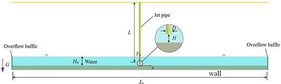
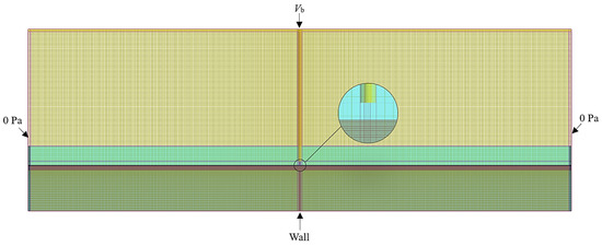
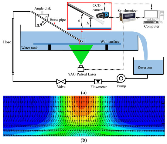
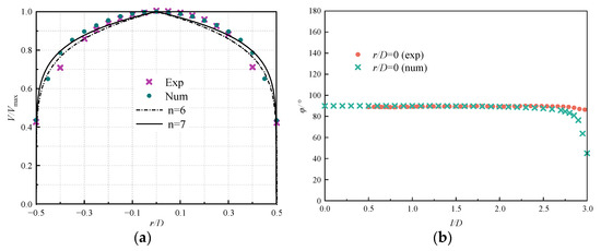
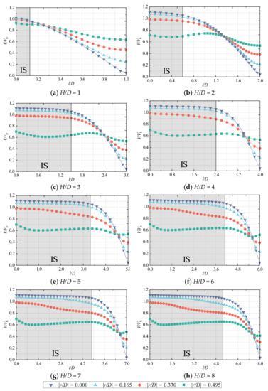
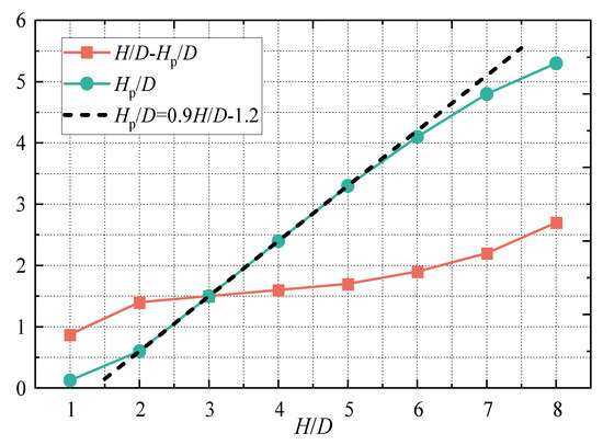
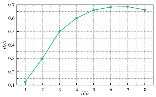
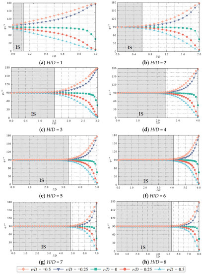
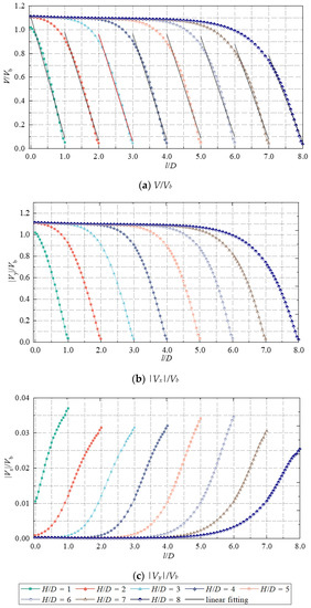
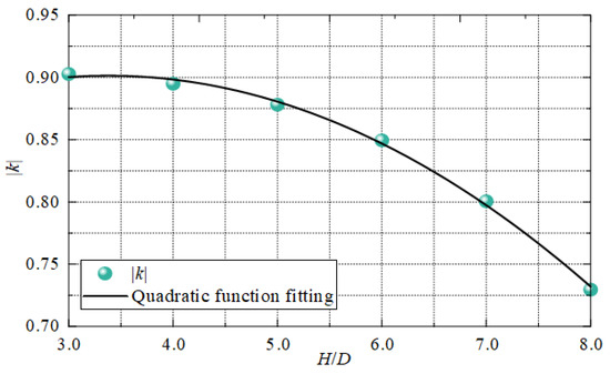
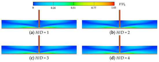
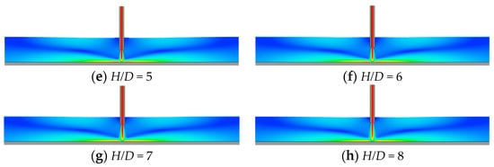
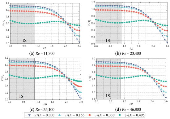
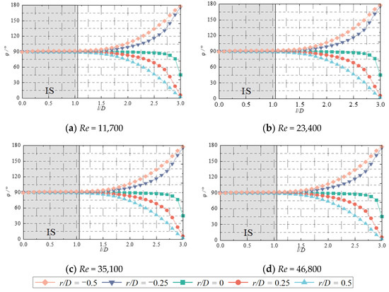
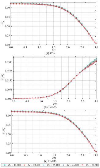
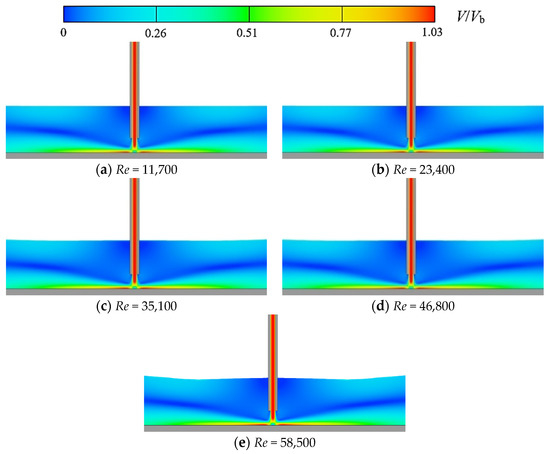


![Figure 2: Experimental data on height of
vertex formed [8] / Figure 3: Vertex height as a function of time](https://flow3d.co.kr/wp-content/uploads/Figure-3-Vertex-height-as-a-function-of-time-.png)


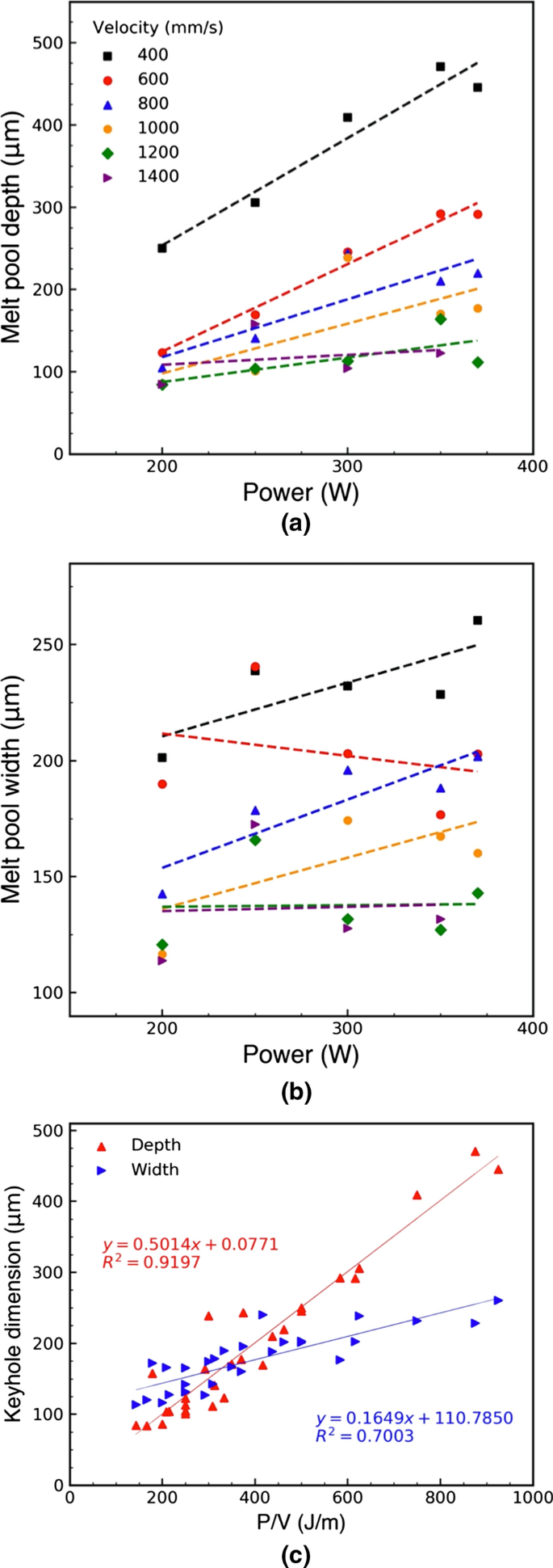
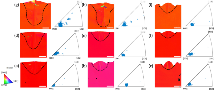
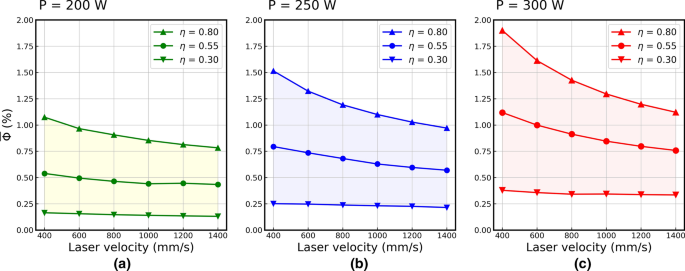
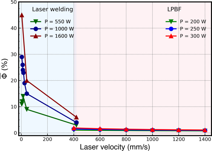
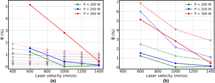
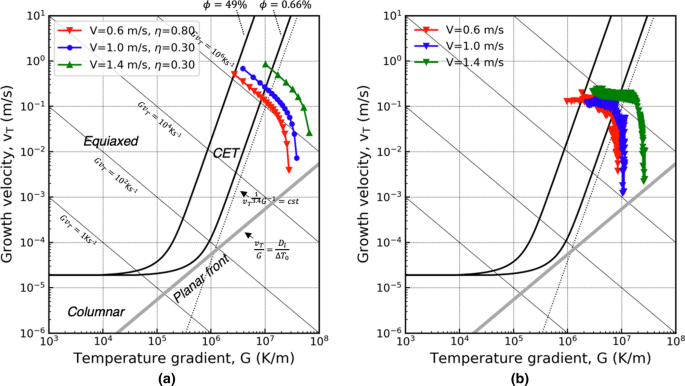
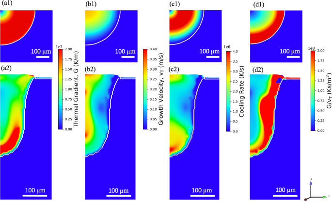
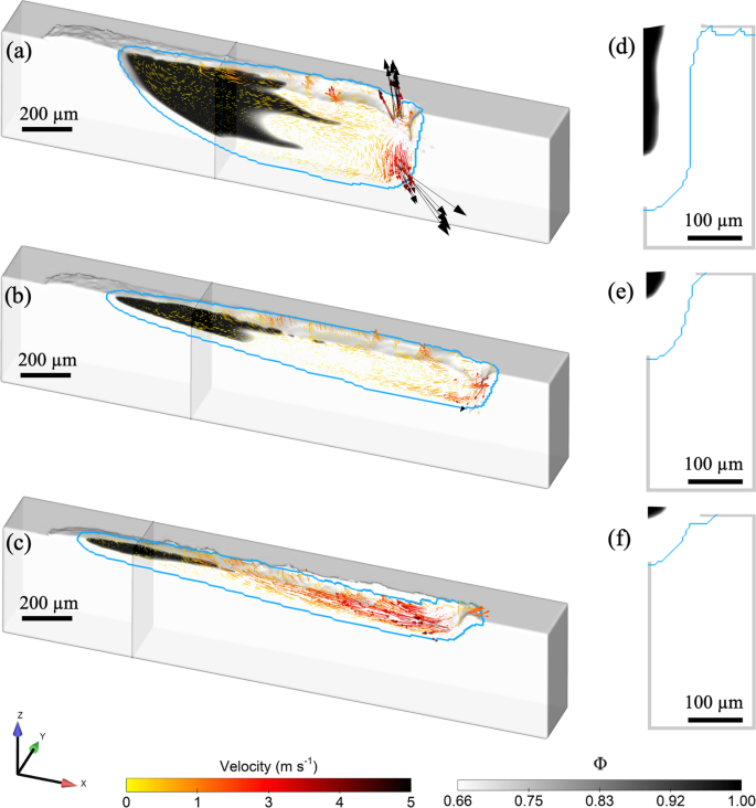


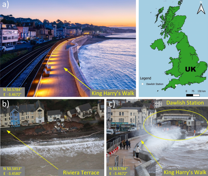
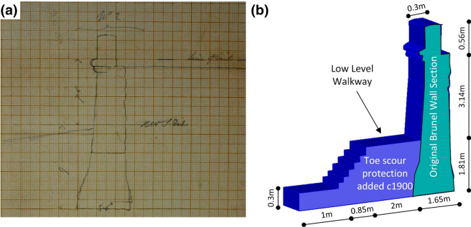
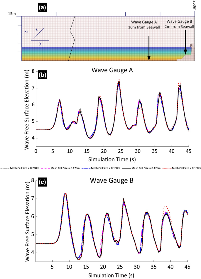
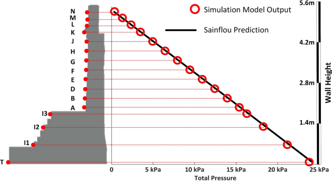
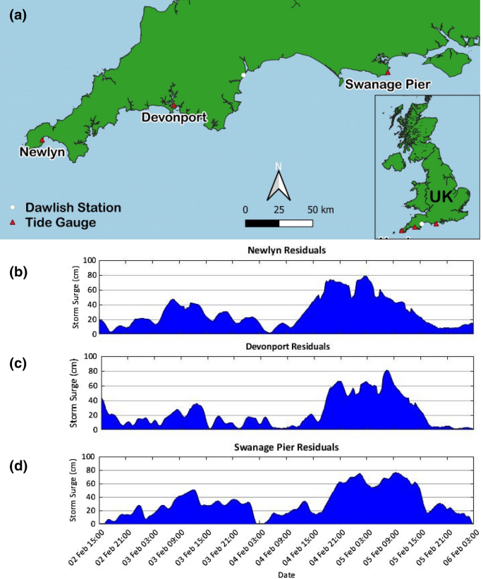
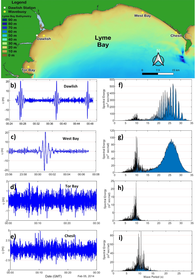
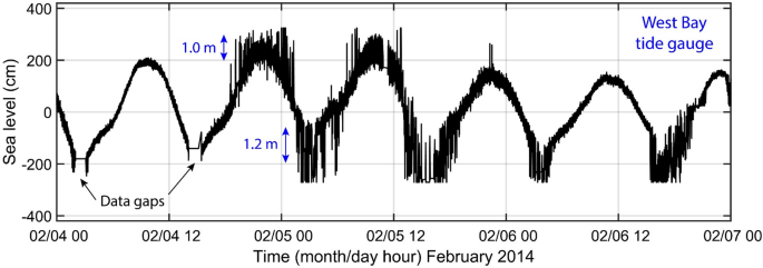
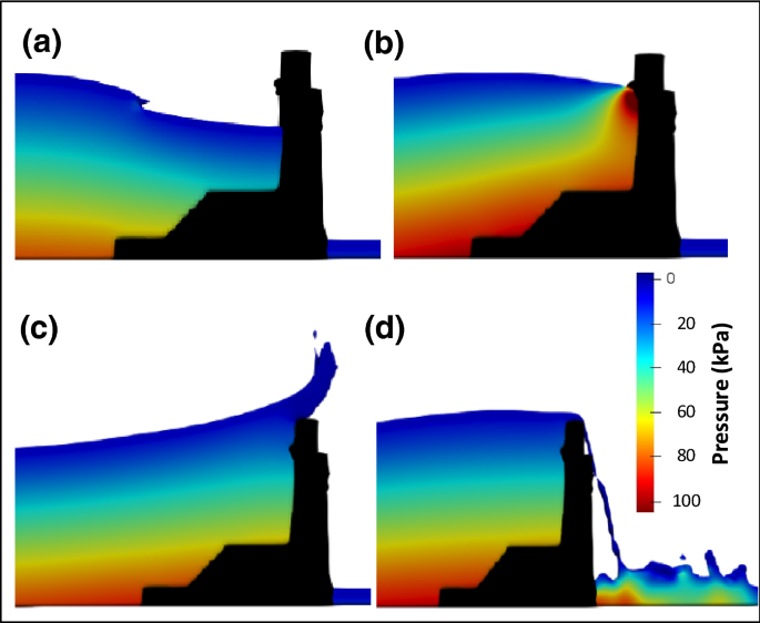
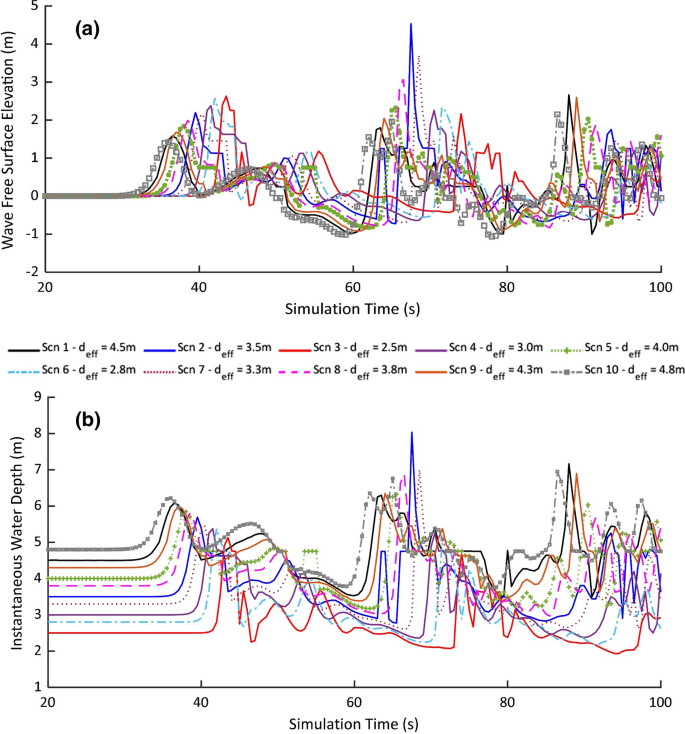
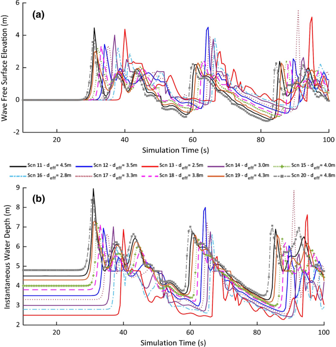
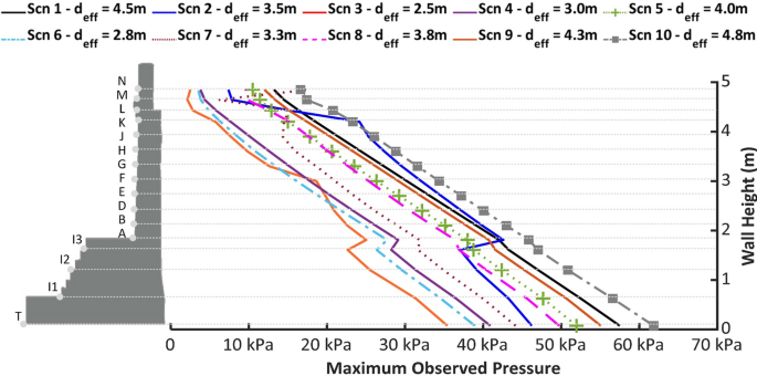
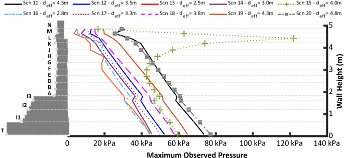
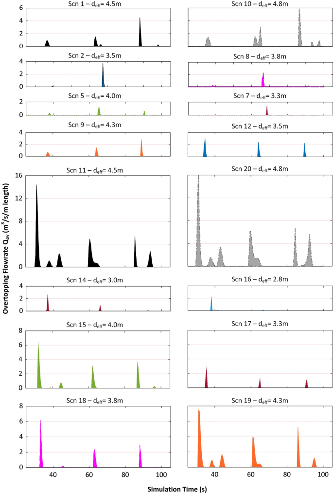
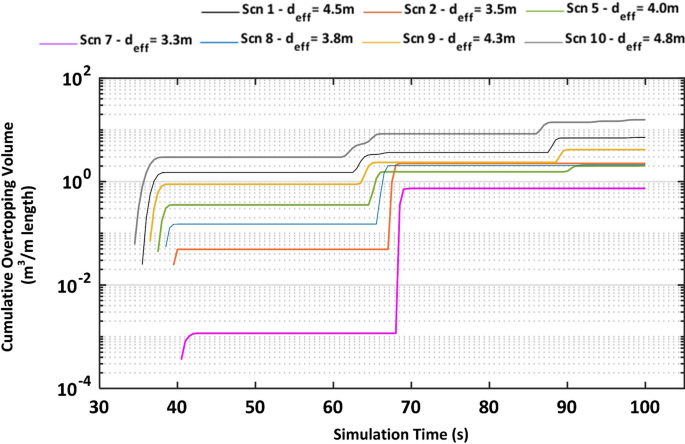
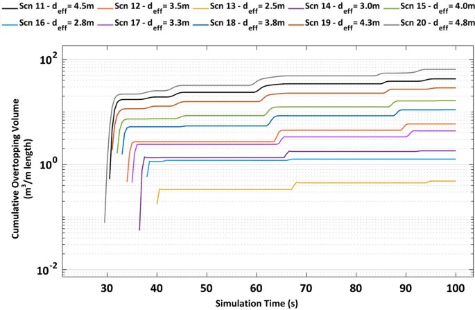







![Fig. 1. (a) Dimensions of the casting with runners (unit: mm), (b) a melt flow simulation using Flow-3D software together with Reilly's model[44], predicted that a large amount of bifilms (denoted by the black particles) would be contained in the final casting. (c) A solidification simulation using Pro-cast software showed that no shrinkage defect was contained in the final casting.](https://flow3d.co.kr/wp-content/uploads/Fig.-1.-a-Dimensions-of-the-casting-with-runners.png)
![Fig. 1. (a) Dimensions of the casting with runners (unit: mm), (b) a melt flow simulation using Flow-3D software together with Reilly's model[44], predicted that a large amount of bifilms (denoted by the black particles) would be contained in the final casting. (c) A solidification simulation using Pro-cast software showed that no shrinkage defect was contained in the final casting.](https://ars.els-cdn.com/content/image/1-s2.0-S2213956721001791-gr1_lrg.jpg)


![Fig. 3 2D melt pool contours from the numerical model compared to experiments [16] for (a) VED = 65 J/mm3 at 7 mm from the beginning of the single track (b) VED = 103 J/mm3 at 3 mm from the beginning of the single track (c) VED = 103 J/mm3 at 7 mm from the beginning of the single track. In the 2D contour, the non-melted region is indicated in blue, and the melted region is indicated by red and green when the VED is 65 J/mm3 and 103 J/mm3 respectively.](https://flow3d.co.kr/wp-content/uploads/Fig.-3-2D-melt-pool-contours-from-the-numerical-model-compared-to-experiments.png)