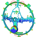
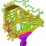
Figure 6. Evolution of melt pool in the overhang region (θ = 45°, P = 100 W, v = 1000 mm/s, the streamlines are shown by arrows).

Experimental and numerical investigation of the origin of surface roughness in laser powder bed fused overhang regions

레이저 파우더 베드 융합 오버행 영역에서 표면 거칠기의 원인에 대한 실험 및 수치 조사

Shaochuan Feng,Amar M. Kamat,Soheil Sabooni &Yutao PeiPages S66-S84 | Received 18 Jan 2021, Accepted 25 Feb 2021, Published online: 10 Mar 2021

ABSTRACT

Surface roughness of laser powder bed fusion (L-PBF) printed overhang regions is a major contributor to deteriorated shape accuracy/surface quality. This study investigates the mechanisms behind the evolution of surface roughness (Ra) in overhang regions. The evolution of surface morphology is the result of a combination of border track contour, powder adhesion, warp deformation, and dross formation, which is strongly related to the overhang angle (θ). When 0° ≤ θ ≤ 15°, the overhang angle does not affect Ra significantly since only a small area of the melt pool boundaries contacts the powder bed resulting in slight powder adhesion. When 15° < θ ≤ 50°, powder adhesion is enhanced by the melt pool sinking and the increased contact area between the melt pool boundary and powder bed. When θ > 50°, large waviness of the overhang contour, adhesion of powder clusters, severe warp deformation and dross formation increase Ra sharply.

레이저 파우더 베드 퓨전 (L-PBF) 프린팅 오버행 영역의 표면 거칠기는 형상 정확도 / 표면 품질 저하의 주요 원인입니다. 이 연구 는 오버행 영역에서 표면 거칠기 (Ra ) 의 진화 뒤에 있는 메커니즘을 조사합니다 . 표면 형태의 진화는 오버행 각도 ( θ ) 와 밀접한 관련이있는 경계 트랙 윤곽, 분말 접착, 뒤틀림 변형 및 드로스 형성의 조합의 결과입니다 . 0° ≤  θ  ≤ 15° 인 경우 , 용융풀 경계의 작은 영역 만 분말 베드와 접촉하여 약간의 분말 접착이 발생하기 때문에 오버행 각도가 R a에 큰 영향을 주지 않습니다 . 15° < θ 일 때  ≤ 50°, 용융 풀 싱킹 및 용융 풀 경계와 분말 베드 사이의 증가된 접촉 면적으로 분말 접착력이 향상됩니다. θ  > 50° 일 때 오버행 윤곽의 큰 파형, 분말 클러스터의 접착, 심한 휨 변형 및 드 로스 형성이 Ra 급격히 증가 합니다.

KEYWORDS: Laser powder bed fusion (L-PBF), melt pool dynamics, overhang region, shape deviation, surface roughness

1. Introduction

레이저 분말 베드 융합 (L-PBF)은 첨단 적층 제조 (AM) 기술로, 집중된 레이저 빔을 사용하여 금속 분말을 선택적으로 융합하여 슬라이스 된 3D 컴퓨터 지원에 따라 층별로 3 차원 (3D) 금속 부품을 구축합니다. 설계 (CAD) 모델 (Chatham, Long 및 Williams 2019 ; Tan, Zhu 및 Zhou 2020 ). 재료가 인쇄 층 아래에 ​​존재하는지 여부에 따라 인쇄 영역은 각각 솔리드 영역 또는 돌출 영역으로 분류 될 수 있습니다. 따라서 오버행 영역은 고체 기판이 아니라 분말 베드 바로 위에 건설되는 특수 구조입니다 (Patterson, Messimer 및 Farrington 2017). 오버행 영역은지지 구조를 포함하거나 포함하지 않고 구축 할 수 있으며, 지지대가있는 돌출 영역의 L-PBF는 지지체가 더 낮은 밀도로 구축된다는 점을 제외 하고 (Wang and Chou 2018 ) 고체 기판의 공정과 유사합니다 (따라서 기계적 강도가 낮기 때문에 L-PBF 공정 후 기계적으로 쉽게 제거 할 수 있습니다. 따라서지지 구조로 인쇄 된 오버행 영역은 L-PBF 공정 후 지지물 제거, 연삭 및 연마와 같은 추가 후 처리 단계가 필요합니다.

수평 내부 채널의 제작과 같은 일부 특정 경우에는 공정 후 지지대를 제거하기가 어려우므로 채널 상단 절반의 돌출부 영역을 지지대없이 건설해야합니다 (Hopkinson and Dickens 2000 ). 수평 내부 채널에 사용할 수없는지지 구조 외에도 내부 표면, 특히 등각 냉각 채널 (Feng, Kamat 및 Pei 2021 ) 에서 발생하는 복잡한 3D 채널 네트워크의 경우 표면 마감 프로세스를 구현하는 것도 어렵습니다 . 결과적으로 오버행 영역은 (i) 잔류 응력에 의한 변형, (ii) 계단 효과 (Kuo et al. 2020 ; Li et al. 2020 )로 인해 설계된 모양에서 벗어날 수 있습니다 .) 및 (iii) 원하지 않는 분말 소결로 인한 향상된 표면 거칠기; 여기서, 앞의 두 요소는 일반적으로 mm 길이 스케일에서 ‘매크로’편차로 분류되고 후자는 일반적으로 µm 길이 스케일에서 ‘마이크로’편차로 인식됩니다.

열 응력에 의한 변형은 오버행 영역에서 발생하는 중요한 문제입니다 (Patterson, Messimer 및 Farrington 2017 ). 국부적 인 용융 / 냉각은 용융 풀 내부 및 주변에서 큰 온도 구배를 유도하여 응고 된 층에 집중적 인 열 응력을 유발합니다. 열 응력에 의한 뒤틀림은 고체 영역을 현저하게 변형하지 않습니다. 이러한 영역은 아래의 여러 레이어에 의해 제한되기 때문입니다. 반면에 오버행 영역은 구속되지 않고 공정 중 응력 완화로 인해 상당한 변형이 발생합니다 (Kamat 및 Pei 2019 ). 더욱이 용융 깊이는 레이어 두께보다 큽니다 (이전 레이어도 재용 해되어 빌드 된 레이어간에 충분한 결합을 보장하기 때문입니다 [Yadroitsev et al. 2013 ; Kamath et al.2014 ]),응고 된 두께가 설계된 두께보다 크기 때문에형태 편차 (예 : 드 로스 [Charles et al. 2020 ; Feng et al. 2020 ])가 발생합니다. 마이크로 스케일에서 인쇄 된 표면 (R a 및 S a ∼ 10 μm)은 기계적으로 가공 된 표면보다 거칠다 (Duval-Chaneac et al. 2018 ; Wen et al. 2018 ). 이 문제는고형화 된 용융 풀의 가장자리에 부착 된 용융되지 않은 분말의 결과로 표면 거칠기 (R a )가 일반적으로 약 20 μm인 오버행 영역에서 특히 심각합니다 (Mazur et al. 2016 ; Pakkanen et al. 2016 ).

오버행 각도 ( θ , 빌드 방향과 관련하여 측정)는 오버행 영역의 뒤틀림 편향과 표면 거칠기에 영향을 미치는 중요한 매개 변수입니다 (Kamat and Pei 2019 ; Mingear et al. 2019 ). θ ∼ 45 ° 의 오버행 각도 는 일반적으로지지 구조없이 오버행 영역을 인쇄 할 수있는 임계 값으로 합의됩니다 (Pakkanen et al. 2016 ; Kadirgama et al. 2018 ). θ 일 때이 임계 값보다 크면 오버행 영역을 허용 가능한 표면 품질로 인쇄 할 수 없습니다. 오버행 각도 외에도 레이저 매개 변수 (레이저 에너지 밀도와 관련된)는 용융 풀의 모양 / 크기 및 용융 풀 역학에 영향을줌으로써 오버행 영역의 표면 거칠기에 영향을줍니다 (Wang et al. 2013 ; Mingear et al . 2019 ).

용융 풀 역학은 고체 (Shrestha 및 Chou 2018 ) 및 오버행 (Le et al. 2020 ) 영역 모두에서 수행되는 L-PBF 공정을 포함한 레이저 재료 가공의 일반적인 물리적 현상입니다 . 용융 풀 모양, 크기 및 냉각 속도는 잔류 응력으로 인한 변형과 ​​표면 거칠기에 모두 영향을 미치므로 처리 매개 변수와 표면 형태 / 품질 사이의 다리 역할을하며 용융 풀을 이해하기 위해 수치 시뮬레이션을 사용하여 추가 조사를 수행 할 수 있습니다. 거동과 표면 거칠기에 미치는 영향. 현재까지 고체 영역의 L-PBF 동안 용융 풀 동작을 시뮬레이션하기 위해 여러 연구가 수행되었습니다. 유한 요소 방법 (FEM)과 같은 시뮬레이션 기술 (Roberts et al. 2009 ; Du et al.2019 ), 유한 차분 법 (FDM) (Wu et al. 2018 ), 전산 유체 역학 (CFD) (Lee and Zhang 2016 ), 임의의 Lagrangian-Eulerian 방법 (ALE) (Khairallah and Anderson 2014 )을 사용하여 증발 반동 압력 (Hu et al. 2018 ) 및 Marangoni 대류 (Zhang et al. 2018 ) 현상을포함하는 열 전달 (온도 장) 및 물질 전달 (용융 흐름) 프로세스. 또한 이산 요소법 (DEM)을 사용하여 무작위 분산 분말 베드를 생성했습니다 (Lee and Zhang 2016 ; Wu et al. 2018 ). 이 모델은 분말 규모의 L-PBF 공정을 시뮬레이션했습니다 (Khairallah et al. 2016) 메조 스케일 (Khairallah 및 Anderson 2014 ), 단일 트랙 (Leitz et al. 2017 )에서 다중 트랙 (Foroozmehr et al. 2016 ) 및 다중 레이어 (Huang, Khamesee 및 Toyserkani 2019 )로.

그러나 결과적인 표면 거칠기를 결정하는 오버행 영역의 용융 풀 역학은 문헌에서 거의 관심을받지 못했습니다. 솔리드 영역의 L-PBF에 대한 기존 시뮬레이션 모델이 어느 정도 참조가 될 수 있지만 오버행 영역과 솔리드 영역 간의 용융 풀 역학에는 상당한 차이가 있습니다. 오버행 영역에서 용융 금속은 분말 입자 사이의 틈새로 아래로 흘러 용융 풀이 다공성 분말 베드가 제공하는 약한 지지체 아래로 가라 앉습니다. 이것은 중력과 표면 장력의 영향이 용융 풀의 결과적인 모양 / 크기를 결정하는 데 중요하며, 결과적으로 오버행 영역의 마이크로 스케일 형태의 진화에 중요합니다. 또한 분말 입자 사이의 공극, 열 조건 (예 : 에너지 흡수,2019 ; Karimi et al. 2020 ; 노래와 영 2020 ). 표면 거칠기는 (마이크로) 형상 편차를 증가시킬뿐만 아니라 주기적 하중 동안 미세 균열의 시작 지점 역할을함으로써 기계적 강도를 저하시킵니다 (Günther et al. 2018 ). 오버행 영역의 높은 표면 거칠기는 (마이크로) 정확도 / 품질에 대한 엄격한 요구 사항이있는 부품 제조에서 L-PBF의 적용을 제한합니다.

본 연구는 실험 및 시뮬레이션 연구를 사용하여 오버행 영역 (지지물없이 제작)의 미세 형상 편차 형성 메커니즘과 표면 거칠기의 기원을 체계적이고 포괄적으로 조사합니다. 결합 된 DEM-CFD 시뮬레이션 모델은 경계 트랙 윤곽, 분말 접착 및 뒤틀림 변형의 효과를 고려하여 오버행 영역의 용융 풀 역학과 표면 형태의 형성 메커니즘을 나타 내기 위해 개발되었습니다. 표면 거칠기 R의 시뮬레이션 및 단일 요인 L-PBF 인쇄 실험을 사용하여 오버행 각도의 함수로 연구됩니다. 용융 풀의 침몰과 관련된 오버행 영역에서 분말 접착의 세 가지 메커니즘이 식별되고 자세히 설명됩니다. 마지막으로, 인쇄 된 오버행 영역에서 높은 표면 거칠기 문제를 완화 할 수 있는 잠재적 솔루션에 대해 간략하게 설명합니다.

The shape and size of the L-PBF printed samples are illustrated in Figure 1
Figure 2. Borders in the overhang region depending on the overhang angle θ
Figure 3. (a) Profile of the volumetric heat source, (b) the model geometry of single-track printing on a solid substrate (unit: µm), and (c) the comparison of melt pool dimensions obtained from the experiment (right half) and simulation (left half) for a calibrated optical penetration depth of 110 µm (laser power 200 W and scan speed 800 mm/s, solidified layer thickness 30 µm, powder size 10–45 µm).
Figure 4. The model geometry of an overhang being L-PBF processed: (a) 3D view and (b) right view.
Figure 5. The cross-sectional contour of border tracks in a 45° overhang region.
Figure 6. Evolution of melt pool in the overhang region (θ = 45°, P = 100 W, v = 1000 mm/s, the streamlines are shown by arrows).
Figure 7. The overhang contour is contributed by (a) only outer borders when θ ≤ 60° (b) both inner borders and outer borders when θ > 60°.
Figure 8. Schematic of powder adhesion on a 45° overhang region.
Figure 9. The L-PBF printed samples with various overhang angle (a) θ = 0° (cube), (b) θ = 30°, (c) θ = 45°, (d) θ = 55° and (e) θ = 60°.
Figure 10. Two mechanisms of powder adhesion related to the overhang angle: (a) simulation-predicted, θ = 45°; (b) simulation-predicted, θ = 60°; (c, e) optical micrographs, θ = 45°; (d, f) optical micrographs, θ = 60°. (e) and (f) are partial enlargement of (c) and (d), respectively.
Figure 11. Simulation-predicted surface morphology in the overhang region at different overhang angle: (a) θ = 15°, (b) θ = 30°, (c) θ = 45°, (d) θ = 60° and (e) θ = 80° (Blue solid lines: simulation-predicted contour; red dashed lines: the planar profile of designed overhang region specified by the overhang angles).
Figure 12. Effect of overhang angle on surface roughness Ra in overhang regions
Figure 13. Surface morphology of L-PBF printed overhang regions with different overhang angle: (a) θ = 15°, (b) θ = 30°, (c) θ = 45° and (d) θ = 60° (overhang border parameters: P = 100 W, v = 1000 mm/s).
Figure 14. Effect of (a) laser power (scan speed = 1000 mm/s) and (b) scan speed (lase power = 100 W) on surface roughness Ra in overhang regions (θ = 45°, laser power and scan speed referred to overhang border parameters, and the other process parameters are listed in Table 2).

References

  • Cai, Chao, Chrupcala Radoslaw, Jinliang Zhang, Qian Yan, Shifeng Wen, Bo Song, and Yusheng Shi. 2019. “In-Situ Preparation and Formation of TiB/Ti-6Al-4V Nanocomposite via Laser Additive Manufacturing: Microstructure Evolution and Tribological Behavior.” Powder Technology 342: 73–84. doi:10.1016/j.powtec.2018.09.088. [Crossref], [Web of Science ®], [Google Scholar]
  • Cai, Chao, Wei Shian Tey, Jiayao Chen, Wei Zhu, Xingjian Liu, Tong Liu, Lihua Zhao, and Kun Zhou. 2021. “Comparative Study on 3D Printing of Polyamide 12 by Selective Laser Sintering and Multi Jet Fusion.” Journal of Materials Processing Technology 288 (August 2020): 116882. doi:10.1016/j.jmatprotec.2020.116882. [Crossref], [Web of Science ®], [Google Scholar]
  • Cai, Chao, Xu Wu, Wan Liu, Wei Zhu, Hui Chen, Jasper Dong Qiu Chua, Chen Nan Sun, Jie Liu, Qingsong Wei, and Yusheng Shi. 2020. “Selective Laser Melting of Near-α Titanium Alloy Ti-6Al-2Zr-1Mo-1V: Parameter Optimization, Heat Treatment and Mechanical Performance.” Journal of Materials Science and Technology 57: 51–64. doi:10.1016/j.jmst.2020.05.004. [Crossref], [Web of Science ®], [Google Scholar]
  • Charles, Amal, Ahmed Elkaseer, Lore Thijs, and Steffen G. Scholz. 2020. “Dimensional Errors Due to Overhanging Features in Laser Powder Bed Fusion Parts Made of Ti-6Al-4V.” Applied Sciences 10 (7): 2416. doi:10.3390/app10072416. [Crossref], [Google Scholar]
  • Chatham, Camden A., Timothy E. Long, and Christopher B. Williams. 2019. “A Review of the Process Physics and Material Screening Methods for Polymer Powder Bed Fusion Additive Manufacturing.” Progress in Polymer Science 93: 68–95. doi:10.1016/j.progpolymsci.2019.03.003. [Crossref], [Web of Science ®], [Google Scholar]
  • Du, Yang, Xinyu You, Fengbin Qiao, Lijie Guo, and Zhengwu Liu. 2019. “A Model for Predicting the Temperature Field during Selective Laser Melting.” Results in Physics 12 (November 2018): 52–60. doi:10.1016/j.rinp.2018.11.031. [Crossref], [Web of Science ®], [Google Scholar]
  • Duval-Chaneac, M. S., S. Han, C. Claudin, F. Salvatore, J. Bajolet, and J. Rech. 2018. “Experimental Study on Finishing of Internal Laser Melting (SLM) Surface with Abrasive Flow Machining (AFM).” Precision Engineering 54 (July 2017): 1–6. doi:10.1016/j.precisioneng.2018.03.006. [Crossref], [Web of Science ®], [Google Scholar]
  • Feng, Shaochuan, Shijie Chen, Amar M. Kamat, Ru Zhang, Mingji Huang, and Liangcai Hu. 2020. “Investigation on Shape Deviation of Horizontal Interior Circular Channels Fabricated by Laser Powder Bed Fusion.” Additive Manufacturing 36 (December): 101585. doi:10.1016/j.addma.2020.101585. [Crossref], [Web of Science ®], [Google Scholar]
  • Feng, Shaochuan, Chuanzhen Huang, Jun Wang, Hongtao Zhu, Peng Yao, and Zhanqiang Liu. 2017. “An Analytical Model for the Prediction of Temperature Distribution and Evolution in Hybrid Laser-Waterjet Micro-Machining.” Precision Engineering 47: 33–45. doi:10.1016/j.precisioneng.2016.07.002. [Crossref], [Web of Science ®], [Google Scholar]
  • Feng, Shaochuan, Amar M. Kamat, and Yutao Pei. 2021. “Design and Fabrication of Conformal Cooling Channels in Molds: Review and Progress Updates.” International Journal of Heat and Mass Transfer. doi:10.1016/j.ijheatmasstransfer.2021.121082. [Crossref], [PubMed], [Web of Science ®], [Google Scholar]
  • Flow-3D V11.2 Documentation. 2016. Flow Science, Inc. [Crossref], [Google Scholar]
  • Foroozmehr, Ali, Mohsen Badrossamay, Ehsan Foroozmehr, and Sa’id Golabi. 2016. “Finite Element Simulation of Selective Laser Melting Process Considering Optical Penetration Depth of Laser in Powder Bed.” Materials and Design 89: 255–263. doi:10.1016/j.matdes.2015.10.002. [Crossref], [Web of Science ®], [Google Scholar]
  • “Geometrical Product Specifications (GPS) — Surface Texture: Profile Method — Rules and Procedures for the Assessment of Surface Texture (ISO 4288).” 1996. International Organization for Standardization. https://www.iso.org/standard/2096.html. [Google Scholar]
  • Günther, Johannes, Stefan Leuders, Peter Koppa, Thomas Tröster, Sebastian Henkel, Horst Biermann, and Thomas Niendorf. 2018. “On the Effect of Internal Channels and Surface Roughness on the High-Cycle Fatigue Performance of Ti-6Al-4V Processed by SLM.” Materials & Design 143: 1–11. doi:10.1016/j.matdes.2018.01.042. [Crossref], [Web of Science ®], [Google Scholar]
  • Hopkinson, Neil, and Phill Dickens. 2000. “Conformal Cooling and Heating Channels Using Laser Sintered Tools.” In Solid Freeform Fabrication Conference, 490–497. Texas. doi:10.26153/tsw/3075. [Crossref], [Google Scholar]
  • Hu, Zhiheng, Haihong Zhu, Changchun Zhang, Hu Zhang, Ting Qi, and Xiaoyan Zeng. 2018. “Contact Angle Evolution during Selective Laser Melting.” Materials and Design 139: 304–313. doi:10.1016/j.matdes.2017.11.002. [Crossref], [Web of Science ®], [Google Scholar]
  • Hu, Cheng, Kejia Zhuang, Jian Weng, and Donglin Pu. 2019. “Three-Dimensional Analytical Modeling of Cutting Temperature for Round Insert Considering Semi-Infinite Boundary and Non-Uniform Heat Partition.” International Journal of Mechanical Sciences 155 (October 2018): 536–553. doi:10.1016/j.ijmecsci.2019.03.019. [Crossref], [Web of Science ®], [Google Scholar]
  • Huang, Yuze, Mir Behrad Khamesee, and Ehsan Toyserkani. 2019. “A New Physics-Based Model for Laser Directed Energy Deposition (Powder-Fed Additive Manufacturing): From Single-Track to Multi-Track and Multi-Layer.” Optics & Laser Technology 109 (August 2018): 584–599. doi:10.1016/j.optlastec.2018.08.015. [Crossref], [Web of Science ®], [Google Scholar]
  • Kadirgama, K., W. S. W. Harun, F. Tarlochan, M. Samykano, D. Ramasamy, Mohd Zaidi Azir, and H. Mehboob. 2018. “Statistical and Optimize of Lattice Structures with Selective Laser Melting (SLM) of Ti6AL4V Material.” International Journal of Advanced Manufacturing Technology 97 (1–4): 495–510. doi:10.1007/s00170-018-1913-1. [Crossref], [Web of Science ®], [Google Scholar]
  • Kamat, Amar M, and Yutao Pei. 2019. “An Analytical Method to Predict and Compensate for Residual Stress-Induced Deformation in Overhanging Regions of Internal Channels Fabricated Using Powder Bed Fusion.” Additive Manufacturing 29 (March): 100796. doi:10.1016/j.addma.2019.100796. [Crossref], [Web of Science ®], [Google Scholar]
  • Kamath, Chandrika, Bassem El-Dasher, Gilbert F. Gallegos, Wayne E. King, and Aaron Sisto. 2014. “Density of Additively-Manufactured, 316L SS Parts Using Laser Powder-Bed Fusion at Powers up to 400 W.” International Journal of Advanced Manufacturing Technology 74 (1–4): 65–78. doi:10.1007/s00170-014-5954-9. [Crossref], [Web of Science ®], [Google Scholar]
  • Karimi, J., C. Suryanarayana, I. Okulov, and K. G. Prashanth. 2020. “Selective Laser Melting of Ti6Al4V: Effect of Laser Re-Melting.” Materials Science and Engineering A (July): 140558. doi:10.1016/j.msea.2020.140558. [Crossref], [Web of Science ®], [Google Scholar]
  • Khairallah, Saad A., and Andy Anderson. 2014. “Mesoscopic Simulation Model of Selective Laser Melting of Stainless Steel Powder.” Journal of Materials Processing Technology 214 (11): 2627–2636. doi:10.1016/j.jmatprotec.2014.06.001. [Crossref], [Web of Science ®], [Google Scholar]
  • Khairallah, Saad A., Andrew T. Anderson, Alexander Rubenchik, and Wayne E. King. 2016. “Laser Powder-Bed Fusion Additive Manufacturing: Physics of Complex Melt Flow and Formation Mechanisms of Pores, Spatter, and Denudation Zones.” Edited by Adedeji B. Badiru, Vhance V. Valencia, and David Liu. Acta Materialia 108 (April): 36–45. doi:10.1016/j.actamat.2016.02.014. [Crossref], [Web of Science ®], [Google Scholar]
  • Kuo, C. N., C. K. Chua, P. C. Peng, Y. W. Chen, S. L. Sing, S. Huang, and Y. L. Su. 2020. “Microstructure Evolution and Mechanical Property Response via 3D Printing Parameter Development of Al–Sc Alloy.” Virtual and Physical Prototyping 15 (1): 120–129. doi:10.1080/17452759.2019.1698967. [Taylor & Francis Online], [Web of Science ®], [Google Scholar]
  • Le, K. Q., C. H. Wong, K. H. G. Chua, C. Tang, and H. Du. 2020. “Discontinuity of Overhanging Melt Track in Selective Laser Melting Process.” International Journal of Heat and Mass Transfer 162 (December): 120284. doi:10.1016/j.ijheatmasstransfer.2020.120284. [Crossref], [Web of Science ®], [Google Scholar]
  • Lee, Y. S., and W. Zhang. 2016. “Modeling of Heat Transfer, Fluid Flow and Solidification Microstructure of Nickel-Base Superalloy Fabricated by Laser Powder Bed Fusion.” Additive Manufacturing 12: 178–188. doi:10.1016/j.addma.2016.05.003. [Crossref], [Web of Science ®], [Google Scholar]
  • Leitz, K. H., P. Singer, A. Plankensteiner, B. Tabernig, H. Kestler, and L. S. Sigl. 2017. “Multi-Physical Simulation of Selective Laser Melting.” Metal Powder Report 72 (5): 331–338. doi:10.1016/j.mprp.2016.04.004. [Crossref], [Google Scholar]
  • Li, Jian, Jing Hu, Yi Zhu, Xiaowen Yu, Mengfei Yu, and Huayong Yang. 2020. “Surface Roughness Control of Root Analogue Dental Implants Fabricated Using Selective Laser Melting.” Additive Manufacturing 34 (September 2019): 101283. doi:10.1016/j.addma.2020.101283. [Crossref], [Web of Science ®], [Google Scholar]
  • Li, Yingli, Kun Zhou, Pengfei Tan, Shu Beng Tor, Chee Kai Chua, and Kah Fai Leong. 2018. “Modeling Temperature and Residual Stress Fields in Selective Laser Melting.” International Journal of Mechanical Sciences 136 (February): 24–35. doi:10.1016/j.ijmecsci.2017.12.001. [Crossref], [Web of Science ®], [Google Scholar]
  • Mazur, MacIej, Martin Leary, Matthew McMillan, Joe Elambasseril, and Milan Brandt. 2016. “SLM Additive Manufacture of H13 Tool Steel with Conformal Cooling and Structural Lattices.” Rapid Prototyping Journal 22 (3): 504–518. doi:10.1108/RPJ-06-2014-0075. [Crossref], [Web of Science ®], [Google Scholar]
  • Mingear, Jacob, Bing Zhang, Darren Hartl, and Alaa Elwany. 2019. “Effect of Process Parameters and Electropolishing on the Surface Roughness of Interior Channels in Additively Manufactured Nickel-Titanium Shape Memory Alloy Actuators.” Additive Manufacturing 27 (October 2018): 565–575. doi:10.1016/j.addma.2019.03.027. [Crossref], [Web of Science ®], [Google Scholar]
  • Pakkanen, Jukka, Flaviana Calignano, Francesco Trevisan, Massimo Lorusso, Elisa Paola Ambrosio, Diego Manfredi, and Paolo Fino. 2016. “Study of Internal Channel Surface Roughnesses Manufactured by Selective Laser Melting in Aluminum and Titanium Alloys.” Metallurgical and Materials Transactions A 47 (8): 3837–3844. doi:10.1007/s11661-016-3478-7. [Crossref], [Web of Science ®], [Google Scholar]
  • Patterson, Albert E., Sherri L. Messimer, and Phillip A. Farrington. 2017. “Overhanging Features and the SLM/DMLS Residual Stresses Problem: Review and Future Research Need.” Technologies 5 (4): 15. doi:10.3390/technologies5020015. [Crossref], [Web of Science ®], [Google Scholar]
  • Roberts, I. A., C. J. Wang, R. Esterlein, M. Stanford, and D. J. Mynors. 2009. “A Three-Dimensional Finite Element Analysis of the Temperature Field during Laser Melting of Metal Powders in Additive Layer Manufacturing.” International Journal of Machine Tools and Manufacture 49 (12–13): 916–923. doi:10.1016/j.ijmachtools.2009.07.004. [Crossref], [Web of Science ®], [Google Scholar]
  • Shrestha, Subin, and Kevin Chou. 2018. “Computational Analysis of Thermo-Fluid Dynamics with Metallic Powder in SLM.” In CFD Modeling and Simulation in Materials Processing 2018, edited by Laurentiu Nastac, Koulis Pericleous, Adrian S. Sabau, Lifeng Zhang, and Brian G. Thomas, 85–95. Cham, Switzerland: Springer Nature. doi:10.1007/978-3-319-72059-3_9. [Crossref], [Google Scholar]
  • Sing, S. L., and W. Y. Yeong. 2020. “Laser Powder Bed Fusion for Metal Additive Manufacturing: Perspectives on Recent Developments.” Virtual and Physical Prototyping 15 (3): 359–370. doi:10.1080/17452759.2020.1779999. [Taylor & Francis Online], [Web of Science ®], [Google Scholar]
  • Šmilauer, Václav, Emanuele Catalano, Bruno Chareyre, Sergei Dorofeenko, Jérôme Duriez, Nolan Dyck, Jan Eliáš, et al. 2015. Yade Documentation. 2nd ed. The Yade Project. doi:10.5281/zenodo.34073. [Crossref], [Google Scholar]
  • Tan, Pengfei, Fei Shen, Biao Li, and Kun Zhou. 2019. “A Thermo-Metallurgical-Mechanical Model for Selective Laser Melting of Ti6Al4V.” Materials & Design 168 (April): 107642. doi:10.1016/j.matdes.2019.107642. [Crossref], [Web of Science ®], [Google Scholar]
  • Tan, Lisa Jiaying, Wei Zhu, and Kun Zhou. 2020. “Recent Progress on Polymer Materials for Additive Manufacturing.” Advanced Functional Materials 30 (43): 1–54. doi:10.1002/adfm.202003062. [Crossref], [Web of Science ®], [Google Scholar]
  • Wang, Xiaoqing, and Kevin Chou. 2018. “Effect of Support Structures on Ti-6Al-4V Overhang Parts Fabricated by Powder Bed Fusion Electron Beam Additive Manufacturing.” Journal of Materials Processing Technology 257 (February): 65–78. doi:10.1016/j.jmatprotec.2018.02.038. [Crossref], [Web of Science ®], [Google Scholar]
  • Wang, Di, Yongqiang Yang, Ziheng Yi, and Xubin Su. 2013. “Research on the Fabricating Quality Optimization of the Overhanging Surface in SLM Process.” International Journal of Advanced Manufacturing Technology 65 (9–12): 1471–1484. doi:10.1007/s00170-012-4271-4. [Crossref], [Web of Science ®], [Google Scholar]
  • Wen, Peng, Maximilian Voshage, Lucas Jauer, Yanzhe Chen, Yu Qin, Reinhart Poprawe, and Johannes Henrich Schleifenbaum. 2018. “Laser Additive Manufacturing of Zn Metal Parts for Biodegradable Applications: Processing, Formation Quality and Mechanical Properties.” Materials and Design 155: 36–45. doi:10.1016/j.matdes.2018.05.057. [Crossref], [Web of Science ®], [Google Scholar]
  • Wu, Yu-che, Cheng-hung San, Chih-hsiang Chang, Huey-jiuan Lin, Raed Marwan, Shuhei Baba, and Weng-Sing Hwang. 2018. “Numerical Modeling of Melt-Pool Behavior in Selective Laser Melting with Random Powder Distribution and Experimental Validation.” Journal of Materials Processing Technology 254 (November 2017): 72–78. doi:10.1016/j.jmatprotec.2017.11.032. [Crossref], [Web of Science ®], [Google Scholar]
  • Yadroitsev, I., P. Krakhmalev, I. Yadroitsava, S. Johansson, and I. Smurov. 2013. “Energy Input Effect on Morphology and Microstructure of Selective Laser Melting Single Track from Metallic Powder.” Journal of Materials Processing Technology 213 (4): 606–613. doi:10.1016/j.jmatprotec.2012.11.014. [Crossref], [Web of Science ®], [Google Scholar]
  • Yu, Wenhui, Swee Leong Sing, Chee Kai Chua, and Xuelei Tian. 2019. “Influence of Re-Melting on Surface Roughness and Porosity of AlSi10Mg Parts Fabricated by Selective Laser Melting.” Journal of Alloys and Compounds 792: 574–581. doi:10.1016/j.jallcom.2019.04.017. [Crossref], [Web of Science ®], [Google Scholar]
  • Zhang, Dongyun, Pudan Zhang, Zhen Liu, Zhe Feng, Chengjie Wang, and Yanwu Guo. 2018. “Thermofluid Field of Molten Pool and Its Effects during Selective Laser Melting (SLM) of Inconel 718 Alloy.” Additive Manufacturing 21 (100): 567–578. doi:10.1016/j.addma.2018.03.031. [Crossref], [Web of Science ®], [Google Scholar]
Figure 1. (a) Top view of the microfluidic-magnetophoretic device, (b) Schematic representation of the channel cross-sections studied in this work, and (c) the magnet position relative to the channel location (Sepy and Sepz are the magnet separation distances in y and z, respectively).

Continuous-Flow Separation of Magnetic Particles from Biofluids: How Does the Microdevice Geometry Determine the Separation Performance?

1Department of Chemical and Biomolecular Engineering, ETSIIT, University of Cantabria, Avda. Los Castros s/n, 39005 Santander, Spain
2William G. Lowrie Department of Chemical and Biomolecular Engineering, The Ohio State University, 151 W. Woodruff Ave., Columbus, OH 43210, USA
*Author to whom correspondence should be addressed.
Sensors 202020(11), 3030; https://doi.org/10.3390/s20113030
Received: 16 April 2020 / Revised: 21 May 2020 / Accepted: 25 May 2020 / Published: 27 May 2020
(This article belongs to the Special Issue Lab-on-a-Chip and Microfluidic Sensors)

Abstract

The use of functionalized magnetic particles for the detection or separation of multiple chemicals and biomolecules from biofluids continues to attract significant attention. After their incubation with the targeted substances, the beads can be magnetically recovered to perform analysis or diagnostic tests. Particle recovery with permanent magnets in continuous-flow microdevices has gathered great attention in the last decade due to the multiple advantages of microfluidics. As such, great efforts have been made to determine the magnetic and fluidic conditions for achieving complete particle capture; however, less attention has been paid to the effect of the channel geometry on the system performance, although it is key for designing systems that simultaneously provide high particle recovery and flow rates. Herein, we address the optimization of Y-Y-shaped microchannels, where magnetic beads are separated from blood and collected into a buffer stream by applying an external magnetic field. The influence of several geometrical features (namely cross section shape, thickness, length, and volume) on both bead recovery and system throughput is studied. For that purpose, we employ an experimentally validated Computational Fluid Dynamics (CFD) numerical model that considers the dominant forces acting on the beads during separation. Our results indicate that rectangular, long devices display the best performance as they deliver high particle recovery and high throughput. Thus, this methodology could be applied to the rational design of lab-on-a-chip devices for any magnetically driven purification, enrichment or isolation.

Keywords: particle magnetophoresisCFDcross sectionchip fabrication

Korea Abstract

생체 유체에서 여러 화학 물질과 생체 분자의 검출 또는 분리를위한 기능화 된 자성 입자의 사용은 계속해서 상당한 관심을 받고 있습니다. 표적 물질과 함께 배양 한 후 비드를 자기 적으로 회수하여 분석 또는 진단 테스트를 수행 할 수 있습니다. 연속 흐름 마이크로 장치에서 영구 자석을 사용한 입자 회수는 마이크로 유체의 여러 장점으로 인해 지난 10 년 동안 큰 관심을 모았습니다. 

따라서 완전한 입자 포획을 달성하기 위한 자기 및 유체 조건을 결정하기 위해 많은 노력을 기울였습니다. 그러나 높은 입자 회수율과 유속을 동시에 제공하는 시스템을 설계하는 데있어 핵심이기는 하지만 시스템 성능에 대한 채널 형상의 영향에 대해서는 덜주의를 기울였습니다. 

여기에서 우리는 자기 비드가 혈액에서 분리되고 외부 자기장을 적용하여 버퍼 스트림으로 수집되는 YY 모양의 마이크로 채널의 최적화를 다룹니다. 비드 회수 및 시스템 처리량에 대한 여러 기하학적 특징 (즉, 단면 형상, 두께, 길이 및 부피)의 영향을 연구합니다. 

이를 위해 분리 중에 비드에 작용하는 지배적인 힘을 고려하는 실험적으로 검증 된 CFD (Computational Fluid Dynamics) 수치 모델을 사용합니다. 우리의 결과는 직사각형의 긴 장치가 높은 입자 회수율과 높은 처리량을 제공하기 때문에 최고의 성능을 보여줍니다. 

따라서 이 방법론은 자기 구동 정제, 농축 또는 분리를 위한 랩온어 칩 장치의 합리적인 설계에 적용될 수 있습니다.

Figure 1. (a) Top view of the microfluidic-magnetophoretic device, (b) Schematic representation of the channel cross-sections studied in this work, and (c) the magnet position relative to the channel location (Sepy and Sepz are the magnet separation distances in y and z, respectively).
Figure 2. (a) Channel-magnet configuration and (b–d) magnetic force distribution in the channel midplane for 2 mm, 5 mm and 10 mm long rectangular (left) and U-shaped (right) devices.
Figure 3. (a) Velocity distribution in a section perpendicular to the flow for rectangular (left) and U-shaped (right) cross section channels, and (b) particle location in these cross sections.
Figure 4. Influence of fluid flow rate on particle recovery when the applied magnetic force is (a) different and (b) equal in U-shaped and rectangular cross section microdevices.
Figure 5. Magnetic bead capture as a function of fluid flow rate for all of the studied geometries.
Figure 6. Influence of (a) magnetic and fluidic forces (J parameter) and (b) channel geometry (θ parameter) on particle recovery. Note that U-2mm does not accurately fit a line.
Figure 7. Dependence of bead capture on the (a) functional channel volume and (b) particle residence time (tres). Note that in the curve fitting expressions V represents the functional channel volume and that U-2mm does not accurately fit a line.

References

  1. Gómez-Pastora, J.; Xue, X.; Karampelas, I.H.; Bringas, E.; Furlani, E.P.; Ortiz, I. Analysis of separators for magnetic beads recovery: From large systems to multifunctional microdevices. Sep. Purif. Technol. 2017172, 16–31. [Google Scholar] [CrossRef]
  2. Wise, N.; Grob, T.; Morten, K.; Thompson, I.; Sheard, S. Magnetophoretic velocities of superparamagnetic particles, agglomerates and complexes. J. Magn. Magn. Mater. 2015384, 328–334. [Google Scholar] [CrossRef]
  3. Khashan, S.A.; Elnajjar, E.; Haik, Y. CFD simulation of the magnetophoretic separation in a microchannel. J. Magn. Magn. Mater. 2011323, 2960–2967. [Google Scholar] [CrossRef]
  4. Khashan, S.A.; Furlani, E.P. Scalability analysis of magnetic bead separation in a microchannel with an array of soft magnetic elements in a uniform magnetic field. Sep. Purif. Technol. 2014125, 311–318. [Google Scholar] [CrossRef]
  5. Furlani, E.P. Magnetic biotransport: Analysis and applications. Materials 20103, 2412–2446. [Google Scholar] [CrossRef]
  6. Gómez-Pastora, J.; Bringas, E.; Ortiz, I. Design of novel adsorption processes for the removal of arsenic from polluted groundwater employing functionalized magnetic nanoparticles. Chem. Eng. Trans. 201647, 241–246. [Google Scholar]
  7. Gómez-Pastora, J.; Bringas, E.; Lázaro-Díez, M.; Ramos-Vivas, J.; Ortiz, I. The reverse of controlled release: Controlled sequestration of species and biotoxins into nanoparticles (NPs). In Drug Delivery Systems; Stroeve, P., Mahmoudi, M., Eds.; World Scientific: Hackensack, NJ, USA, 2017; pp. 207–244. ISBN 9789813201057. [Google Scholar]
  8. Ruffert, C. Magnetic bead-magic bullet. Micromachines 20167, 21. [Google Scholar] [CrossRef]
  9. Yáñez-Sedeño, P.; Campuzano, S.; Pingarrón, J.M. Magnetic particles coupled to disposable screen printed transducers for electrochemical biosensing. Sensors 201616, 1585. [Google Scholar] [CrossRef]
  10. Schrittwieser, S.; Pelaz, B.; Parak, W.J.; Lentijo-Mozo, S.; Soulantica, K.; Dieckhoff, J.; Ludwig, F.; Guenther, A.; Tschöpe, A.; Schotter, J. Homogeneous biosensing based on magnetic particle labels. Sensors 201616, 828. [Google Scholar] [CrossRef]

  11. He, J.; Huang, M.; Wang, D.; Zhang, Z.; Li, G. Magnetic separation techniques in sample preparation for biological analysis: A review. J. Pharm. Biomed. Anal. 2014101, 84–101. [Google Scholar] [CrossRef]
  12. Ha, Y.; Ko, S.; Kim, I.; Huang, Y.; Mohanty, K.; Huh, C.; Maynard, J.A. Recent advances incorporating superparamagnetic nanoparticles into immunoassays. ACS Appl. Nano Mater. 20181, 512–521. [Google Scholar] [CrossRef]
  13. Gómez-Pastora, J.; González-Fernández, C.; Fallanza, M.; Bringas, E.; Ortiz, I. Flow patterns and mass transfer performance of miscible liquid-liquid flows in various microchannels: Numerical and experimental studies. Chem. Eng. J. 2018344, 487–497. [Google Scholar] [CrossRef]
  14. Gale, B.K.; Jafek, A.R.; Lambert, C.J.; Goenner, B.L.; Moghimifam, H.; Nze, U.C.; Kamarapu, S.K. A review of current methods in microfluidic device fabrication and future commercialization prospects. Inventions 20183, 60. [Google Scholar] [CrossRef]
  15. Nanobiotechnology; Concepts, Applications and Perspectives; Niemeyer, C.M.; Mirkin, C.A. (Eds.) Wiley-VCH: Weinheim, Germany, 2004; ISBN 3527305068. [Google Scholar]
  16. Khashan, S.A.; Dagher, S.; Alazzam, A.; Mathew, B.; Hilal-Alnaqbi, A. Microdevice for continuous flow magnetic separation for bioengineering applications. J. Micromech. Microeng. 201727, 055016. [Google Scholar] [CrossRef]
  17. Basauri, A.; Gomez-Pastora, J.; Fallanza, M.; Bringas, E.; Ortiz, I. Predictive model for the design of reactive micro-separations. Sep. Purif. Technol. 2019209, 900–907. [Google Scholar] [CrossRef]
  18. Abdollahi, P.; Karimi-Sabet, J.; Moosavian, M.A.; Amini, Y. Microfluidic solvent extraction of calcium: Modeling and optimization of the process variables. Sep. Purif. Technol. 2020231, 115875. [Google Scholar] [CrossRef]
  19. Khashan, S.A.; Alazzam, A.; Furlani, E. A novel design for a microfluidic magnetophoresis system: Computational study. In Proceedings of the 12th International Symposium on Fluid Control, Measurement and Visualization (FLUCOME2013), Nara, Japan, 18–23 November 2013. [Google Scholar]
  20. Pamme, N. Magnetism and microfluidics. Lab Chip 20066, 24–38. [Google Scholar] [CrossRef]
  21. Gómez-Pastora, J.; Amiri Roodan, V.; Karampelas, I.H.; Alorabi, A.Q.; Tarn, M.D.; Iles, A.; Bringas, E.; Paunov, V.N.; Pamme, N.; Furlani, E.P.; et al. Two-step numerical approach to predict ferrofluid droplet generation and manipulation inside multilaminar flow chambers. J. Phys. Chem. C 2019123, 10065–10080. [Google Scholar] [CrossRef]
  22. Gómez-Pastora, J.; Karampelas, I.H.; Bringas, E.; Furlani, E.P.; Ortiz, I. Numerical analysis of bead magnetophoresis from flowing blood in a continuous-flow microchannel: Implications to the bead-fluid interactions. Sci. Rep. 20199, 7265. [Google Scholar] [CrossRef]
  23. Tarn, M.D.; Pamme, N. On-Chip Magnetic Particle-Based Immunoassays Using Multilaminar Flow for Clinical Diagnostics. In Microchip Diagnostics Methods and Protocols; Taly, V., Viovy, J.L., Descroix, S., Eds.; Humana Press: New York, NY, USA, 2017; pp. 69–83. [Google Scholar]
  24. Phurimsak, C.; Tarn, M.D.; Peyman, S.A.; Greenman, J.; Pamme, N. On-chip determination of c-reactive protein using magnetic particles in continuous flow. Anal. Chem. 201486, 10552–10559. [Google Scholar] [CrossRef]
  25. Wu, X.; Wu, H.; Hu, Y. Enhancement of separation efficiency on continuous magnetophoresis by utilizing L/T-shaped microchannels. Microfluid. Nanofluid. 201111, 11–24. [Google Scholar] [CrossRef]
  26. Vojtíšek, M.; Tarn, M.D.; Hirota, N.; Pamme, N. Microfluidic devices in superconducting magnets: On-chip free-flow diamagnetophoresis of polymer particles and bubbles. Microfluid. Nanofluid. 201213, 625–635. [Google Scholar] [CrossRef]
  27. Gómez-Pastora, J.; González-Fernández, C.; Real, E.; Iles, A.; Bringas, E.; Furlani, E.P.; Ortiz, I. Computational modeling and fluorescence microscopy characterization of a two-phase magnetophoretic microsystem for continuous-flow blood detoxification. Lab Chip 201818, 1593–1606. [Google Scholar] [CrossRef] [PubMed]
  28. Forbes, T.P.; Forry, S.P. Microfluidic magnetophoretic separations of immunomagnetically labeled rare mammalian cells. Lab Chip 201212, 1471–1479. [Google Scholar] [CrossRef]
  29. Nandy, K.; Chaudhuri, S.; Ganguly, R.; Puri, I.K. Analytical model for the magnetophoretic capture of magnetic microspheres in microfluidic devices. J. Magn. Magn. Mater. 2008320, 1398–1405. [Google Scholar] [CrossRef]
  30. Plouffe, B.D.; Lewis, L.H.; Murthy, S.K. Computational design optimization for microfluidic magnetophoresis. Biomicrofluidics 20115, 013413. [Google Scholar] [CrossRef] [PubMed]
  31. Hale, C.; Darabi, J. Magnetophoretic-based microfluidic device for DNA isolation. Biomicrofluidics 20148, 044118. [Google Scholar] [CrossRef] [PubMed]
  32. Becker, H.; Gärtner, C. Polymer microfabrication methods for microfluidic analytical applications. Electrophoresis 200021, 12–26. [Google Scholar] [CrossRef]
  33. Pekas, N.; Zhang, Q.; Nannini, M.; Juncker, D. Wet-etching of structures with straight facets and adjustable taper into glass substrates. Lab Chip 201010, 494–498. [Google Scholar] [CrossRef]
  34. Wang, T.; Chen, J.; Zhou, T.; Song, L. Fabricating microstructures on glass for microfluidic chips by glass molding process. Micromachines 20189, 269. [Google Scholar] [CrossRef]
  35. Castaño-Álvarez, M.; Pozo Ayuso, D.F.; García Granda, M.; Fernández-Abedul, M.T.; Rodríguez García, J.; Costa-García, A. Critical points in the fabrication of microfluidic devices on glass substrates. Sens. Actuators B Chem. 2008130, 436–448. [Google Scholar] [CrossRef]
  36. Prakash, S.; Kumar, S. Fabrication of microchannels: A review. Proc. Inst. Mech. Eng. Part B J. Eng. Manuf. 2015229, 1273–1288. [Google Scholar] [CrossRef]
  37. Leester-Schädel, M.; Lorenz, T.; Jürgens, F.; Ritcher, C. Fabrication of Microfluidic Devices. In Microsystems for Pharmatechnology: Manipulation of Fluids, Particles, Droplets, and Cells; Dietzel, A., Ed.; Springer: Basel, Switzerland, 2016; pp. 23–57. ISBN 9783319269207. [Google Scholar]
  38. Bartlett, N.W.; Wood, R.J. Comparative analysis of fabrication methods for achieving rounded microchannels in PDMS. J. Micromech. Microeng. 201626, 115013. [Google Scholar] [CrossRef]
  39. Ng, P.F.; Lee, K.I.; Yang, M.; Fei, B. Fabrication of 3D PDMS microchannels of adjustable cross-sections via versatile gel templates. Polymers 201911, 64. [Google Scholar] [CrossRef] [PubMed]
  40. Furlani, E.P.; Sahoo, Y.; Ng, K.C.; Wortman, J.C.; Monk, T.E. A model for predicting magnetic particle capture in a microfluidic bioseparator. Biomed. Microdevices 20079, 451–463. [Google Scholar] [CrossRef]
  41. Tarn, M.D.; Peyman, S.A.; Robert, D.; Iles, A.; Wilhelm, C.; Pamme, N. The importance of particle type selection and temperature control for on-chip free-flow magnetophoresis. J. Magn. Magn. Mater. 2009321, 4115–4122. [Google Scholar] [CrossRef]
  42. Furlani, E.P. Permanent Magnet and Electromechanical Devices; Materials, Analysis and Applications; Academic Press: Waltham, MA, USA, 2001. [Google Scholar]
  43. White, F.M. Viscous Fluid Flow; McGraw-Hill: New York, NY, USA, 1974. [Google Scholar]
  44. Mathew, B.; Alazzam, A.; El-Khasawneh, B.; Maalouf, M.; Destgeer, G.; Sung, H.J. Model for tracing the path of microparticles in continuous flow microfluidic devices for 2D focusing via standing acoustic waves. Sep. Purif. Technol. 2015153, 99–107. [Google Scholar] [CrossRef]
  45. Furlani, E.J.; Furlani, E.P. A model for predicting magnetic targeting of multifunctional particles in the microvasculature. J. Magn. Magn. Mater. 2007312, 187–193. [Google Scholar] [CrossRef]
  46. Furlani, E.P.; Ng, K.C. Analytical model of magnetic nanoparticle transport and capture in the microvasculature. Phys. Rev. E 200673, 061919. [Google Scholar] [CrossRef]
  47. Eibl, R.; Eibl, D.; Pörtner, R.; Catapano, G.; Czermak, P. Cell and Tissue Reaction Engineering; Springer: Berlin/Heidelberg, Germany, 2009. [Google Scholar]
  48. Pamme, N.; Eijkel, J.C.T.; Manz, A. On-chip free-flow magnetophoresis: Separation and detection of mixtures of magnetic particles in continuous flow. J. Magn. Magn. Mater. 2006307, 237–244. [Google Scholar] [CrossRef]
  49. Alorabi, A.Q.; Tarn, M.D.; Gómez-Pastora, J.; Bringas, E.; Ortiz, I.; Paunov, V.N.; Pamme, N. On-chip polyelectrolyte coating onto magnetic droplets-Towards continuous flow assembly of drug delivery capsules. Lab Chip 201717, 3785–3795. [Google Scholar] [CrossRef]
  50. Zhang, H.; Guo, H.; Chen, Z.; Zhang, G.; Li, Z. Application of PECVD SiC in glass micromachining. J. Micromech. Microeng. 200717, 775–780. [Google Scholar] [CrossRef]
  51. Mourzina, Y.; Steffen, A.; Offenhäusser, A. The evaporated metal masks for chemical glass etching for BioMEMS. Microsyst. Technol. 200511, 135–140. [Google Scholar] [CrossRef]
  52. Mata, A.; Fleischman, A.J.; Roy, S. Fabrication of multi-layer SU-8 microstructures. J. Micromech. Microeng. 200616, 276–284. [Google Scholar] [CrossRef]
  53. Su, N. 8 2000 Negative Tone Photoresist Formulations 2002–2025; MicroChem Corporation: Newton, MA, USA, 2002. [Google Scholar]
  54. Su, N. 8 2000 Negative Tone Photoresist Formulations 2035–2100; MicroChem Corporation: Newton, MA, USA, 2002. [Google Scholar]
  55. Fu, C.; Hung, C.; Huang, H. A novel and simple fabrication method of embedded SU-8 micro channels by direct UV lithography. J. Phys. Conf. Ser. 200634, 330–335. [Google Scholar] [CrossRef]
  56. Kazoe, Y.; Yamashiro, I.; Mawatari, K.; Kitamori, T. High-pressure acceleration of nanoliter droplets in the gas phase in a microchannel. Micromachines 20167, 142. [Google Scholar] [CrossRef]
  57. Sharp, K.V.; Adrian, R.J.; Santiago, J.G.; Molho, J.I. Liquid flows in microchannels. In MEMS: Introduction and Fundamentals; Gad-el-Hak, M., Ed.; CRC Press: Boca Raton, FL, USA, 2006; pp. 10-1–10-46. ISBN 9781420036572. [Google Scholar]
  58. Oh, K.W.; Lee, K.; Ahn, B.; Furlani, E.P. Design of pressure-driven microfluidic networks using electric circuit analogy. Lab Chip 201212, 515–545. [Google Scholar] [CrossRef]
  59. Bruus, H. Theoretical Microfluidics; Oxford University Press: New York, NY, USA, 2008; ISBN 9788578110796. [Google Scholar]
  60. Beebe, D.J.; Mensing, G.A.; Walker, G.M. Physics and applications of microfluidics in biology. Annu. Rev. Biomed. Eng. 20024, 261–286. [Google Scholar] [CrossRef] [PubMed]
  61. Yalikun, Y.; Tanaka, Y. Large-scale integration of all-glass valves on a microfluidic device. Micromachines 20167, 83. [Google Scholar] [CrossRef] [PubMed]
  62. Van Heeren, H.; Verhoeven, D.; Atkins, T.; Tzannis, A.; Becker, H.; Beusink, W.; Chen, P. Design Guideline for Microfluidic Device and Component Interfaces (Part 2), Version 3; Available online: http://www.makefluidics.com/en/design-guideline?id=7 (accessed on 9 March 2020).
  63. Scheuble, N.; Iles, A.; Wootton, R.C.R.; Windhab, E.J.; Fischer, P.; Elvira, K.S. Microfluidic technique for the simultaneous quantification of emulsion instabilities and lipid digestion kinetics. Anal. Chem. 201789, 9116–9123. [Google Scholar] [CrossRef] [PubMed]
  64. Lynch, E.C. Red blood cell damage by shear stress. Biophys. J. 197212, 257–273. [Google Scholar]
  65. Paul, R.; Apel, J.; Klaus, S.; Schügner, F.; Schwindke, P.; Reul, H. Shear stress related blood damage in laminar Couette flow. Artif. Organs 200327, 517–529. [Google Scholar] [CrossRef] [PubMed]
  66. Gómez-Pastora, J.; Karampelas, I.H.; Xue, X.; Bringas, E.; Furlani, E.P.; Ortiz, I. Magnetic bead separation from flowing blood in a two-phase continuous-flow magnetophoretic microdevice: Theoretical analysis through computational fluid dynamics simulation. J. Phys. Chem. C 2017121, 7466–7477. [Google Scholar] [CrossRef]
  67. Lim, J.; Yeap, S.P.; Leow, C.H.; Toh, P.Y.; Low, S.C. Magnetophoresis of iron oxide nanoparticles at low field gradient: The role of shape anisotropy. J. Colloid Interface Sci. 2014421, 170–177. [Google Scholar] [CrossRef] [PubMed]
  68. Culbertson, C.T.; Sibbitts, J.; Sellens, K.; Jia, S. Fabrication of Glass Microfluidic Devices. In Microfluidic Electrophoresis: Methods and Protocols; Dutta, D., Ed.; Humana Press: New York, NY, USA, 2019; pp. 1–12. ISBN 978-1-4939-8963-8. [Google Scholar]
Fluid velocity magnitude including velocity vectors and blood volumetric fraction contours for scenario 3: (a,b) Magnet distance d = 0; (c,d) Magnet distance d = 1 mm.

Numerical Analysis of Bead Magnetophoresis from Flowing Blood in a Continuous-Flow Microchannel: Implications to the Bead-Fluid Interactions

Scientific Reports volume 9, Article number: 7265 (2019) Cite this article

Abstract

이 연구에서는 비드 운동과 유체 흐름에 미치는 영향에 대한 자세한 분석을 제공하기 위해 연속 흐름 마이크로 채널 내부의 비드 자기 영동에 대한 수치 흐름 중심 연구를 보고합니다.

수치 모델은 Lagrangian 접근 방식을 포함하며 영구 자석에 의해 생성 된 자기장의 적용에 의해 혈액에서 비드 분리 및 유동 버퍼로의 수집을 예측합니다.

다음 시나리오가 모델링됩니다. (i) 운동량이 유체에서 점 입자로 처리되는 비드로 전달되는 단방향 커플 링, (ii) 비드가 점 입자로 처리되고 운동량이 다음으로부터 전달되는 양방향 결합 비드를 유체로 또는 그 반대로, (iii) 유체 변위에서 비드 체적의 영향을 고려한 양방향 커플 링.

결과는 세 가지 시나리오에서 비드 궤적에 약간의 차이가 있지만 특히 높은 자기력이 비드에 적용될 때 유동장에 상당한 변화가 있음을 나타냅니다.

따라서 높은 자기력을 사용할 때 비드 운동과 유동장의 체적 효과를 고려한 정확한 전체 유동 중심 모델을 해결해야 합니다. 그럼에도 불구하고 비드가 중간 또는 낮은 자기력을 받을 때 계산적으로 저렴한 모델을 안전하게 사용하여 자기 영동을 모델링 할 수 있습니다.

Sketch of the magnetophoresis process in the continuous-flow microdevice.
Schematic view of the microdevice showing the working conditions set in the simulations.
Bead trajectories for different magnetic field conditions, magnet placed at different distances “d” from the channel: (a) d = 0; (b) d = 1 mm; (c) d = 1.5 mm; (d) d = 2 mm
Separation efficacy as a function of the magnet distance. Comparison between one-way and two-way coupling.
(a) Fluid velocity magnitude including velocity vectors and (b) blood volumetric fraction contours with magnet distance d = 0 mm for scenario 1 (t = 0.25 s).
luid velocity magnitude including velocity vectors and blood volumetric fraction contours for scenario 2: (a,b) Magnet distance d = 0 mm at t = 0.4 s; (c,d) Magnet distance d = 1 mm at t = 0.4 s.
Fluid velocity magnitude including velocity vectors and blood volumetric fraction contours for scenario 3: (a,b) Magnet distance d = 0; (c,d) Magnet distance d = 1 mm.
Blood volumetric fraction contours. Scenario 1: (a) Magnet distance d = 0 and (b) Magnet distance d = 1 mm; Scenario 2: (c) Magnet distance d = 0 and (d) Magnet distance d = 1 mm; and Scenario 3: (e) Magnet distance d = 0 and (f) Magnet distance d = 1 mm.

References

  1. 1.Keshipour, S. & Khalteh, N. K. Oxidation of ethylbenzene to styrene oxide in the presence of cellulose-supported Pd magnetic nanoparticles. Appl. Organometal. Chem. 30, 653–656 (2016).CAS Article Google Scholar 
  2. 2.Neamtu, M. et al. Functionalized magnetic nanoparticles: synthesis, characterization, catalytic application and assessment of toxicity. Sci. Rep. 8(1), 6278 (2018).ADS MathSciNet Article Google Scholar 
  3. 3.Gómez-Pastora, J., Bringas, E. & Ortiz, I. Recent progress and future challenges on the use of high performance magnetic nano-adsorbents in environmental applications. Chem. Eng. J. 256, 187–204 (2014).Article Google Scholar 
  4. 4.Gómez-Pastora, J., Bringas, E. & Ortiz, I. Design of novel adsorption processes for the removal of arsenic from polluted groundwater employing functionalized magnetic nanoparticles. Chem. Eng. Trans. 47, 241–246 (2016).Google Scholar 
  5. 5.Bagbi, Y., Sarswat, A., Mohan, D., Pandey, A. & Solanki, P. R. Lead and chromium adsorption from water using L-Cysteine functionalized magnetite (Fe3O4) nanoparticles. Sci. Rep. 7(1), 7672 (2017).ADS Article Google Scholar 
  6. 6.Gómez-Pastora, J. et al. Review and perspectives on the use of magnetic nanophotocatalysts (MNPCs) in water treatment. Chem. Eng. J. 310, 407–427 (2017).Article Google Scholar 
  7. 7.Lee, H. Y. et al. A selective fluoroionophore based on BODIPY-functionalized magnetic silica nanoparticles: removal of Pb2+ from human blood. Angew. Chem. Int. Ed. 48, 1239–1243 (2009).CAS Article Google Scholar 
  8. 8.Buzea, C., Pacheco, I. I. & Robbie, K. Nanomaterials and nanoparticles: sources and toxicity. Biointerphases 2, MR17–MR71 (2007).Article Google Scholar 
  9. 9.Roux, S. et al. Multifunctional nanoparticles: from the detection of biomolecules to the therapy. Int. J. Nanotechnol. 7, 781–801 (2010).ADS CAS Article Google Scholar 
  10. 10.Gómez-Pastora, J., Bringas, E., Lázaro-Díez, M., Ramos-Vivas, J. & Ortiz, I. In Drug Delivery Systems (Stroeve, P. & Mahmoudi, M. ed) 207–244 (World Scientific, 2017).
  11. 11.Selmi, M., Gazzah, M. H. & Belmabrouk, H. Optimization of microfluidic biosensor efficiency by means of fluid flow engineering. Sci. Rep. 7(1), 5721 (2017).ADS Article Google Scholar 
  12. 12.Gómez-Pastora, J., González-Fernández, C., Fallanza, M., Bringas, E. & Ortiz, I. Flow patterns and mass transfer performance of miscible liquid-liquid flows in various microchannels: Numerical and experimental studies. Chem. Eng. J. 344, 487–497 (2018).Article Google Scholar 
  13. 13.Pamme, N. Magnetism and microfluidics. Lab Chip 6, 24–38 (2006).CAS Article Google Scholar 
  14. 14.Alorabi, A. Q. et al. On-chip polyelectrolyte coating onto magnetic droplets – towards continuous flow assembly of drug delivery capsules. Lab Chip 17, 3785–3795 (2017).CAS Article Google Scholar 
  15. 15.Gómez-Pastora, J. et al. Analysis of separators for magnetic beads recovery: from large systems to multifunctional microdevices. Sep. Purif. Technol. 172, 16–31 (2017).Article Google Scholar 
  16. 16.Tarn, M. D. & Pamme, N. On-chip magnetic particle-based immunoassays using multilaminar flow for clinical diagnosis. Methods Mol. Biol. 1547, 69–83 (2017).CAS Article Google Scholar 
  17. 17.Lv, C. et al. Integrated optofluidic-microfluidic twin channels: toward diverse application of lab-on-a-chip systems. Sci. Rep. 6, 19801 (2016).ADS CAS Article Google Scholar 
  18. 18.Gómez-Pastora, J. et al. Magnetic bead separation from flowing blood in a two-phase continuous-flow magnetophoretic microdevice: theoretical analysis through computational fluid dynamics simulation. J. Phys. Chem. C 121, 7466–7477 (2017).Article Google Scholar 
  19. 19.Furlani, E. P. Magnetic biotransport: analysis and applications. Materials 3, 2412–2446 (2010).ADS CAS Article Google Scholar 
  20. 20.Khashan, S. A. & Furlani, E. P. Effects of particle–fluid coupling on particle transport and capture in a magnetophoretic microsystem. Microfluid. Nanofluid. 12, 565–580 (2012).Article Google Scholar 
  21. 21.Modak, N., Datta, A. & Ganguly, R. Cell separation in a microfluidic channel using magnetic microspheres. Microfluid. Nanofluid. 6, 647–660 (2009).CAS Article Google Scholar 
  22. 22.Furlani, E. P., Sahoo, Y., Ng, K. C., Wortman, J. C. & Monk, T. E. A model for predicting magnetic particle capture in a microfluidic bioseparator. Biomed. Microdevices 9, 451–463 (2007).CAS Article Google Scholar 
  23. 23.Furlani, E. P. & Sahoo, Y. Analytical model for the magnetic field and force in a magnetophoretic microsystem. J. Phys. D: Appl. Phys. 39, 1724–1732 (2006).ADS CAS Article Google Scholar 
  24. 24.Tarn, M. D. et al. The importance of particle type selection and temperature control for on-chip free-flow magnetophoresis. J. Magn. Magn. Mater. 321, 4115–4122 (2009).ADS CAS Article Google Scholar 
  25. 25.Fonnum, G., Johansson, C., Molteberg, A., Morup, S. & Aksnes, E. Characterisation of Dynabeads® by magnetization measurements and Mössbauer spectroscopy. J. Magn. Magn. Mater. 293, 41–47 (2005).ADS CAS Article Google Scholar 
  26. 26.Xue, W., Moore, L. R., Nakano, N., Chalmers, J. J. & Zborowski, M. Single cell magnetometry by magnetophoresis vs. bulk cell suspension magnetometry by SQUID-MPMS – A comparison. J. Magn. Magn. Mater. 474, 152–160 (2019).ADS CAS Article Google Scholar 
  27. 27.Moore, L. R. et al. Continuous, intrinsic magnetic depletion of erythrocytes from whole blood with a quadrupole magnet and annular flow channel; pilot scale study. Biotechnol. Bioeng. 115, 1521–1530 (2018).CAS Article Google Scholar 
  28. 28.Furlani, E. P. & Xue, X. Field, force and transport analysis for magnetic particle-based gene delivery. Microfluid Nanofluid. 13, 589–602 (2012).CAS Article Google Scholar 
  29. 29.Furlani, E. P. & Xue, X. A model for predicting field-directed particle transport in the magnetofection process. Pharm. Res. 29, 1366–1379 (2012).CAS Article Google Scholar 
  30. 30.Furlani, E. P. Permanent Magnet and Electromechanical Devices; MaterialsAnalysis and Applications, (Academic Press, 2001).
  31. 31.Balachandar, S. & Eaton, J. K. Turbulent dispersed multiphase flow. Annu. Rev. Fluid Mech. 42, 111–133 (2010).ADS Article Google Scholar 
  32. 32.Wakaba, L. & Balachandar, S. On the added mass force at finite Reynolds and acceleration number. Theor. Comput. Fluid. Dyn. 21, 147–153 (2007).Article Google Scholar 
  33. 33.White, F. M. Viscous Fluid Flow, (McGraw-Hill, 1974).
  34. 34.Rietema, K. & Van Den Akker, H. E. A. On the momentum equations in dispersed two-phase systems. Int. J. Multiphase Flow 9, 21–36 (1983).Article Google Scholar 
  35. 35.Furlani, E. P. & Ng, K. C. Analytical model of magnetic nanoparticle transport and capture in the microvasculature. Phys. Rev. E 73, 1–10 (2006).Article Google Scholar 
  36. 36.Eibl, R., Eibl, D., Pörtner, R., Catapano, G. & Czermak, P. Cell and Tissue Reaction Engineering, (Springer, 2009).
  37. 37.Gómez-Pastora, J. et al. Computational modeling and fluorescence microscopy characterization of a two-phase magnetophoretic microsystem for continuous-flow blood detoxification. Lab Chip 18, 1593–1606 (2018).Article Google Scholar 
  38. 38.Khashan, S. A. & Furlani, E. P. Scalability analysis of magnetic bead separation in a microchannel with an array of soft magnetic elements in a uniform magnetic field. Sep. Purif. Technol. 125, 311–318 (2014).CAS Article Google Scholar 
  39. 39.Hirt, C. W. & Sicilian, J. M. A porosity technique for the definition of obstacles in rectangular cell meshes. ProcFourth International ConfShip Hydro., National Academic of Science, Washington, DC., (1985).
  40. 40.Crank, J. Free and Moving Boundary Problems, (Oxford University Press, 1984).
  41. 41.Bruus, H. Theoretical Microfluidics, (Oxford University Press, 2008).
  42. 42.Liang, L. & Xuan, X. Diamagnetic particle focusing using ferromicrofluidics with a single magnet. Microfluid. Nanofluid. 13, 637–643 (2012).

Author information

  1. Edward P. Furlani is deceased.

Affiliations

  1. Department of Chemical and Biomolecular Engineering, ETSIIT, University of Cantabria, Avda. Los Castros s/n, 39005, Santander, SpainJenifer Gómez-Pastora, Eugenio Bringas & Inmaculada Ortiz
  2. Flow Science, Inc, Santa Fe, New Mexico, 87505, USAIoannis H. Karampelas
  3. Department of Chemical and Biological Engineering, University at Buffalo (SUNY), Buffalo, New York, 14260, USAEdward P. Furlani
  4. Department of Electrical Engineering, University at Buffalo (SUNY), Buffalo, New York, 14260, USAEdward P. Furlani
Figure 1. Cross-sectional dimensions of a V-groove channel

Modeling Open Surface Microfluidics

개방형 표면 미세 유체 모델링

Open surface microfluidic systems are becoming increasingly popular in the fields of biology, biotechnology, medicine, point-of-care (POC) and home care systems. The design of such systems usually involves fluid being transported by capillary forces. Capillarity can enhance fluid transport for small volumes of fluid and can provide a reliable alternative to micro-scale pumping mechanisms. Advantages of capillary systems include:

  • Low cost due to easy and fast fabrication
  • User friendliness due to the simplicity of their design
  • Increased portability ensured by the capillary actuation of fluids
  • Enhanced accessibility caused by the open-surface nature of their design
  • Complete elimination of air bubbles guaranteed by the uniformly moving fluid front

For these reasons, open capillary systems are the preferred design option for various POC systems.

개방형 표면 미세 유체 시스템은 생물학, 생명 공학, 의학, POC (Point-of-Care) 및 홈 케어 시스템 분야에서 점점 인기를 얻고 있습니다. 이러한 시스템의 설계에는 일반적으로 모세관 힘에 의해 유체가 운반됩니다. 모세관은 소량의 유체에 대한 유체 수송을 향상시킬 수 있으며 마이크로 규모 펌핑 메커니즘에 대한 신뢰할 수있는 대안을 제공 할 수 있습니다. 모세관 시스템의 장점은 다음과 같습니다.

  • 쉽고 빠른 제작으로 인한 저렴한 비용
  • 디자인의 단순성으로 인한 사용자 편의성
  • 유체의 모세관 작동으로 인한 휴대 성 향상
  • 디자인의 개방형 특성으로 인한 접근성 향상
  • 균일하게 움직이는 유체 전면으로 보장되는 기포의 완전한 제거

이러한 이유로 개방형 모세관 시스템은 다양한 POC 시스템에서 선호되는 설계 옵션입니다.

모세관 흐름의 시작 조건

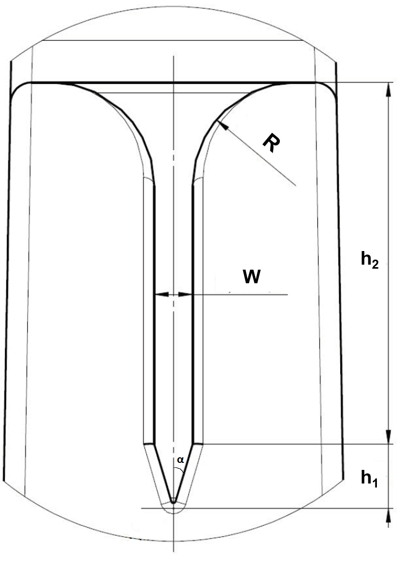
V 홈 치수
그림 1. V 홈 채널의 단면 치수 : W = 150 μm, h1 = 300 μm, h2 = 1200 μm, α = 14.5ο.

University at Buffalo와 University of Grenoble의 연구원들의 최근 논문에서 마이크로 그루브가 잠재적으로 모세관 효과를 향상시킬 수있는 방법을 보여주었습니다 [1]. 이 논문의 결과를 바탕으로, FLOW-3D를 사용하여 평행 한 플레이트로 대체 된 좁은 V- 홈 마이크로 채널 내부 유체의 자발적 모세관 흐름 (SCF)에 대한 사례 연구를 논의 할 것  입니다. 모세관 흐름의 시작에 대한 특정 조건이 충족되면 혈류를 모니터링하기위한 POC 시스템의 설계를 위해 전혈과 같은 점성 유체를 사용해도 큰 유체 속도를 얻을 수 있습니다.

모세관 흐름의 조건은 Gibbs 자유 에너지의 최소화를 기반으로 한 정적 접근 방식을 사용하여 이론적으로 설정할 수 있습니다. 보다 구체적으로, 입구 압력이 0 일 때 모세관 흐름이 시작되는 조건은 다음과 같습니다.

(수식 1)           pF/pW < cos⁡ θ

여기서  θ  는 영 접촉각이고  F  및  W  는 각각 유동의 임의 단면에서 자유 및 습식 둘레입니다. 그림 1에 표시된 것과 같은 반각 α 를 갖는 V- 홈 마이크로 채널의  경우 몇 가지 수학적 조작 후 eq. 1은 다음과 같이 다시 작성할 수 있습니다.

(수식 2)         sin α = cos⁡ θ

우리의 경우  α  ≈ 14.5 ο 가 있으므로 모세관 흐름의 조건은  θ  <75.5 o 입니다.

FLOW-3D 에서 시뮬레이션

정적 접근 방식이 SCF의 시작에 관한 중요한 정보를 제공하지만 수치 접근 방식은 현장 진료 장치에서 유동 역학을 연구하는 데 더 적합합니다. 접촉각이 37 °  이고 전혈의 유체 특성 을 갖는 V- 홈 마이크로 채널에 대해 CFD 분석을 수행했습니다 . 혈액의 점도는 거의 일정하기 때문에 흐름 체제는 뉴턴으로 간주됩니다 [1]. 유체 운동이 모세관 효과에 의해서만 발생하도록 모든 경계와 계산 영역 전체에 균일 한 주변 압력이 적용되었습니다. 시뮬레이션은 처음 4mm의 유체 이동을 포함하는 초기 시뮬레이션과 4mm에서 8mm의 유체 이동을 예측하는 재시작 시뮬레이션의 두 부분으로 나뉩니다.

결과 및 검증

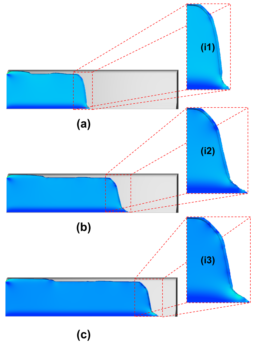
처음 8mm 이동에 대한 유동 역학은 그림 2에 나와 있습니다.이 그림은 세 가지 다른 시간에 슬롯에서 전진 인터페이스의 모양을 보여줍니다. 필라멘트 (Concus-Finn 필라멘트)의 점진적인 확장은 주 흐름보다 앞서 볼 수 있습니다.

모세관 흐름 시뮬레이션
그림 2. 세 가지 다른 시간에서 FLOW-3D를 사용하여 진행하는 모세관 흐름의 동적 계산 : (a) 0.04, (b) 0.07 및 (c) 0.11 초와 삽입물 (i1), (i2) 및 (i3) Concus-Finn 필라멘트의 진화 [1].

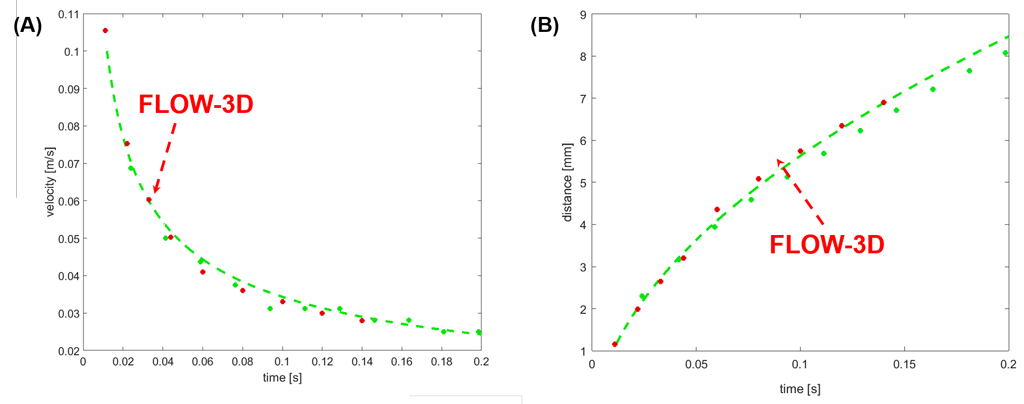
분석, 수치 및 실험 결과 간의 비교는 그림 3에 나와 있습니다. 수치 예측과 실험 간에는 탁월한 일치가 있습니다. 분석 솔루션도 플롯되었지만 채널 하단에있는 Concus – Finn 필라멘트의 효과가 고려되지 않았기 때문에 수치 및 실험 결과에 대한 유효한 비교를 나타내지 않을 수 있습니다.

모세관 흐름 검증
그림 3. (A) 시간의 함수로서 채널의 속도. 빨간색 점 : FLOW-3D 시뮬레이션 (중간 높이에서); 녹색 점 : 실험 관찰 (채널 중앙 높이); 파선 녹색 선 : 하단 V 홈의 효과를 무시한 분석 속도. (B) 시간의 함수로서 액체 전면의 원점으로부터의 거리. 빨간색 점 : FLOW-3D 시뮬레이션 (중간 높이에서); 녹색 점 : 실험 관찰 (채널 중앙 높이); 파선 녹색 선 : 하단 V 홈의 효과를 무시한 분석 속도 [1].

전혈 이외에도 식용 색소로 착색 한 물과 점성이 높은 알기 네이트 용액을 포함하여 장치가 고점도 유체를 이동시킬 수있는 가능성을 테스트하는 등 다양한 유체를 연구했습니다. 혈액과 같은 고점도 액체는 1 초 이내에 이동할 수 있습니다 (아래 애니메이션 참조).https://www.youtube.com/embed/v4OYoHStJ1w?controls=1&rel=0&playsinline=0&modestbranding=0&autoplay=0&enablejsapi=1&origin=https%3A%2F%2Fwww.flow3d.com&widgetid=1

사례 연구는 상대적으로 큰 점도 (물의 4 배)를 갖는 전혈의 경우 최대 7.5cm / s의 속도를 달성했음을 보여줍니다. 실험 결과 및  FLOW-3D  예측에 따라 전체 채널은 0.2 초 이내에 혈액으로 채워졌습니다. FLOW-3D  시뮬레이션 결과는 실험 관찰 결과와 매우 일치하며, V-groove 내부의 거리에 따라 속도가 감소하지만 장치의 전체 길이에 걸쳐 중요 함을 나타냅니다.

참고 문헌

  1. Berthier, J., K. Brakke, E. P. Furlani, I. H. Karampelas, and G. Delapierre. “Open-surface microfluidics.” In Proceedings of the Nanotech International Conference, pp. 15-19. 2014.
  2. Hirt, Cyril W., and Billy D. Nichols. “Volume of fluid (VOF) method for the dynamics of free boundaries.” Journal of computational physics 39, no. 1 (1981): 201-225.
  3. Rajaratnam, N., and M. R. Chamani. “Energy loss at drops.” Journal of Hydraulic Research 33, no. 3 (1995): 373-384.
The Simulation of Droplet Impact on the Super-Hydrophobic Surface with Micro-Pillar Arrays Fabricated by Laser Irradiation and Silanization Processes

The simulation of droplet impact on the super-hydrophobic surface with micro-pillar arrays fabricated by laser irradiation and silanization processes

레이저 조사 및 silanization 공정으로 제작된 micro-pillar arrays를 사용하여 초 소수성 표면에 대한 액적 영향 시뮬레이션

ZhenyanXiaa YangZhaoa ZhenYangabc ChengjuanYangab LinanLia ShibinWanga MengWangab
aSchool of Mechanical Engineering, Tianjin University, Tianjin, 300054, China
bKey Laboratory of Mechanism Theory and Equipment Design of Ministry of Education, Tianjin, 300072, Chinac
School of Engineering, University of Warwick, Coventry, CV4 7AL, UK

Received 23 September 2020, Revised 17 November 2020, Accepted 26 November 2020, Available online 11 December 2020.

Abstract

Super-hydrophobicity is one of the significant natural phenomena, which has inspired researchers to fabricate artificial smart materials using advanced manufacturing techniques. In this study, a super-hydrophobic aluminum surface was prepared by nanosecond laser texturing and FAS modification in sequence. The surface wettability turned from original hydrophilicity to super-hydrophilicity immediately after laser treatment. Then it changed to super-hydrophobicity showing a WCA of 157.6 ± 1.2° with a SA of 1.7 ± 0.7° when the laser-induced rough surface being coated with a layer of FAS molecules. The transforming mechanism was further explored from physical and chemical aspects based on the analyses of surface morphology and surface chemistry. Besides, the motion process of droplet impacting super-hydrophobic surface was systematically analyzed via the optimization of simulation calculation grid and the simulation method of volume of fluid (VOF). Based on this simulation method, the morphological changes, the inside pressure distribution and velocity of the droplet were further investigated. And the motion mechanism of the droplet on super-hydrophobic surface was clearly revealed in this paper. The simulation results and the images captured by high-speed camera were highly consistent, which indicated that the computational fluid dynamics (CFD) is an effective method to predict the droplet motion on super- hydrophobic surfaces. This paper can provide an explicit guidance for the selection of suitable methods for functional surfaces with different requirements in the industry.

Korea Abstract

초 소수성은 연구원들이 첨단 제조 기술을 사용하여 인공 스마트 재료를 제작하도록 영감을 준 중요한 자연 현상 중 하나 입니다. 이 연구에서 초 소수성 알루미늄 표면은 나노초 레이저 텍스처링과 FAS 수정에 의해 순서대로 준비되었습니다.

레이저 처리 직후 표면 습윤성은 원래의 친수성에서 초 친수성으로 바뀌 었습니다. 그런 다음 레이저 유도 거친 표면을 FAS 분자 층으로 코팅했을 때 WCA가 157.6 ± 1.2 °이고 SA가 1.7 ± 0.7 ° 인 초 소수성으로 변경되었습니다.

변형 메커니즘은 표면 형태 및 표면 화학 분석을 기반으로 물리적 및 화학적 측면에서 추가로 탐구 되었습니다. 또한, 초 소수성 표면에 영향을 미치는 물방울의 운동 과정은 시뮬레이션 계산 그리드의 최적화와 유체 부피 (VOF) 시뮬레이션 방법을 통해 체계적으로 분석되었습니다.

이 시뮬레이션 방법을 바탕으로 형태학적 변화, 내부 압력 분포 및 액 적의 속도를 추가로 조사했습니다. 그리고 초 소수성 표면에 있는 물방울의 운동 메커니즘이 이 논문에서 분명하게 드러났습니다.

시뮬레이션 결과와 고속 카메라로 캡처한 이미지는 매우 일관적 이었습니다. 이는 전산 유체 역학 (CFD)이 초 소수성 표면에서 액적 움직임을 예측하는 효과적인 방법임을 나타냅니다.

이 백서는 업계의 다양한 요구 사항을 가진 기능 표면에 적합한 방법을 선택하기 위한 명시적인 지침을 제공 할 수 있습니다.

Keywords: Laser irradiation; Wettability; Droplet impact; Simulation; VOF

Introduction

서식지에 적응하기 위해 많은 자연 식물과 동물에서 특별한 습윤 표면이 진화되었습니다 [1-3]. 연잎은 먼지에 의한 오염으로부터 스스로를 보호하기 위해 우수한 자가 청소 특성을 나타냅니다 [4]. 사막 딱정벌레는 공기에서 물을 수확할 수 있는 기능적 표면 때문에 건조한 사막에서 생존 할 수 있습니다 [5].

자연 세계에서 영감을 받아 고체 기질의 표면 습윤성을 수정하는데 더 많은 관심이 집중되었습니다 [6-7]. 기능성 표면의 우수한 성능은 고유 한 표면 습윤성에 기인하며, 이는 고체 표면에서 액체의 확산 능력을 반영하는 중요한 특성 중 하나입니다 [8].

일반적으로 물 접촉각 (WCA) 값에 따라 90 °는 친수성과 소수성의 경계로 간주됩니다. WCA가 90 ° 이상인 소수성 표면, WCA가 90 ° 미만인 친수성 표면 [9 ]. 특히 고체 표면은 WCA가 10 ° 미만의 슬라이딩 각도 (SA)에서 150 °를 초과 할 때 특별한 초 소수성을 나타냅니다 [10-11].

<내용 중략> ……

 The Simulation of Droplet Impact on the Super-Hydrophobic Surface with Micro-Pillar Arrays Fabricated by Laser Irradiation and Silanization Processes
The Simulation of Droplet Impact on the Super-Hydrophobic Surface with Micro-Pillar Arrays Fabricated by Laser Irradiation and Silanization Processes

References

[1] H.W. Chen, P.F. Zhang, L.W. Zhang, Y. Jiang, H.L. Liu, D.Y. Zhang, Z.W. Han, L.
Jiang, Continuous directional water transport on the peristome surface of Nepenthes
alata, Nature 532 (2016) 85-89.
[2] Y. Liu, K.T. Zhang, W.G. Yao, J.A. Liu, Z.W. Han, L.Q. Ren, Bioinspired
structured superhydrophobic and superoleophilic stainless steel mesh for efficient oilwater separation, Colloids Surf., A 500 (2016) 54-63.
[3] Y.X. Liu, W.L. Liu, G.L. Wang, J.C. Hou, H. Kong, W.L. Wang, A facile one-step
approach to superhydrophilic silica film with hierarchical structure using
fluoroalkylsilane, Colloids Surf., A 539 (2018) 109-115.
[4] F.P. Wang, S. Li, L. Wang, Fabrication of artificial super-hydrophobic lotus-leaflike bamboo surfaces through soft lithography, Colloids Surf., A 513 (2017) 389-395.
[5] W. Huang, X.Y. Tang, Z. Qiu, W.X. Zhu, Y.G. Wang, Y.L. Zhu, Z.F. Xiao, H.G.
Wang, D.X. Liang, Jian, L. Y.J Xie, Cellulose-based Superhydrophobic Surface
Decorated with Functional Groups Showing Distinct Wetting Abilities to Manipulate
Water Harvesting, ACS Appl. Mater. Interfaces DOI: 10.1021/acsami.0c12504.
[6] M.Y. Zhang, L.J. Ma, Q. Wang, P. Hao, X. Zheng, Wettability behavior of
nanodroplets on copper surfaces with hierarchical nanostructures, Colloids Surf., A
604 (2020) 125291.
[7] A.F. Pan, W.J. Wang, X.S. Mei, K.D. Wang, X.B. Yang, Rutile TiO2 flocculent
ripples with high antireflectivity and superhydrophobicity on the surface of titanium
under 10 ns laser irradiation without focusing, Langmuir 33 (2017) 9530-9538.
[8] M. Li, X.H. Liu, N. Liu, Z.H. Guo, P.K. Singh, S.Y. Fu, Effect of surface
wettability on the antibacterial activity of nanocellulose-based material with
quaternary ammonium groups, Colloids Surf., A 554 (2018) 122-128.
[9] T.C. Chen, H.T. Liu, H.F. Yang, W. Yan, W. Zhu, H. Liu, Biomimetic fabrication
of robust self-assembly superhydrophobic surfaces with corrosion resistance
properties on stainless steel substrate, RSC Adv. 6 (2016) 43937-43949.
[10] P. Zhang, F.Y. Lv, A review of the recent advances in superhydrophobic surfaces
and the emerging energy-related applications, Energy 82 (2015) 1068-1087.
[11] Z. Yang, X.P. Liu, Y.L. Tian, Novel metal-organic super-hydrophobic surface
fabricated by nanosecond laser irradiation in solution, Colloids Surf., A 587 (2020)
124343.
[12] J.Y. Peng, X.J. Zhao, W.F. Wang, X. Gong, Durable Self-Cleaning Surfaces with
Superhydrophobic and Highly Oleophobic Properties, Langmuir, 35 (2019) 8404-
8412.
[13] Z. Yang, X.P. Liu, Y.L. Tian, A contrastive investigation on anticorrosive
performance of laser-induced super-hydrophobic and oil-infused slippery coatings,
Prog. Org. Coat. 138 (2020) 105313.
[14] J.L. Yong, F. Chen, Q. Yang, J.L. Huo, X. Hou, Superoleophobic Surfaces,
Chem. Soc. Rev. 46 (2017) 4168-4217.
[15] D.W. Li, H.Y. Wang, Y. Liu, D.S. Wei, Z.X. Zhao, Large-Scale Fabrication of
Durable and Robust Super-Hydrophobic Spray Coatings with Excellent Repairable
and Anti-Corrosion Performance, Chem. Eng. J. 367 (2019) 169-179.
[16] R.J. Liao, Z.P. Zuo, C. Guo, Y. Yuan, A.Y. Zhuang, Fabrication of
superhydrophobic surface on aluminum by continuous chemical etching and its antiicing property, Appl. Surf. Sci. 317 (2014) 701-709.
[17] Z. Yang. X.P. Liu, Y.L. Tian, Hybrid laser ablation and chemical modification for
fast fabrication of bio-inspired super-hydrophobic surface with excellent selfcleaning, stability and corrosion resistance, J Bionic Eng 16 (2019) 13-26.
[18] Z. Yang, Y.L. Tian, Y.C. Zhao, C.J. Yang, Study on the fabrication of superhydrophobic surface on Inconel alloy via nanosecond laser ablation, Materials 12
(2019) 278.
[19] Y. Wang, X. Gong, Superhydrophobic Coatings with Periodic Ring Structured
Patterns for Self-Cleaning and Oil-Water Separation, Adv. Mater. Interfaces 4 (2017)
1700190.
[20] N. Chik, W.S.W.M. Zain, A.J. Mohamad, M.Z. Sidek, W.H.W. Ibrahim, A. Reif,
J.H. Rakebrandt, W. Pfleging, X. Liu, Bacterial adhesion on the titanium and
stainless-steel surfaces undergone two different treatment methods: Polishing and ultrafast laser treatment, IOP Conf. Ser.: Mater. Sci. Eng.358 (2018) 012034.
[21] N.K.K. Win, P. Jitareerat, S. Kanlayanarat, S. Sangchote, Effects of cinnamon
extract, chitosan coating, hot water treatment and their combinations on crown rot
disease and quality of banana fruit, Postharvest Biol. Technol. 45 (2007) 333–340.
[22] A. Yarin, Drop impact dynamics: splashing, spreading, receding, bouncing, Annu.
Rev. Fluid Mech. 38 (2006) 159–192.
[23] N. Wang, L.L. Tang, Y.F. Cai, W. Tong, D.S. Xiong, Scalable superhydrophobic
coating with controllable wettability and investigations of its drag reduction, Colloids
Surf. A 555 (2018) 290–295.
[24] R. Fürstner, W. Barthlott, C. Neinhuis, P. Walzel, Wetting and self-cleaning
properties of artificial superhydrophobic surfaces, Langmuir 21 (2005) 956–61.
[25] U. Trdan, M. Hočevar, P. Gregorčič, Transition from superhydrophilic to
superhydrophobic state of laser textured stainless steel surface and its effect on
corrosion resistance, Corros. Sci. 123 (2017) 21–44.
[26] A.L. Biance, C. Clanet, D. Quere, First steps in the spreading of a liquid droplet,
Phys. Rev. E 69 (2004) 016301.
[27] S. Kulju, L. Riegger, P. Koltay et al, Fluid flow simulations meet high-speed
video: computer vision comparison of droplet dynamics, J. Colloid Interface Sci. 522
(2018) 48.
[28] C.J. Yong, B. Bhushan, Dynamic effects of bouncing water droplets on
superhydrophobic surfaces, Langmuir 24.12 (2008) 6262–6269.
[29] G. Karapetsas, N.T. Chamakos, A.G. Papathanasiou, Efficient modelling of
droplet dynamics on complex surfaces, J. Phys.: Condens. Matter 28.8 (2016) 085101.
[30] D. Khojasteh, N.M. Kazerooni, S. Salarian et al, Droplet impact on
superhydrophobic surfaces: a review of recent developments, J. Ind. Eng. Chem. 42
(2016) 1–14.
[31] S.H. Kim, Y. Jiang, H. Kim, Droplet impact and LFP on wettability and
nanostructured surface, Exp. Therm. Fluid Sci. 99 (2018) 85–93.
[32] M. Rudman, Volume‐Tracking Methods for Interfacial Flow Calculations, Int.
J. Numer. Methods Fluids 24.7 (1997) 671-691.

A new dynamic masking technique for time resolved PIV analysis

A new dynamic masking technique for time resolved PIV analysis

시간 분해 PIV 분석을위한 새로운 동적 마스킹 기술

물체 가시성을 허용하기 위해 형광 코팅과 결합 된 새로운 프리웨어 레이 캐스팅 도구

Journal of Visualization ( 2021 ) 이 기사 인용

Abstract

Time resolved PIV encompassing moving and/or deformable objects interfering with the light source requires the employment of dynamic masking (DM). A few DM techniques have been recently developed, mainly in microfluidics and multiphase flows fields. Most of them require ad-hoc design of the experimental setup, and may spoil the accuracy of the resulting PIV analysis. A new DM technique is here presented which envisages, along with a dedicated masking algorithm, the employment of fluorescent coating to allow for accurate tracking of the object. We show results from measurements obtained through a validated PIV setup demonstrating the need to include a DM step even for objects featuring limited displacements. We compare the proposed algorithm with both a no-masking and a static masking solution. In the framework of developing low cost, flexible and accurate PIV setups, the proposed algorithm is made available through a freeware application able to generate masks to be used by an existing, freeware PIV analysis package.

광원을 방해하는 이동 또는 변형 가능한 물체를 포함하는 시간 해결 PIV는 동적 마스킹 (DM)을 사용해야 합니다. 주로 미세 유체 및 다상 흐름 분야에서 몇 가지 DM 기술이 최근 개발되었습니다. 대부분은 실험 설정의 임시 설계가 필요하며 결과 PIV 분석의 정확도를 떨어 뜨릴 수 있습니다. 여기에는 전용 마스킹 알고리즘과 함께 형광 코팅을 사용하여 물체를 정확하게 추적 할 수있는 새로운 DM 기술이 제시되어 있습니다. 제한된 변위를 특징으로 하는 물체에 대해서도 DM 단계를 포함해야 하는 필요성을 보여주는 검증 된 PIV 설정을 통해 얻은 측정 결과를 보여줍니다. 제안 된 알고리즘을 no-masking 및 static masking 솔루션과 비교합니다. 저비용, 유연하고 정확한 PIV 설정 개발 프레임 워크에서 제안 된 알고리즘은 기존 프리웨어 PIV 분석 패키지에서 사용할 마스크를 생성 할 수 있는 프리웨어 애플리케이션을 통해 사용할 수 있습니다.

Keywords

  • Time resolved PIV, Dynamics masking, Image processing, Vibration inducers, Fluorescent coating

그래픽 개요

소개

PIV (입자 영상 속도계)의 사용은 70 년대 후반 (Archbold 및 Ennos 1972 )이 반점 계측의 확장 (Barker and Fourney 1977 ) 으로 도입된 이래 실험 유체 역학에서 중심적인 역할을 했습니다 . PIV 기술의 기본 아이디어는 유체에 주입된 입자의 속도를 측정하여 유동장을 재구성하는 것입니다. 입자의 크기와 밀도는 확실하게 선택되고 유동을 만족스럽게 따르게 됩니다.

흐름은 레이저 / LED 소스를 통해 조명되고 입자에 의해 산란 된 빛은 추적을 허용합니다. 독자는 리뷰 작품 Grant ( 1997 ), Westerweel et al. ( 2013 년)에 대한 자세한 설명을 참조하십시오. 기본 2D 기술은 고유한 설정으로 발전했으며, 가장 진보 된 것은 단일 / 다중 평면 입체 PIV (Prasad 2000 ) 및 체적 / 단층 PIV (Scarano 2013 )입니다. 광범위한 유동장의 비 침습적 측정이 필요한 산업 및 연구 응용 분야에서 광범위하게 사용되었습니다.

조사된 유동장이 단단한 서있는 경계의 영향을 받는 경우 정적 마스킹 (SM) 접근 방식을 사용하여 PIV 분석을 수행하는 영역에서 솔리드 객체와 그림자가 차지하는 영역을 빼기 위해 주의를 기울여야 합니다. 실제로 이러한 영역에서는 파종 입자를 식별 할 수 없으므로 유속 재구성을 수행 할 수 없습니다. 제대로 처리되지 않으면 이 마스킹 단계는 잘못된 예측으로 이어질 수 있으며, 불행히도 그림자 영역 경계의 근접성에 국한되지 않습니다.

PIV 기술은 획득 프레임 속도를 관심있는 시간 척도로 조정하여 정상 상태 또는 시간 변화 흐름에 적용 할 수 있습니다. 시간의 가변성이 고체 물체의 위치 / 모양과 관련된 경우 이미지를 동적으로 마스킹하기 위해 추가 노력이 필요합니다. 고체 물체뿐만 아니라 다른 유체 단계도 가려야한다는 점에 유의해야합니다 (Foeth et al. 2006). 

이 프로세스는 고체 물체의 움직임이 선험적으로 알려진 경우 비교적 쉬우므로 SM 알고리즘에 대한 최소한의 수정이 목적에 부합 할 수 있습니다. 그러나 고체 물체의 위치 및 / 또는 모양이 알려지지 않은 방식으로 시간에 따라 변할 경우 물체를 동적으로 추적 할 수 있는 마스킹 기술이 필요합니다. PIV 분석을위한 동적 마스킹 (DM) 접근 방식은 현재 상당한 주목을 받고 있습니다 (Sanchis and Jensen 2011 , Masullo 및 Theunissen 2017 , Anders et al. 2019 ) . 시간 분해 PIV 시스템의 확산 덕분에 고속 카메라의 가용성이 높아집니다. 

DM 기술의 주요 발전은 마이크로 PIV 분야에서 비롯됩니다 (Lindken et al. 2009) 마이크로 및 나노 스위 머 (Ergin et al. 2015 ) 및 다상 흐름 (Brücker 2000 , Khalitov 및 Longmire 2002 ) 주변의 유동장을 조사 하려면 정확하고 유연한 알고리즘이 필요합니다. DM 기술은 상용 PIV 분석 소프트웨어 패키지 (TSI Instruments 2014 , DantecDynamics 2018 )에 포함되어 있습니다. 최근 개발 (Vennemann 및 Rösgen 2020 )은 신경망 자동 마스킹 기술의 적용을 예상하지만, 네트워크를 훈련하려면 합성 데이터 세트를 생성해야합니다.

많은 알고리즘은 이미지 처리 기술을 사용하여 개체를 추적하며, 대부분 사용자는 획득 한 이미지에서 추적 할 개체를 강조 표시 할 수있는 임시 실험 설정을 개발해야합니다. 따라서 실험 설정의 설계는 알고리즘의 최종 정확도에 영향을줍니다.

몇 가지 해결책을 구상 할 수 있습니다. 다음에서는 간단한 2D PIV 설정을 참조하지만 대부분의 고려 사항은 더 복잡한 설정으로 확장 할 수 있습니다. PIV 설정에서 객체를 쉽고 정확하게 추적 할 수 있도록 렌더링하는 가장 간단한 방법은 일반적으로 PIV 레이저 시트에 대략 수직 인 카메라를 향한 반사를 최대화하는 방향을 가리키는 추가 광원을 사용하여 조명하는 것입니다. 이 순진한 솔루션과 관련된 주요 문제는 PIV의 ROI (관심 영역)를 비추 지 않고는 광원을 움직이는 물체에만 겨냥하는 것이 사실상 불가능하여 시딩에 의해 산란 된 레이저 광 사이의 명암비를 감소 시킨다는 것입니다. 입자와 어두운 배경.

카메라의 프레임 속도가 높을수록 센서에 닿는 빛의 양이 적다는 사실로 인해 상황이 가혹 해집니다. 고체 물체의 움직임과 유동 입자가 모두 사용 된 설정의 획득 속도에 비해 충분히 느리다면, 가능한 해결책은 레이저 펄스 쌍 사이에 단일 확산 광 샷을 삽입하는 것입니다 (반드시 대칭 삽입은 아님). 그리고 카메라 샷을 둘 모두에 동기화합니다. 각 레이저 커플에서 물체의 위치는 확산 광에 의해 생성 된 이전 샷과 다음 샷의 두 위치를 보간하여 결정될 수 있습니다. 이 접근 방식에는 레이저, 카메라 및 빛을 제어 할 수있는 동기화 장치가 필요합니다.

이 문제에 대한 해결책이 제안되었으며 유체 인터페이스 (Foeth et al. 2006 ; Dussol et al. 2016 ) 의 밝은 반사를 활용 하여 이미지에서 많은 양의 산란 레이저 광을 획득 할 수 있습니다. 고체 표면에는 효과를 높이기 위해 반사 코팅이 제공 될 수 있습니다. 그런 다음 물체는 비정상적으로 큰 입자로 식별되고 경계를 쉽게 추적 할 수 있습니다. 이 솔루션의 단점은 물체 표면에서 산란 된 빛이 레이저 시트에 있지 않은 많은 시딩 입자를 비추어 PIV 분석의 정확도를 점진적으로 저하 시킨다는 것입니다.

위의 접근 방식의 개선은 다른 파장 의 두 번째 동일 평면 레이저 시트 (Driscoll et al. 2003 )를 사용합니다. 첫 번째 레이저 파장을 중심으로 한 좁은 반사 대역. 전체 설정은 매우 비쌀 수 있습니다. 파장 방출의 차이를 이용하여 설정을 저렴하게 만들 수 있습니다. 서로 다른 필터가 장착 된 두 대의 카메라를 적용하면 인터페이스로부터의 반사와 독립적으로 형광 시드 입자를 식별 할 수 있습니다 (Pedocchi et al. 2008 ).

객체의 변위가 작을 때 기본 솔루션은 실제 시간에 따라 변하는 음영 영역에 가장 근접한 하나의 정적 마스크를 추출하는 것입니다. 일반적인 경험 법칙은 예상되는 음영 영역보다 약간 더 크게 마스크를 그려 분석에 포함 된 조명 영역의 양을 단순화하고 최소화하는 것 사이의 최상의 균형을 찾는 것입니다.

본 논문에서는 PIV 분석을위한 DM 문제에 대한 새로운 실험적 접근법을 제안합니다. 우리의 방법은 형광 페인팅을 사용하여 물체를 쉽게 추적 할 수 있도록 하는 기술과 시변 마스크를 생성 할 수있는 특정 오픈 소스 알고리즘을 포함합니다. 이 접근법은 레이저 광에 불투명 한 물체의 큰 변위를 허용함으로써 효과적인 것으로 입증되었습니다. 

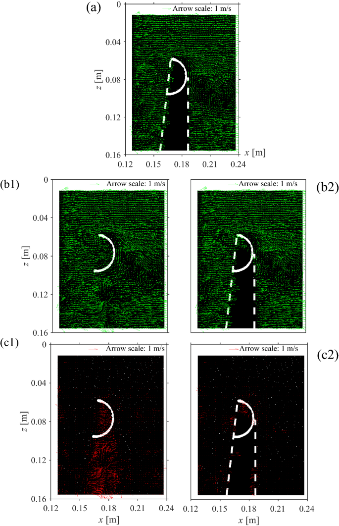
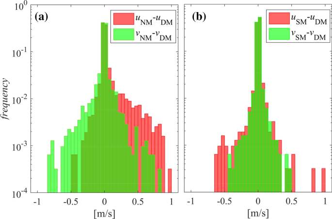
우리의 방법인 NM (no-masking)과 SM (static masking) 접근 방식을 비교합니다. 우리의 접근 방식의 타당성을 입증하는 것 외에도 이 백서는 마스킹 단계가 정확한 결과를 얻기 위해 가장 중요하다는 것을 확인합니다. 실제로 물체의 변위가 무시할 수 없는 경우 DM에 대한 리조트는 필수이며 SM 접근 방식은 음영 처리 된 영역의 주변 환경에 국한되지 않는 부정확성을 유발합니다. 

논문의 구조는 다음과 같습니다. 먼저 형광 코팅 기술과 마스킹 소프트웨어를 설명하는 제안된 접근법의 근거를 소개합니다. 그런 다음 PIV 설정에 대한 설명 후 두 벤치 마크 사례를 통해 전체 PIV 체인 분석의 신뢰성을 평가합니다. 그런 다음 제안 된 DM 방법의 결과를 NM 및 SM 솔루션과 비교합니다. 마지막으로 몇 가지 결론이 도출됩니다.

행동 양식

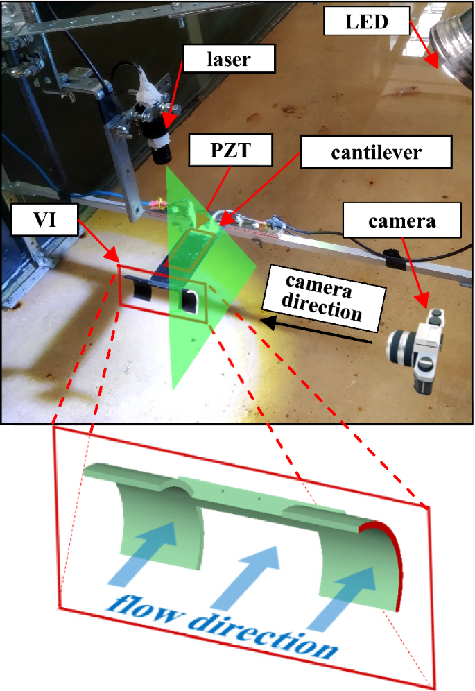
제안 된 DM 기술은 PIV 분석을 위해 캡처 한 동일한 이미지에서 쉽고 정확한 추적 성을 허용하기 위해 움직이는 물체 표면의 형광 코팅을 구상합니다. 물체가 가시화되면 특정 알고리즘이 물체 추적을 수행하고 레이저 위치가 알려지면 (그림 1 참조  ) 음영 영역의 마스킹을 수행합니다.

형광 코팅

코팅은 구조적 매트릭스 에 시판되는 형광 분말 (fluorescein (Taniguchi and Lindsey 2018 ; Taniguchi et al. 2018 )) 의 분산액으로 구성됩니다 . 단단한 물체의 경우 매트릭스는 폴리 에스터 / 에폭시 (대상 재료와의 화학적 호환성에 따라) 투명 수지 일 수 있습니다. 변형 가능한 물체의 경우 매트릭스는 투명한 실리콘 고무로 만들 수 있습니다. 형광 코팅 된 물체는 실행 중에 지속적으로 빛을 방출하기 위해 실험 전에 충분히 오랫동안 조명을 비춰 야합니다. 우리는 4W LED 소스 (그림 2 에서 볼 수 있음)에 20 초 긴 노출이  실험 실행 (몇 초)의 짧은 기간 동안 일관된 형광 방출을 제공하기에 충분하다는 것을 발견했습니다.

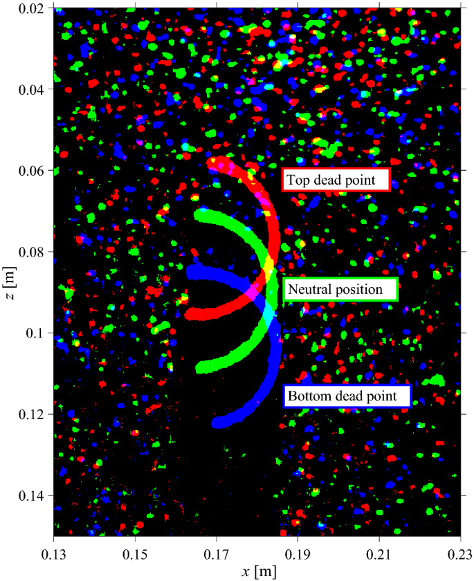
우리 실험에서 물체와 입자 크기 사이의 상당한 차이를 감안할 때 전자를 식별하는 것은 간단합니다. 그림  3 은 씨 뿌리기 입자와 물체 모양이 서로 다른 세 번에 겹쳐진 모습을 보여줍니다 (색상은 다른 순간을 나타냄).

대신, 이러한 크기 기반 분류가 가능하지 않은 경우 입자와 물체의 파장을 분리해야합니다. 이러한 분리는 시드 입자에 의해 산란 된 빛과 현저하게 다른 파장에서 방출되는 형광 코팅을 선택하여 달성 할 수 있습니다. 또는 레이저에서 멀리 떨어진 대역에서 방출되는 형광 입자를 이용하는 것 (Pedocchi et al. 2008 ). 두 경우 모두 컬러 이미지 획득의 채널 분리 또는 멀티 카메라 설정의 애드혹 필터링은 물체 식별을 크게 촉진 할 수 있습니다. 우리의 경우에는 그러한 파장 분리를 달성 할 필요가 없습니다. 실제로 형광 코팅의 방출 스펙트럼의 피크는 540nm입니다 (Taniguchi and Lindsey 2018 ; Taniguchi et al. 2018), 사용 된 레이저의 532 nm에 매우 가깝습니다.

마스킹 소프트웨어

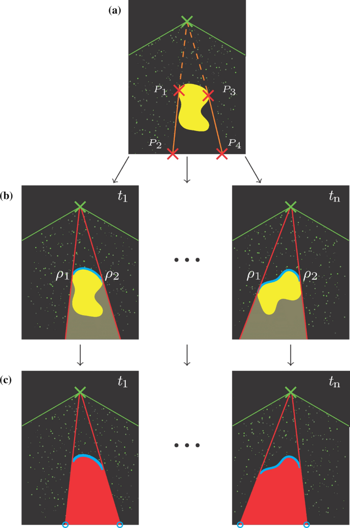
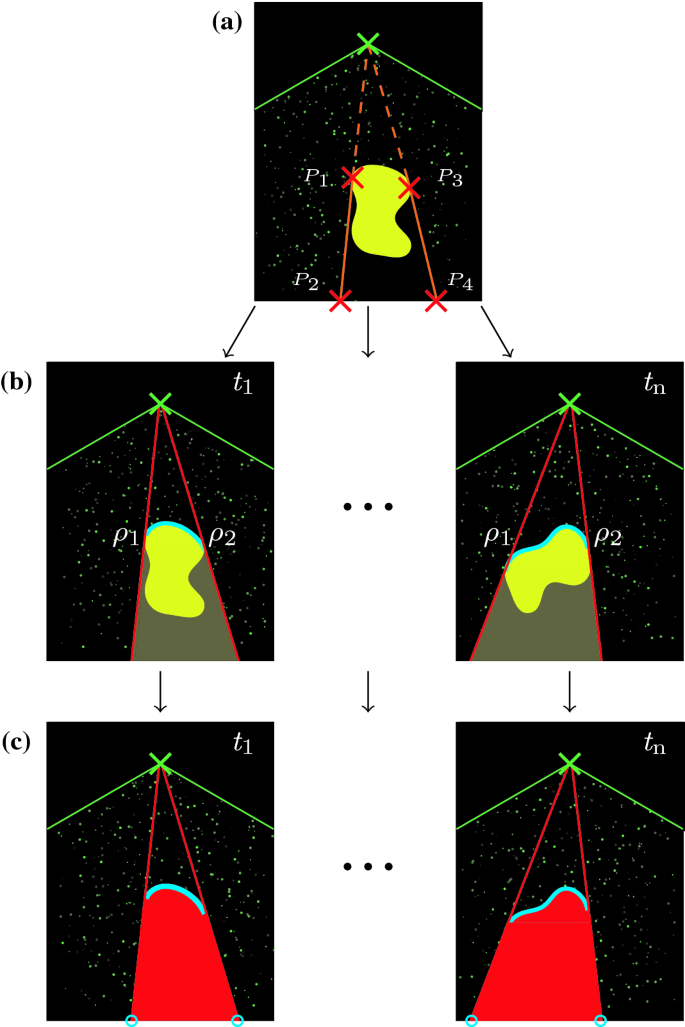
DM 용으로 개발 된 알고리즘 은 무료 PIV 분석 패키지 PIVlab (Thielicke 2020 , Thielicke 및 Stamhuis 2014 ) 과 함께 작동하도록 고안된 오픈 소스 프리웨어 GUI 기반 도구 (Prestininzi 및 Lombardi 2021 )입니다. 이것은 세 단계의 순차적 실행으로 구성됩니다 (그림 1 에서 a–b–c라고 함 ). 첫 번째 단계 (a)는 장면에서 레이저 위치를 찾는 데 사용됩니다 (즉, 소스의 좌표를 계산합니다. 장애물에 부딪히는 빛); 두 번째 항목 (b)은 개체 위치를 추적하고 각 프레임의 음영 영역을 계산합니다. 세 번째 항목 (c)은 추적 된 개체 영역과 음영 처리 된 개체 영역을 PIV 알고리즘을위한 단일 마스크로 병합합니다.

각 단계에 대한 자세한 내용은 다음과 같습니다.

  1. (ㅏ)레이저 위치는 프레임 (즉, 획득 한 프레임의 시야 (FOV)) 내에서 가시적 일 수도 있고 아닐 수도 있습니다. 전자의 경우 사용자는 GUI에서 레이저 소스를 클릭하여 찾기 만하면됩니다. 후자의 경우, 사용자는 음영 영역의 경계에 속하는 두 개의 세그먼트 (두 쌍의 점)를 그리도록 요청받습니다. 그러면 FOV 외부에있는 레이저 위치가 두 선의 교차점으로 계산됩니다. 세그먼트로 구성됩니다. 개체 그림자는 ROI 프레임 상자에 도달하는 것으로 간주됩니다.
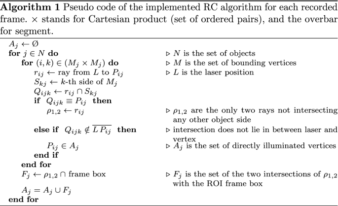
  2. (비)레이저 위치가 알려지면 물체 추적은 다음과 같이 수행됩니다. 각 프레임의 하나의 채널 (이 경우 RGB 색상 공간이 사용되기 때문에 녹색 채널이지만 GUI는 선호하는 채널을 지정할 수 있음)은 다음과 같습니다. 로컬 적응 임계 값을 사용하여 이진화 됨 (Bradley and Roth 2007), 후자는 이웃 주변의 로컬 평균 강도를 사용하여 각 픽셀에 대해 계산됩니다. 그런 다음 입자와 물체로 구성된 이진 이미지가 영역으로 변환됩니다. 우리 실험에 존재하는 유일한 장애물은 모든 입자에 비해 더 큰 크기를 기준으로 식별됩니다. 다른 전략은 이전에 논의되었습니다. 그런 다음 장애물 영역의 경계 다각형은 사용자 정의 포인트 밀도로 결정됩니다. 여기에서는 그림자 결정을 위해 광선 투사 (RC) 접근 방식을 채택했습니다. RC는 컴퓨터 그래픽을 기반으로하는 “경 운송 모델링”의 틀에 속합니다. 수치 적으로 정확한 그림자를 제공하기 때문에 여기에서 선택됩니다. 정확도는 떨어지지 만 주로 RC의 계산 부하를 줄이는 것을 목표로하는 몇 가지 다른 방법이 개발되었습니다.2015 ), 여기서 간략히 회상합니다. 각 프레임 (명확성을 위해 여기에 색인화되지 않음)에 대해 광선아르 자형나는 j아르 자형나는제이레이저 위치 L 에서 i 번째 정점 으로 캐스트됩니다.피나는 j피나는제이의 J 오브젝트의 경계 다각형 일; 목표는피나는 j피나는제이 하위 집합에 속 ㅏ제이ㅏ제이 레이저에 의해 직접 조명되는 경계 정점의 피나는 j피나는제이 에 추가됩니다 ㅏ제이ㅏ제이 만약 아르 자형나는 j아르 자형나는제이 적어도 한쪽을 교차 에스k j에스케이제이( j 번째 개체 경계 다각형 의 모든면에 걸쳐있는 k )피나는 j피나는제이 (그것이 교차로 큐나는 j k큐나는제이케이 레이저 위치와 정점 사이에 있지 않습니다. 피나는 j피나는제이). 두 개의 광선, 즉ρ1ρ1 과 ρ2ρ2추가면을 가로 지르지 않는는 저장됩니다.
  3. (씨)일단 정점 세트, 즉 ㅏ제이ㅏ제이 레이저에 의해 직접 비춰지고 식별되었으며 ROI 프레임 상자의 음영 부분은 후자와 교차하여 결정됩니다. ρ1ρ1 과 ρ2ρ2. 두 교차점은 다음에 추가됩니다.ㅏ제이ㅏ제이. 점으로 둘러싸인 영역ㅏ제이ㅏ제이 마침내 마스크로 변환됩니다.

레이저 소스가 여러 개인 경우 각각에 RC 알고리즘을 적용해야하며 음영 영역의 결합이 수행됩니다. 레이 캐스팅 절차의 의사 코드는 Alg에보고됩니다. 1.

그림
그림 1
그림 1

DM 검증

이 섹션에서는 제안 된 DM으로 수행 된 PIV 측정과 두 가지 다른 접근 방식, 즉 no-masking (NM)과 static masking (SM) 간의 비교를 제시합니다.

그림 2
그림 2
그림 3
그림 3

실험 설정

진동 유도기 (VI)의 성능을 분석하기 위해 PIV 설정을 설계하고 현재 DM 기술을 개발했습니다 (Curatolo et al. 2019 , 2020 ). 후자는 비 맥동 ​​유체 흐름에서 역류에 배치 된 캔틸레버의 규칙적이고 넓은 진동을 유도 할 수있는 윙렛입니다. 이러한 VI는 캔틸레버의 끝에 장착되며 (그림 2 참조   ) 진동 운동의 어느 지점에서든 캔틸레버의 중립 구성을 향해 양력을 생성 할 수있는 두 개의 오목한 날개가 있습니다.

VI는 캔틸레버 표면에 장착 된 압전 패치를 사용하여 고정 유체 흐름에서 기계적 에너지 추출을 향상시킬 수 있습니다. 그림 2 에서 강조된 날개의 전체 측면 가장자리는  Sect에 설명 된 사양에 따라 형광 페인트로 코팅되어 있습니다. 2.1 . 실험은 Roma Tre University 공학부 수력 학 실험실의 자유 표면 채널에서 수행됩니다. 10.8cm 길이의 캔틸레버는 채널의 중심선에 배치되고 상류로 향하며 수직-세로 평면에서 진동합니다. 세라믹 페 로브 스카이 트 (PZT) 압전 패치 (7××캔틸레버의 윗면에는 Physik Instrumente (PI)에서 만든 3cm)가 부착되어 있습니다. 흐름 유도 진동 하에서 변형으로 인해 AC 전압 차이를 제공합니다. VI 왼쪽 날개의 수직 중앙면에있는 2D 속도 필드는 수제 수중 PIV 장비를 통해 얻었습니다.각주1 연속파, 저비용, 저전력 (150mW), 녹색 (532nm) 레이저 빔이 2mm 두께의 부채꼴 시트에 퍼집니다.120∘120∘그림 2 와 같이 VI의 한쪽 날개를 절반으로 교차 합니다. 물은 평균 직경이 100 인 폴리 아미드 입자로 시드됩니다.μμm 및 1016 Kg / m의 밀도삼삼. 레이저 소스는 VI의 15cm 위쪽 (자유 표면 아래 약 4cm)과 VI의 하류 5cm에 경사지게 배치됩니다.5∘5∘상류. 위의 설정은 주로 날개의 후류를 조사하기 위해 고안되었습니다. 날개의 상류면과 하류 부분의 일부는 레이저 시트에 직접 맞지 않습니다. 레이저 시트에 수직으로 촬영하는 고속 상용 카메라 (Sony RX100 M5)를 사용하여 동영상을 촬영합니다. 후자는 1920의 프레임 크기로 500fps의 높은 프레임 속도 모드로 기록됩니다.×× 1080px, 나중에 더 작은 655로 잘림 ××이미지 분석 중에 분석 할 850px ROI. 시간 해결, 프리웨어, 오픈 소스, MatLab 용 PIV 분석 도구가 사용됩니다 (Thielicke and Stamhuis 2014 ). 이 도구는 질의 영역 (IA) 변형 (우리의 경우 64×× 64, 32 ×× 32 및 26 ××26). 각 패스에서 각 IA의 경계와 모서리에서 추가 변위 정보를 얻기 위해 인접한 IA 사이에 50 %의 중첩이 허용됩니다. 첫 번째 통과 후, 입자 변위 정보가 보간되어 IA의 모든 픽셀의 변위를 도출하고 그에 따라 변형됩니다.

시딩 입자 수 밀도는 첫 번째 패스에서 IA 당 약 5입니다. Keane과 Adrian ( 1992 )에 따르면 이러한 밀도 값은 95 % 유효한 탐지 확률을 보장합니다. IA는 프레임 커플 내에서 입자의 충분한 영구성을 보장하기 위해 크기가 조정됩니다. 분석 된 유동 역학은 0.4 ~ 0.7m / s 범위의 유동 속도를 특징으로합니다. 따라서 입자는 권장 최소값 인 2 프레임 (Keane and Adrian 1992 ) 보다 큰 약 3-4 프레임의 세 번째 패스 IA에 나타납니다 .

PIV 체인 분석 평가

사용 된 PIV 알고리즘의 정확성은 이전에 문헌에서 광범위하게 평가되었습니다 (예 : Guérin et al. ( 2020 ), Vennemann and Rösgen ( 2020 ), Mohammadshahi et al. ( 2020 ), Narayan et al. ( 2020 )). 그러나 PIV 측정의 물리적 일관성을 보장하기 위해 두 가지 벤치 마크 사례가 여기에 나와 있습니다.

첫 번째는 Sect에 설명 된 동일한 PIV 설정을 통해 측정 된 세로 유속의 수직 프로파일을 비교합니다. 3.1 분석 기준 용액이있는 실험 채널에서. 후자는 플로팅 트레이서로 수행되는 PTV (입자 추적 속도계) 측정을 통해 보정되었습니다. 분석 속도 프로파일은 Eq. 1 (Keulegan 1938 ).u ( z) =유∗[5.75 로그(지δ) +8.5];유(지)=유∗[5.75로그⁡(지δ)+8.5];(1)

여기서 u 는 수평 유속 성분, z 는 수직 좌표,δδ 침대 거칠기 및 V∗V∗ 균일 한 흐름 공식에 의해 주어진 것으로 가정되는 마찰 속도, 즉 유∗= U/ C유∗=유/씨; U 는 깊이 평균 유속이고 C 는 다음 과 같이 주어진 마찰 계수입니다.씨= 5.75로그( 13.3에프R / δ)씨=5.75로그⁡(13.3에프아르 자형/δ), R = 0.2아르 자형=0.2 m은 유압 반경이고 에프= 0.92에프=0.92유한 폭 채널의 형상 계수. 그림  4 는 4 초의 시간 창에 걸쳐 순간 값을 평균화하여 얻은 분석 프로필과 PIV 측정 간의 비교를 보여줍니다. 국부적 인 변동은 대략 0.5 초의 시간 척도에서 진화하는 것으로 밝혀졌습니다. PTV 결과에 가장 적합하면 다음과 같은 값이 산출됩니다.δ= 1δ=1cm, 베드 거칠기의 경우 Eq. 1 , 실험 채널 침대 표면의 실제 조건과 호환됩니다. VI의 휴지 구성 위치에서 유속의 분석 값은 그림에서 검은 색 십자가로 표시됩니다. 비교는 놀라운 일치를 보여 주므로 실험 설정과 PIV 알고리즘의 조합이 분석 된 설정에 대해 신뢰할 수있는 것으로 간주 될 수 있음을 증명합니다.

두 번째 벤치 마크는 VI 뒷면에 재 부착 된 흐름의 양을 비교합니다. 실제로 이러한 장치의 높은 캠버를 고려할 때 흐름은 하류 표면에서 분리되어 결국 다시 연결됩니다. 첨부 흐름을 나타내는 표면의 양 (Curatolo 외. 발견 2020 ) 흥미로운 압전 패치 (즉, 효율이 큰 경우에 더 빠르게 진동이 유발되는 것이다)에서 VI의 효율과 상관된다. 여기에서는 PIV 분석을 통해 측정 된 진동의 상사 점에서 재 부착 된 흐름의 길이를 CFD (전산 유체 역학) 상용 코드 FLOW-3D® (Flow Science 2019 )로 예측 한 길이와 비교하여 RANS를 해결합니다. 결합 식 (비어 스톡스 레이놀즈 평균) 케이 -ϵϵ구조화 된 그리드의 난류 폐쇄 (시뮬레이션을 위해 1mm 간격이 선택됨). 다운 스트림 측면의 흐름은 이러한 높은 캠버 VI를 위해 여러 위치에서 분리 및 재 부착됩니다. 이 벤치 마크에서 비교 된 양은 VI의 앞쪽 가장자리와 가장 가까운 흐름 재 부착 위치 사이의 호 길이입니다. 그림 5를 참조  하면 CFD 모델에 의해 예측 된 호의 길이는 측정 된 호의 길이보다 10 % 더 큽니다. 이 작업에 제시된 DM 기술을 사용하는 PIV 분석은 물리적으로 건전한 측정을 제공하는 것으로 입증됩니다. 후류의 유체 역학에 대한 자세한 분석과 VI의 전반적인 효율성과의 상관 관계는 현재 진행 중이며 향후 작업의 대상이 될 것입니다.

그림 4
그림 4
그림 5
그림 5

결과

그림 6을 참조하여  순간 유속 장의 관점에서 세 가지 접근법의 결과를 비교합니다. 선택한 순간은 진동의 상사 점에 해당합니다.

제안 된 DM (그림 6 의 패널 a  )은 부드러운 유동장을 생성하여 후류에서 일관된 소용돌이 구조를 나타냅니다.

NM 접근법 (그림 6 의 패널 b1  )도 후류의 와류 구조를 정확하게 예측하지만 음영 영역에서 대부분 부정확 한 값을 산출합니다. 또한 비교에서 합리적인 기준을 추론 할 수 없기 때문에 획득 한 유동장 의 사후 필터링이 실현 가능하지 않다는 것이 분명합니다 . 실제로 유속은 그림 6 의 패널 c1에서 볼 수 있듯이 가장 큰 오류가 생성되는 위치에서도 “합리적인”크기를 갖습니다. , DM 및 NM 접근 방식으로 얻은 속도 필드 간의 차이가 표시됩니다. 더욱이 후류에서 발생하는 매우 불안정한 소용돌이 운동이 이러한 위치에 가깝게 이동하기 때문에 그럴듯한 흐름 방향을 가정하더라도 필터링 기준을 공식화 할 수 없습니다. 모델러가 그러한 부정확성을 알고 있었다하더라도 NM 접근법은 “합리적”이지만 여전히 날개의 내부 현과 그 바로 아래에있는 유동장의 대부분은 부정확합니다. 이러한 행동은 매우 오해의 소지가 있습니다.

그림 6 의 패널 b2는  SM 접근법으로 얻은 유속 장을 보여주고 패널 c2는 SM과 DM 접근법으로 얻은 결과 간의 차이를 보여줍니다. SM 접근법은 NM 대응 물에 비해 전반적으로 더 나은 정확도를 명확하게 보여 주지만, 이는 레이저 소스의 위치가 진동 중에 음영 영역이 많이 움직이지 않기 때문입니다 (그림 3 참조). 한 번의 진동 동안 VI가 경험 한 최대 변위를 육안으로 검사합니다. 즉, 분석 된 사례의 경우 정적 마스크를 그리기위한 중립 구성을 선택하면 NM 접근 방식보다 낮은 오류를 얻을 수 있습니다. 더 큰 물체 변위를 포함하는 실험 설정은 NM이 일관되게 더 정확해질 수 있기 때문에 NM보다 SM의 우월성은 일반화 될 수 없음을 강조하고 싶습니다.

그림  6 은 분석 된 접근법에 의해 생성 된 차이를 철저히 보여 주지만 결과에 대한보다 정량적 인 평가를 제공하기 위해 오류의 빈도 분포를 계산했습니다. 그림 7 에서 이러한 분포를  살펴보면 SM 접근법이 NM보다 전체적인 예측이 더 우수하고 SM 분포가 더 정점에 있음을 확인합니다. 그럼에도 불구하고 SM은 여전히 ​​비정상적인 강도의 스파이크를 생성합니다. 분포의 꼬리로 표시되는 이러한 값은 정적 마스크 범위의 과대 평가 (왼쪽 꼬리) 및 과소 평가 (오른쪽 꼬리)에 연결됩니다. 그러나 주파수의 크기는 고려되는 경우에 SM과 NM의 적용 가능성을 배제하여 DM에 대한 리조트를 의무적으로 만듭니다.

그림 6
그림 6
그림 7
그림 7

결론

이 작업에서는 PIV 분석 도구에 DM (Dynamic Masking) 모듈을 제공하기위한 새로운 실험 기법을 제시합니다. 동적 마스킹은 유체 흐름에 잠긴 불투명 이동 / 변형 가능한 물체를 포함하는 시간 해결 PIV 설정에서 필요한 단계입니다. 마스킹 알고리즘과 함께 형광 코팅을 사용하여 물체를 정확하게 추적 할 수 있습니다. 우리는 제안 된 DM과 두 가지 다른 접근 방식, 즉 no-masking (NM)과 static masking (SM)을 비교하여 자체적으로 설계된 저비용 PIV 설정을 통해 수행 된 측정을 제시합니다. 분석 된 유동 역학은 고체 물체의 제한된 변위를 포함하지만 정량적 비교는 DM 기술을 채택해야하는 필수 필요성을 보여줍니다. 여기에서 정확성이 입증 된 현재의 실험적 접근 방식은

메모

  1. 1.실험 데이터 세트는 PIV 분석의 복제를 허용하기 위해 요청시 제공됩니다.

참고 문헌

  1. Anders S, Noto D, Seilmayer M, Eckert S (2019) 스펙트럼 랜덤 마스킹 : 다상 흐름에서 piv를위한 새로운 동적 마스킹 기술. Experim 유체 60 (4) : 1–6 Google 학술 검색 
  2. Archbold E, Ennos A (1972) 이중 노출 레이저 사진에서 변위 측정. Optica Acta Int J Opt 19 (4) : 253–271 Google 학술 검색 
  3. Barker D, Fourney M (1977) 얼룩 패턴으로 유체 속도 측정. Opt Lett 1 (4) : 135–137 Google 학술 검색 
  4. Bradley D, Roth G (2007) 적분 이미지를 사용한 적응 형 임계 값. J 그래프 도구 12 (2) : 13–21 Google 학술 검색 
  5. Brücker C (2000) Piv의 다상 흐름. 입자 이미지 유속계 및 관련 기술, 강의 시리즈, p 1
  6. Case N (2015) 시력 및 조명. GitHub 저장소. https://github.com/ncase/sight-and-light
  7. Curatolo M, La Rosa M, Prestininzi P (2019) 바이 모르 프 압전 캔틸레버의 굽힘에서 평면 상태 가정의 타당성. J Intell Mater Syst Struct 30 (10) : 1508–1517 Google 학술 검색 
  8. Curatolo M, Lombardi V, Prestininzi P (2020) 얇은 압전 캔틸레버의 유동 유도 진동 향상 : 실험 분석. In : River Flow 2020— 유체 유압에 관한 국제 회의 절차
  9. DantecDynamics : DynamicStudio 6.4 (2018) https://www.dantecdynamics.com/dynamicstudio-6-4-release-with-new-dynamic-masking-add-on/
  10. Driscoll K, Sick V, Gray C (2003) 고밀도 연료 ​​스프레이에서 동시 공기 / 연료 위상 piv 측정. Experim 유체 35 (1) : 112–115 Google 학술 검색 
  11. Dussol D, Druault P, Mallat B, Delacroix S, Germain G (2016) 불안정한 인터페이스, 거품 및 움직이는 구조를 포함하는 piv 이미지에 대한 자동 동적 마스크 추출. Comptes Rendus Mécanique 344 (7) : 464–478 Google 학술 검색 
  12. Ergin F, Watz B, Wadhwa N (2015) 장거리 micropiv를 사용하여 작은 평영 수영 선수 주변의 픽셀 정확도 동적 마스킹 및 흐름 측정. 에서 : 입자 이미지 유속계 -PIV15에 관한 제 11 회 국제 심포지엄. 캘리포니아 주 산타 바바라, 9 월, 14 ~ 16 쪽
  13. Flow Science I (2019) FLOW-3D, 버전 12.0. 산타페, NM https://www.flow3d.com/
  14. Foeth EJ, Van Doorne C, Van Terwisga T, Wieneke B (2006) 시간은 3d 시트 캐비테이션의 piv 및 유동 시각화를 해결했습니다. Experim 유체 40 (4) : 503–513 Google 학술 검색 
  15. Grant I (1997) 입자 이미지 속도 측정 : 리뷰. Proc Inst Mech Eng CJ Mech Eng Sci 211 (1) : 55–76 Google 학술 검색 
  16. Guérin A, Derr J, Du Pont SC, Berhanu M (2020) 흐르는 물막에 의해 생성 된 Streamwise 용해 패턴. Phys Rev Lett 125 (19) : 194502 Google 학술 검색 
  17. Keane RD, Adrian RJ (1992) piv 이미지의 상호 상관 분석 이론. Appl Sci Res 49 (3) : 191–215 Google 학술 검색 
  18. Keulegan GH (1938) 열린 수로에서 난류의 법칙, vol. 21. 미국 표준 국 (National Bureau of Standards)
  19. Khalitov D, Longmire EK (2002) 2 개 매개 변수 위상 차별에 의한 동시 2 상 piv. Experim 유체 32 (2) : 252–268 Google 학술 검색 
  20. Lindken R, Rossi M, Große S, Westerweel J (2009) 미세 입자 영상 속도계 (piv) : 최근 개발, 응용 및 지침. 랩 칩 9 (17) : 2551–2567 Google 학술 검색 
  21. Masullo A, Theunissen R (2017) 픽셀 강도 통계를 기반으로 한 piv 이미지 분석을위한 자동화 된 마스크 생성. Experim 유체 58 (6) : 70 Google 학술 검색 
  22. Mohammadshahi S, Samsam-Khayani H, Cai T, Kim KC (2020) 수로에서 진동하는 제트의 흐름 특성과 열 전달에 대한 실험 및 수치 연구. Int J 열 유체 흐름 86 : 108701 Google 학술 검색 
  23. Narayan S, Moravec DB, Dallas AJ, Dutcher CS (2020) 4 채널 미세 유체 유체 역학 트랩에서 물방울 모양 이완. Phys Rev Fluids 5 (11) : 113603 Google 학술 검색 
  24. Pedocchi F, Martin JE, García MH (2008) 입자 이미지 속도계를 사용하는 대규모 실험을위한 저렴한 형광 입자. Experim 유체 45 (1) : 183–186 Google 학술 검색 
  25. Prasad AK (2000) 입체 입자 영상 유속계. Experim 유체 29 (2) : 103–116 Google 학술 검색 
  26. Prestininzi P, Lombardi V (2021) DM @ PIV. https://it.mathworks.com/matlabcentral/fileexchange/75398-dm-piv . MATLAB Central 파일 교환. 2021 년 5 월 6 일 확인
  27. Sanchis A, Jensen A (2011) 자유 표면 흐름에서 라돈 변환을 사용한 piv 이미지의 동적 마스킹. Experim 유체 51 (4) : 871–880 Google 학술 검색 
  28. Scarano F (2013) Tomographic piv : 원리와 실행. Meas Sci Technol 24 (1)
  29. Taniguchi M, Lindsey JS (2018) photochemcad에 사용하기위한> 300 개의 일반적인 화합물의 흡수 및 형광 스펙트럼 데이터베이스. Photochem Photobiol 94 (2) : 290–327 Google 학술 검색 
  30. Taniguchi M, Du H, Lindsey JS (2018) Photochemcad 3 : 다중 스펙트럼 데이터베이스를 사용한 광 물리 계산을위한 다양한 모듈. Photochem Photobiol 94 (2) : 277–289 Google 학술 검색 
  31. Thielicke W (2020) PIVlab (2020). https://www.mathworks.com/matlabcentral/fileexchange/27659-pivlab-particle-image-velocimetry-piv-tool . MATLAB Central 파일 교환. 5 월 8 일 확인
  32. Thielicke W, Stamhuis E (2014) PIVlab-matlab의 사용자 친화적이고 저렴하며 정확한 디지털 입자 이미지 속도계를 지향합니다. J Open Res Softw 2 (1)
  33. TSI Instruments (2014) PIV 이미지에 대한 동적 마스킹. TSI Incorporated 애플리케이션 노트 PIV-018
  34. Vennemann B, Rösgen T (2020) 컨볼 루션 오토 인코더를 사용하는 입자 이미지 속도 측정을위한 동적 마스킹 기술. Experim 유체 61 (7) : 1–11 Google 학술 검색 
  35. Westerweel J, Elsinga GE, Adrian RJ (2013) 복잡하고 난류 흐름에 대한 입자 이미지 유속계. Ann Rev Fluid Mech 45 (1) : 409–436. https://doi.org/10.1146/annurev-fluid-120710-101204MathSciNet  수학 Google 학술 검색 

참조 다운로드

자금

CRUI-CARE 계약에 따라 Università degli Studi Roma Tre가 제공하는 오픈 액세스 자금.

작가 정보

제휴

  1. 이탈리아 Roma, Università Roma Tre 공학과Valentina Lombardi, Michele La Rocca, Pietro Prestininzi

교신 저자

Valentina Lombardi에 대한 서신 .

추가 정보

발행인의 메모

Springer Nature는 출판 된지도 및 기관 소속의 관할권 주장과 관련하여 중립을 유지합니다.

오픈 액세스이 기사는 크리에이티브 커먼즈 저작자 표시 4.0 국제 라이선스에 따라 사용이 허가되었습니다.이 라이선스는 귀하가 원저자와 출처에 대해 적절한 크레딧을 제공하는 한 모든 매체 또는 형식으로 사용, 공유, 개작, 배포 및 복제를 허용합니다. 크리에이티브 커먼즈 라이센스에 대한 링크를 제공하고 변경 사항이 있는지 표시합니다. 이 기사의 이미지 또는 기타 제 3 자 자료는 자료에 대한 크레딧 라인에 달리 명시되지 않는 한 기사의 크리에이티브 커먼즈 라이선스에 포함됩니다. 자료가 기사의 크리에이티브 커먼즈 라이센스에 포함되어 있지 않고 의도 된 사용이 법적 규정에 의해 허용되지 않거나 허용 된 사용을 초과하는 경우 저작권 보유자로부터 직접 허가를 받아야합니다. 이 라이센스의 사본을 보려면 다음을 방문하십시오.http://creativecommons.org/licenses/by/4.0/ .

재판 및 허가

이 기사에 대해

이 기사 인용

Lombardi, V., Rocca, ML & Prestininzi, P. 시간 분해 PIV 분석을위한 새로운 동적 마스킹 기술. J Vis (2021). https://doi.org/10.1007/s12650-021-00756-0

인용 다운로드

이 기사 공유

다음 링크를 공유하는 사람은 누구나이 콘텐츠를 읽을 수 있습니다.공유 가능한 링크 받기

Springer Nature SharedIt 콘텐츠 공유 이니셔티브 제공

키워드

  • 시간 해결 PIV
  • 역학 마스킹
  • 이미지 처리
  • 진동 유도제
  • 형광 코팅
Figure 3. Flow velocity on seawall in A2-3 modeling.

Modeling of the Changes in Flow Velocity on Seawalls under Different Conditions Using FLOW-3D Software

Open Journal of Marine Science
Vol.06 No.02(2016), Article ID:65874,6 pages
10.4236/ojms.2016.62026

FLOW-3D 소프트웨어를 사용하여 다양한 조건에서 Seawalls의 흐름 속도 변경 모델링

Maryam Deilami-Tarifi1, Mehdi Behdarvandi-Askar2*, Vahid Chegini3, Sadegh Haghighi-Pour4
1Department of Coastal Engineering, Khorramshahr University of Marine Science and Technology, Khorramshahr, Iran

2Department of Marine Structures, Khorramshahr University of Marine Science and Technology, Khorramshahr, Iran
3Iran National Center for Oceanography and Atmospheric Sciences, Tehran, Iran
4Department of Civil Engineering, Excellence in Education Center of Jihad University of Khuzestan, Ahvaz, Iran
Copyright © 2016 by authors and Scientific Research Publishing Inc.
This work is licensed under the Creative Commons Attribution International License (CC BY).
http://creativecommons.org/licenses/by/4.0/

ABSTRACT

방파벽은 파도힘의 수준을 감소시키고 다른 구조물로부터 보호하기 위해 건설되는 보호 구조물 중 하나입니다. 이와 관련하여 이러한 구조에 대한 보다 정확한 조사는 다른 관점에서 매우 중요합니다. 이 연구는 다른 레이아웃과 경사면에서 장애물을 고려하여 방파제 크라운의 속도 변화를 조사합니다. FLOW-3D는 모델링을 위한 이 연구에서 사용되었습니다. 모델링의 결과는 장애물의 존재가 방파벽의 크라운의 유량을 줄이는 결정적인 역할을 한다는 것을 보여줍니다. 또한, 예상대로, 상류 방파의 경사계는 벽의 가장 낮은 속도가 D-상태 레이아웃과 45°의 경사에서 발생하므로 이 속도를 줄이는 데 매우 결정적입니다.

Keywords: 플로우 속도, 방파제 크라운, 모델링, Flow Velocity, Seawall Crown, Modeling, FLOW-3D

1. 소개

방파벽은 파도의 속도를 감소시키고 다른 구조물을 보호하기 위해 건설되는 보호 구조물 중 하나입니다. 등대는 일반적으로 방파벽에 의해 보호되는 구조 중 하나입니다. 따라서, 방파성상에 통과하는 물의 부피의 중요성 외에도, 이 구조물에 대한 크라운의 통과-흐름의 속도는 이러한 벽 뒤에 있는 구조물에 추진력과 충동을 만드는 속도 요인의 중요성 때문에 매우 중요하다. 기본적으로 업스트림 경사면에서 장애물을 생성하고 업스트림 경사의 속도는 이 속도의 양을 줄이는 데 매우 효과적일 수 있습니다. 그러나 특정 경사면에서 최적의 장애물 레이아웃에 도달하기 위해 모델링하여 이 문제를 정확하게 조사해야 합니다. 본 연구에서는, FLOW-3D의 3차원 모델이 언급된 문제점을 조사하는 데 사용된다 [1].

2. 연구 역사

여러 연구는 파도가 해양 구조물을 덮어 넘나는 데 초점을 맞추고 있습니다. 이러한 방법은 지속적으로 바다 파도로부터 해안을 보호하기 위해 구조물의 오버 토핑을 정확하게 예측했다. 2002년까지 거의 6,500건의 시험이 실시되었습니다. 일반 파도의 물리적 모델도 미국에서 수행되었습니다 [2] . 무작위 파도의 가장 완벽한 세트는 오웬에 의해 완료되었다 (1980). 오웬은 오버 토핑과 바다 벽의 높이와 오버 토핑의 정도 사이의 관계를 연구하기 위해 물리적 모델 테스트의 번호를 수행 [3] . 그는 오버 토핑의 정도는 파도 높이 및 파도 기간과 같은 환경 조건뿐만 아니라 구조 재료의 기하학 및 유형에 따라 달라지며 있음을 보여주었습니다. 이러한 요인의 조합을 조사해야 합니다. 폰 마이어와 듀발 (1992) 연구의 또 다른 시리즈를 수행 [4] .

3. 재료 및 방법

이 연구에서는 68개의 다양한 형상이 모델링용 소프트웨어에 제공되며 다음 표 1에간단히 소개됩니다. 이 68 개의 다른 기하학에는 4 개의 다른 슬로프, 4 개의 다른 레이아웃 및 4 개의 다른 장애물 높이및 장애물이없는 4 개의 상태및 다른 경사에서만 포함 [5] . 그런 다음, 이러한 서로 다른 형상 및 상태는 FLOW-3D 3차원 모델을 사용하여 동일한 조건에서 평가 및 분석됩니다.

표 1. 변수지정.

4. 숫자 모델

FLOW-3D 소프트웨어는 3차원 유동 필드 분석을 통해 유체 역학 분야에서 강력한 유압 시뮬레이터 응용 프로그램입니다. 모델에서 지배하는 방정식은 다른 유사한 모델과 마찬가지로 Navier-Stokes 방정식과 질량 방정식의 보존[6]입니다.

이 응용 프로그램의 채널을 모델링하려면 일반 조건(모든 시스템의 시뮬레이션 포함), 물리적 조건, 형상 및 모델 해결 네트워크, 출력 및 관련 옵션을 조정해야 합니다. 온도도는 시스템 단위, SI 및 온도에 대해 선택되었습니다.

물리적 인 측면에서, 소프트웨어는 현상을 지배하는 물리학의 원칙에 따라 관련 조건을 선택할 수 있습니다. 이 연구를 지배하는 물리적 조건은 중력과 점도와 난기류입니다. 이 소프트웨어의 난기류는 5 가지 모델에 의해 자극되고이 연구에 사용되는 모델은 재정상화 그룹 (RNG)이었습니다. 난기류의 이 모델에서, K-모델에서 실험적으로 계산된 상수값은 암시적으로 파생된다[7].

그 후 유체를 정의해야 합니다. 이 연구의 선택된 유체는 섭씨 20도물[ 8]이다.

다음 단계는 형상을 정의하고 시뮬레이션에서 중요한 네트워크를 해결하는 것입니다 [9]. FLOW3D를 사용하면 소프트웨어에서 사용할 수 있는 도구로 많은 유체 현상을 묘사할 수 있습니다. 채널 형상을 정의하면 네트워크를 해결해야 합니다. 소프트웨어의 정의된 해결 네트워크는 네트워크 크기, 셀 수 및 X, Y 및 Z 및 경계 조건의 세 가지 좌표에서 해당 치수를 포함한 일반(입방) 해결 네트워크의 형태입니다. 네트워크 셀 치수의 크기가 작을수록 시뮬레이션을 위한 프로그램의 기능과 정밀도가 높을수록[10]이됩니다.

5. 결과

다른 그림에서 관찰할 수 있으므로 다이어그램은 두 가지 유형으로, 먼저 그림 1-4를 포함하는 소프트웨어의 직접 출력과 다른 숫자 5-7을 변경 프로세스의 다이어그램으로 포함합니다. 그러나 그림 1-4에서는 경사면 중 하나에서 출력이 소프트웨어 출력에서 직접 가져온다는 점을 언급해야 합니다.

언급된 수치와 관련하여, 이러한 속도는 장애물없이 상태의 상류 경사면에서 최대인 반면 방파제의 상류 경사면에서 가장 높은 속도 비율이 발생한다는 것을 이해할 수 있다. 흥미로운 점은 가장 낮은 속도는 일반적으로 방파제 크라운에 존재한다는 것입니다.

그림 5-8에서 볼 수 있듯이, 상류 방파제의 모든 다른 경사 상태에서, 가장 높은 유량 속도는 10cm 높이와 가장 낮은 속도의 장애물과 관련이 있으며 50cm 높이의 장애물과 관련이 있다. 그 이유는 장애물과의 충돌로 인해 잠재적 에너지로 변환되는 유동 운동 에너지의 가치가 장애물의 높이를 증가시켜 증가하기 때문입니다. 따라서, 높이가

그림 1. A1 모델링의 방파제의 흐름 속도.

그림 2. A2-1 모델링의 방파제의 흐름 속도.

Figure 3. Flow velocity on seawall in A2-3 modeling.

그림 4. A3-1 모델링의 방파제의 흐름 속도.

그림 5. 방파제 유형 A(61° 경사)의 흐름 속도 의 변화.

그림 6. 방파제 형 B (56 ° 경사)의 흐름 속도의 변화.

그림 7. 방파제 유형 C(51° 경사)의 흐름 속도 의 변화.

그림 8. 방파제 유형 D(45° 경사)의 흐름 속도 변경입니다.

해당 유동 운동 에너지는 각 장애물에 대한 흐름의 충돌에서 잠재적 에너지의 해당 높이로 변환되며, 흐름 속도가 잠시 0이 되고 장애물을 건너면 속도가 증가한다. 장애물의 높이가 낮은 것이든, 순간적인 제로 속도 상태가 줄어들고 흐름은 더 높은 속도와 함께 계속 움직입니다.

6. 결론

Also, as it can be observed, the highest difference of velocity in all the figures is between the obstacles with 10
cm height and the obstacles with 50 cm height. Also, this amount of difference in velocity for difference between the obstacles with 10 cm and 20 cm heights is higher than that of the differences in the obstacles with 20
cm and 30 cm heights which can be related to the special conditions in flow hydraulic in that range of height.

또한, 관찰할 수 있으므로 모든 수치에서 속도의 가장 높은 차이는 높이 가 10cm의 장애물과 높이가 50cm인 장애물 사이에 있습니다. 또한, 10cm와 20cm 높이의 장애물 사이의 차이에 대한 속도차이는 20cm 및 30cm 높이의 장애물의 차이보다 높으며, 이는 그 높이 범위에서 유압의 특별한 조건과 관련이 있을 수 있다.

이 논문 인용

메리암 데일라미-타리피, 메디 베다르반디-아스카르, 바히드 체기니, 사데 그 하그하이-부어(2016) FLOW-3D 소프트웨어를 사용하여 다양한 조건하에서 해벽에 흐르는 속도의 변화를 모델링한다. 해양 과학의 오픈 저널,06,317-322. doi: 10.4236/ojms.2016.62026

참조

  1. 1. Owen, M.W. (1980) Design of Seawalls Allowing for Wave Overtopping. Rep. EX924, Hydraulics Research Wallingford, England.   [Citation Time(s):1]
  2. 2. van der Meer, J.W. and Janssen, J.P.F.M. (1995) Wave Run-Up and Wave Overtopping at Dikes. In: Kobayashi, N. and Demirbilek, Z., Eds., Wave Forces on Inclined and Vertical Wall Structures, ASCE, New York.   [Citation Time(s):1]
  3. 3. CIRIA/CUR (1995) Manual on the Use of Rock in Hydraulic Engineering. CUR/RWS Report 169, A.A. Balkema, Rotterdam.   [Citation Time(s):1]
  4. 4. Pullen, T., Allsop, N.W.H., Bruce, T., Kortenhaus, A., Schuttrumpf, H. and van der Meer, J.W. (2007) EurOtop— Wave Overtopping of Seadefences and Related Structures Assessment Manual.
    http://www.overtopping-manual.com/manual.html?   [Citation Time(s):1]
  5. 5. De Wall, J.P. and Van der Meer, J.W. (1992) Wave Run-Up and Overtopping at Coastal Structures. ASCE, Proceeding of 23rd ICCE, Venice, 1758-1771.   [Citation Time(s):1]
  6. 6. De Gerloni, M., Franco, L. and Passoni, G. (1991) The Safety of Breakwaters against Wave Overtopping. Proceedings of ICE Conference on Breakwaters and Coastal Structures, Thomas Telford, London.   [Citation Time(s):1]
  7. 7. Fenton, J.D. (1988) The Numerical Solution of Steady Water Wave Problems. Computers & Geosciences, 14.
    http://dx.doi.org/10.1016/0098-3004(88)90066-0   [Citation Time(s):1]
  8. 8. Owen, M.W. (1982) Design of Seawalls Allowing for Wave Overtopping. Rep. EX924, Hydraulics Research Wallingford, England.   [Citation Time(s):1]
  9. 9. Allsop, W., Bruce, T., Pearson, J. and Besley, P. (2006) Wave Overtopping at Vertical and Steep Seawall.   [Citation Time(s):1]
  10. 10. TAW (1974) Technical Advisory Committee on Protection against Inundation, Wave Run-Up and Overtopping. Government Publishing Office, The Hague.   [Citation Time(s):1]
Figure 5 - Modeling a simple lotus overflow symmetrically in FLOW-3D software

Flow-3D를 이용한 나팔형 여수로의 방류계수에 대한 와류방지 블레이드 45 도의 효과

Effect of Vortex Breaker Blades 45 Degree on Discharge Coefficient of Morning Glory Spillway Using Flow-3D

Authors

S. Noruzi1
and J. Ahadiyan2*
1– M.Sc. Student, Faculty of Water Sciences Engineering, Shahid Chamran University of Ahvaz, Iran.
2*-Corresponding Author, Associate Professor, Faculty of Water Sciences Engineering, Shahid Chamran
University of Ahvaz, Iran.

Abstract

The discharge coefficient of morning glory spillway is decreased with eddies created by vortex at the inlet part of weir. However, a series of specific blades can reduce vortices which result in the spillway efficiency is increased. Hence, in this research numerical modeling of installed breaker blade on morning glory spillway was evaluated using Flow-3D model. To achieve these purposes, morning glory spillway was modeled without and with blades 3, 4 and 6 blades at 45 degree angle. To simulate the turbulence fluctuations, the modified k-e model (RNG k-e) was used and its results were compared to the experimental data. Results showed that by installing blades, the discharge coefficient increases up to 42 percent with 25 percent decreasing in the upstream water level. Moreover, among the three different arrangements of blades, the six-blade model was found to have more satisfactory results than other models. In comparison to control model, for H/D between 0 to 0.1 and 0.1 to 0.2 the discharge coefficient has been increased 40 and 57 percent for six-blade arrangement, respectively. 

모닝 글로리의 방류계수는 위어 입구 부분의 와류에 의해 생성된 소용돌이로 감소합니다. 그러나 일련의 특정 블레이드는 와류를 줄여 여수로 효율성을 높일 수 있습니다. 따라서 본 연구에서는 모닝 글로리 여수로에 설치된 브레이커 블레이드의 수치 모델링을 FLOW-3D 모델을 사용하여 평가했습니다. 이러한 목적을 달성하기 위해 모닝 글로리 여수로는 45도 각도로 블레이드 3, 4 및 6 블레이드 있는 모델과 없는 모델로 모델링되었습니다. 난류 변동을 시뮬레이션하기 위해 수정된 k-e 모델 (RNG k-e)을 사용하고 그 결과를 실험 데이터와 비교했습니다. 결과에 따르면 블레이드를 설치하면 상류 수위가 25 % 감소하면서 배출 계수가 42 %까지 증가합니다. 또한 3 개의 서로다른 블레이드 배열 중 6 개 블레이드 모델이 다른 모델보다 더 만족스러운 결과를 나타냈다. 기본 모델과 비교하여 H / D가 0 ~ 0.1 및 0.1 ~ 0.2 인 경우, 6개 블레이드 배열에서 방류계수가 각각 40 % 및 57 % 증가했습니다.

Keywords

Figure 1 - Dimensions of the vortex blade
Figure 1 – Dimensions of the vortex blade
Figure 3 - A (Physical model of lotus overflow without blade, b) Physical model of lotus overflow with eddy blades.
Figure 3 – A (Physical model of lotus overflow without blade, b) Physical model of lotus overflow with eddy blades.
Figure 5 - Modeling a simple lotus overflow symmetrically in FLOW-3D software
Figure 5 – Modeling a simple lotus overflow symmetrically in FLOW-3D software
Figure 7 - Comparison of Ashley flow chart with numerical model and laboratory
Figure 7 – Comparison of Ashley flow chart with numerical model and laboratory
Figure 8 - Comparison of flow coefficient diagram - immersion ratio of numerical model with laboratory: a (overflow without blade, b) overflow with three blades, c (overflow with four blades, d) overflow with six blades
Figure 8 – Comparison of flow coefficient diagram – immersion ratio of numerical model with laboratory: a (overflow without blade, b) overflow with three blades, c (overflow with four blades, d) overflow with six blades

Reference

1 -حیدری ارجلو، س.، موسوی جهرمی، س. ح. و ادیب، ا. 1386 .بررسی تاثیر شیب بر تعداد بهینه پلکانها در سرریزهای پلکانی، مجله علوم و مهندسی
.)123-136 :)2(33 ،كشاورزی علمی )آبیاری
2 -حاجیپور، گ. 1363 .بررسی آزمایشگاهی تأثیر تیغههای گردابشکن بر هیدرولیک جریان سرریز نیلوفری. پایاننامه كارشناسی ارشد رشته سازههای آبی،
دانشکده مهندسی علوم آب، دانشگاه شهید چمران اهواز.
3 -رنجبر ملکشاه، م.، 1363 .بررسی رفتار سرریز نیلوفری با پایین دست تاج پلکانی بوسیله مدلسازی رایانهای، پایاننامه كارشناسی ارشد مهندسی عمران،
دانشکده مهندسی عمران، دانشگاه خواجه نصیر طوسی.
4 -رمضانی، س. كاویانپور، م ر. و ع. حسنی نژاد. 1362 .بررسی پارامترهای مؤثر بر آبگذری سرریزهای نیلوفری. هفتمین كنگره ملی مهندسی عمران،
دانشکده مهندسی شهید نیکبخت، زاهدان.
1 -سامانی، م. 1331 .طراحی سازههای هیدرولیکی. انتشارات شركت مهندسی مشاور دز آب اهواز
1 -قاسمزاده، ف. 1362 .شبیه سازی مسائل هیدرولیکی در 3D-FLOW .تهران، نوآور.
3 -كمانبدست، 1 ،.موسوی، س.ر. 1361 .مطالعه آزمایشگاهی تأثیر تعداد و زاویه گرداب شکن بر مشخصات جریان در سرریز نیلوفری مربعی، نشریه علوم
آب و خاک )غعلوم و فنون كشاورزی و منابع طبیعی(، سال بیستم، شماره 38 ،صفحه 182-131 .
8 -نظری پوركیانی، ع ا. 1363 .بررسی فشار و سرعت جریان در سرریز نیلوفری سد البرز با استفاده از نرمافزار 3D-FLOW .اولین كنفرانس سراسری
توسعه محوری مهندسی عمران، معماری، برق و مکانیک ایران.
6 -نوحانی، ا.، جمالی امام قیس، ر. 1364 .بررسی آزمایشگاهی تأثیرشکل تیغه های ضد گرداب برراندمان تخلیهی سرریزهای نیلوفری، نشریه آبیاری و
زهکشی ایران، جلد 6 ،شماره 1 ،صفحه 346-341 .
10-Akbari, A A., Nohani, E and A. Afrous. 2015. Numerical study of the effect of anti-vortex plates on the
inflow pattern in shaft spillways. Indian Journal of Fundamental and Applied Life Sciences, 5(S1):
3819-3826.
11-Anonymous, 1965. Design of Small Dams. Water Resources Technical publication, U.S Department of
the interior Bureau of Reclamation.
12-Bagheri, A., Shafai Bajestan, M., Mousavi Jahromi, H., Kashkuli, H. and H. Sedghi. 2010. Hydraulic
evaluation of the flow over polyhedral morning glory spillways. Word Applied Sciences Journal, 9(7):
712-717.
13- Fattor, C. A. and J. D. Bacchiega. 2003. Analysis of instabilities in the charge of regime in morning
glory spillways. Journal of Hydraulic Research, 40(4): 114-123.
14- Khatsuria, R. M. 2005. Hydraulics of spillways and energy dissipaters. Marcel Dekker. Department of
Civil and Environmental Engineering Georgia, Institute of Technology Atlanta, Newyork, USA.
15-Mousavi. S. R., Kamanbedast, A.A., and H. Fathian. 2013. Experimental investigation of the effect of
number of anti-vortex piers on submergence threshold in morning glory spillway with square inlet.
Technical Journal of Engineering and Applied Sciences, 3(24): 3534-3540.
16- Novak, P. 2007. Hydraulic Structures, Fourth edition published by Taylor and Francis. University of
New Castle upon, Tyne, UK, Landon and Network.
17-Tavana, M H., Mousavi Jahromi, H., Shafai Bajestan, M., Masjedi, A. R. and H. Sedghi. 2011.
Optimization of number and direction of vortex breakers in the morning glory spillway using physical
model. Economy, Environmental and Conservation Journal, 17(2): 435-440.
18-Vresteeg. H. K and W. Malalasekera. 1995. An introduction to computational fluid dynamics. Longman
Scientific and Technical. New York.
19-Yakhot. V and L. M. Smith. 1992. The renormalization group. The e-expansion and of turbulence
models. Journal of Computing, 7(1): 35-61.

Fig.2- Richard Dam overflow in America

Studying the effect of shape changes in plan of labyrinth weir on increasing flow discharge coefficient using Flow-3D numerical model

FLOW-3D 수치 모델을 이용하여 미로 위어 평면도의 형상 변화가 유량 계수 증가에 미치는 영향 연구

E. Zamiri 1
, H. Karami 2*
and S. Farzin3
1- M.S. Student, Department of Civil Engineering, Semnan University, Semnan, Iran.
2
*

  • Corresponding Author, Assistant Professor, Department of Civil Engineering, Semnan
    University, Semnan, Iran. (hkarami@semnan.ac.ir).
    3- Assistant Professor, Department of Civil Engineering, Semnan University, Semnan, Iran.

Keywords: : Flood control, Sidewall angle, Predicting discharge coefficient, Computational hydraulic,

Introduction

Weirs are hydraulic structures used to measure, regulate and control the water levels and are
fixed upon open channels and rivers width. Growing magnitude of probable maximum flood
events (PMF) has highlighted the demand for increasing discharge capacity. Application of
labyrinth weir has been suggested as a solution for increasing discharge capacity.
Tullis et al. (1995) evaluated the effective parameters in determining the capacity of a labyrinth
weir. They introduced total head, the effective crest length and the discharge coefficient as
parameters influencing the discharge capacity of a labyrinth weir. Khode et al. (2011)
experimentally studied the parameters of a flow-over labyrinth weir for different side wall angles
(α) from 8 to 30°. They found that discharge coefficient increases by growing side wall angle
values.
Crookston and Tullis (2012a) studied performance of different labyrinth weirs by making
differences between geometric shapes of weirs in plan. The results indicated that discharge
capacity of the arced labyrinth weirs is more than the discharge capacity of horseshoe weirs.
Seo et al. (2016) investigated the effect of weir shapes on discharge of weirs. It was shown that
the discharge of the labyrinth weir had an increase of approximately 71% in comparison with the
linear ogee weir.
In this research, labyrinth weir with sidewall angle equal to 6° was simulated through Flow3D model, using experimental results of previous researchers. After validation, the changes of
discharge coefficient of weir with angles of 45° and 85° and apex shapes of triangular and halfcircular shapes were analyzed.

Weirs는 수위를 측정, 조절 및 제어하는 ​​데 사용되는 수력 구조물이며 열린 수로 및 강 폭에 고정됩니다. 예상되는 최대 홍수 사건 (PMF)의 규모가 커짐에 따라 배출 용량 증가에 대한 요구가 강조되었습니다. 미로 위어 (labyrinth weir)의 적용은 배출 용량을 증가시키기 위한 해결책으로 제안 되었습니다.

Tullis et al. (1995)는 미로 위어의 용량을 결정하는데 효과적인 매개 변수를 평가했습니다. 그들은 미로 위어의 배출 용량에 영향을 미치는 매개 변수로 총 수두, 유효 문장 길이 및 배출 계수를 도입했습니다.

Khode et al. (2011)은 8 ~ 30 °의 다양한 측벽 각도 (α)에 대한 유동-오버 래비 린스 위어의 매개 변수를 실험적으로 연구했습니다.

그들은 측벽 각도 값이 증가함에 따라 방전 계수가 증가한다는 것을 발견했습니다. Crookston과 Tullis (2012a)는 평면에서 위어의 기하학적 모양을 차이를 만들어 서로 다른 미로 위어의 성능을 연구했습니다.

결과는 호형 미로 위어의 배출 용량이 말굽 위어의 배출 용량보다 더 많다는 것을 나타냅니다. Seo et al. (2016)은 위어의 배출에 대한 위어 모양의 영향을 조사했습니다. 미로 위어의 배출량은 선형 오지 위어에 비해 약 71 % 증가한 것으로 나타났습니다.

이 연구에서는 이전 연구자들의 실험 결과를 사용하여 Flow3D 모델을 통해 측벽 각도가 6 ° 인 미로 위어를 시뮬레이션했습니다. 검증 후 각 45 °, 85 °의 위어의 배출 계수 변화와 삼각형 및 반원 형태의 정점 형태를 분석 하였다.

Fig.1- Schematic of trapezoidal, triangular, and rectangular congressional overflow
Fig.2- Richard Dam overflow in America
Fig.3- Plan of geometric parameters of congressional overflow
Fig. 4- The boundary conditions of the congressional overflow model
Fig.5- View of a simulated congressional overflow
Fig. 6- Comparison of discharge coefficients resulted from numerical and experimental models
Fig.7- The relationship between Cd and Q for different angles of the congressional overflow wall
Fig. 8- The relationship between Cd and HT/p for different angles of the congressional overflow wall
Table 3- The correlation of Q and HT/p with Cd for different angles of the overflow wall
Fig. 9- The congressional overflow with linear, semicircular and triangular spans
Fig. 10- The relationship between Cd and Q for different forms of congressional overflow
Fig. 11- The relationship of Cd and HT/p under different forms of congressional overflow
Fig. 12- The relationship Cd other/Cd simple and HT/p in a congressional overflow
Fig. 13- Comparison of discharge coefficients resulted from a numerical model and proposed relation
Fig. 14- Comparison of Cd from the present study and other studies for 6 angle congressional overflow
Fig. 15- The relationship between the discharge coefficient and HT/p for 6 ◦ angle congressional overflow

Results

오버행의 넘침 흐름을 증가시키는 것이 중요하기 때문에 본 연구에서는 넘침 벽의 돌출부에 6, 45 및 85 도의 세 가지 값을 채점하고 넘침 개구부에 삼각형 및 반원 모양을 제안함으로써 , 오버 플로우의 오버 플로우 계수를 변경하여 3D 숫자 래치를 사용하십시오.

Irene Par Vahsh Bareh에서 얻은 결과는 다음과 같습니다.

1- 흐름을 따라 포병의 범람 벽 각도를 늘리면 방출 계수가 증가합니다. 벽 각도가 85도 및 45 도인 포병의 범람 계수는 벽 각도가 6 도인 범람 계수 평균의 2.28 및 1.24 배입니다.

2-구부러진 양고기를 먹은 상태에서 배수로 모양의 변화는 배출 계수를 증가시킨다. 삼각형과 비 삼각형 개구부가있는 오버플로의 배출 계수는 온대 개구부가있는 오버플로의 배출 계수에 비해 양고기가 50.29 및 4.16 % 증가했습니다.

3- 오버플로 양 (p / HT)의 부하와 함께 부하 부하의 무 차원 비율 값을 늘리면 혼잡 한 오버플로의 방전 계수가 감소합니다. 또한 p <HT / 0.5의 값에서 세 가지 형태의 오버플로 개구에 대한 배출 계수의 값은 서로 가깝고 오버플로 모양의 각 끝은 값에서 동일한 기능을 갖습니다. p / HT <0.5. 4-유량이 증가함에 따라 유량 계수가 감소합니다.

References

1- Azhdary Moghaddam, M. and Jafari Nodoushan, E., 2013. Optimization of Geometry of
trapezoidallabyrinth Spillway with using ANFIS Models and Genetic Algorithms (Ute Dam Case Study
in the United States of America). Journal of Civil Engineering. 24(2), pp. 129-138. (In Persian).
2- Canholi, J. F., Canholi, A. P. and Sobral, V., 2011. Hydraulic Design of a Labyrinth Weir in
Aclimação´s Lake. 12nd International Conference on Urban Drainage, Porto Alegre/Brazil.
3- Crookston, B. M. and Tullis, B. P., 2012a. Arced labyrinth weirs. Journal of Hydraulic
Engineering. 138(6), pp.555-562.
4- Crookston, B. M. and Tullis, B. P., 2012b, Hydraulic design and analysis of labyrinth weirs. I:
Discharge relationships. Journal of Irrigation and Drainage Engineering. 139(5), pp.363-370.
5- Esmaeili Varaki, M. and Safarrazavi Zadeh, M., 2013. Study of Hydraulic Features of Flow Over
Labyrinth Weir with Semi-circular Plan form. Journal of Water and Soil. 27(1), pp. 224-234. (In
Persian).
6- Farzin, S., Karami, H. and Zamiri, E., 2016. Study of the Flow over Rubber Dam Using Computational
Hydrodynamics. Journal of Dam and Hydroelectric Powerplant. 3(9), pp.1-11. (In Persian).
7- Hirt, C. W. and Richardson, J. E., 1999. The modeling of shallow flows, Flow Science, Technical
Notes. 48, pp.1-14.
8- Hosseini, K., Tajnesaie, M. and Jafari Nodoush, E., 2015. Optimization of the Geometry of Triangular
Labyrinth Spillways, Using Fuzzy‐Neural System and Differential Evolution Algorithm. Journal of
Civil and Environmental Engineering. 45(1), PP.81-91. (In Persian).
9- Khode, B. V., Tembhurkar, A. R., Porey, P. D. and Ingle, R. N., 2011. Experimental studies on flow
over labyrinth weir. Journal of Irrigation and Drainage Engineering. 138(6), pp.548-552.
10- Nezami, F., Farsadizadeh, D., Hosseinzadeh Delir, A. and Salmasi, F., 2012. Experimental Study of
Discharge Coefficient of Trapezoidal Labyrinth Side-Weirs. Journal of Water and Soil Science. 23(1),
PP.247-257. (In Persian).
11- Nikpiek, P. and Kashefipour, S. M., 2014. Effect of the hydraulic conditions and structure geometry on
mathematical modelling of discharge coefficient for duckbill and oblique weirs. Journal of Irrigation
Science and Engineering. 39(1), pp.1-10. (In Persian).
12- Noori, B. M. and Aaref, N. T., 2017. Hydraulic Performance of Circular Crested Triangular Plan Form
Weirs. Arabian Journal for Science and Engineering. pp.1-10.
13- Noruzi, S. and Ahadiyan, J., 2016. Effect of Vortex Breaker Blades 45 Degree on Discharge
Coefficient of Morning Glory Spillway Using Flow-3D. Journal of Irrigation Science and
Engineering. 39(4), PP. 47-58. (In Persian).
14- Paxson, G. and Savage, B., 2006. Labyrinth spillways: comparison of two popular USA design
methods and consideration of non-standard approach conditions and geometries. Proceedings of the
international junior researcher and engineer workshop on hydraulic structures, Montemor-o-Novo,
Portugal, Division of Civil Engineering, 37.
15- Payri, R., Tormos, B., Gimeno, J. and Bracho, G., 2010. The potential of Large Eddy Simulation (LES)
code for the modeling of flow in diesel injectors. Mathematical and Computer Modelling. 52(7),
pp.1151-1160.
16- Rezaee, M., Emadi, A. and Aqajani Mazandarani, Q., 2016. Experimental Study of Rectangular
Labyrinth Weir. Journal of Water and Soil. 29(6), pp. 1438-1446. (In Persian).
17- Seo, I. W., Do Kim, Y., Park, Y. S. and Song, C. G. 2016, Spillway discharges by modification of weir
shapes and overflow surroundings. Environmental Earth Sciences. 75(6), pp.1-13.
18- Suprapto, M., 2013. Increase spillway capacity using Labyrinth Weir. Procedia Engineering. 54, pp.
440-446.
19- Tullis, J. P., Amanian, N. and Waldron, D., 1995. Design of labyrinth spillways. Journal of Hydraulic
Engineering. 121(3), pp.247-255.
20- Zamiri, E., Karami, H. and Farzin, S., 2016. Numerical Study of Labyrinth Weir Using RNG
Turbulence Model. 15th Iranian Hydraulic Conference, Imam Khomeini International University,
Qazvin, Iran. (In Persian).

Abf - Three-dimensional view of the abbot from short to long to short

Flow-3D 수치 모형을 이용한 파동 감소에 대한 규칙적인 레이아웃으로 식생 고도 변화 효과 연구

세예드 아마드가 헤리 네 자드 1 , Mehdi Behdarvandi Askar  2 , 모하마드 안사리 고이 가르 3, 에산 파르시 4
1 공학, 해안, 항만 및 & amp; 해양 구조물 _ 코람 샤르 해양 과학 기술 대학교
2 코람 샤르 해양 과학 기술 대학교 해양 공학부 해양 구조학과
3 이란 카라 지 테헤란 대학교 농업 및 천연 자원 대학 관개 및 매립 공학과.
4 연구 전문가, Arvand Water and Energy Consulting Engineers Company, Ahvaz, Iran.

Abstract

The development of water waves through submerged and non-submerged vegetation is accompanied by a loss of energy through the resistive force of the vegetation, resulting in a decrease in wave height. Wave damping by vegetation is a function of cover characteristics such as geometry and structure, immersion ratio, density, hardness, and spatial arrangement, as well as wave conditions such as input wave height, duration, and wave direction. In the present study, the effect of geometric arrangement of vegetation with variable height on wave damping has been investigated using the Flow 3D numerical model. For this purpose, a channel with a length of 480 cm and a width of 10.8 cm, which has been previously used by Cox and Wu (2015) to study the effect of plant density with variable height on wave damping, is modeled. The operation of the three arrangements, including long to short arrangement, short to long arrangement, and zigzag arrangement, is examined under four different waves, all of which are linear waves. It should be noted that in this study, wave height is considered as an damping index. The results obtained by measuring the height of the waves at four different points along the channel show that the behavior of the waves in dealing with different arrangements follows a fixed pattern and also changes in the geometry of the vegetation can greatly lead to Increase the damping of the waves. The results show that a change in height arrangement can cause a change in damping of up to 7.1%.

Keywords : Green belt , wave , geometric layout , vegetation

물에 잠긴 초목과 물에 잠기지 않은 초목을 통한 물결의 발달은 초목의 저항력을 통한 에너지 손실을 동반하여 파고가 감소합니다. 식생에 의한 파동감쇠는 기하와 구조, 몰입도, 밀도, 경도, 공간배열 등 커버 특성과 입력파동 높이, 지속시간, 파동방향 등의 파동조건의 함수입니다.

본 연구에서는 Flow 3D 수치 모델을 사용하여 가변 높이 식물이 파동 댐핑에 미치는 기하학적 배치가 조사되었습니다. 이를 위해 Cox와 Wu (2015)가 이전에 파동 댐핑에 대한 가변 높이의 발전소 밀도가 미치는 영향을 연구하기 위해 사용한 길이 480cm, 폭 10.8cm의 채널을 모델링합니다.

장파에서 단파, 단파에서 장파까지, 지그재그 배열을 포함한 세 가지 배열의 작동은 4개의 다른 파장에서 조사됩니다. 모두 선형파입니다.

본 연구에서는 파고가 감쇠 지수로 간주된다는 점에 유의해야 합니다.

채널을 따라 네 곳의 서로 다른 지점에서 파도의 높이를 측정하여 얻은 결과는 다른 배열을 다루는 파도의 동작이 고정된 패턴을 따르며 또한 초목의 기하학적인 변화가 파도의 감쇠를 증가 시키는 것으로 크게 이어질 수 있다는 것을 보여줍니다.

결과는 높이 배열의 변화가 최대 7.1%의 댐핑 변화를 일으킬 수 있음을 보여줍니다.

Figure 1 - Geometry used by Cox and Wu (2015) to study the effect of plant density on wave damping
Figure 1 – Geometry used by Cox and Wu (2015) to study the effect of plant density on wave damping
Figure 2 - Schematic of Erie wave
Figure 2 – Schematic of Erie wave
Abf - Three-dimensional view of the abbot from short to long to short
Abf – Three-dimensional view of the abbot from short to long to short

References

خلیلی نفت­چالی، آ. خزیمه­نژاد، ح. اکبرپور، ا. ورجاوند، پ. 1394. بررسی آزمایشگاهی تأثیر تراکم پوشش گیاهی بر مشخصه‌های جریان غلیظ. نشریه آبیاری و زهکشی ایران. 9 (1): 95-83.
زارعی، م. فتحی­مقدم، م. داوودی، ل. 1395. بررسی اثر پوشش گیاهی ساحلی بر میرایی نیروی مخرب امواج منفرد ناشکنا در سواحل شیبدار. نشریه مهندسی آبیاری و آب ایران. 7 (26): 75-62.
گرمئی، ا. امامی، ح. خراسانی، ر. 1396. اثر تراکم سه نوع پوشش گیاهی بر میزان رواناب و رسوب در حاشیه شهر مشهد. نشریه آبیاری و زهکشی ایران. 11 (1): 20-11.
فضلی، س. نور، ح. 1396. شبیه‌سازی و ارزیابی اثر سناریوهای مختلف درصد پوشش گیاهی بر فرسایش خاک. نشریه آبیاری و زهکشی ایران. 11 (4): 571-562.
قنبری عدیوی، ا. فتحی مقدم، م. 1393. مروری بر تحقیقات استهلاک و میرایی امواج دریا از طریق پوشش گیاهی ساحلی. فصلنامه علوم و فناوری دریا. 18 (70): 62-54.
معتمدی­نژاد، ع. فتحی­مقدم، م. زارعی، م. 1394. بررسی آزمایشگاهی اثر پوشش گیاهی ساحلی بر کاهش نیروی امواج شکنا. دهمین سمینار بین المللی مهندسی رودخانه. دانشگاه شهید چمران اهواز، اهواز، ایران.
میرزاخانی، گ. قنبری عدیوی، ا. فتاحی­نافچی، ر. 1398. میرایی موج توسط پوشش گیاهی صلب در سواحل. دومین همایش ملی مدیریت منابع طبیعی با محوریت آب، سیل و محیط زیست. دانشگاه گنبد کاووس، گنبد کاووس، ایران.
Asano, T. S. Sutsui, T. and Sakai.T. 1988. Wave damping characteristics due to seaweed. Proceedings of the 35th Coastal Engineering Conference in Japan. JSCE. 138-142 (in Japanese).
Asano, T., Deguchi, H. and N. Kobayashi. 1992. Interactions between water waves and vegetation. Proceedings of the 23rd International Conference on Coastal Engineering. ASCE. 2710-2723.
Augustin, L.N., Irish, J.L. and Lynett, P. 2009. Laboratory and numerical studies of wave damping by emergent and nearemergent wetland vegetation. Coastal Engineering. 56(3): 332-340.
Cavallaro L., Re, C.L., Paratore, G., Viviano, A. and Foti, E. 2010. Response of Posidonia oceanic to wave motion in shallowwaters: Preliminary experimental results. Proceedings of the 32nd International Conference on Coastal Engineering. Coastal Engineering Research Council. 1-10.
Cook, H.L. and Campbell, F.B. 1939. Characteristics of some meadow strip vegetation. Agricultural Engineering. 20:345-348.
Cooper, N.J. 2005. Wave dissipation across intertidal surfaces in the Wash Tidal inlet, Eastern England. Journal of Coastal Research. 21(1): 28-40.
Dean, R.G. 1979. Effects of vegetation on shoreline erosional processes. Wetland Function and Values: The State of Our Understanding. 1: 415-426.
Dean, R.G., and Dalrymple, R.A. 1991. Water Wave Mechanics for Engineers and Scientist. World Scientific Publishing.Singapore.
Dubi, A. 1995. Damping of water waves by submerged vegetation: A case study on Laminaria hyperborea. PhD thesis. University of Trondheim, the Norwegian Institute of Technology, Trondheim, Norway.
Fathi Moghadam, M., Drikundi, K.h., Masjidi, A. and M. 2012. Investigation of the Effect of Vegetation Density and Flexibility on Roughness Coefficients in Riverside and Flood Plains, Iranian Water Resources Research Quarterly, Year 8, Issue 2, Fall 91.
Fathi Moghadam, M. and Zaraei, M. 2016. Investigation of the Effect of Coastal Vegetation on the Damping of Destructive Force of Unbreakable Individual Waves on Shabidar Coasts, Journal of Irrigation and Water Engineering, Year 7, No. 26.
Furukawa, K., Wolanski, E. and Mueller, H. 1997. Currents and sediment transport in mangrove forests. Estuar Coast Shelf Sci 44:301–310.
Harada, K. and Imamura, F. 2006. Experimental study on the resistance by mangrove under unsteady flow, Proc. Congress. Asian and Pacific Coastal Engineering Dalia, 984-975.
Jellilund, R., M. Zeid Ali, L. Nouri Hindi and M. 2012. Investigating the advantages and disadvantages of protection and organization of beaches with vegetation against morphological changes, Fifth National Conference and Specialized Environment Exhibition, 90.
Journal 629, Guide to the Design and Implementation of a Coastal Protection Structure.
Kongko, W. 2004. Study on tsunami energy dissipation in mangrove forest, Master Thesis Report, wate University, Japan, 43 pages.
Kutija, V. and Erduran, K. S. 2003. Quasi-three-dimensional numerical model for flow through flexible, rigid, submerged and non-sub merged vegetation. Journal of Hydro informatics. 35(3): 189-202.
Li, R.M. and Shen, H.W. 1973. Effect of tall vegetations on flow and sediment. Journal of the Hydraulics Division, ASCE. 99(5):739-814.
Wu, W.C. and Cox, D, T. 2015. Effects of Vertical Variation in Vegetation Density on Wave Attenuation. Journal of Waterway, Port, Coastal and Ocean Engineering. Volume 142 Issue 2.

The 3D computational domain model (50–18.6) slope change, and boundary condition for (50–30 slope change) model.

Numerical investigation of flow characteristics over stepped spillways

Güven, Aytaç
Mahmood, Ahmed Hussein
Water Supply (2021) 21 (3): 1344–1355.
https://doi.org/10.2166/ws.2020.283Article history

Abstract

Spillways are constructed to evacuate flood discharge safely so that a flood wave does not overtop the dam body. There are different types of spillways, with the ogee type being the conventional one. A stepped spillway is an example of a nonconventional spillway. The turbulent flow over a stepped spillway was studied numerically by using the Flow-3D package. Different fluid flow characteristics such as longitudinal flow velocity, temperature distribution, density and chemical concentration can be well simulated by Flow-3D. In this study, the influence of slope changes on flow characteristics such as air entrainment, velocity distribution and dynamic pressures distribution over a stepped spillway was modelled by Flow-3D. The results from the numerical model were compared with an experimental study done by others in the literature. Two models of a stepped spillway with different discharge for each model were simulated. The turbulent flow in the experimental model was simulated by the Renormalized Group (RNG) turbulence scheme in the numerical model. A good agreement was achieved between the numerical results and the observed ones, which are exhibited in terms of graphics and statistical tables.

배수로는 홍수가 댐 몸체 위로 넘치지 않도록 안전하게 홍수를 피할 수 있도록 건설되었습니다. 다른 유형의 배수로가 있으며, ogee 유형이 기존 유형입니다. 계단식 배수로는 비 전통적인 배수로의 예입니다. 계단식 배수로 위의 난류는 Flow-3D 패키지를 사용하여 수치적으로 연구되었습니다.

세로 유속, 온도 분포, 밀도 및 화학 농도와 같은 다양한 유체 흐름 특성은 Flow-3D로 잘 시뮬레이션 할 수 있습니다. 이 연구에서는 계단식 배수로에 대한 공기 혼입, 속도 분포 및 동적 압력 분포와 같은 유동 특성에 대한 경사 변화의 영향을 Flow-3D로 모델링 했습니다.

수치 모델의 결과는 문헌에서 다른 사람들이 수행한 실험 연구와 비교되었습니다. 각 모델에 대해 서로 다른 배출이 있는 계단식 배수로의 두 모델이 시뮬레이션되었습니다. 실험 모델의 난류 흐름은 수치 모델의 Renormalized Group (RNG) 난류 계획에 의해 시뮬레이션되었습니다. 수치 결과와 관찰 된 결과 사이에 좋은 일치가 이루어졌으며, 이는 그래픽 및 통계 테이블로 표시됩니다.

HIGHLIGHTS

ListenReadSpeaker webReader: Listen

  • A numerical model was developed for stepped spillways.
  • The turbulent flow was simulated by the Renormalized Group (RNG) model.
  • Both numerical and experimental results showed that flow characteristics are greatly affected by abrupt slope change on the steps.

Keyword

CFDnumerical modellingslope changestepped spillwayturbulent flow

INTRODUCTION

댐 구조는 물 보호가 생활의 핵심이기 때문에 물을 저장하거나 물을 운반하는 전 세계에서 가장 중요한 프로젝트입니다. 그리고 여수로는 댐의 가장 중요한 부분 중 하나로 분류됩니다. 홍수로 인한 파괴 나 피해로부터 댐을 보호하기 위해 여수로가 건설됩니다.

수력 발전, 항해, 레크리에이션 및 어업의 중요성을 감안할 때 댐 건설 및 홍수 통제는 전 세계적으로 매우 중요한 문제로 간주 될 수 있습니다. 많은 유형의 배수로가 있지만 가장 일반적인 유형은 다음과 같습니다 : ogee 배수로, 자유 낙하 배수로, 사이펀 배수로, 슈트 배수로, 측면 채널 배수로, 터널 배수로, 샤프트 배수로 및 계단식 배수로.

그리고 모든 여수로는 입구 채널, 제어 구조, 배출 캐리어 및 출구 채널의 네 가지 필수 구성 요소로 구성됩니다. 특히 롤러 압축 콘크리트 (RCC) 댐 건설 기술과 더 쉽고 빠르며 저렴한 건설 기술로 분류 된 계단식 배수로 건설과 관련하여 최근 수십 년 동안 많은 계단식 배수로가 건설되었습니다 (Chanson 2002; Felder & Chanson 2011).

계단식 배수로 구조는 캐비테이션 위험을 감소시키는 에너지 소산 속도를 증가시킵니다 (Boes & Hager 2003b). 계단식 배수로는 다양한 조건에서 더 매력적으로 만드는 장점이 있습니다.

계단식 배수로의 흐름 거동은 일반적으로 낮잠, 천이 및 스키밍 흐름 체제의 세 가지 다른 영역으로 분류됩니다 (Chanson 2002). 유속이 낮을 때 nappe 흐름 체제가 발생하고 자유 낙하하는 낮잠의 시퀀스로 특징 지워지는 반면, 스키밍 흐름 체제에서는 물이 외부 계단 가장자리 위의 유사 바닥에서 일관된 흐름으로 계단 위로 흐릅니다.

또한 주요 흐름에서 3 차원 재순환 소용돌이가 발생한다는 것도 분명합니다 (예 : Chanson 2002; Gonzalez & Chanson 2008). 계단 가장자리 근처의 의사 바닥에서 흐름의 방향은 가상 바닥과 가상으로 정렬됩니다. Takahashi & Ohtsu (2012)에 따르면, 스키밍 흐름 체제에서 주어진 유속에 대해 흐름은 계단 가장자리 근처의 수평 계단면에 영향을 미치고 슈트 경사가 감소하면 충돌 영역의 면적이 증가합니다. 전이 흐름 체제는 나페 흐름과 스키밍 흐름 체제 사이에서 발생합니다. 계단식 배수로를 설계 할 때 스키밍 흐름 체계를 고려해야합니다 (예 : Chanson 1994, Matos 2000, Chanson 2002, Boes & Hager 2003a).

CFD (Computational Fluid Dynamics), 즉 수력 공학의 수치 모델은 일반적으로 물리적 모델에 소요되는 총 비용과 시간을 줄여줍니다. 따라서 수치 모델은 실험 모델보다 빠르고 저렴한 것으로 분류되며 동시에 하나 이상의 목적으로 사용될 수도 있습니다. 사용 가능한 많은 CFD 소프트웨어 패키지가 있지만 가장 널리 사용되는 것은 FLOW-3D입니다. 이 연구에서는 Flow 3D 소프트웨어를 사용하여 유량이 서로 다른 두 모델에 대해 계단식 배수로에서 공기 농도, 속도 분포 및 동적 압력 분포를 시뮬레이션합니다.

Roshan et al. (2010)은 서로 다른 수의 계단 및 배출을 가진 계단식 배수로의 두 가지 물리적 모델에 대한 흐름 체제 및 에너지 소산 조사를 연구했습니다. 실험 모델의 기울기는 각각 19.2 %, 12 단계와 23 단계의 수입니다. 결과는 23 단계 물리적 모델에서 관찰 된 흐름 영역이 12 단계 모델보다 더 수용 가능한 것으로 간주되었음을 보여줍니다. 그러나 12 단계 모델의 에너지 손실은 23 단계 모델보다 더 많았습니다. 그리고 실험은 스키밍 흐름 체제에서 23 단계 모델의 에너지 소산이 12 단계 모델보다 약 12 ​​% 더 적다는 것을 관찰했습니다.

Ghaderi et al. (2020a)는 계단 크기와 유속이 다른 정련 매개 변수의 영향을 조사하기 위해 계단식 배수로에 대한 실험 연구를 수행했습니다. 그 결과, 흐름 체계가 냅페 흐름 체계에서 발생하는 최소 scouring 깊이와 같은 scouring 구멍 치수에 영향을 미친다는 것을 보여주었습니다. 또한 테일 워터 깊이와 계단 크기는 최대 scouring깊이에 대한 실제 매개 변수입니다. 테일 워터의 깊이를 6.31cm에서 8.54 및 11.82cm로 늘림으로써 수세 깊이가 각각 18.56 % 및 11.42 % 증가했습니다. 또한 이 증가하는 테일 워터 깊이는 scouring 길이를 각각 31.43 % 및 16.55 % 감소 시킵니다. 또한 유속을 높이면 Froude 수가 증가하고 흐름의 운동량이 증가하면 scouring이 촉진됩니다. 또한 결과는 중간의 scouring이 횡단면의 측벽보다 적다는 것을 나타냅니다. 계단식 배수로 하류의 최대 scouring 깊이를 예측 한 후 실험 결과와 비교하기 위한 실험식이 제안 되었습니다. 그리고 비교 결과 제안 된 공식은 각각 3.86 %와 9.31 %의 상대 오차와 최대 오차 내에서 scouring 깊이를 예측할 수 있음을 보여주었습니다.

Ghaderi et al. (2020b)는 사다리꼴 미로 모양 (TLS) 단계의 수치 조사를 했습니다. 결과는 이러한 유형의 배수로가 확대 비율 LT / Wt (LT는 총 가장자리 길이, Wt는 배수로의 폭)를 증가시키기 때문에 더 나은 성능을 갖는 것으로 관찰되었습니다. 또한 사다리꼴 미로 모양의 계단식 배수로는 더 큰 마찰 계수와 더 낮은 잔류 수두를 가지고 있습니다. 마찰 계수는 다양한 배율에 대해 0.79에서 1.33까지 다르며 평평한 계단식 배수로의 경우 대략 0.66과 같습니다. 또한 TLS 계단식 배수로에서 잔류 수두의 비율 (Hres / dc)은 약 2.89이고 평평한 계단식 배수로의 경우 약 4.32와 같습니다.

Shahheydari et al. (2015)는 Flow-3D 소프트웨어, RNG k-ε 모델 및 VOF (Volume of Fluid) 방법을 사용하여 배출 계수 및 에너지 소산과 같은 자유 표면 흐름의 프로파일을 연구하여 스키밍 흐름 체제에서 계단식 배수로에 대한 흐름을 조사했습니다. 실험 결과와 비교했습니다. 결과는 에너지 소산 율과 방전 계수율의 관계가 역으로 실험 모델의 결과와 잘 일치 함을 보여 주었다.

Mohammad Rezapour Tabari & Tavakoli (2016)는 계단 높이 (h), 계단 길이 (L), 계단 수 (Ns) 및 단위 폭의 방전 (q)과 같은 다양한 매개 변수가 계단식 에너지 ​​소산에 미치는 영향을 조사했습니다. 방수로. 그들은 해석에 FLOW-3D 소프트웨어를 사용하여 계단식 배수로에서 에너지 손실과 임계 흐름 깊이 사이의 관계를 평가했습니다. 또한 유동 난류에 사용되는 방정식과 표준 k-ɛ 모델을 풀기 위해 유한 체적 방법을 적용했습니다. 결과에 따르면 스텝 수가 증가하고 유량 배출량이 증가하면 에너지 손실이 감소합니다. 얻은 결과를 다른 연구와 비교하고 경험적, 수학적 조사를 수행하여 결국 합격 가능한 결과를 얻었습니다.

METHODOLOGY

ListenReadSpeaker webReader: ListenFor all numerical models the basic principle is very similar: a set of partial differential equations (PDE) present the physical problems. The flow of fluids (gas and liquid) are governed by the conservation laws of mass, momentum and energy. For Computational Fluid Dynamics (CFD), the PDE system is substituted by a set of algebraic equations which can be worked out by using numerical methods (Versteeg & Malalasekera 2007). Flow-3D uses the finite volume approach to solve the Reynolds Averaged Navier-Stokes (RANS) equation, by applying the technique of Fractional Area/Volume Obstacle Representation (FAVOR) to define an obstacle (Flow Science Inc. 2012). Equations (1) and (2) are RANS and continuity equations with FAVOR variables that are applied for incompressible flows.

formula

(1)

formula

(2)where  is the velocity in xi direction, t is the time,  is the fractional area open to flow in the subscript directions,  is the volume fraction of fluid in each cell, p is the hydrostatic pressure,  is the density, is the gravitational force in subscript directions and  is the Reynolds stresses.

Turbulence modelling is one of three key elements in CFD (Gunal 1996). There are many types of turbulence models, but the most common are Zero-equation models, One-equation models, Two-equation models, Reynolds Stress/Flux models and Algebraic Stress/Flux models. In FLOW-3D software, five turbulence models are available. The formulation used in the FLOW-3D software differs slightly from other formulations that includes the influence of the fractional areas/volumes of the FAVORTM method and generalizes the turbulence production (or decay) associated with buoyancy forces. The latter generalization, for example, includes buoyancy effects associated with non-inertial accelerations.

The available turbulence models in Flow-3D software are the Prandtl Mixing Length Model, the One-Equation Turbulent Energy Model, the Two-Equation Standard  Model, the Two-Equation Renormalization-Group (RNG) Model and large Eddy Simulation Model (Flow Science Inc. 2012).In this research the RNG model was selected because this model is more commonly used than other models in dealing with particles; moreover, it is more accurate to work with air entrainment and other particles. In general, the RNG model is classified as a more widely-used application than the standard k-ɛ model. And in particular, the RNG model is more accurate in flows that have strong shear regions than the standard k-ɛ model and it is defined to describe low intensity turbulent flows. For the turbulent dissipation  it solves an additional transport equation:

formula

(3)where CDIS1, CDIS2, and CDIS3 are dimensionless parameters and the user can modify them. The diffusion of dissipation, Diff ɛ, is

formula

(4)where uv and w are the x, y and z coordinates of the fluid velocity; ⁠, ⁠,  and ⁠, are FLOW-3D’s FAVORTM defined terms;  and  are turbulence due to shearing and buoyancy effects, respectively. R and  are related to the cylindrical coordinate system. The default values of RMTKE, CDIS1 and CNU differ, being 1.39, 1.42 and 0.085 respectively. And CDIS2 is calculated from turbulent production (⁠⁠) and turbulent kinetic energy (⁠⁠).The kinematic turbulent viscosity is the same in all turbulence transport models and is calculated from

formula

(5)where ⁠: is the turbulent kinematic viscosity.  is defined as the numerical challenge between the RNG and the two-equation k-ɛ models, found in the equation below. To avoid an unphysically large result for  in Equation (3), since this equation could produce a value for  very close to zero and also because the physical value of  may approach to zero in such cases, the value of  is calculated from the following equation:

formula

(6)where ⁠: the turbulent length scale.

VOF and FAVOR are classifications of volume-fraction methods. In these two methods, firstly the area should be subdivided into a control volume grid or a small element. Each flow parameter like velocity, temperature and pressure values within the element are computed for each element containing liquids. Generally, these values represent the volumetric average of values in the elements.Numerous methods have been used recently to solve free infinite boundaries in the various numerical simulations. VOF is an easy and powerful method created based on the concept of a fractional intensity of fluid. A significant number of studies have confirmed that this method is more flexible and efficient than others dealing with the configurations of a complex free boundary. By using VOF technology the Flow-3D free surface was modelled and first declared in Hirt & Nichols (1981). In the VOF method there are three ingredients: a planner to define the surface, an algorithm for tracking the surface as a net mediator moving over a computational grid, and application of the boundary conditions to the surface. Configurations of the fluids are defined in terms of VOF function, F (x, y, z, t) (Hirt & Nichols 1981). And this VOF function shows the volume of flow per unit volume

formula

(7)

formula

(8)

formula

(9)where  is the density of the fluid, is a turbulent diffusion term,  is a mass source,  is the fractional volume open to flow. The components of velocity (u, v, w) are in the direction of coordinates (x, y, z) or (r, ⁠).  in the x-direction is the fractional area open to flow,  and  are identical area fractions for flow in the y and z directions. The R coefficient is based on the selection of the coordinate system.

The FAVOR method is a different method and uses another volume fraction technique, which is only used to define the geometry, such as the volume of liquid in each cell used to determine the position of fluid surfaces. Another fractional volume can be used to define the solid surface. Then, this information is used to determine the boundary conditions of the wall that the flow should be adapted for.

Case study

ListenReadSpeaker webReader: Listen

In this study, the experimental results of Ostad Mirza (2016) was simulated. In a channel composed of two 4 m long modules, with a transparent sidewall of height 0.6 m and 0.5 m width. The upstream chute slope (i.e. pseudo-bottom angle) Ɵ1 = 50°, the downstream chute slope Ɵ2 = 30° or 18.6°, the step heights h = 0.06 m, the total number of steps along the 50° chute 41 steps, the total number of steps along the 30° chute 34 steps and the total number of steps along the 18.6° chute 20 steps.

The flume inflow tool contained a jetbox with a maximum opening set to 0.12 meters, designed for passing the maximum unit discharge of 0.48 m2/s. The measurements of the flow properties (i.e. air concentration and velocity) were computed perpendicular to the pseudo-bottom as shown in Figure 1 at the centre of twenty stream-wise cross-sections, along the stepped chute, (i.e. in five steps up on the slope change and fifteen steps down on the slope change, namely from step number −09 to +23 on 50°–30° slope change, or from −09 to +15 on 50°–18.6° slope change, respectively).

Sketch of the air concentration C and velocity V measured perpendicular to the pseudo-bottom used by Mirza (Ostad Mirza 2016).

Sketch of the air concentration C and velocity V measured perpendicular to the pseudo-bottom used by Mirza (Ostad Mirza 2016).

Pressure sensors were arranged with the x/l values for different slope change as shown in Table 1, where x is the distance from the step edge, along the horizontal step face, and l is the length of the horizontal step face. The location of pressure sensors is shown in Table 1.Table 1

Location of pressure sensors on horizontal step faces

Θ(°)L(m)x/l (–)
50.0 0.050 0.35 0.64 – – – 
30.0 0.104 0.17 0.50 0.84 – – 
18.6 0.178 0.10 0.30 0.50 0.7 0.88 
Location of pressure sensors on horizontal step faces
Inlet boundary condition for Q = 0.235 m3/s and fluid elevation 4.21834 m.

Inlet boundary condition for Q = 0.235 m3/s and fluid elevation 4.21834 m.

Numerical model set-up

ListenReadSpeaker webReader: Listen

A 3D numerical model of hydraulic phenomena was simulated based on an experimental study by Ostad Mirza (2016). The water surcharge and flow pressure over the stepped spillway was computed for two models of a stepped spillway with different discharge for each model. In this study, the package was used to simulate the flow parameters such as air entrainment, velocity distribution and dynamic pressures. The solver uses the finite volume technique to discretize the computational domain. In every test run, one incompressible fluid flow with a free surface flow selected at 20̊ was used for this simulation model. Table 2 shows the variables used in test runs.Table 2

Variables used in test runs

Test no.Θ1 (°)Θ2 (°)h(m)d0q (m3s1)dc/h (–)
50 18.6 0.06 0.045 0.1 2.6 
50 18.6 0.06 0.082 0.235 4.6 
50 30.0 0.06 0.045 0.1 2.6 
50 30.0 0.06 0.082 0.235 4.6 
Table 2 Variables used in test runs

For stepped spillway simulation, several parameters should be specified to get accurate simulations, which is the scope of this research. Viscosity and turbulent, gravity and non-inertial reference frame, air entrainment, density evaluation and drift-flux should be activated for these simulations. There are five different choices in the ‘viscosity and turbulent’ option, in the viscosity flow and Renormalized Group (RNG) model. Then a dynamical model is selected as the second option, the ‘gravity and non-inertial reference frame’. Only the z-component was inputted as a negative 9.81 m/s2 and this value represents gravitational acceleration but in the same option the x and y components will be zero. Air entrainment is selected. Finally, in the drift-flux model, the density of phase one is input as (water) 1,000 kg/m3 and the density of phase two (air) as 1.225 kg/m3. Minimum volume fraction of phase one is input equal to 0.1 and maximum volume fraction of phase two to 1 to allow air concentration to reach 90%, then the option allowing gas to escape at free surface is selected, to obtain closer simulation.

The flow domain is divided into small regions relatively by the mesh in Flow-3D numerical model. Cells are the smallest part of the mesh, in which flow characteristics such as air concentration, velocity and dynamic pressure are calculated. The accuracy of the results and simulation time depends directly on the mesh block size so the cell size is very important. Orthogonal mesh was used in cartesian coordinate systems. A smaller cell size provides more accuracy for results, so we reduced the number of cells whilst including enough accuracy. In this study, the size of cells in x, y and z directions was selected as 0.015 m after several trials.

Figure 3 shows the 3D computational domain model 50–18.6 slope change, that is 6.0 m length, 0.50 m width and 4.23 m height. The 3D model of the computational domain model 50–30 slope changes this to 6.0 m length, 0.50 m width and 5.068 m height and the size of meshes in x, y, and z directions are 0.015 m. For the 50–18.6 slope change model: both total number of active and passive cells = 4,009,952, total number of active cells = 3,352,307, include real cells (used for solving the flow equations) = 3,316,269, open real cells = 3,316,269, fully blocked real cells equal to zero, external boundary cells were 36,038, inter-block boundary cells = 0 (Flow-3D report). For 50–30 slope change model: both total number of active and passive cells = 4,760,002, total number of active cells equal to 4,272,109, including real cells (used for solving the flow equations) were 3,990,878, open real cells = 3,990,878 fully blocked real cells = zero, external boundary cells were 281,231, inter-block boundary cells = 0 (Flow-3D report).

The 3D computational domain model (50–18.6) slope change, and boundary condition for (50–30 slope change) model.
Figure3 The 3D computational domain model (50–18.6) slope change, and boundary condition for (50–30 slope change) model.

Figure 3VIEW LARGEDOWNLOAD SLIDE

The 3D computational domain model (50–18.6) slope change, and boundary condition for (50–30 slope change) model.

When solving the Navier-Stokes equation and continuous equations, boundary conditions should be applied. The most important work of boundary conditions is to create flow conditions similar to physical status. The Flow-3D software has many types of boundary condition; each type can be used for the specific condition of the models. The boundary conditions in Flow-3D are symmetry, continuative, specific pressure, grid overlay, wave, wall, periodic, specific velocity, outflow, and volume flow rate.

There are two options to input finite flow rate in the Flow-3D software either for inlet discharge of the system or for the outlet discharge of the domain: specified velocity and volume flow rate. In this research, the X-minimum boundary condition, volume flow rate, has been chosen. For X-maximum boundary condition, outflow was selected because there is nothing to be calculated at the end of the flume. The volume flow rate and the elevation of surface water was set for Q = 0.1 and 0.235 m3/s respectively (Figure 2).

The bottom (Z-min) is prepared as a wall boundary condition and the top (Z-max) is computed as a pressure boundary condition, and for both (Y-min) and (Y-max) as symmetry.

RESULTS AND DISCUSSION

ListenReadSpeaker webReader: Listen

The air concentration distribution profiles in two models of stepped spillway were obtained at an acquisition time equal to 25 seconds in skimming flow for both upstream and downstream of a slope change 50°–18.6° and 50°–30° for different discharge as in Table 2, and as shown in Figure 4 for 50°–18.6° slope change and Figure 5 for 50°–30° slope change configuration for dc/h = 4.6. The simulation results of the air concentration are very close to the experimental results in all curves and fairly close to that predicted by the advection-diffusion model for the air bubbles suggested by Chanson (1997) on a constant sloping chute.

Figure 4 Experimental and simulated air concentration distribution for steps number −5, +1, +5, +8, +11 and +15 along the 50°–18.6° slope change for dc/h = 4.6. VIEW LARGEDOWNLOAD SLIDE Experimental and simulated air concentration distribution for steps number −5, +1, +5, +8, +11 and +15 along the 50°–18.6° slope change for dc/h = 4.6.

Figure 4VIEW LARGEDOWNLOAD SLIDE

Experimental and simulated air concentration distribution for steps number −5, +1, +5, +8, +11 and +15 along the 50°–18.6° slope change for dc/h = 4.6.

Figure5 Experimental and simulated air concentration distribution for steps number −5, +1, +5, +11, +19 and +22 along the 50°–30° slope change, for dc/h = 4.6.

Figure 5VIEW LARGEDOWNLOAD SLIDE

Experimental and simulated air concentration distribution for steps number −5, +1, +5, +11, +19 and +22 along the 50°–30° slope change, for dc/h = 4.6.

Figure 6VIEW LARGEDOWNLOAD SLIDE

Figure 6 Experimental and simulated dimensionless velocity distribution for steps number −5, −1, +1, +5, +8, +11 and +15 along the 50°–18.6° slope change for dc/h = 2.6.

Experimental and simulated dimensionless velocity distribution for steps number −5, −1, +1, +5, +8, +11 and +15 along the 50°–18.6° slope change for dc/h = 2.6.

Figure 7 Experimental and simulated dimensionless velocity distribution for steps number −5, −1, +1, +5. +11, +15 and +22 along the 50°–30° slope change for dc/h = 2.6.

Figure 7VIEW LARGEDOWNLOAD SLIDE

Experimental and simulated dimensionless velocity distribution for steps number −5, −1, +1, +5. +11, +15 and +22 along the 50°–30° slope change for dc/h = 2.6.

But as is shown in all above mentioned figures it is clear that at the pseudo-bottom the CFD results of air concentration are less than experimental ones until the depth of water reaches a quarter of the total depth of water. Also the direction of the curves are parallel to each other when going up towards the surface water and are incorporated approximately near the surface water. For all curves, the cross-section is separate between upstream and downstream steps. Therefore the (-) sign for steps represents a step upstream of the slope change cross-section and the (+) sign represents a step downstream of the slope change cross-section.

The dimensionless velocity distribution (V/V90) profile was acquired at an acquisition time equal to 25 seconds in skimming flow of the upstream and downstream slope change for both 50°–18.6° and 50°–30° slope change. The simulation results are compared with the experimental ones showing that for all curves there is close similarity for each point between the observed and experimental results. The curves increase parallel to each other and they merge near at the surface water as shown in Figure 6 for slope change 50°–18.6° configuration and Figure 7 for slope change 50°–30° configuration. However, at step numbers +1 and +5 in Figure 7 there are few differences between the simulated and observed results, namely the simulation curves ascend regularly meaning the velocity increases regularly from the pseudo-bottom up to the surface water.

Figure 8 (50°–18.6° slope change) and Figure 9 (50°–30° slope change) compare the simulation results and the experimental results for the presented dimensionless dynamic pressure distribution for different points on the stepped spillway. The results show a good agreement with the experimental and numerical simulations in all curves. For some points, few discrepancies can be noted in pressure magnitudes between the simulated and the observed ones, but they are in the acceptable range. Although the experimental data do not completely agree with the simulated results, there is an overall agreement.

Figure 8 Comparison between simulated and experimental results for the dimensionless pressure for steps number  −1, −2, −3 and +1, +2 +3 and +20 on the horizontal step faces of 50°–18.6° slope change configuration, for dc/h = 4.6, x is the distance from the step edge.
Figure 8 Comparison between simulated and experimental results for the dimensionless pressure for steps number −1, −2, −3 and +1, +2 +3 and +20 on the horizontal step faces of 50°–18.6° slope change configuration, for dc/h = 4.6, x is the distance from the step edge.

Figure 8VIEW LARGEDOWNLOAD SLIDE

Comparison between simulated and experimental results for the dimensionless pressure for steps number −1, −2, −3 and +1, +2 +3 and +20 on the horizontal step faces of 50°–18.6° slope change configuration, for dc/h = 4.6, x is the distance from the step edge.

Figure 9 Comparison between simulated and experimental results for the dimensionless pressure for steps number  −1, −2, −3 and +1, +2 and +30, +31 on the horizontal step face of 50°–30° slope change configuration, for dc/h = 4.6, x is the distance from the step edge.
Figure 9 Comparison between simulated and experimental results for the dimensionless pressure for steps number −1, −2, −3 and +1, +2 and +30, +31 on the horizontal step face of 50°–30° slope change configuration, for dc/h = 4.6, x is the distance from the step edge.

Figure 9VIEW LARGEDOWNLOAD SLIDE

Comparison between simulated and experimental results for the dimensionless pressure for steps number −1, −2, −3 and +1, +2 and +30, +31 on the horizontal step face of 50°–30° slope change configuration, for dc/h = 4.6, x is the distance from the step edge.

The pressure profiles were acquired at an acquisition time equal to 70 seconds in skimming flow on 50°–18.6°, where p is the measured dynamic pressure, h is step height and ϒ is water specific weight. A negative sign for steps represents a step upstream of the slope change cross-section and a positive sign represents a step downstream of the slope change cross-section.

Figure 10 shows the experimental streamwise development of dimensionless pressure on the 50°–18.6° slope change for dc/h = 4.6, x/l = 0.35 on 50° sloping chute and x/l = 0.3 on 18.6° sloping chute compared with the numerical simulation. It is obvious from Figure 10 that the streamwise development of dimensionless pressure before slope change (steps number −1, −2 and −3) both of the experimental and simulated results are close to each other. However, it is clear that there is a little difference between the results of the streamwise development of dimensionless pressure at step numbers +1, +2 and +3. Moreover, from step number +3 to the end, the curves get close to each other.

Figure 10 Comparison between experimental and simulated results for the streamwise development of the dimensionless pressure on the 50°–18.6° slope change, for dc/h = 4.6, and x/l = 0.35 on 50° sloping chute and x/l = 0.3 on 18.6° sloping chute.

Figure 10VIEW LARGEDOWNLOAD SLIDE

Comparison between experimental and simulated results for the streamwise development of the dimensionless pressure on the 50°–18.6° slope change, for dc/h = 4.6, and x/l = 0.35 on 50° sloping chute and x/l = 0.3 on 18.6° sloping chute.

Figure 11 compares the experimental and the numerical results for the streamwise development of the dimensionless pressure on the 50°–30° slope change, for dc/h = 4.6, and x/l = 0.35 on 50° sloping chute and x/l = 0.17 on 30° sloping chute. It is apparent that the outcomes of the experimental work are close to the numerical results, however, the results of the simulation are above the experimental ones before the slope change, but the results of the simulation descend below the experimental ones after the slope change till the end.

Figure 11 Comparison between experimental and simulated results for the streamwise development of the dimensionless pressure on the 50°–30° slope change, for dc/h = 4.6, and x/l = 0.35 on 50° sloping chute and x/l = 0.17 on 30° sloping chute.

Figure 11VIEW LARGEDOWNLOAD SLIDE

Comparison between experimental and simulated results for the streamwise development of the dimensionless pressure on the 50°–30° slope change, for dc/h = 4.6, and x/l = 0.35 on 50° sloping chute and x/l = 0.17 on 30° sloping chute.

CONCLUSION

ListenReadSpeaker webReader: Listen

In this research, numerical modelling was attempted to investigate the effect of abrupt slope change on the flow properties (air entrainment, velocity distribution and dynamic pressure) over a stepped spillway with two different models and various flow rates in a skimming flow regime by using the CFD technique. The numerical model was verified and compared with the experimental results of Ostad Mirza (2016). The same domain of the numerical model was inputted as in experimental models to reduce errors as much as possible.

Flow-3D is a well modelled tool that deals with particles. In this research, the model deals well with air entrainment particles by observing their results with experimental results. And the reason for the small difference between the numerical and the experimental results is that the program deals with particles more accurately than the laboratory. In general, both numerical and experimental results showed that near to the slope change the flow bulking, air entrainment, velocity distribution and dynamic pressure are greatly affected by abrupt slope change on the steps. Although the extent of the slope change was relatively small, the influence of the slope change was major on flow characteristics.

The Renormalized Group (RNG) model was selected as a turbulence solver. For 3D modelling, orthogonal mesh was used as a computational domain and the mesh grid size used for X, Y, and Z direction was equal to 0.015 m. In CFD modelling, air concentration and velocity distribution were recorded for a period of 25 seconds, but dynamic pressure was recorded for a period of 70 seconds. The results showed that there is a good agreement between the numerical and the physical models. So, it can be concluded that the proposed CFD model is very suitable for use in simulating and analysing the design of hydraulic structures.

이 연구에서 수치 모델링은 두 가지 다른 모델과 다양한 유속을 사용하여 스키밍 흐름 영역에서 계단식 배수로에 대한 유동 특성 (공기 혼입, 속도 분포 및 동적 압력)에 대한 급격한 경사 변화의 영향을 조사하기 위해 시도되었습니다. CFD 기술. 수치 모델을 검증하여 Ostad Mirza (2016)의 실험 결과와 비교 하였다. 오차를 최대한 줄이기 위해 실험 모형과 동일한 수치 모형을 입력 하였다.

Flow-3D는 파티클을 다루는 잘 모델링 된 도구입니다. 이 연구에서 모델은 실험 결과를 통해 결과를 관찰하여 공기 혼입 입자를 잘 처리합니다. 그리고 수치와 실험 결과의 차이가 작은 이유는 프로그램이 실험실보다 입자를 더 정확하게 다루기 때문입니다. 일반적으로 수치 및 실험 결과는 경사에 가까워지면 유동 벌킹, 공기 혼입, 속도 분포 및 동적 압력이 계단의 급격한 경사 변화에 크게 영향을받는 것으로 나타났습니다. 사면 변화의 정도는 상대적으로 작았지만 사면 변화의 영향은 유동 특성에 큰 영향을 미쳤다.

Renormalized Group (RNG) 모델이 난류 솔버로 선택되었습니다. 3D 모델링의 경우 계산 영역으로 직교 메쉬가 사용되었으며 X, Y, Z 방향에 사용 된 메쉬 그리드 크기는 0.015m입니다. CFD 모델링에서 공기 농도와 속도 분포는 25 초 동안 기록되었지만 동적 압력은 70 초 동안 기록되었습니다. 결과는 수치 모델과 물리적 모델간에 좋은 일치가 있음을 보여줍니다. 따라서 제안 된 CFD 모델은 수력 구조물의 설계 시뮬레이션 및 해석에 매우 적합하다는 결론을 내릴 수 있습니다.

DATA AVAILABILITY STATEMENT

ListenReadSpeaker webReader: Listen

All relevant data are included in the paper or its Supplementary Information.

REFERENCES

Boes R. M. Hager W. H. 2003a Hydraulic design of stepped spillways. Journal of Hydraulic Engineering 129 (9), 671–679.
Google Scholar
Boes R. M. Hager W. H. 2003b Two-Phase flow characteristics of stepped spillways. Journal of Hydraulic Engineering 129 (9), 661–670.
Google Scholar
Chanson H. 1994 Hydraulics of skimming flows over stepped channels and spillways. Journal of Hydraulic Research 32 (3), 445–460.
Google Scholar
Chanson H. 1997 Air Bubble Entrainment in Free Surface Turbulent Shear Flows. Academic Press, London.
Google Scholar
Chanson H. 2002 The Hydraulics of Stepped Chutes and Spillways. Balkema, Lisse, The Netherlands.
Google Scholar
Felder S. Chanson H. 2011 Energy dissipation down a stepped spillway with nonuniform step heights. Journal of Hydraulic Engineering 137 (11), 1543–1548.
Google Scholar
Flow Science, Inc. 2012 FLOW-3D v10-1 User Manual. Flow Science, Inc., Santa Fe, CA.
Ghaderi A. Daneshfaraz R. Torabi M. Abraham J. Azamathulla H. M. 2020a Experimental investigation on effective scouring parameters downstream from stepped spillways. Water Supply 20 (5), 1988–1998.
Google Scholar
Ghaderi A. Abbasi S. Abraham J. Azamathulla H. M. 2020b Efficiency of trapezoidal labyrinth shaped stepped spillways. Flow Measurement and Instrumentation 72, 101711.
Google Scholar
Gonzalez C. A. Chanson H. 2008 Turbulence and cavity recirculation in air-water skimming flows on a stepped spillway. Journal of Hydraulic Research 46 (1), 65–72.
Google Scholar
Gunal M. 1996 Numerical and Experimental Investigation of Hydraulic Jumps. PhD Thesis, University of Manchester, Institute of Science and Technology, Manchester, UK.
Hirt C. W. Nichols B. D. 1981 Volume of fluid (VOF) method for the dynamics of free boundaries. Journal of Computational Physics 39 (1), 201–225.
Google Scholar
Matos J. 2000 Hydraulic design of stepped spillways over RCC dams. In: Intl Workshop on Hydraulics of Stepped Spillways (H.-E. Minor & W. Hager, eds). Balkema Publ, Zurich, pp. 187–194.
Google Scholar
Mohammad Rezapour Tabari M. Tavakoli S. 2016 Effects of stepped spillway geometry on flow pattern and energy dissipation. Arabian Journal for Science & Engineering (Springer Science & Business Media BV) 41 (4), 1215–1224.
Google Scholar
Ostad Mirza M. J. 2016 Experimental Study on the Influence of Abrupt Slope Changes on Flow Characteristics Over Stepped Spillways. Communications du Laboratoire de Constructions Hydrauliques, No. 64 (A. J. Schleiss, ed.). Swiss Federal Institute of Technology Lausanne (EPFL), Lausanne, Switzerland.
Roshan R. Azamathulla H. M. Marosi M. Sarkardeh H. Pahlavan H. Ab Ghani A. 2010 Hydraulics of stepped spillways with different numbers of steps. Dams and Reservoirs 20 (3), 131–136.
Google Scholar
Shahheydari H. Nodoshan E. J. Barati R. Moghadam M. A. 2015 Discharge coefficient and energy dissipation over stepped spillway under skimming flow regime. KSCE Journal of Civil Engineering 19 (4), 1174–1182.
Google Scholar
Takahashi M. Ohtsu I. 2012 Aerated flow characteristics of skimming flow over stepped chutes. Journal of Hydraulic Research 50 (4), 427–434.
Google Scholar
Versteeg H. K. Malalasekera W. 2007 An Introduction to Computational Fluid Dynamics: The Finite Volume Method. Pearson Education, Harlow.
Google Scholar
© 2021 The Authors
This is an Open Access article distributed under the terms of the Creative Commons Attribution Licence (CC BY 4.0), which permits copying, adaptation and redistribution, provided the original work is properly cited (http://creativecommons.org/licenses/by/4.0/).

Modeling of contactless bubble–bubble interactions in microchannels with integrated inertial pumps

Modeling of contactless bubble–bubble interactions in microchannels with integrated inertial pumps

통합 관성 펌프를 사용하여 마이크로 채널에서 비접촉식 기포-기포 상호 작용 모델링

Physics of Fluids 33, 042002 (2021); https://doi.org/10.1063/5.0041924 B. Hayesa) G. L. Whitingb), and  R. MacCurdyc)

ABSTRACT

In this study, the nonlinear effect of contactless bubble–bubble interactions in inertial micropumps is characterized via reduced parameter one-dimensional and three-dimensional computational fluid dynamics (3D CFD) modeling. A one-dimensional pump model is developed to account for contactless bubble-bubble interactions, and the accuracy of the developed one-dimensional model is assessed via the commercial volume of fluid CFD software, FLOW-3D. The FLOW-3D CFD model is validated against experimental bubble dynamics images as well as experimental pump data. Precollapse and postcollapse bubble and flow dynamics for two resistors in a channel have been successfully explained by the modified one-dimensional model. The net pumping effect design space is characterized as a function of resistor placement and firing time delay. The one-dimensional model accurately predicts cumulative flow for simultaneous resistor firing with inner-channel resistor placements (0.2L < x < 0.8L where L is the channel length) as well as delayed resistor firing with inner-channel resistor placements when the time delay is greater than the time required for the vapor bubble to fill the channel cross section. In general, one-dimensional model accuracy suffers at near-reservoir resistor placements and short time delays which we propose is a result of 3D bubble-reservoir interactions and transverse bubble growth interactions, respectively, that are not captured by the one-dimensional model. We find that the one-dimensional model accuracy improves for smaller channel heights. We envision the developed one-dimensional model as a first-order rapid design tool for inertial pump-based microfluidic systems operating in the contactless bubble–bubble interaction nonlinear regime

이 연구에서 관성 마이크로 펌프에서 비접촉 기포-기포 상호 작용의 비선형 효과는 감소 된 매개 변수 1 차원 및 3 차원 전산 유체 역학 (3D CFD) 모델링을 통해 특성화됩니다. 비접촉식 기포-버블 상호 작용을 설명하기 위해 1 차원 펌프 모델이 개발되었으며, 개발 된 1 차원 모델의 정확도는 유체 CFD 소프트웨어 인 FLOW-3D의 상용 볼륨을 통해 평가됩니다.

FLOW-3D CFD 모델은 실험적인 거품 역학 이미지와 실험적인 펌프 데이터에 대해 검증되었습니다. 채널에 있는 두 저항기의 붕괴 전 및 붕괴 후 기포 및 유동 역학은 수정 된 1 차원 모델에 의해 성공적으로 설명되었습니다. 순 펌핑 효과 설계 공간은 저항 배치 및 발사 시간 지연의 기능으로 특징 지어집니다.

1 차원 모델은 내부 채널 저항 배치 (0.2L <x <0.8L, 여기서 L은 채널 길이)로 동시 저항 발생에 대한 누적 흐름과 시간 지연시 내부 채널 저항 배치로 지연된 저항 발생을 정확하게 예측합니다. 증기 방울이 채널 단면을 채우는 데 필요한 시간보다 큽니다.

일반적으로 1 차원 모델 정확도는 저수지 근처의 저항 배치와 1 차원 모델에 의해 포착되지 않는 3D 기포-저수지 상호 작용 및 가로 기포 성장 상호 작용의 결과 인 짧은 시간 지연에서 어려움을 겪습니다. 채널 높이가 작을수록 1 차원 모델 정확도가 향상됩니다. 우리는 개발 된 1 차원 모델을 비접촉 기포-기포 상호 작용 비선형 영역에서 작동하는 관성 펌프 기반 미세 유체 시스템을 위한 1 차 빠른 설계 도구로 생각합니다.

REFERENCES

1.S. Hassan and X. Zhang, “ Design and fabrication of capillary-driven flow device for point-of-care diagnostics,” Biosensors 10, 39 (2020). https://doi.org/10.3390/bios10040039, Google ScholarCrossref
2.Q. Shizhi and H. Bau, “ Magneto-hydrodynamics based microfluidics,” Mech. Res. Commun. 36, 10 (2009). https://doi.org/10.1016/j.mechrescom.2008.06.013, Google ScholarCrossref
3.N. Mishchuk, T. Heldal, T. Volden, J. Auerswald, and H. Knapp, “ Micropump based on electroosmosis of the second kind,” Electrophoresis 30, 3499 (2009). https://doi.org/10.1002/elps.200900271, Google ScholarCrossref
4.J. Snyder, J. Getpreecharsawas, D. Fang, T. Gaborski, C. Striemer, P. Fauchet, D. Borkholder, and J. McGrath, “ High-performance, low-voltage electroosmotic pumps with molecularly thin silicon nanomembranes,” Proc. Nat. Acad. Sci. U. S. A. 110, 18425–18430 (2013). https://doi.org/10.1073/pnas.1308109110, Google ScholarCrossref
5.K. Vinayakumar, G. Nadiger, V. Shetty, S. Dinesh, M. Nayak, and K. Rajanna, “ Packaged peristaltic micropump for controlled drug delivery application,” Rev. Sci. Instrum. 88, 015102 (2017). https://doi.org/10.1063/1.4973513, Google ScholarScitation, ISI
6.D. Duffy, H. Gillis, J. Lin, N. Sheppard, and G. Kellogg, “ Microfabricated centrifugal microfluidic systems: Characterization and multiple enzymatic assays,” Anal. Chem. 71, 4669 (1999). https://doi.org/10.1021/ac990682c, Google ScholarCrossref
7.V. Gnyawali, M. Saremi, M. Kolios, and S. Tsai, “ Stable microfluidic flow focusing using hydrostatics,” Biomicrofluidics 11, 034104 (2017). https://doi.org/10.1063/1.4983147, Google ScholarScitation, ISI
8.J. Lake, K. Heyde, and W. Ruder, “ Low-cost feedback-controlled syringe pressure pumps for microfluidics applications,” PLoS One 12, e0175089 (2017). https://doi.org/10.1371/journal.pone.0175089, Google ScholarCrossref
9.M. I. Mohammed, S. Haswell, and I. Gibson, “ Lab-on-a-chip or chip-in-a-lab: Challenges of commercialization lost in translation,” Procedia Technology 20, 54–59 (2015), proceedings of The 1st International Design Technology Conference, DESTECH2015, Geelong. Google ScholarCrossref
10.E. Torniainen, A. Govyadinov, D. Markel, and P. Kornilovitch, “ Bubble-driven inertial micropump,” Phys. Fluids 24, 122003 (2012). https://doi.org/10.1063/1.4769755, Google ScholarScitation, ISI
11.H. Hoefemann, S. Wadle, N. Bakhtina, V. Kondrashov, N. Wangler, and R. Zengerle, “ Sorting and lysis of single cells by bubblejet technology,” Sens. Actuators, B 168, 442–445 (2012). https://doi.org/10.1016/j.snb.2012.04.005, Google ScholarCrossref
12.B. Hayes, A. Hayes, M. Rolleston, A. Ferreira, and J. Kirsher, “ Pulsatory mixing of laminar flow using bubble-driven micro-pumps,” in Proceedings of the ASME 2018 International Mechanical Engineering Congress and Exposition (2018), Vol. 7. Google ScholarCrossref
13.E. Ory, H. Yuan, A. Prosperetti, S. Popinet, and S. Zaleski, “ Growth and collapse of a vapor bubble in a narrow tube,” Phys. Fluids 12, 1268 (2000). https://doi.org/10.1063/1.870381, Google ScholarScitation, ISI
14.Z. Yin and A. Prosperetti, “‘ Blinking bubble’ micropump with microfabricated heaters,” J. Micromech. Microeng. 15, 1683 (2005). https://doi.org/10.1088/0960-1317/15/9/010, Google ScholarCrossref
15.M. Einat and M. Grajower, “ Microboiling measurements of thermal-inkjet heaters,” J. Microelectromech. Syst. 19, 391 (2010). https://doi.org/10.1109/JMEMS.2010.2040946, Google ScholarCrossref
16.A. Govyadinov, P. Kornilovitch, D. Markel, and E. Torniainen, “ Single-pulse dynamics and flow rates of inertial micropumps,” Microfluid. Nanofluid. 20, 73 (2016). https://doi.org/10.1007/s10404-016-1738-x, Google ScholarCrossref
17.E. Sourtiji and Y. Peles, “ A micro-synthetic jet in a microchannel using bubble growth and collapse,” Appl. Therm. Eng. 160, 114084 (2019). https://doi.org/10.1016/j.applthermaleng.2019.114084, Google ScholarCrossref
18.B. Hayes, A. Govyadinov, and P. Kornilovitch, “ Microfluidic switchboards with integrated inertial pumps,” Microfluid. Nanofluid. 22, 15 (2018). https://doi.org/10.1007/s10404-017-2032-2, Google ScholarCrossref
19.P. Kornilovitch, A. Govyadinov, D. Markel, and E. Torniainen, “ One-dimensional model of inertial pumping,” Phys. Rev. E 87, 023012 (2013). https://doi.org/10.1103/PhysRevE.87.023012, Google ScholarCrossref
20.H. Yuan and A. Prosperetti, “ The pumping effect of growing and collapsing bubbles in a tube,” J. Micromech. Microeng. 9, 402–413 (1999). https://doi.org/10.1088/0960-1317/9/4/318, Google ScholarCrossref
21.J. Zou, B. Li, and C. Ji, “ Interactions between two oscillating bubbles in a rigid tube,” Exp. Therm. Fluid Sci. 61, 105 (2015). https://doi.org/10.1016/j.expthermflusci.2014.10.021, Google ScholarCrossref
22.C. Hirt and B. Nichols, “ Volume of fluid (vof) method for the dynamics of free boundaries,” J. Comput. Phys. 39, 201–225 (1981). https://doi.org/10.1016/0021-9991(81)90145-5, Google ScholarCrossref
23.C. Borgnakke and R. E. Sonntag, Fundamentals of Thermodynamics, 8th ed. ( Wiley, 1999). Google Scholar
24.O. E. Ruiz, “ CFD model of the thermal inkjet droplet ejection process,” in Proceeding of Heat Transfer Summer Conference (2007), Vol. 3. Google ScholarCrossref
25.T. Theofanous, L. Biasi, H. Isbin, and H. Fauske, “ A theoretical study on bubble growth in constant and time-dependent pressure fields,” Chem. Eng. Sci. 24, 885–897 (1969). https://doi.org/10.1016/0009-2509(69)85008-6, Google ScholarCrossref
26.S. Timoshenko and J. Goodier, Theory of Elasticity, 3rd ed. ( McGaw-Hill, Inc., 1970). Google Scholar

Figure 4. Calculate and simulate the injection of water in a single-channel injection chamber with a nozzle diameter of 60 μm and a thickness of 50 μm, at an operating frequency of 5 KHz, in the X-Y two-dimensional cross-sectional view, at 10, 20, 30, 40 and 200 μs.

DNA Printing Integrated Multiplexer Driver Microelectronic Mechanical System Head (IDMH) and Microfluidic Flow Estimation

DNA 프린팅 통합 멀티플렉서 드라이버 Microelectronic Mechanical System Head (IDMH) 및 Microfluidic Flow Estimation

by Jian-Chiun Liou 1,*,Chih-Wei Peng 1,Philippe Basset 2 andZhen-Xi Chen 11School of Biomedical Engineering, Taipei Medical University, Taipei 11031, Taiwan2ESYCOM, Université Gustave Eiffel, CNRS, CNAM, ESIEE Paris, F-77454 Marne-la-Vallée, France*Author to whom correspondence should be addressed.

Abstract

The system designed in this study involves a three-dimensional (3D) microelectronic mechanical system chip structure using DNA printing technology. We employed diverse diameters and cavity thickness for the heater. DNA beads were placed in this rapid array, and the spray flow rate was assessed. Because DNA cannot be obtained easily, rapidly deploying DNA while estimating the total amount of DNA being sprayed is imperative. DNA printings were collected in a multiplexer driver microelectronic mechanical system head, and microflow estimation was conducted. Flow-3D was used to simulate the internal flow field and flow distribution of the 3D spray room. The simulation was used to calculate the time and pressure required to generate heat bubbles as well as the corresponding mean outlet speed of the fluid. The “outlet speed status” function in Flow-3D was used as a power source for simulating the ejection of fluid by the chip nozzle. The actual chip generation process was measured, and the starting voltage curve was analyzed. Finally, experiments on flow rate were conducted, and the results were discussed. The density of the injection nozzle was 50, the size of the heater was 105 μm × 105 μm, and the size of the injection nozzle hole was 80 μm. The maximum flow rate was limited to approximately 3.5 cc. The maximum flow rate per minute required a power between 3.5 W and 4.5 W. The number of injection nozzles was multiplied by 100. On chips with enlarged injection nozzle density, experiments were conducted under a fixed driving voltage of 25 V. The flow curve obtained from various pulse widths and operating frequencies was observed. The operating frequency was 2 KHz, and the pulse width was 4 μs. At a pulse width of 5 μs and within the power range of 4.3–5.7 W, the monomer was injected at a flow rate of 5.5 cc/min. The results of this study may be applied to estimate the flow rate and the total amount of the ejection liquid of a DNA liquid.

이 연구에서 설계된 시스템은 DNA 프린팅 기술을 사용하는 3 차원 (3D) 마이크로 전자 기계 시스템 칩 구조를 포함합니다. 히터에는 다양한 직경과 캐비티 두께를 사용했습니다. DNA 비드를 빠른 어레이에 배치하고 스프레이 유속을 평가했습니다.

DNA를 쉽게 얻을 수 없기 때문에 DNA를 빠르게 배치하면서 스프레이 되는 총 DNA 양을 추정하는 것이 필수적입니다. DNA 프린팅은 멀티플렉서 드라이버 마이크로 전자 기계 시스템 헤드에 수집되었고 마이크로 플로우 추정이 수행되었습니다.

Flow-3D는 3D 스프레이 룸의 내부 유동장과 유동 분포를 시뮬레이션 하는데 사용되었습니다. 시뮬레이션은 열 거품을 생성하는데 필요한 시간과 압력뿐만 아니라 유체의 해당 평균 출구 속도를 계산하는데 사용되었습니다.

Flow-3D의 “출구 속도 상태”기능은 칩 노즐에 의한 유체 배출 시뮬레이션을 위한 전원으로 사용되었습니다. 실제 칩 생성 프로세스를 측정하고 시작 전압 곡선을 분석했습니다. 마지막으로 유속 실험을 하고 그 결과를 논의했습니다. 분사 노즐의 밀도는 50, 히터의 크기는 105μm × 105μm, 분사 노즐 구멍의 크기는 80μm였다. 최대 유량은 약 3.5cc로 제한되었습니다. 분당 최대 유량은 3.5W에서 4.5W 사이의 전력이 필요했습니다. 분사 노즐의 수에 100을 곱했습니다. 분사 노즐 밀도가 확대 된 칩에 대해 25V의 고정 구동 전압에서 실험을 수행했습니다. 얻은 유동 곡선 다양한 펄스 폭과 작동 주파수에서 관찰되었습니다. 작동 주파수는 2KHz이고 펄스 폭은 4μs입니다. 5μs의 펄스 폭과 4.3–5.7W의 전력 범위 내에서 단량체는 5.5cc / min의 유속으로 주입되었습니다. 이 연구의 결과는 DNA 액체의 토 출액의 유량과 총량을 추정하는 데 적용될 수 있습니다.

Keywords: DNA printingflow estimationMEMS

Introduction

잉크젯 프린트 헤드 기술은 매우 중요하며, 잉크젯 기술의 거대한 발전은 주로 잉크젯 프린트 헤드 기술의 원리 개발에서 시작되었습니다. 잉크젯 인쇄 연구를 위한 대규모 액적 생성기 포함 [ 1 , 2 , 3 , 4 , 5 , 6 , 7 , 8]. 연속 식 잉크젯 시스템은 고주파 응답과 고속 인쇄의 장점이 있습니다. 그러나이 방법의 잉크젯 프린트 헤드의 구조는 더 복잡하고 양산이 어려운 가압 장치, 대전 전극, 편향 전계가 필요하다. 주문형 잉크젯 시스템의 잉크젯 프린트 헤드는 구조가 간단하고 잉크젯 헤드의 다중 노즐을 쉽게 구현할 수 있으며 디지털화 및 색상 지정이 쉽고 이미지 품질은 비교적 좋지만 일반적인 잉크 방울 토출 속도는 낮음 [ 9 , 10 , 11 ].

핫 버블 잉크젯 헤드의 총 노즐 수는 수백 또는 수천에 달할 수 있습니다. 노즐은 매우 미세하여 풍부한 조화 색상과 부드러운 메쉬 톤을 생성할 수 있습니다. 잉크 카트리지와 노즐이 일체형 구조를 이루고 있으며, 잉크 카트리지 교체시 잉크젯 헤드가 동시에 업데이트되므로 노즐 막힘에 대한 걱정은 없지만 소모품 낭비가 발생하고 상대적으로 높음 비용. 주문형 잉크젯 기술은 배출해야 하는 그래픽 및 텍스트 부분에만 잉크 방울을 배출하고 빈 영역에는 잉크 방울이 배출되지 않습니다. 이 분사 방법은 잉크 방울을 충전할 필요가 없으며 전극 및 편향 전기장을 충전할 필요도 없습니다. 노즐 구조가 간단하고 노즐의 멀티 노즐 구현이 용이하며, 출력 품질이 더욱 개선되었습니다. 펄스 제어를 통해 디지털화가 쉽습니다. 그러나 잉크 방울의 토출 속도는 일반적으로 낮습니다. 열 거품 잉크젯, 압전 잉크젯 및 정전기 잉크젯의 세 가지 일반적인 유형이 있습니다. 물론 다른 유형이 있습니다.

압전 잉크젯 기술의 실현 원리는 인쇄 헤드의 노즐 근처에 많은 소형 압전 세라믹을 배치하면 압전 크리스탈이 전기장의 작용으로 변형됩니다. 잉크 캐비티에서 돌출되어 노즐에서 분사되는 패턴 데이터 신호는 압전 크리스탈의 변형을 제어한 다음 잉크 분사량을 제어합니다. 압전 MEMS 프린트 헤드를 사용한 주문형 드롭 하이브리드 인쇄 [ 12]. 열 거품 잉크젯 기술의 실현 원리는 가열 펄스 (기록 신호)의 작용으로 노즐의 발열체 온도가 상승하여 근처의 잉크 용매가 증발하여 많은 수의 핵 형성 작은 거품을 생성하는 것입니다. 내부 거품의 부피는 계속 증가합니다. 일정 수준에 도달하면 생성된 압력으로 인해 잉크가 노즐에서 분사되고 최종적으로 기판 표면에 도달하여 패턴 정보가 재생됩니다 [ 13 , 14 , 15 , 16 , 17 , 18 ].

“3D 제품 프린팅”및 “증분 빠른 제조”의 의미는 진화했으며 모든 증분 제품 제조 기술을 나타냅니다. 이는 이전 제작과는 다른 의미를 가지고 있지만, 자동 제어 하에 소재를 쌓아 올리는 3D 작업 제작 과정의 공통적 인 특징을 여전히 반영하고 있습니다 [ 19 , 20 , 21 , 22 , 23 , 24 ].

이 개발 시스템은 열 거품 분사 기술입니다. 이 빠른 어레이에 DNA 비드를 배치하고 스프레이 유속을 평가하기 위해 다른 히터 직경과 캐비티 두께를 설계하는 것입니다. DNA 제트 칩의 부스트 회로 시스템은 큰 흐름을 구동하기위한 신호 소스입니다. 목적은 분사되는 DNA 용액의 양과 출력을 조정하는 것입니다. 입력 전압을 더 높은 출력 전압으로 변환해야 하는 경우 부스트 컨버터가 유일한 선택입니다. 부스트 컨버터는 내부 금속 산화물 반도체 전계 효과 트랜지스터 (MOSFET)를 통해 전압을 충전하여 부스트 출력의 목적을 달성하고, MOSFET이 꺼지면 인덕터는 부하 정류를 통해 방전됩니다.

인덕터의 충전과 방전 사이의 변환 프로세스는 인덕터를 통한 전압의 방향을 반대로 한 다음 점차적으로 입력 작동 전압보다 높은 전압을 증가시킵니다. MOSFET의 스위칭 듀티 사이클은 확실히 부스트 비율을 결정합니다. MOSFET의 정격 전류와 부스트 컨버터의 부스트 비율은 부스트 ​​컨버터의 부하 전류의 상한을 결정합니다. MOSFET의 정격 전압은 출력 전압의 상한을 결정합니다. 일부 부스트 컨버터는 정류기와 MOSFET을 통합하여 동기식 정류를 제공합니다. 통합 MOSFET은 정확한 제로 전류 턴 오프를 달성하여 부스트 변압기를 보다 효율적으로 만듭니다. 최대 전력 점 추적 장치를 통해 입력 전력을 실시간으로 모니터링합니다. 입력 전압이 최대 입력 전력 지점에 도달하면 부스트 컨버터가 작동하기 시작하여 부스트 컨버터가 최대 전력 출력 지점으로 유리 기판에 DNA 인쇄를 하는 데 적합합니다. 일정한 온 타임 생성 회로를 통해 온 타임이 온도 및 칩의 코너 각도에 영향을 받지 않아 시스템의 안정성이 향상됩니다.

잉크젯 프린트 헤드에 사용되는 기술은 매우 중요합니다. 잉크젯 기술의 엄청난 발전은 주로 잉크젯 프린팅에 사용되는 대형 액적 이젝터 [ 1 , 2 , 3 , 4 , 5 , 6 , 7 , 8 ]를 포함하여 잉크젯 프린트 헤드 기술의 이론 개발에서 시작되었습니다 . 연속 잉크젯 시스템은 고주파 응답과 고속 인쇄의 장점을 가지고 있습니다. 잉크젯 헤드의 총 노즐 수는 수백 또는 수천에 달할 수 있으며 이러한 노즐은 매우 복잡합니다. 노즐은 풍부하고 조화로운 색상과 부드러운 메쉬 톤을 생성할 수 있습니다 [ 9 , 10 ,11 ]. 잉크젯은 열 거품 잉크젯, 압전 잉크젯 및 정전 식 잉크젯의 세 가지 주요 유형으로 분류할 수 있습니다. 다른 유형도 사용 중입니다. 압전 잉크젯의 기능은 다음과 같습니다. 많은 소형 압전 세라믹이 잉크젯 헤드 노즐 근처에 배치됩니다. 압전 결정은 전기장 아래에서 변형됩니다. 그 후, 잉크는 잉크 캐비티에서 압착되어 노즐에서 배출됩니다. 패턴의 데이터 신호는 압전 결정의 변형을 제어한 다음 분사되는 잉크의 양을 제어합니다. 압전 마이크로 전자 기계 시스템 (MEMS) 잉크젯 헤드는 하이브리드 인쇄에 사용됩니다. [ 12]. 열 버블 잉크젯 기술은 다음과 같이 작동합니다. 가열 펄스 (즉, 기록 신호) 하에서 노즐의 가열 구성 요소의 온도가 상승하여 근처의 잉크 용매를 증발시켜 많은 양의 작은 핵 기포를 생성합니다. 내부 기포의 부피가 지속적으로 증가합니다. 압력이 일정 수준에 도달하면 노즐에서 잉크가 분출되고 잉크가 기판 표면에 도달하여 패턴과 메시지가 표시됩니다 [ 13 , 14 , 15 , 16 , 17 , 18 ].

3 차원 (3D) 제품 프린팅 및 빠른 프로토 타입 기술의 발전에는 모든 빠른 프로토 타입의 생산 기술이 포함됩니다. 래피드 프로토 타입 기술은 기존 생산 방식과는 다르지만 3D 제품 프린팅 생산 과정의 일부 특성을 공유합니다. 구체적으로 자동 제어 [ 19 , 20 , 21 , 22 , 23 , 24 ] 하에서 자재를 쌓아 올립니다 .

이 연구에서 개발된 시스템은 열 기포 방출 기술을 사용했습니다. 이 빠른 어레이에 DNA 비드를 배치하기 위해 히터에 대해 다른 직경과 다른 공동 두께가 사용되었습니다. 그 후, 스프레이 유속을 평가했다. DNA 제트 칩의 부스트 회로 시스템은 큰 흐름을 구동하기위한 신호 소스입니다. 목표는 분사되는 DNA 액체의 양과 출력을 조정하는 것입니다. 입력 전압을 더 높은 출력 전압으로 수정해야하는 경우 승압 컨버터가 유일한 옵션입니다. 승압 컨버터는 내부 금속 산화물 반도체 전계 효과 트랜지스터 (MOSFET)를 충전하여 출력 전압을 증가시킵니다. MOSFET이 꺼지면 부하 정류를 통해 인덕턴스가 방전됩니다. 충전과 방전 사이에서 인덕터를 변경하는 과정은 인덕터를 통과하는 전압의 방향을 변경합니다. 전압은 입력 작동 전압을 초과하는 지점까지 점차적으로 증가합니다. MOSFET 스위치의 듀티 사이클은 부스트 ​​비율을 결정합니다. MOSFET의 승압 컨버터의 정격 전류와 부스트 비율은 승압 컨버터의 부하 전류의 상한을 결정합니다. MOSFET의 정격 전류는 출력 전압의 상한을 결정합니다. 일부 승압 컨버터는 정류기와 MOSFET을 통합하여 동기식 정류를 제공합니다. 통합 MOSFET은 정밀한 제로 전류 셧다운을 실현할 수 있으므로 셋업 컨버터의 효율성을 높일 수 있습니다. 최대 전력 점 추적 장치는 입력 전력을 실시간으로 모니터링하는 데 사용되었습니다. 입력 전압이 최대 입력 전력 지점에 도달하면 승압 컨버터가 작동을 시작합니다. 스텝 업 컨버터는 DNA 프린팅을 위한 최대 전력 출력 포인트가 있는 유리 기판에 사용됩니다.

MEMS Chip Design for Bubble Jet

이 연구는 히터 크기, 히터 번호 및 루프 저항과 같은 특정 매개 변수를 조작하여 5 가지 유형의 액체 배출 챔버 구조를 설계했습니다. 표 1 은 측정 결과를 나열합니다. 이 시스템은 다양한 히터의 루프 저항을 분석했습니다. 100 개 히터 설계를 완료하기 위해 2 세트의 히터를 사용하여 각 단일 회로 시리즈를 통과하기 때문에 100 개의 히터를 설계할 때 총 루프 저항은 히터 50 개의 총 루프 저항보다 하나 더 커야 합니다. 이 연구에서 MEMS 칩에서 기포를 배출하는 과정에서 저항 층의 면저항은 29 Ω / m 2입니다. 따라서 모델 A의 총 루프 저항이 가장 컸습니다. 일반 사이즈 모델 (모델 B1, C, D, E)의 두 배였습니다. 모델 B1, C, D 및 E의 총 루프 저항은 약 29 Ω / m 2 입니다. 표 1 에 따르면 오류 범위는 허용된 설계 값 이내였습니다. 따라서야 연구에서 설계된 각 유형의 단일 칩은 동일한 생산 절차 결과를 가지며 후속 유량 측정에 사용되었습니다.

Table 1. List of resistance measurement of single circuit resistance.

DNA를 뿌린 칩의 파워가 정상으로 확인되면 히터 버블의 성장 특성을 테스트하고 검증했습니다. DNA 스프레이 칩의 필름 두께와 필름 품질은 히터의 작동 조건과 스프레이 품질에 영향을 줍니다. 따라서 기포 성장 현상과 그 성장 특성을 이해하면 본 연구에서 DNA 스프레이 칩의 특성과 작동 조건을 명확히 하는 데 도움이 됩니다.

설계된 시스템은 기포 성장 조건을 관찰하기 위해 개방형 액체 공급 방법을 채택했습니다. 이미지 관찰을 위해 발광 다이오드 (LED, Nichia NSPW500GS-K1, 3.1V 백색 LED 5mm)를 사용하는 동기식 플래시 방식을 사용하여 동기식 지연 광원을 생성했습니다. 이 시스템은 또한 전하 결합 장치 (CCD, Flir Grasshopper3 GigE GS3-PGE-50S5C-C)를 사용하여 이미지를 캡처했습니다. 그림 1핵 형성, 성장, 거품 생성에서 소산에 이르는 거품의 과정을 보여줍니다. 이 시스템은 기포의 성장 및 소산 과정을 확인하여 시작 전압을 관찰하는 데 사용할 수 있습니다. 마이크로 채널의 액체 공급 방법은 LED가 깜빡이는 시간을 가장 큰 기포 발생에 필요한 시간 (15μs)으로 설정했습니다. 이 디자인은 부적합한 깜박임 시간으로 인한 잘못된 판단과 거품 이미지 캡처 불가능을 방지합니다.

Figure 1. The system uses CCD to capture images.

<내용 중략>…….

Table 2. Open pool test starting voltage results.
Figure 2. Serial input parallel output shift registers forms of connection.
Figure 3. The geometry of the jet cavity. (a) The actual DNA liquid chamber, (b) the three-dimensional view of the microfluidic single channel. A single-channel jet cavity with 60 μm diameter and 50 μm thickness, with an operating frequency of 5 KHz, in (a) three-dimensional side view (b) X-Z two-dimensional cross-sectional view, at 10, 20, 30, 40 and 200 μs injection conditions.
Figure 4. Calculate and simulate the injection of water in a single-channel injection chamber with a nozzle diameter of 60 μm and a thickness of 50 μm, at an operating frequency of 5 KHz, in the X-Y two-dimensional cross-sectional view, at 10, 20, 30, 40 and 200 μs.
Figure 5 depicts the calculation results of the 2D X-Z cross section. At 100 μs and 200 μs, the fluid injection orifice did not completely fill the chamber. This may be because the size of the single-channel injection cavity was unsuitable for the highest operating frequency of 10 KHz. Thus, subsequent calculation simulations employed 5 KHz as the reference operating frequency. The calculation simulation results were calculated according to the operating frequency of the impact. Figure 6 illustrates the injection cavity height as 60 μm and 30 μm and reveals the 2D X-Y cross section. At 100 μs and 200 μs, the fluid injection orifice did not completely fill the chamber. In those stages, the fluid was still filling the chamber, and the flow field was not yet stable.
Figure 6. Calculate and simulate water in a single-channel spray chamber with a spray hole diameter of 60 μm and a thickness of 50 μm, with an operating frequency of 10 KHz, in an XY cross-sectional view, at 10, 20, 30, 40, 100, 110, 120, 130, 140 and 200 μs injection situation.
Figure 7. The DNA printing integrated multiplexer driver MEMS head (IDMH).
Figure 8. The initial voltage diagrams of chip number A,B,C,D,E type.
Figure 9. The initial energy diagrams of chip number A,B,C,D,E type.
Figure 10. A Type-Sample01 flow test.
Figure 11. A Type-Sample01 drop volume.
Figure 12. A Type-Sample01 flow rate.
Figure 13. B1-00 flow test.
Figure 14. C Type-01 flow test.
Figure 15. D Type-02 flow test.
Figure 16. E1 type flow test.
Figure 17. E1 type ejection rate relationship.

Conclusions

이 연구는 DNA 프린팅 IDMH를 제공하고 미세 유체 흐름 추정을 수행했습니다. 설계된 DNA 스프레이 캐비티와 20V의 구동 전압에서 다양한 펄스 폭의 유동 성능이 펄스 폭에 따라 증가하는 것으로 밝혀졌습니다.

E1 유형 유량 테스트는 해당 유량이 3.1cc / min으로 증가함에 따라 유량이 전력 변화에 영향을 받는 것으로 나타났습니다. 동력이 증가함에 따라 유량은 0.75cc / min에서 3.5cc / min으로 최대 6.5W까지 증가했습니다. 동력이 더 증가하면 유량은 에너지와 함께 증가하지 않습니다. 이것은 이 테이블 디자인이 가장 크다는 것을 보여줍니다. 유속은 3.5cc / 분이었다.
작동 주파수가 2KHz이고 펄스 폭이 4μs 및 5μs 인 특수 설계된 DNA 스프레이 룸 구조에서 다양한 전력 조건 하에서 유량 변화를 관찰했습니다. 4.3–5.87 W의 출력 범위 내에서 주입 된 모노머의 유속은 5.5cc / 분이었습니다. 이것은 힘이 증가해도 변하지 않았습니다. DNA는 귀중하고 쉽게 얻을 수 없습니다. 이 실험을 통해 우리는 DNA가 뿌려진 마이크로 어레이 바이오칩의 수천 개의 지점에 필요한 총 DNA 양을 정확하게 추정 할 수 있습니다.

<내용 중략>…….

References

  1. Pydar, O.; Paredes, C.; Hwang, Y.; Paz, J.; Shah, N.; Candler, R. Characterization of 3D-printed microfluidic chip interconnects with integrated O-rings. Sens. Actuators Phys. 2014205, 199–203. [Google Scholar] [CrossRef]
  2. Ohtani, K.; Tsuchiya, M.; Sugiyama, H.; Katakura, T.; Hayakawa, M.; Kanai, T. Surface treatment of flow channels in microfluidic devices fabricated by stereolitography. J. Oleo Sci. 201463, 93–96. [Google Scholar] [CrossRef]
  3. Castrejn-Pita, J.R.; Martin, G.D.; Hoath, S.D.; Hutchings, I.M. A simple large-scale droplet generator for studies of inkjet printing. Rev. Sci. Instrum. 200879, 075108. [Google Scholar] [CrossRef] [PubMed]
  4. Asai, A. Application of the nucleation theory to the design of bubble jet printers. Jpn. J. Appl. Phys. Regul. Rap. Short Notes 198928, 909–915. [Google Scholar] [CrossRef]
  5. Aoyama, R.; Seki, M.; Hong, J.W.; Fujii, T.; Endo, I. Novel Liquid Injection Method with Wedge-shaped Microchannel on a PDMS Microchip System for Diagnostic Analyses. In Transducers’ 01 Eurosensors XV; Springer: Berlin, Germany, 2001; pp. 1204–1207. [Google Scholar]
  6. Xu, B.; Zhang, Y.; Xia, H.; Dong, W.; Ding, H.; Sun, H. Fabrication and multifunction integration of microfluidic chips by femtosecond laser direct writing. Lab Chip 201313, 1677–1690. [Google Scholar] [CrossRef] [PubMed]
  7. Nayve, R.; Fujii, M.; Fukugawa, A.; Takeuchi, T.; Murata, M.; Yamada, Y. High-Resolution long-array thermal ink jet printhead fabricated by anisotropic wet etching and deep Si RIE. J. Microelectromech. Syst. 200413, 814–821. [Google Scholar] [CrossRef]
  8. O’Connor, J.; Punch, J.; Jeffers, N.; Stafford, J. A dimensional comparison between embedded 3D: Printed and silicon microchannesl. J. Phys. Conf. Ser. 2014525, 012009. [Google Scholar] [CrossRef]
  9. Fang, Y.J.; Lee, J.I.; Wang, C.H.; Chung, C.K.; Ting, J. Modification of heater and bubble clamping behavior in off-shooting inkjet ejector. In Proceedings of the IEEE Sensors, Irvine, CA, USA, 30 October–3 November 2005; pp. 97–100. [Google Scholar]
  10. Lee, W.; Kwon, D.; Choi, W.; Jung, G.; Jeon, S. 3D-Printed microfluidic device for the detection of pathogenic bacteria using size-based separation in helical channel with trapezoid cross-section. Sci. Rep. 20155, 7717. [Google Scholar] [CrossRef] [PubMed]
  11. Shin, D.Y.; Smith, P.J. Theoretical investigation of the influence of nozzle diameter variation on the fabrication of thin film transistor liquid crystal display color filters. J. Appl. Phys. 2008103, 114905-1–114905-11. [Google Scholar] [CrossRef]
  12. Kim, Y.; Kim, S.; Hwang, J.; Kim, Y. Drop-on-Demand hybrid printing using piezoelectric MEMS printhead at various waveforms, high voltages and jetting frequencies. J. Micromech. Microeng. 201323, 8. [Google Scholar] [CrossRef]
  13. Shin, S.J.; Kuka, K.; Shin, J.W.; Lee, C.S.; Oha, Y.S.; Park, S.O. Thermal design modifications to improve firing frequency of back shooting inkjet printhead. Sens. Actuators Phys. 2004114, 387–391. [Google Scholar] [CrossRef]
  14. Rose, D. Microfluidic Technologies and Instrumentation for Printing DNA Microarrays. In Microarray Biochip Technology; Eaton Publishing: Norwalk, CT, USA, 2000; p. 35. [Google Scholar]
  15. Wu, D.; Wu, S.; Xu, J.; Niu, L.; Midorikawa, K.; Sugioka, K. Hybrid femtosecond laser microfabrication to achieve true 3D glass/polymer composite biochips with multiscale features and high performance: The concept of ship-in-abottle biochip. Laser Photon. Rev. 20148, 458–467. [Google Scholar] [CrossRef]
  16. McIlroy, C.; Harlen, O.; Morrison, N. Modelling the jetting of dilute polymer solutions in drop-on-demand inkjet printing. J. Non Newton. Fluid Mech. 2013201, 17–28. [Google Scholar] [CrossRef]
  17. Anderson, K.; Lockwood, S.; Martin, R.; Spence, D. A 3D printed fluidic device that enables integrated features. Anal. Chem. 201385, 5622–5626. [Google Scholar] [CrossRef] [PubMed]
  18. Avedisian, C.T.; Osborne, W.S.; McLeod, F.D.; Curley, C.M. Measuring bubble nucleation temperature on the surface of a rapidly heated thermal ink-jet heater immersed in a pool of water. Proc. R. Soc. A Lond. Math. Phys. Sci. 1999455, 3875–3899. [Google Scholar] [CrossRef]
  19. Lim, J.H.; Kuk, K.; Shin, S.J.; Baek, S.S.; Kim, Y.J.; Shin, J.W.; Oh, Y.S. Failure mechanisms in thermal inkjet printhead analyzed by experiments and numerical simulation. Microelectron. Reliab. 200545, 473–478. [Google Scholar] [CrossRef]
  20. Shallan, A.; Semjkal, P.; Corban, M.; Gujit, R.; Breadmore, M. Cost-Effective 3D printing of visibly transparent microchips within minutes. Anal. Chem. 201486, 3124–3130. [Google Scholar] [CrossRef] [PubMed]
  21. Cavicchi, R.E.; Avedisian, C.T. Bubble nucleation and growth anomaly for a hydrophilic microheater attributed to metastable nanobubbles. Phys. Rev. Lett. 200798, 124501. [Google Scholar] [CrossRef] [PubMed]
  22. Kamei, K.; Mashimo, Y.; Koyama, Y.; Fockenberg, C.; Nakashima, M.; Nakajima, M.; Li, J.; Chen, Y. 3D printing of soft lithography mold for rapid production of polydimethylsiloxane-based microfluidic devices for cell stimulation with concentration gradients. Biomed. Microdevices 201517, 36. [Google Scholar] [CrossRef] [PubMed]
  23. Shin, S.J.; Kuka, K.; Shin, J.W.; Lee, C.S.; Oha, Y.S.; Park, S.O. Firing frequency improvement of back shooting inkjet printhead by thermal management. In Proceedings of the TRANSDUCERS’03. 12th International Conference on Solid-State Sensors.Actuators and Microsystems. Digest of Technical Papers (Cat. No.03TH8664), Boston, MA, USA, 8–12 June 2003; Volume 1, pp. 380–383. [Google Scholar]
  24. Laio, X.; Song, J.; Li, E.; Luo, Y.; Shen, Y.; Chen, D.; Chen, Y.; Xu, Z.; Sugoioka, K.; Midorikawa, K. Rapid prototyping of 3D microfluidic mixers in glass by femtosecond laser direct writing. Lab Chip 201212, 746–749. [Google Scholar] [CrossRef] [PubMed]
Fig. 1.Schematic of wire feeding in a melting line.

Evaluation on the Efficiency of Cored Wire Feeding in Addition of Alloying Elements into Cu Melt

Bok-Hyun Kang*, Ki-Young Kim
Korea University of Technology and Education

코어드 와이어 피딩에 의한 Cu 용탕에의 합금 첨가 시 효율 평가

Abstract

To add alloying elements into a pure copper melt, the wire-feeding efficiency of cored (alloy containing) wire was evaluated using a commercial, computational fluid-dynamics program. The model design was based on an industrial-scale production line. The variables calculated included wire feed rate, melt temperature, wire diameter, melt flow rate and wire temperature. Efficiency was evaluated after a series of calculations based on the penetration depth of the alloy-wire into the molten copper bath. Of the five variables investigated, the wire feed rate and wire diameter were the most influential factors affecting the feeding efficiency of the cored-wire.

Keywords: Cored wire feeding, Cu melt, Efficiency, Alloying elements

1. 서론

소재산업이 고품질, 환경친화적,저에너지 소비기술을 지향하면서 보다 고효율 공정의 활용이 증가하는 추세에 있다. 철강이나 비철소재에 있어서도 탈산, 탈황, 개재물 처리 및 합금화 등과 같은 청정화를 위한 용탕 처리 뿐만 아니라목표하는 합금의 화학 조성의 정확한 조절이 요구되고 있다.

분말 원재료를 금속 피복재 등으로 감싸서 와이어의 형태로 만들고 이를 릴에 감은 후 순차적으로 풀어서 용탕에 투입하는 코어드 와이어(cored wire)방식은 첨가되는 원재료의 손실을 최소화하고 높은 효율성을 얻을 수 있는 이점이 있다.

용강의 탈산을 위한 Ca투입 시에도 Ca분말을 피복하여 사용한 경우의 회수율이 높아지고,미량의 V나 Al를 합금원소로참가할 때에도 효율적이라고 보고되고 있다[1-5]. 그리고 코어드 와이어를 사용할 경우의 용해 메커니즘에 대한 모델 및 열전달에 관한연구도 보고된 바 있다[6-9].

또한 철강산업에서 뿐만 아니라 주철 제조시에도 코어드 와이어법이 이용되고 있는데, 주철의 구상화 처리[10], 선철의 탈황[11]등에서도 활용이 되고 있다.

한편, 비철산업에서는 코어드 와이어법이 아직 활발히 채용이 되지 않고 있는 상태이나, 전자부품 용동 합금소재와 같이정밀한 합금화가 필요하거나 산화가 용이하여 분말로 첨가 시 회수율이 낮은 원소의 합금 시 그 활용이 기대되고 있다.

실제 정확한 장입 계산으로 합금 원소를 투입 하더라도 최종 목표 조성을 관리하는 것은 쉽지 않다. 특히 산화가 쉬운원소의 경우 용탕에 투입했을 때 회수율의 변동성이 심하고, 마이크로 합금화(micro alloying)와 같이 첨가량이 매우 적다면 화학조성의 조절이 더욱 어렵고, 회수율의 예측 또한 힘들다.

일반적으로 동합금의 제조시 합금원소는 용해 라인에서 연속적으로 첨가 되는데, 기존 공정라인에서의 합금화는 배합로에서 합금원소를 덩어리 또는 분말형태로 투입하여 진행한다. 그러나 이러한 배합방식은 많은 양의 분진 발생으로 작업 환경을 나쁘게 하고, 특히 분말의 상태로 용탕과 접촉하므로 산화가 용이하여 회수율의 변동이 심한 단점이 있다.

동합금 제조에 있어서 코어드 와이어법의 적용에 대한 실험실적 연구는 수행된 바 있으나[12], 다양한 공정변수를 고려하기 위해서는 실제 동합금의 용해, 연주라인에서 실험하는 것은 어려우므로, 전산모사를 활용하여 각 변수의 영향을 알아보는 것도 효과적인 방법 중의 하나이다.

본 연구에서는 아직까지 Cu 합금의 제조에 사용되지 않은 코어드 와이어 피딩법의 전산모사를 통하여 와이어 피딩 시의효율에 미치는 공정변수의 영향을 조사하였다.

2.연구방법

Fig. 1은 용해라인에서의 와이어피딩 모식도를 나타낸 것으로, 배합로에서 합금을 투입한다고 가정하였다. 또한 용탕의유속은 연주되는 슬라브의 유량과 용탕유로의 단면적으로 유로내에서의 용탕유속을 산출하였고, 이러한 용탕의 흐름을가정하여 유체의X+ 방향으로의 유속을 정의하였다.

Fig. 2는계산모델을 나타낸 것으로 100×500×20 mm 크기의 모델을 길이 방향으로 50개, 높이 방향으로 250개, 두께 방향으로 10개의 소로 나누었다. 용탕은 순 Cu로 가정하였고, 와이어의 재질은 Cu이며, 튜브 안에 Cu 분말이 들어있는 것으로 가정하였다.

계산상 합금분말은 정의가 안되기 때문에, 코어드 와이어의 밀도는 벌크 재질 밀도의60%의 밀도로 입력 하였다. 계산에 사용한 재질별 물성은T able 1과 같다.

용탕의 흐름, Cu용탕과 와이어 사이의 열 이동은 상용 유체해석 소프트웨어인 Flow-3D를 이용하여 3차원 계산을 수행하였다. 계산 변수는 와이어의 송급속도, 용탕의 온도, 와이어의 직경, 용탕의 흐름 속도 및 와이어의 온도로 하였으며, 상세는 Table2와 같다. 와이어의 송급 속도는 Z- 방향으로 당겨지는 것으로 입력하였다.

Fig. 1.Schematic of wire feeding in a melting line.

<중략>…….

Flg. 2.Three dimensional model for wire feeding simulation
Fig. 3.Change in solid fraction of the cored wire during feeding: (I)initial heating, (II) transient melting, (III) steady statemelting
Fig. 4.Solid fraction contours with wire feed rate at steady state: melt temp. 1473 K, wire dia. 10 mm, melt flow rate 1.7 m/s, wire temp.303 K

Fig. 5.Effect of wire feed rate on the penetration depth of wire at itssolid fraction of 0.7.
ig. 6.Solid fraction contours with melt temperature at steady state: wire feed rate 7 m/s, wire dia. 10 mm, melt flow rate 1.7 m/s, wire temp.303 K
Fig. 7.Solid fraction contours with wire diameter at steady state: wire feed rate 7 m/s, melt temp. 1473 K, melt flow rate 1.7 m/s, wiretemp.303 K
Fig. 8.Effect of wire diameter on the penetration depth of wire at itssolid fraction of 0.7
ig. 9.Effect of melt flow rate on the penetration depth of wire.
Fig. 10.Effect of wire temperature on the penetration depth of wire

<중략>…

4. 결론

코어드와이어 피딩 공정을 와이어의 송급 속도, 용탕의 온도, 와이어의 직경, 용탕의 흐름 속도 및 와이어의 온도를 공정변수로 하여 전산 모사하고, 피딩공정의 효율은 와이어의 침투 깊이로 평가하였다.

그 결과, 와이어의 송급 속도와 와이어의 직경이 와이어의 침투 깊이에 가장 영향이 큰 것으로 나타났다. 즉 와이어가 용탕의 상면 가까이에서 용해되어 버리면 산화가 용이하게 되고, 부상하여 슬래그 중으로 들어가기 쉬우므로 효율이 떨어지나, 용탕의 저부에서 용해되면, 대부분 Cu 용탕 중으로 녹아 들어가므로 첨가하는 합금 원소의 회수율이 높아지게 됨을 기대할 수 있다. 연속 주조 라인에서는 빌렛의 최종 조성의 조절이 중요한데, 와이어의 직경과 적정 송급 속도의 조화가 필요하다.

References

[1] P. Murray, Metallurgist, “Use of cored wire to introducemetallic powders into molten metal”,41(1997) 53-55.
[2] S. Basak, R. Kumar Dhal and G. G. Roy, Ironmaking andSteelmaking, “Efficacy and recovery of calcium during CaSicored wire injection in steel melts”,37(2010) 161-168.
[3] D.A. Dyudkin, V.V. Kisilenko, V.P. Onishchuk, A.A. Larionov,and B.V. Neboga, Metallurgist, “Effectiveness of alloyingsteel with vanadium from cored wire”,46(2002) 203-204.
[4] Y. Heikiki and M. Juha, Scandinavian J. of Metallurgy, “Steelcomposition adjustment by wire feeding at Rautaruukki OyRaaha steel works”,19(1990) 142-145.
[5] S.V. Kazakov, A.A. Neretin, S.M. Chumakov, S.D. Zinchenkoand A. B. Lyatin, Metallurgist, “Treatment of converter steelwith calcium-aluminum wire”,42(1998) 173-175.
[6] S. Sanyal, S. Chandra, S. Kumar and G.G. Roy, Steel ResearchInt., “Dissolution kinetics of cored wire in molten steel”,77(2006) 541-549.
[7] S. Sanyal, S. Chandra, S. Kumar and G.G. Roy, ISIJ Int., “AnImproved Model of Cored Wire Injection in Steel Melts”,44(2004) 1157-1166.
[8] S. Sanyal, J.K. Saha, S. Chandra and C. Bhanu, ISIJ Int.,“Model based optimazation of aluminum wire injection insteel melts”,46(2006) 779-781.
[9] M.G. Kim, D.C. Hwang, J.J. Choi, S.Y. Yoon, B.J. Ye, J.H.Kim and W.B. Kim, J. KFS, “Heat Flow Analysis of FerriticStainless Steel Melt during Ti wire feeding”,29(2009) 277-283.
[10] I. Ruiz, F. Wolfsgruber and J. L. Enriquez, Inter. J. of CastMetals Research, “Production of ductile iron with the coredwire technology”,16(2003) 7-10.
[11] A.M. Zborshchik, Metallurgist, “Cost-effectiveness of de-sulfurizing pig iron with magnesium-bearing cored wire”,45(2001) 360-362.
[12] B.H. Kang, W.H. Lee, J.Y. Cho, M.J. Lee and K.Y. Kim,Advanced Mater. Reasearch, “Yield of alloying elements fedby cored wire into a copper melt”,690-693(2013) 62-65

Fig. 3. Mesh and depth map for the storm surge model of ADCSWAN model.

ADCSWAN과 FLOW-3D 모델을 이용한 태풍 차바 내습 시 부산 마린시티의 침수범람 재현

최흥배․엄호식†․박종집․강태욱
*, *** ㈜지오시스템리서치 선임, ** ㈜지오시스템리서치 책임, **** 부경대학교 박사

Reproduction of Flood Inundation in Marine City, Busan During the Typhoon Chaba Invasion Using ADCSWAN and FLOW-3D Models

요 약 : 최근 연안지역의 대규모 개발로 인해 고파랑 내습과 강한 태풍으로 발생된 월파는 연안지역의 많은 인명 및 재산피해를 발생시 켰으나 연안지역의 특성을 고려한 침수·범람 연구는 미비한 실정이다. 본 연구는 ADCSWAN(ADCIRC+SWAN) 모델과 FLOW-3D 모델을 적용 하여 해일 및 파랑의 복합요소에 대한 침수범람을 재현하기 위한 방법론에 대한 연구이다. 본 연구에서는 ADCSWAN(ADCIRC+SWAN) 모 델을 이용하여 FLOW-3D 모델의 경계자료(해수위, 파랑)를 추출하고, FLOW-3D 모델 입력값으로 적용하여 태풍 차바 통과시 부산 마린시 티를 대상으로 해일과 월파에 의한 침수범람을 재현하였다. 또한 기존 월파량 경험식과 FLOW-3D 모델로 계산된 월파량을 비교하였으며, 침수범람은 한국국토정보공사의 침수흔적도를 활용하여 정성적인 검증을 수행하여, 본 연구의 유효성을 검토하였다.

Keywords : ADCSWAN, FLOW-3D, 태풍 차바, 월파, 침수범람, Typhoon Chaba, Wave overtopping, Inundation

서 론

연안지역에 인접한 도시지역의 침수피해는 일반적인 도 시침수피해의 특성뿐만 아니라 연안지역의 조위상승 및 월 파현상이 포함된 복합적인 형태의 침수피해가 발생한다. 최근 지구온난화로 인한 기후변화는 평균해수면 상승과 태풍 의 강도 증가로 인해 해안지역의 재해 위험을 높이고 있지 만, 해안지역의 대규모 매립과 개발로 인해 인명손실과 재 산피해를 야기하는 위험도를 증가시켰다. 해안지역은 만조시 해수면 상승, 폭풍해일로 인한 월류 및 월파와 같은 요인에 의해 침수가 발생할 수 있다. 실제로 2003년 태풍 매미로 인한 마산만 조수가 예보치와 비교하여 2 m 이상 상승하여 많은 지역이 침수 및 인명·재산 피해가 발생되었으며, 2016년 태풍 차바는 폭풍해일 내습시 동반되 는 고파랑 발생으로 부산 해운대구 마린 시티에 대규모 침 수범람을 발생시켰다. 그러나 국내 연안도시지역의 특성을 고려한 월파 및 침수에 대한 연구는 미비한 실정이다(Song et al., 2017). 하지만 복잡한 지형이나 연안지역의 경우 방파 제 및 구조물의 형상에 따른 월파를 정밀하게 계산하기 위 해 3차원 전산유체 수치모형(CFD)의 가능성 여부가 검토되 어 왔다. 그러나 지금까지 대부분의 전산유체 수치모형은 그 적용성의 한계성과 큰 영역에 대해 직접 수치모의 하여 월파량을 산정한 예는 드물다. Le Roy et al.(2014)는 프랑스 도시지역에서 월파로 인한 해 안 홍수 문제를 해결하기 위해 XBeach 수치모델 및 경험적 (EurOtop) 모델을 사용하여 최대 월파량과 처오름을 추정하 였다. 우리나라의 설계기준서인 “항만 및 어항 설계기준(Ministry of Oceans and Fisheries, 2014)” 경우에는 월파량 산정은 Goda 도표를 단순 직립식 구조물 및 소파호안에 적용하는 것을 제안하였다(Goda, 1970; Goda et al., 1975; Goda, 1985) 월파량 산정과 관련된 최근 연구 경향은 월파량 산정식을 대부분 지수함수 형태로 표현하고 있으며, 여유고와 입사파 고를 입력변수로 하여 월파량 산정이 가능하도록 제시하고 있다(van der Meer and Janssen, 1995; Franco and Franco, 1999; EurOtop, 2007; Anderson and Burcharth, 2009 등). 태풍에 의해 발생하는 폭풍해일의 영향을 예측하기 위해 서는 기본적으로 태풍에 의한 기압 강하, 해상풍, 진행 속도 등에 의한 해수면 변화 양상 및 조석-해일-파랑에 대해 충분 히 재현 가능해야 한다(Kang et al., 2019). 본 연구에서는 태풍 차바 내습시 폭풍해일 ADCSWAN (coupled model of ADCIRC and SWAN)모델과 FLOW-3D 수치 모형 결합을 통해 월파 특성을 재현하고 경험식을 통한 월 파량을 비교·검토하였다.

  1. 연구 개요
    2.1 대상 태풍

본 연구의 대상지역은 대한민국 부산 해안가에 위치한 수 변도시로, 수영만 매립지 일부에 조성된 주거형 타운 지역 이다. 주요 건물이 해안선에 인접해 있으며, 지역 주민의 바 다를 볼 수 있는 조망권 확보를 위해 월파로 인한 방지대책 이 제한적으로 설치되어 있다. 이러한 지역적 특성으로 인 해 2016년 태풍 차바와 2018년 태풍 콩 라이(Kong-Rai) 때 폭 우와 폭풍해일 동반으로 월파와 강우로 인해 마린 시티 주 변의 많은 도로와 상가 침수가 발생되었다.

Fig. 1. Typhoon Chaba route (KMA & JMA)

ADCSWAN과 FLOW-3D 모델을 이용한 태풍 차바 내습 시 부산 마린시티의 침수범람 재현

Fig. 2. Marine City during Typhoon Chaba in 2016.

2016년 발생한 제 18호 태풍 ‘차바(이하 Chaba로 표기함)’ 는 2016년 9월 28일 오전 3시에 중심기압 1,000 hPa, 최대풍속 18 m/s, 강풍 반경 280 km 크기의 ‘소형’ 열대폭풍으로 미국 괌 동쪽 약 590 km 부근 해상에서 발생하여 한반도의 제주 특별자치도 서귀포시와 경상남도 거제시, 부산광역시를 순 차적으로 통과하여 10월 6일 0시에 일본 센다이 서쪽 약 380 km부근 해상에서 중심기압 985 hPa의 온대저기압으로 세력 이 약화되면서 소멸하였다. 태풍의 일시별 정보와 피해사진 을 Fig. 1 및 Fig. 2에 제시하였다.

2.2 적용 모델
2.2.1 ADCSWAN(ADCIRC+SWAN) model

태풍에 의해 발생되는 폭풍해일의 영향을 예측하기 위해 서는 지형적인 특성과 태풍에 의한 기압강하, 해상풍, 진행 속도 등에 의한 해수면 변화 양상 및 조석-해일-파랑에 대 해 충분히 재현 가능해야 한다(Ferreira et al., 2014a, 2014b). 본 연구에서는 태풍에 의해 발생 가능한 현상에 대해 기존 의 다양한 연구에서 적용 및 활용성이 확보된 폭풍해일ADCIRC(ADvanced CIRCulation) 모델과 SWAN(Simulating WAves Nearshore) 파랑모델이 결합된 ADCSWAN(coupled model of ADCIRC and SWAN) 모델을 이용하였다(Dietrich et al., 2011; Suh et al., 2015; Xie et al., 2016; Deb and Ferreira, 2018). 사용한 ADCIRC 모델은 유한요소 유체역학모델로, 수직적 으로 통합된 일반파 연속방정식(generalised wave continuity equation: GWCE)과 운동량 방정식(각각 식(1)과 (2))을 적용하 는 2D 버전(Luettich and Westerink, 2004)을 사용하였다.

<중략> ….

Fig. 3. Mesh and depth map for the storm surge model of ADCSWAN model.
Fig. 5. Simulation boundary of FLOW3D Model [a) Input boundary of wave and storm surge, b) output boundary of wave overtopping rate].
Fig. 6. Verification of tidal level and storm surge during Typhoon Chaba(1618), Pre : tidal predication.
Fig. 7. Verification of significant wave height the Typhoon Chaba.
Fig. 8. Averaged overtopping rate by empirical formula and FLOW3D model at Marine City during Typhoon Chaba.
Fig. 9. Comparison of inundation results due to Typhoon Chaba [a)Archived inundation map on Marine City area, b) Simulation results obtained from wave overtopping).

<중략>…………

결 론

본 연구에서는 폭풍해일 모델과 3차원 전산유체 모델 연 계를 통해 태풍 차바 통과시 마린시티를 대상으로 침수범람 을 재현하였다. 먼저, 기존 월파량 경험식(EurOtop, 2016)과 FLOW-3D모델 로 산정된 월파량을 비교하였으며. 비교결과 경험식으로 산 정된 월파량은 2.237 m³/m/s이며, FLOW-3D로 계산된 월파량 은 6.438 m³/m/s로 약 2.8배의 차이를 보였다. 이는 경험식이 고파랑에 의한 처오름 등 실제 현상재현에 한계점을 가지고 있기 때문으로 사료된다. 태풍 차바로 인한 수위상승과 폭풍해일 등의 복합적 피해 가 발생한 부산 마린시티 적용결과 현장조사(침수흔적도)와 정량적 비교는 불가능하지만 침수범람 범위의 경우 현장조 사와 비교하여 유효한 결과를 도출할 수 있었다. 기존 월파량 추정은 경험식을 적용하여 산정하였으나, 본 연구에서는 동적모델(FLOW-3D)을 적용하여 월파량을 산정 하였다. 동적모델을 적용할 경우 해당지역의 보다 정확한 형상을 구현할 수 있다는 점에서 기존 경험식에 비하여 정 도 높은 월파량 재현이 가능한 것으로 판단된다. 현재 우리나라 연안을 대상으로 제작된 해안침수예상도 는 해일에 의한 침수범람을 외력요인으로 하고 있으나, 실제 발생하는 침수범람은 해일뿐만 아니라 월파의 영향이 크 게 발생하기도 한다. 본 연구에서는 해일과 월파에 의한 복 합원인에 의한 침수범람을 재현하기 위한 방법론에 대한 연 구를 수행하였다.

References

[1] Anderson, T. L. and H. F. Burcharth(2009), Three-dimensionalinvestigation of wave overtopping on rubble mound structures,Coastal Engineering, Vol. 56, No. 2, pp. 180-189.
[2] Booij, N., R. C. Ris, and L. H. Holthuijsen(1999), Athird-generation wave model for coastal regions: 1. Modeldescription and validation, J. Geophys. Res., Vol. 104, No.C4, pp. 7649-7666.
[3] Deb, M. and C. M. Ferreira(2018), Simulation of cycloneinduced storm surges in the low-lying delta of Bangladeshusing coupled hydrodynamic and wave model (SWAN +ADCIRC), J. Flood Risk Manag., Vol. 11, No. S2, pp.750-765.
[4] Dietrich, J. C., M. Zijlema, J. J. Westerink, L. H. Holthuijsen,C. Dawson, R. A. Luettich, R. E. Jensen, J. M. Smith, G. S.Stelling, and G. W. Stone(2011), Modeling hurricane wavesand storm surge using integrally-coupled scalable computations,Coast Eng., Vol. 58, No. 1, pp. 45-65.
[5] Dietrich, J. C., S. Bunya, J. J. Westerink, B. A. Ebersole, J.M. Smith, J. H. Atkinson, R. Jensen, D. T. Resio, R. A.Luettich, C. Dawson, V. J. Cardone, A. T. Cox, M. D.Powell, H. J. Westerink, and H. J. Roberts(2010), A highresolution coupled riverine flow, tide, wind, wind wave andstorm surge model for southern Louisiana and Mississippi.Part II: Synoptic description and analyses of HurricanesKatrina and Rita. Mon. Weather Rev., Vol. 138, No. 2, pp.378-404.
[6] EurOtop(2016), Manual on wave overtopping of sea defencesand related structures. An overtopping manual largely basedon European research, but for worldwide application. SecondEdition. Authors: J. W. van der Meer, N. W. H. Allsop, T. Bruce, J. DeRouck, A. Kortenhaus, T. Pullen, H. Schuttrumpf,P. Troch, and B. Zanuttigh, www.overtopping-manual.com.
[7] EurOtop(2007), EurOtop – Wave overtopping of sea defencesand related structures: Assessment Manual.
[8] Ferreira, C. M., J. L. Irish, and F. Olivera(2014a), Quantifyingthe potential impact of land cover changes due to sea-levelrise on storm surge on lower Texas coast bays, Coast Eng.,Vol. 94, pp. 102-111.
[9] Ferreira, C. M., J. L. Irish, and F. Olivera(2014b), Uncertaintyin hurricane surge simulation due to land cover specification,J. Geophys. Res. Ocean., Vol. 119, No. 3, pp. 1812-1827.
[10] Goda, Y.(1970), Estimation of the rate of irregular waveovertopping at seawalls, Technical Report of Port and AirportResearch Institute, Vol. 9, No. 4, pp. 3-42.
[11] Goda, Y.(1985), Random seas and design of maritimestructures 1st editionth ed. World Scientific Publishing.
[12] Goda, Y., Y. Kishira, and Y. Kamiyama(1975), Laboratoryinvestigation on the overtoppping rate of seawalls by irregularwaves, Technical Report of Port and Airport ResearchInstitute, Vol. 14, No. 4, pp. 3-44.
[13] Hasselmann, K., T. P. Barnett, E. Bouws, H. Carlson, D. E.Cartwright, E. Enke, J. A. Ewing, H. Gienapp, D. E.Hasselmann, P. Kruseman, A. Meerburg, P. Muller, D. J.Olbers, K. Richter, W. Sell, and H. Walden(1973),Measurement of wind-wave growth and swell decay duringthe Joint North Sea Wave Project (JONSWAP), Dtsch.Hydrogr. Z. Suppl., Vol. 12, No. A8, pp. 1-95.
[14] Kang, T. W., S. H. Lee, H. B. Choi, and S. B. Yoon(2019),A Technical Review for Reducing Inundation Damage toHigh-Rise and Underground-Linked Complex Buildings inCoastal Areas (2): Case Analysis for Application, J. KoreanSoc. Hazard Mitig., Vol. 19, No. 5 (Oct.), pp. 45-53.
[15] Le Roy, S., R. Pedreros, C. André, F. Paris, S. Lecacheux, F.Marche, C. Vinchon(2014), Coastal flooding of urban areas byovertopping: dynamic modelling application to the Johannastorm (2008) in Gâvres (France), Natural Hazard and EarthSystem Sciences Discussions, Vol. 2, No. 8, pp. 4947-4985l.
[16] Luettich, R. A. and J. J. Westerink(2004), Formulation andNumerical Implementation of the 2D/3D ADCIRC FiniteElement Model Version 44.XX.
[17] Ministry of Oceans and Fisheries(2014), Harbour and FisheryDesign Criteria.
[18] Song, Y., J. Joo, J. Lee, and M. Park(2017), A Study onEstimation of Inundation Area in Coastal Urban Area Applying Wave Overtopping, J. Korean Soc. Hazard Mitig.,Vol. 17(2), pp. 501-510.
[19] Suh, S. W., H. Y. Lee, H. J. Kim, and J. G. Fleming(2015),An efficient early warning system for typhoon storm surgebased on time-varying advisories by coupled ADCIRC andSWAN, Ocean Dyn. 65, pp. 617-646.
[20] Van der Meer, J. W. and H. Janssen(1995). Wave run-up andovertopping at dikes, Wave forces on inclined and verticalwall structures, ASCE.
[21] Xie, D. M., Q. P. Zou, and J. W. Cannon(2016), Applicationof SWAN + ADCIRC to tide-surge and wave simulation inGulf of Maine during Patriot’s Day storm, Water Sci. Eng.,Vol. 9, No. 1, pp. 33-41.
[22] Yoon, H. S., J. H. Park, and Y. H. Jeon(2017), A Study onWave Overtopping of the Seawall at Haeundae Marine CityDuring the Passing of Typhoon Chaba, J. Korean Soc. Mar.Environ. Energy, Vol. 20(3), pp. 152-159.

A photo of HeMOSU-1.

FLOW-3D를 이용한 해상 자켓구조물 주변의 세굴 수치모의 실험

Numerical Simulation Test of Scour around Offshore Jacket Structure using FLOW-3D

J Korean Soc Coast Ocean Eng. 2015;27(6):373-381Publication date (electronic) : 2015 December 31doi : https://doi.org/10.9765/KSCOE.2015.27.6.373Dong Hui Ko*Shin Taek Jeong,**Nam Sun Oh****Hae Poong Engineering Inc.**Department of Civil and Environmental Engineering, Wonkwang University***Ocean·Plant Construction Engineering, Mokpo Maritime National University
고동휘*, 정신택,**, 오남선***

*(주)해풍기술**원광대학교 토목환경공학과***목포해양대학교 해양·플랜트건설공학과

Abstract

해상풍력 기기, 해상 플랫폼과 같은 구조물이 해상에서 빈번하게 설치되면서 세굴에 관한 영향도 중요시되고 있다. 이러한 세굴 영향을 검토하기 위해 세굴 수치모의 실험을 수행한다. 일반적으로 수치모의 조건은 일방향 흐름에 대해서만 검토가 이뤄지고 있으며 서해안과 같은 왕복성 조류 흐름에 대해서는 검토되지 않는다. 본 연구에서는 서해안에 설치된 HeMOSU-1호 해상 자켓구조물 주변에서 발생하는 세굴 현상을 FLOW-3D를 이용하여 수치모의하였다. 해석 조건으로는 일방향 흐름과 조석현상을 고려한 왕복성 흐름을 고려하였으며, 이를 현장 관측값과 비교하였다. 10,000초 동안의 수치모의 결과, 일방향의 흐름 조건에서는 1.32 m의 최대 세굴심이 발생하였으며, 양방향 흐름 조건에서는 1.44 m의 최대 세굴심이 발생하였다. 한편, 현장 관측값의 경우 약 1.5~2.0 m의 세굴심이 발생하여 양방향의 흐름에 대한 해석 결과와 근사한 값을 보였다.

Keywords 세굴일방향 흐름왕복성 조류 흐름해상 자켓구조물FLOW-3D최대 세굴심, scouruni-directional flowbi-directional tidal current flowoffshore jacket substructureFlow-3Dmaximum scour depth

As offshore structures such as offshore wind and offshore platforms have been installed frequently in ocean, scour effects are considered important. To test the scour effect, numerical simulation of scour has been carried out. However, the test was usually conducted under the uni-directional flow without bi-directional current flow in western sea of Korea. Thus, in this paper, numerical simulations of scour around offshore jacket substructure of HeMOSU-1 installed in western sea of Korea are conducted using FLOW-3D. The conditions are uni-directional and bi-directional flow considering tidal current. And these results are compared to measured data. The analysis results for 10,000 sec show that under uni-directional conditions, maximum scour depth was about 1.32 m and under bi-directional conditions, about 1.44 m maximum scour depth occurred around the structure. Meanwhile, about 1.5~2.0 m scour depths occurred in field observation and the result of field test is similar to result under bi-directional conditions.

1. 서 론

최근 해상풍력기기, 해상플랫폼과 같은 해상구조물 설치가 빈번해지면서 해상구조물의 안정성을 저하시키는 요인에 대한 대응 연구가 필요하다. 특히 해상에서의 구조물 설치는 육상과 달리 수력학적 하중이 작용하게 되기 때문에 파랑에 의한 구조물과의 진동, 세굴 현상에 대하여 철저한 사전 검토가 요구된다. 특히, 해상 기초에서 발생하는 세굴은 조류 및 파랑 등 유체 흐름과 구조물 사이의 상호작용으로 인해 해저 입자가 유실되는 현상으로 정의할 수 있으며 해상 외력 조건에 포함되어 설계시 고려하도록 제안하고 있다(IEC, 2009).구조물을 해상에 설치하게 되면 구조물이 흐름을 방해하는 장애요인으로 작용하여 구조물 주위에 부분적으로 더 빠른 유속이 발생하게 된다. 이러한 유속 변화는 압력 분포 변화에 기인하게 되어 해양구조물 주위에 아래로 흐르는 유속(downflow), 말굽형 와류(horseshoe vortex) 그리고 후류 와류(wake vortex)가 나타난다. 결국, 유속과 흐름의 변화를 야기하고 하상전단응력과 유사이동 능력을 증가시켜 해저 입자를 유실시키며 구조물의 안정성을 위협하는 요인으로 작용하게 된다. 이러한 세굴 현상이 계속 진행되면 해상풍력 지지구조물 기초의 지지력이 감소하게 될 뿐만 아니라 지지면의 유실로 상부반력 작용에 편심을 유발하여 기초의 전도를 초래한다. 또한 세굴에 의한 기초의 부등 침하가 크게 발생하면 상부 해상풍력 지지구조물에 보다 큰 단면력이 작용하므로 세굴에 의한 붕괴가 발생할 수 있다. 이처럼 세굴은 기초지지구조물을 붕괴하고, 침하와 얕은 기초의 변형을 초래하며, 구조물의 동적 성능을 변화시키기 때문에 설계 및 시공 유지관리시 사전에 세굴심도 산정, 세굴 완화 대책 등을 고려하여야 한다.또한 각종 설계 기준서에서는 세굴에 대해 다양하게 제시하고 있다. IEC(2009)ABS(2013)BSH(2007)MMAF(2005)에서는 세굴에 대한 영향을 검토할 것을 주문하지만 심도 산정 등 세굴에 대한 구체적인 내용은 언급하지 않고 전반적인 내용만 수록하고 있다. 그러나 DNV(2010)CEM(2006)에서는 경험 공식을 이용한 세굴 심도 산정 등 구체적인 내용을 광범위하게 수록하고 있어 세굴에 대한 영향 검토시 활용가능하다. 그 외의 기준서에서는 수치 모델 등을 통한 세굴 검토를 주문하고 있어 사용자들이 직접 판단하도록 제안하고 있다.그러나 세굴은 유속, 수심, 구조물 폭, 형상, 해저입자 등에 의해 결정되기 때문에 세굴의 영향 정도를 정확하게 예측하기란 쉽지 않지만 수리 모형 실험 또는 CFD(Computational Fluid Dynamics)를 이용한 수치 해석을 통해 지반 침식 및 퇴적으로 인한 지형변화를 예측할 수 있다. 한편, 침식과 퇴적 등 구조물 설치로 인한 해저 지형 변화를 예측하는 모델은 다양하지만, 본 연구에서는 Flowscience의 3차원 유동해석모델인 Flow-3D 모델을 사용하였다.해상 구조물은 목적에 따라 비교적 수심이 낮은 지역에 설치가 용이하다. 국내의 경우, 서남해안과 같이 비교적 연안역이 넓고 수심이 낮은 지역에 구조물을 설치하는 것이 비용 및 유지관리 측면에서 유리할 수 있다. 그러나 국내 서남해안 지역은 왕복성 흐름, 즉 조류가 발생하는 지역으로 흐름의 방향이 시간에 따라 변화하게 된다. 따라서, 세굴 수치 모의시 이러한 왕복성 흐름을 고려해야한다. 그러나 대부분의 수치 모델 적용시 조류가 우세한 지역에서도 일방향의 흐름에 대해서만 검토하며 왕복성 흐름에 의한 지층의 침식과 퇴적작용으로 인해 발생하는 해저 입자의 상호 보충 효과는 배제되게 된다. 또한 이로 인해 수치모델 결과에 많은 의구심이 발생하게 되며 현실성이 결여된 해석으로 보여질 수 있다. 이러한 왕복흐름의 영향을 검토하기 위해 Kim and Gang(2011)은 조류의 왕복류 흐름을 고려하여 지반의 수리 저항 성능 실험을 수행하였으며, 양방향이 일방향 흐름보다 세굴이 크게 발생하는 것을 발표하였다. 또한 Kim et al.(2012)은 흐름의 입사각에 따른 수리저항 실험을 수행하였으며 입사각이 커짐에 따라 세굴률이 증가하는 것으로 나타났다.본 연구에서는 단일방향 고정유속 그리고 양방향 변동유속조건에서 발생하는 지형 변화와 세굴 현상을 수치 모의하였으며, 이러한 비선형성 흐름변화에 따른 세굴 영향 정도를 검토하였다. 더불어 현장 관측 자료와의 비교를 통해 서남해안과 같은 왕복성 흐름이 발생하는 지역에서의 세굴 예측시 적절한 모델 수립 방안을 제안하고자 한다.

2. 수치해석 모형

본 연구에서는 Autodesk의 3D max 프로그램을 이용하여 지지구조물 형상을 제작하였으며, 수치해석은 미국 Flowscience가 개발한 범용 유동해석 프로그램인 FLOW-3D(Ver. 11.0.4.5)를 사용하였다. 좌표계는 직교 좌표계를 사용하였으며 복잡한 3차원 형상의 표현을 위하여 FAVOR 기법(Fractional Area/Volume Obstacle Representation Method)을 사용하였다. 또한 유한차분법에 FAVOR 기법을 도입한 유한체적법의 접근법을 사용하였으며 직교좌표계 에서 비압축성 유체의 3차원 흐름을 해석하기 위한 지배방정식으로는 연속방정식과 운동방정식이 사용되었다. 난류모형으로는 RNG(renormalized group)모델을 사용하였다.

2.1 FLOW-3D의 지배방정식

수식은 MathML 표현문제로 본 문서의 하단부의 원문바로가기 링크를 통해 원문을 참고하시기 바랍니다.

2.1.1 연속방정식

직교좌표계 (x,y,z)에서 비압축성 유체는 압축성 유체의 연속방정식에서 유도될 수 있으며 다음 식 (1)과 같다.

(1)

∂∂x(uAx)+∂∂y(vAy)+∂∂z(wAz)=RSORρ∂∂x(uAx)+∂∂y(vAy)+∂∂z(wAz)=RSORρ
여기서, u, v, w는 (x,y,z) 방향별 유체속도, Ax, Ay, Az는 각 방향별 유체 흐름을 위해 확보된 면적비 (Area fraction), ρ는 유체 밀도, RSOR은 질량생성/소멸(Mass source/sink)항이다.

2.1.2 운동방정식

본 모형은 3차원 난류모형이므로 각각의 방향에 따른 운동량 방정식은 다음 식(2)~(4)와 같다.

(2)

∂u∂t+1VF(uAx∂u∂x+vAy∂u∂y+wAz∂u∂z)   =−1ρ∂p∂x+Gx+fx−bx−RSORρVFu∂u∂t+1VF(uAx∂u∂x+vAy∂u∂y+wAz∂u∂z)   =−1ρ∂p∂x+Gx+fx−bx−RSORρVFu

(3)

∂v∂t+1VF(uAx∂v∂x+vAy∂v∂y+wAz∂v∂z)   =−1ρ∂p∂y+Gy+fy−by−RSORρVFv∂v∂t+1VF(uAx∂v∂x+vAy∂v∂y+wAz∂v∂z)   =−1ρ∂p∂y+Gy+fy−by−RSORρVFv

(4)

∂w∂t+1VF(uAx∂w∂x+vAy∂w∂y+wAz∂w∂z)   =−1ρ∂p∂z+Gz+fz−bz−RSORρVFw∂w∂t+1VF(uAx∂w∂x+vAy∂w∂y+wAz∂w∂z)   =−1ρ∂p∂z+Gz+fz−bz−RSORρVFw여기서, RSOR은 질량생성/소멸(Mass source/sink)항, VF는 체적비 (Volume fraction), p는 압력, Gx, Gy, Gz는 방향별 체적력항, fx, fy, fz는 방향별 점성력항, bx, by, bz는 다공질 매체에서 방향별 흐름 손실이다.그리고 점성계수 µ에 대하여 점성력항은 다음 식 (5)~(7)과 같다.

(5)

ρVffx=wsx−{∂∂x(Axτxx)+R∂∂y(Ayτxy)+∂∂z(Azτxz)+ζx(Axτxx−Ayτyy)}ρVffx=wsx−{∂∂x(Axτxx)+R∂∂y(Ayτxy)+∂∂z(Azτxz)+ζx(Axτxx−Ayτyy)}

(6)

ρVffy=wsy−{∂∂x(Axτxy)+R∂∂y(Ayτyy)+∂∂z(Azτyz)+ζx(Axτxx−Ayτxy)}ρVffy=wsy−{∂∂x(Axτxy)+R∂∂y(Ayτyy)+∂∂z(Azτyz)+ζx(Axτxx−Ayτxy)}

(7)

ρVffz=wsz−{∂∂x(Axτxz)+R∂∂y(Ayτyz)+∂∂z(Azτzz)+ζx(Axτzz)}ρVffz=wsz−{∂∂x(Axτxz)+R∂∂y(Ayτyz)+∂∂z(Azτzz)+ζx(Axτzz)}여기서, wsx, wsy, wsz는 벽전단응력이며, 벽전단응력은 벽 근처에서 벽 법칙 (law of the wall)을 따르며, 식 (8)~(13)에 의해 표현되어진다.

(8)

τxx=−2μ{∂u∂x−13(∂u∂x+R∂v∂y+∂w∂z+ζux)}τxx=−2μ{∂u∂x−13(∂u∂x+R∂v∂y+∂w∂z+ζux)}

(9)

τyy=−2μ{R∂v∂y+ζux−13(∂u∂x+R∂v∂y+∂w∂z+ζux)}τyy=−2μ{R∂v∂y+ζux−13(∂u∂x+R∂v∂y+∂w∂z+ζux)}

(10)

τzz=−2μ{R∂w∂y−13(∂u∂x+R∂v∂y+∂w∂z+ζux)}τzz=−2μ{R∂w∂y−13(∂u∂x+R∂v∂y+∂w∂z+ζux)}

(11)

τxy=−μ{∂v∂x+R∂u∂y−ζvx}τxy=−μ{∂v∂x+R∂u∂y−ζvx}

(12)

τxz=−μ{∂u∂y+∂w∂x}τxz=−μ{∂u∂y+∂w∂x}

(13)

τyz=−μ{∂v∂z+R∂w∂y}τyz=−μ{∂v∂z+R∂w∂y}

2.1.3 Sediment scour model

Flow-3D 모델에서 사용하는 sediment scour model은 해저입자의 특성에 따라 해저 입자의 침식, 이송, 전단과 흐름 변화로 인한 퇴적물의 교란 그리고 하상 이동을 계산한다.

2.1.3.1 The critical Shields parameter

무차원 한계소류력(the dimensionless critical Shields parameter)은 Soulsby-Whitehouse 식에 의해 다음 식 (14)와 같이 나타낼 수 있다(Soulsby, 1997).

(14)

θcr,i=0.31+1.2R∗i+0.055[1−exp(−0.02R∗i)]θcr,i=0.31+1.2Ri*+0.055[1−exp(−0.02Ri*)]여기서 무차원 상수, R∗iRi*는 다음 식 (15)와 같다.

(15)

R∗i=ds,i0.1(ρs,i−ρf)ρf∥g∥ds,i−−−−−−−−−−−−−−−−−−−√μfRi*=ds,i0.1(ρs,i−ρf)ρf‖g‖ds,iμf여기서 ρs, i는 해저 입자의 밀도, ρf는 유체 밀도, ds, i는 해저입자 직경, g는 중력가속도이다.한편, 안식각에 따라 한계소류력은 다음 식 (16)과 같이 표현될 수 있다.

(16)

θ′cr,i=θcr,icosψsinβ+cos2βtan2ψi−sin2ψsin2β−−−−−−−−−−−−−−−−−−−−√tanψiθcr,i′=θcr,icosψsinβ+cos2βtan2ψi−sin2ψsin2βtanψi여기서, β는 하상 경사각, ψi는 해저입자의 안식각, ψ는 유체와 해저경사의 사잇각이다.또한 local Shields number는 국부 전단응력, τ에 기초하여 다음 식 (17)과 같이 계산할 수 있다.

(17)

θi=τ∥g∥ds,i(ρs,i−ρf)θi=τ‖g‖ds,i(ρs,i−ρf)여기서, ||g||g 는 중력 벡터의 크기이며, τ는 식 (8)~(13)의 벽 법칙을 이용하여 계산할 수 있다.

2.1.3.2 동반이행(Entrainment)과 퇴적

다음 식은 해저 지반과 부유사 사이의 교란을 나타내는 동반이행과 퇴적 현상을 계산한다. 해저입자의 동반이행 속도의 계산식은 다음 식 (18)과 같으며 부유사로 전환되는 해저의 양을 계산한다.

(18)

ulift,i=αinsd0.3∗(θi−θ′cr,i)1.5∥g∥ds,i(ρs,i−ρf)ρf−−−−−−−−−−−−−−√ulift,i=αinsd*0.3(θi−θcr,i′)1.5‖g‖ds,i(ρs,i−ρf)ρf여기서, αi는 동반이행 매개변수이며, ns는 the packed bed interface에서의 법선벡터, µ는 유체의 동점성계수 그리고 d*은 무차원 입자 직경으로 다음 식 (19)와 같다.

(19)

d∗=ds,i[ρf(ρs,i−ρf)∥g∥μ2]1/3d*=ds,i[ρf(ρs,i−ρf)‖g‖μ2]1/3또한 퇴적 모델에서 사용하는 침강 속도 식은 다음 식 (20)같이 나타낼 수 있다.

(20)

usettling,i=νfds,i[(10.362+1.049d3∗)0.5−10.36]usettling,i=νfds,i[(10.362+1.049d*3)0.5−10.36]여기서, νf는 유체의 운동점성계수이다.

2.1.3.3 하상이동 모델(Bedload transport)

하상이동 모델은 해저면에 대한 단위 폭당 침전물의 체적흐름을 예측하는데 사용되며 다음 식 (21)과 같이 표현되어진다.

(21)

Φi=βi(θi−θ′cr,i)1.5Φi=βi(θi−θcr,i′)1.5여기서 Φi는 무차원 하상이동률이며 βi는 일반적으로 8.0의 값을 사용한다(van Rijn, 1984).단위 폭당 체적 하상이동률, qi는 다음 식 (22)와 같이 나타낼 수 있다.

(22)

qb,i=fb,i Φi[∥g∥(ρs,i−ρfρf)d3s,i]1/2qb,i=fb,i Φi[‖g‖(ρs,i−ρfρf)ds,i3]1/2여기서, fb, i는 해저층의 입자별 체적률이다.또한 하상이동 속도를 계산하기 위해 다음 식 (23)에 의해 해저면층 두께를 계산할 수 있다.

(23)

δi=0.3ds,id0.7∗(θiθ′cr,i−1)0.5δi=0.3ds,id*0.7(θiθcr,i′−1)0.5그리고 하상이동 속도 식은 다음 식 (24)와 같이 계산되어진다.

(24)

ubedload,i=qb,iδifb,iubedload,i=qb,iδifb,i

2.2 모델 구성 및 해역 조건

2.2.1 해역 조건 및 적용 구조물

본 수치해석은 위도와 안마도 사이의 해양 조건을 적용하였으며 지점은 Fig. 1과 같다.

jkscoe-27-6-373f1.gifFig. 1.Iso-water depth contour map in western sea of Korea.

본 해석 대상 해역은 서해안의 조석 현상이 뚜렷한 지역으로 조류 흐름이 지배적이며 위도의 조화분석의 결과를 보면 조석형태수가 0.21로서 반일주조 형태를 취한다. 또한 북동류의 창조류와 남서류의 낙조류의 특성을 보이며 조류의 크기는 대상 영역에서 0.7~1 m/s의 최강유속 분포를 보이는 것으로 발표된 바 있다. 또한 대상 해역의 시추조사 결과를 바탕으로 해저조건은 0.0353 mm 로 설정하였고(KORDI, 2011), 수위는 등수심도를 바탕으로 15 m로 하였다.한편, 풍황자원 분석을 통한 단지 세부설계 기초자료 제공, 유속, 조류 등 해양 환경변화 계측을 통한 환경영향평가 기초자료 제공을 목적으로 Fig. 2와 같이 해상기상탑(HeMOSU-1호)을 설치하여 운영하고 있다. HeMOSU-1호는 평균해수면 기준 100 m 높이이며, 중량은 100 톤의 자켓구조물로 2010년 설치되었다. 본 연구에서는 HeMOSU-1호의 제원을 활용하여 수치 모의하였으며, 2013년 7월(설치 후 약 3년 경과) 현장 관측을 수행하였다.

jkscoe-27-6-373f2.gifFig. 2.A photo of HeMOSU-1.

2.2.2 모델 구성

본 연구에서는 왕복성 조류의 영향을 살펴보기 위해 2 case에 대하여 해석하였다. 먼저, Case 1은 1 m/s의 고정 유속을 가진 일방향 흐름에 대한 해석이며, Case 2는 -1~1 m/s의 유속분포를 가진 양방향 흐름에 대한 해석이다. 여기서 (-)부호는 방향을 의미한다. Fig. 3은 시간대별 유속 분포를 나타낸 것이다.

jkscoe-27-6-373f3.gifFig. 3.Comparison of current speed conditions.

2.2.3 구조물 형상 및 격자

HeMOSU-1호 기상 타워 자켓 구조물 형상은 Fig. 4, 격자 정보는 Table 1과 같으며, 본 연구에서는 총 2,883,000 개의 직교 가변 격자체계를 구성하였다.

jkscoe-27-6-373f4.gifFig. 4.3 Dimensional plot of jacket structure.
Table 1.

Grid information of jacket structure

Xmin/Xmax(m)Ymin/Ymax(m)Zmin/Zmax(m)No. of x gridNo. of y gridNo. of z grid
−100/100−40/40−9/2031015560
Download Table

한편, 계산영역의 격자 형상은 Fig. 5와 같다.

jkscoe-27-6-373f5.gifFig. 5.3 dimensional grid of jacket structure.

2.3 계산 조건

계산영역의 경계 조건으로, Case 1의 경우, 유입부는 유속 조건을 주었으며 유출부는 outflow 조건을 적용하였다. 그리고 Case 2의 경우, 왕복성 흐름을 표현하기 위해 유입부와 유출부 조건을 유속 조건으로 설정하였다. 또한 2가지 경우 모두 상부는 자유수면을 표현하기 위해 pressure로 하였으며 하부는 지반 조건의 특성을 가진 wall 조건을 적용하였다. 양측면은 Symmetry 조건으로 대칭면으로 정의하여 대칭면에 수직한 방향의 에너지와 질량의 유출입이 없고 대칭면에 평행한 방향의 유동저항이 없는 경우로 조건을 설정하였다. 본 연구에서 케이스별 입력 조건을 다음 Table 2에 정리하였다.

Table 2.

Basic information of two scour simulation tests

CaseStructure typeVelocityDirectionAnalysis time
Case 1Jacket1 m/sUnidirectional10,000 sec
Case 2−1~1 m/sBidirectional
Download Table

FLOW-3D는 자유표면을 가진 유동장의 계산에서 정상상태 해석이 불가능하므로 비정상유동 난류해석을 수행하게 되는데 정지 상태의 조건은 조위를 설정하였다. 또한 유속의 초기 흐름은 난류상태의 비정상흐름이 되므로 본 해석에서는 정상상태의 해석 수행을 위해 1,000초의 유동 해석을 수행하였으며 그 후에 10,000초의 sediment scour 모델을 수행하였다. 해수의 밀도는 1,025 kg/m3의 점성유체로 설정하였으며 RNG(renormalized group) 난류 모델을 적용하였다.Go to : Goto

3. 수치모형 실험 결과

3.1 Case 1

본 케이스에서는 1 m/s의 유속을 가진 흐름이 구조물 주변을 흐를 때, 발생하는 세굴에 대해서 수치 모의하였다. Fig. 6은 X-Z 평면의 유속 분포도이고 Fig. 7은 X-Y 평면의 유속 분포이다. 구조물 주변에서 약간의 유속 변화가 발생했지만 전체적으로 1 m/s의 정상 유동 상태를 띄고 있다.

jkscoe-27-6-373f6.gifFig. 6.Current speed distribution in computational domain of case 1 at t = 10,000 sec (X–Z plane).
jkscoe-27-6-373f7.gifFig. 7.Current speed distribution in computational domain of case 1 at t = 10,000 sec (X–Y plane).

이러한 흐름과 구조물과의 상호 작용에 의한 세굴 현상이 발생되며 Fig. 8에 구조물 주변 지형 변화를 나타내었다. 유속이 발생하는 구조물의 전면부는 대체로 침식이 일어나 해저지반이 초기 상태보다 낮아진 것을 확인할 수 있으며, 또한 전면부의 지반이 유실되어 구조물 후면부에 최대 0.13 m까지 퇴적된 것을 확인할 수 있다.

jkscoe-27-6-373f8.gifFig. 8.Sea-bed elevation change of case 1 at t = 10,000 sec.

일방향 흐름인 Case 1의 경우에는 Fig. 9와 같이 10,000초 후 구조물 주변에 최대 1.32 m의 세굴이 발생하는 것으로 나타났다. 또한 구조물 뒤쪽으로는 퇴적이 일어났으며, 구조물 전면부에는 침식작용이 일어나고 있다.

jkscoe-27-6-373f9.gifFig. 9.Scour phenomenon around jacket substructure(Case 1).

3.2 Case 2

서해안은 조석현상으로 인해 왕복성 조류 흐름이 나타나고 있으며 대상해역은 -1~1 m/s의 유속분포를 가지고 있다. 본 연구에서는 이러한 특성을 고려한 왕복성 흐름에 대해서 수치모의하였다.다음 Fig. 10은 X-Z 평면의 유속 분포도이며 Fig. 11은 X-Y 평면의 유속 분포도이다.

jkscoe-27-6-373f10.gifFig. 10.Current speed distribution in computational domain of case 2 at t = 10,000 sec (X–Z plane).
jkscoe-27-6-373f11.gifFig. 11.Current speed distribution in computational domain of case 2 at t = 10,000 sec (X–Y plane).

양방향 흐름인 Case 2의 경우에는 Fig. 12와 같이 10,000초후 구조물 주변에 최대 1.44 m의 세굴이 발생하는 것으로 나타났다. 특히 구조물 내부에 조류 흐름 방향으로 침식 작용이 일어나고 있는 것으로 나타났다.

jkscoe-27-6-373f12.gifFig. 12.Sea-bed elevation change of case 2 at t = 10,000 sec.

Fig. 13은 3차원 수치해석 모의 결과이다.

jkscoe-27-6-373f13.gifFig. 13.Scour phenomenon around jacket substructure(Case 2).

3.3 현장 관측

본 연구에서는 수치모의 실험의 검증을 위해 HeMOSU-1호 기상 타워를 대상으로 하여 2013년 7월 1일 수심 측량을 실시하였다.HeMOSU-1호 주변의 수심측량은 Knudsen sounder 1620과 미국 Trimble사의 DGPS를 이용하여 실시하였다. 매 작업시 Bar-Check를 실시하고, 수중 음파속도는 1,500 m/s로 결정하여 조위 보정을 통해 수심을 측량하였다. 측량선의 해상위치자료는 DGPS를 사용하여 UTM 좌표계로 변환을 실시하였다. 한편, 수심측량은 해면이 정온할 때 실시하였으며 관측 자료의 변동성을 제거하기 위해 2013년 7월 1일 10시~13시에 걸쳐 수심 측량한 자료를 동시간대에 국립해양조사원에서 제공한 위도 자료를 활용해 조위 보정하였다. 다음 Fig. 14는 위도 조위 관측소의 현장관측시간대 조위 시계열 그래프이다.

jkscoe-27-6-373f14.gifFig. 14.Time series of tidal data at Wido (2013.7.1).

2013년 7월 1일 오전 10시부터 오후 1시에 걸쳐 수심측량한 결과를 이용하여 0.5 m 간격으로 등수심도를 작성하였으며 그 결과는 Fig. 15와 같다. 기상탑 내부 해역은 선박이 접근할 수 없기 때문에 측량을 실시하지 않고 Blanking 처리하였다.

jkscoe-27-6-373f15.gifFig. 15.Iso-depth contour map around HeMOSU-1.

대상 해역의 수심은 대부분 -15 m이나 4개의 Jacket 구조물 주변에서는 세굴이 발생하여 수심의 변화가 나타났다. 특히 L-3, L-4 주변에서 최대 1.5~2.0 m의 세굴이 발생한 것으로 보였으며, L-4 주변에서는 넓은 범위에 걸쳐 세굴이 발생하였다. 창조류는 북동, 낙조류는 남서 방향으로 흐르는 조류 방향성을 고려하였을 때, L-4 주변은 조류방향과 동일하게 세굴이 발생하고 있었으며, 보다 상세한 세굴형태는 원형 구조물 내부 방향의 세굴 심도를 측정하여 파악하여야 할 것으로 판단된다.관측결과 최대 1.5~2.0 m인 점을 고려하면 양방향 흐름을 대상으로 장기간에 걸쳐 모의실험을 진행하는 경우, 실제 현상에 더 근접하는 결과를 얻을 수 있을 것으로 사료된다.Go to : Goto

4. 결론 및 토의

본 연구에서는 자켓구조물인 해상기상탑 HeMOSU-1 주변에서 발생하는 세굴현상을 검토하기 위하여 2013년 7월 1일 현장 관측을 수행하고, FLOW-3D를 이용하여 수치모의 실험을 수행하였다. 실험 조건으로는 먼저 1 m/s의 유속을 가진 일방향 흐름과 -1~1 m/s의 흐름 분포를 가진 왕복성 흐름에 대해서 수치모의를 수행하였다. 그 결과 일방향 흐름의 경우, 10,000 초에 이르렀을 때 1.32 m, 왕복성 흐름의 경우 동일 시간에서 1.44 m의 최대 세굴심도가 발생하였다. 동일한 구조물에 대해서 현장 관측 결과는 1.5~2.0 m로 관측되어 일방향 흐름보다 왕복성 흐름의 경우 실제 현상에 더 근사한 것으로 판단되었다. 이는 일방향 흐름의 경우, Fig. 8에서 보는 바와 같이 구조물 후면에 퇴적과 함께 해저입자의 맞물림이 견고해져 해저 지반의 저항력이 커지는 현상에 기인한 것으로 판단된다. 반면 양방향 흐름의 경우, 흐름의 변화로 인해 맞물림이 약해지고 이로 인해 지반의 저항력이 일방향 흐름보다 약해져 세굴이 더 크게 발생하는 것으로 판단되었다.또한 장시간에 걸쳐 모델링을 수행하는 경우, 보다 근사한 결과를 얻을 수 있을 것을 사료되며, 신형식 기초 구조물을 개발하여 세굴을 저감할 수 있는 지 여부를 판단하는 등의 추가 연구가 필요하다.Go to : GotoInternational Electrotechnical Commission (IEC). (2009). IEC 61400-3: Wind turbines – Part 3: Design Requirements for Offshore Wind Turbines, Edition 1.0, IEC.

감사의 글

본 연구는 지식경제 기술혁신사업인 “승강식 해상플랫폼을 가진 수직 진자운동형 30kW급 파력발전기 개발(과제번호 :20133010071570)”와 첨단항만건설기술개발사업인 “해상풍력 지지구조 설계기준 및 콘크리트 지지구조물 기술 개발(과제번호:20120093)”의 일환으로 수행되었습니다.Go to : Goto

References

American Bureau of Shipping (ABS). (2013). Guide for Building and Classing Bottom-Founded Offshore Wind turbine Installations.

API RP 2A WSD. (2005). Recommended Practice for Planning, Designing and Constructing Fixed Offshore Platforms-Working Stress Design, API.

Det Norske Veritas (DNV). (2010). OS-J101 Design of Offshore Wind Turbine Structures.

Federal Maritime and Hydrographic Agency (BSH). (2007). Standard. Design of Offshore Wind Turbines.

FLOW SCIENCE. (2014). FLOW-3D User’s Manual, Version 11.0.4.5.

International Electrotechnical Commission (IEC). (2009). IEC 61400-3: Wind turbines – Part 3: Design Requirements for Offshore Wind Turbines, Edition 1.0, IEC.

International Organization for Standardization (ISO). (2007). ISO 19902: Petroleum and Natural Gas Industries – Fixed Steel Offshore Structures.

Kim, YS, Kang, GO. (2011). Experimental Study on Hydraulic Resistance of Sea Ground Considering Tidal Current Flow, Journal of Korean Society of Coastal and Ocean Engineers. 23(1):118-125 (in Korean).

Kim, YS, Han, BD, Kang, GO. (2012). Effect of Incidence Angle of Current on the Hydraulic Resistance Capacity of Clayey Soil, Journal of Korean Society of Coastal and Ocean Engineers. 24(1):26-35 (in Korean).

KORDI. (2011). BSPN64710-2275-2. An Analysis on the Marine Characteristics and Design Supporting for Offshore Wind Power Plant (in Korean).

Ministry of Maritime Affairs and Fisheries. (2005). Harbor and fishery design criteria (in Korean).

Soulsby, R. (1997). Dynamics of marine sands. Thomas Telford Publications, London.

U.S. Army Corps of Engineers. (2006). Coastal Engineering Manual, Part II : Coastal Hydrodynamics, Chapter II–2, Meteorology and Wave Climate.

van Rijn, L. (1984). Sediment transport, Part II:bed load transport, Journal of Hydraulic Engineering, 110(10):1431-1456.

Figure 2. Experimental setups for the (a) Al/Cu overlap joint and (b) laser welding process.

Investigation on Laser Welding of Al Ribbon to Cu Sheet: Weldability, Microstructure, and Mechanical and Electrical Properties

알루미늄 리본과 구리 시트의 레이저 용접에 대한 조사 : 용접성, 미세 구조, 기계적 및 전기적 특성

Won‐Sang Shin 1,†, Dae‐Won Cho 2,†, Donghyuck Jung 1, Heeshin Kang 3, Jeng O Kim 3, Yoon‐Jun Kim 1,*
and Changkyoo Park 3,*

Al 리본과 Cu 시트의 펄스 레이저 용접은 전력 전자 모듈의 전기적 상호 연결에 대해 조사되었습니다. 결함 없는 Al / Cu 조인트를 얻기 위해 레이저 출력, 스캔 속도 및 열 입력이 서로 다른 다양한 실험 조건이 사용되었습니다. Al / Cu 레이저 용접 중에 금속 간 화합물이 용접 영역에 형성되었습니다. 전자 탐침 마이크로 분석기와 투과 전자 현미경으로 Al4Cu9, Al2Cu, AlCu 등으로 밝혀진 금속 간 화합물의 상을 확인했습니다. 전산 유체 역학 시뮬레이션은 Marangoni 효과가 용융 풀의 순환을 유도하여 혼합물을 생성하는 것으로 나타났습니다. Al과 Cu의 결합과 Al / Cu 조인트에서 소용돌이 모양의 구조 형성. Al / Cu 접합부의 인장 전단강도와 전기 저항을 측정하였으며 용접 면적과 강한 상관 관계를 보였다. Al / Cu 접합부의 용접 면적이 증가함에 따라 기계적 강도의 감소와 전기 저항의 증가가 측정 되었습니다. 또한 무결점 Al / Cu 접합을 위한 공정 창을 개발하고 Al / Cu 레이저 브레이즈 용접을 위한 실험 조건을 조사하여 Al / Cu 접합에서 금속 간 화합물 형성을 최소화했습니다.

Introduction

전기 상호 연결은 전력 전자 모듈을 패키징하는 데 중요합니다. 우수한 기계적 및 전기적 특성을 가진 견고한 전기적 상호 연결은 전력 전자 모듈의 전기적 고장을 방지하는 데 필수적입니다. 저항 스폿 용접, 브레이징, 납땜 및 초음파 용접 (USW)이 전기 상호 연결에 사용되었습니다.

납땜과 납땜 모두 저온 공정으로 인해 접합부에서 한계 변형과 잔류 응력이 발생합니다 [1]. 필러 합금은 두 공정 모두 견고한 전기 접촉을 달성하는 데 필수적입니다. 따라서 조인트는 서로 접촉하는 서로 다른 금속으로 구성됩니다.

결과적으로 조인트는 부식 환경에서 갈바닉 부식에 취약 할 수 있습니다 [2,3]. 더욱이, 비금속과 충전재 사이의 친화도를 고려해야 하기 때문에 제한된 충전재 만 특정 조인트에 사용할 수 있습니다 [1]. USW는 용접 온도가 낮고 용접 시간이 짧기 때문에 접합부의 변형이 비교적 적습니다.

따라서 이는 특히 연질 재료 (예 : Al, Cu, Ag, Au 및 Ni)의 경우 기존 접합 방법을 대체하고 있습니다 [4–6]. 그러나 Cu를위한 USW 공정의 경우, 표면 산화물이 강해 용접성이 저하되는 것을 방지하기 위해 Cu 표면에 Sn 또는 Ni 코팅이 필요하며, 이는 공정 속도를 늦추고 산업적 응용을위한 경제적 측면을 악화시킨다 [7 , 8].

레이저 용접은 쉬운 제어, 고정밀 및 원격 처리의 특성으로 인해 전력 전자 모듈의 전기 연결에 대한 유망한 후보입니다. 열의 영향을 받는 작은 영역과 변형은 전기 접점의 손상을 최소화 할 것으로 예상됩니다 [9-11]. 또한 레이저 용접을 위해 추가 표면 준비가 필요하지 않습니다.

이종 재료의 용접은 산업 응용 분야에서 중요했습니다. 더욱이 그림 1 [12,13]에서 볼 수 있듯이 전기 연결을위한 와이어 또는 리본 본딩에 여러 다른 조인트가 필요하기 때문에 전력 전자 모듈에서 필수적인 기술이되고 있습니다.

전기 접점의 다양한 조합 중에서 Al과 Cu는 높은 전기 전도성으로 인해 전기 연결에 중요한 재료로 종종 간주됩니다 [14]. 그러나 Al과 Cu의 서로 다른 용접은 금속 간 화합물 (IMC)의 형성을 촉진하고 동시에 Al / Cu 조인트의 기계적 및 전기적 특성에 영향을 줍니다. 일반적으로 Al / Cu 조인트 내부에 IMC가 있으면 연성 및 전기 저항에 해를 끼치므로 균열이 쉽게 발생하고 용접을 통한 전기 전도도를 방해합니다 [15,16].

따라서 견고한 Al / Cu 조인트를 얻으려면 IMC의 형성을 피해야합니다. 여러 연구에서 Al 및 Cu 시트의 레이저 빔 용접을 조사했습니다. 연속파 (CW) 레이저가 Al / Cu 조인트에 사용되었습니다 [17-23]. 큰 열 입력과 상당한 IMC 형성으로 인해 용접 영역에서 많은 균열이 관찰되었습니다 [18,19].

CW 레이저 빔의 공간 진동은 Al / Cu 조인트의 용접 품질을 향상시키는 것으로 나타났습니다. 직선 CW 레이저 빔 [18-20]과 비교하여 용접 영역에서 IMC 크기가 더 작은 기공과 균열이 더 적습니다.

Al과 Cu 시트의 겹침 접합에는 CW 단일 모드 파이버 레이저를 사용했으며, IMC 형성을 억제하여 높은 용접 속도 (즉, 50m / min)에서 견고한 Al / Cu 접합을 얻었습니다 [22]. Mai et al. [23]은 다른 Al / Cu 용접을 달성하기 위해 펄스 레이저를 사용했습니다.

그들은 Al / Cu 용접성이 레이저 공정 매개 변수에 크게 의존한다는 것을 밝혔으며 100mm / min 미만의 스캔 속도에서 균열없는 Al / Cu 접합을 달성하는 데 성공했습니다.

본문 내용 생략 : 문서 하단부의 원문보기를 참고하시기 바랍니다.

Figure 1. Schematic diagram of the insulated gate bipolar transistors (IGBT) power module. Red‐dotted box indicated the electrical connections
Figure 2. Experimental setups for the (a) Al/Cu overlap joint and (b) laser welding process.
Figure 3. Schematic diagram of the numerical simulation domain and boundary conditions.
Figure 4. Experimental setup for the four‐point electrical resistance measurement.
Figure 5. Cross‐sectional OM image of the Al/Cu joints in parallel to the laser welding direction. The laser power and scan speed were set at 2300 W and 20 mm/s, respectively.
Figure 6 shows the cross‐sectional SEM images of the Al/Cu joints, and corresponding EPMA element mapping of Al and Cu for the (a) 23/20, (b) 25/28.6, (c) 25/15.4, and (d) 27/20.
Figure 6 shows the cross‐sectional SEM images of the Al/Cu joints, and corresponding EPMA element mapping of Al and Cu for the (a) 23/20,
Figure 6. Cross‐sectional SEM image and elemental distribution mapping of Al and Cu elements for the (a) 23/20, (b) 25/28.6, (c) 25/15.4, and (d) 27/20.
Figure 6. Cross‐sectional SEM image and elemental distribution mapping of Al and Cu elements for the (d) 27/20.
Figure 7. EPMA line scan analysis and identification of the IMCs for the (a) 23/20 and (b) 25/15.4.
Figure 8. TEM analysis for the 25/28.6. (a) Indicating the location of TEM analysis in SEM image of the welding zone. (b) TEM bright‐field image and SAED pattern insets, examined at the location (1) in figure (a), confirmed Al‐rich phase (white globular shape) and Al2Cu eutectic phase (gray region), and (c) TEM bright‐field image and SAED pattern inset of Al4Cu9, examined at the location (2) in figure (a).
Figure 9. Temperature profiles and molten pool flow on transverse cross‐section (y–z plane at x = 1.23 cm): (a) Negative surface tension gradient for the 23/20 (Case 1), (b) negative surface tension gradient for the 25/15.4 (Case 2), (c) positive surface tension gradient for the 25/15.4 (Case 3), and (d) without surface tension for the 25/15.4 (Case 4).
Figure 12. Results of the tensile shear tests for the (a) 23/20: fracture at the Al ribbon and (b) 25/15.4: fracture at the weld
Figure 13. Stress–strain curves obtained by the tensile shear tests.

References

  1. Schwartz, M.M.; Aircraft, S. Introduction to Brazing and Soldering. ASM Int. 2018, 6, doi.org/10.31399/asm.hb.v06.a0001344.
  2. Vianco, P.T. Corrosion issues in solder joint design and service. Weld. J. 1999, 78, 39–46.
  3. Shi, Y.; Li, J.; Zhang, G.; Huang, J.; Gu, Y. Corrosion Behavior of Aluminum‐Steel Weld‐Brazing Joint. J. Mater. Eng. Perform.
    2016, 25, 1916–1923, doi:10.1007/s11665‐016‐2020‐9.
  4. Harman, G.G. Wire Bonding in Microelectronics: Materials, Processes, Reliability and Yield, 3rd ed; McGraw‐Hill Education: New
    York, NY, USA, 2010; ISBN 9780071642651.
  5. Aonuma, M.; Nakata, K. Dissimilar metal joining of ZK60 magnesium alloy and titanium by friction stir welding. Mater. Sci.
    Eng. B Solid State Mater. Adv. Technol. 2012, 177, 543–548, doi:10.1016/j.mseb.2011.12.031.
  6. Sasaki, T.; Watanabe, T.; Hosokawa, Y.; Yanagisawa, A. Analysis for relative motion in ultrasonic welding of aluminium sheet.
    Sci. Technol. Weld. Jt. 2012, 18, 19–24, doi:10.1179/1362171812Y.0000000066.
  7. Maeda, M.; Sato, T.; Inoue, N.; Yagi, D.; Takahashi, Y. Anomalous microstructure formed at the interface between copper ribbon
    and tin‐deposited copper plate by ultrasonic bonding. Microelectron. Reliab. 2011, 51, 130–136, doi:10.1016/j.microrel.2010.05.009.
  8. Maeda, M.; Yagi, D.; Takahashi, Y. Interfacial microstructure between copper ribbon and nickel‐coated copper plate formed by
    ultrasonic bonding. Q. J. Jpn. Weld. Soc. 2013, 31, 188–191, doi:10.2207/qjjws.31.188s.
  9. Sun, Z.; Ion, J.C. Laser welding of dissimilar metal combinations. J. Mater. Sci. 1995, 30, 4205–4214, doi:10.1007/BF00361499.
  10. Yan, S.; Hong, Z.; Watanabe, T.; Jingguo, T. CW/PW dual‐beam YAG laser welding of steel/aluminum alloy sheets. Opt. Lasers
    Eng. 2010, 48, 732–736, doi:10.1016/j.optlaseng.2010.03.015.
  11. Mehlmann, B.; Gehlen, E.; Olowinsky, A.; Gillner, A. Laser micro welding for ribbon bonding. Phys. Procedia 2014, 56, 776–781,
    doi:10.1016/j.phpro.2014.08.085.
  12. Nwanoro, K.C.; Lu, H.; Yin, C.; Bailey, C. An analysis of the reliability and design optimization of aluminium ribbon bonds in
    power electronics modules using computer simulation method. Microelectron. Reliab. 2018, 87, 1–14,
    doi:10.1016/j.microrel.2018.05.013.
  13. Li, H.; Cao, B.; Yang, J.W.; Liu, J. Modeling of resistance heat assisted ultrasonic welding of Cu‐Al joint. J. Mater. Process. Technol.
    2018, 256, 121–130, doi:10.1016/j.jmatprotec.2018.02.008.
  14. Davis, J.R. Copper and Copper Alloys. In ASM Speciality Handbook; ASM International: Almere, The Netherlands, 2001; ISBN
    2001022956
  1. Rabkin, D.M.; Ryabov, V.R.; Lozovskaya, A.V.; Dovzhenko, V.A. Preparation and properties of copper‐aluminum intermetallic
    compounds. Sov. Powder Metall. Met. Ceram. 1970, 9, 695–700, doi:10.1007/BF00803820.
  2. Chen, C.Y.; Chen, H.L.; Hwang, W.S. Influence of interfacial structure development on the fracture mechanism and bond
    strength of aluminum/copper bimetal plate. Mater. Trans. 2006, 47, 1232–1239, doi:10.2320/matertrans.47.1232.
  3. Schmidt, P.A.; Schweier, M.; Zaeh, M.F. Joining of lithium‐ion batteries using laser beam welding: Electrical losses of welded
    aluminum and copper joints. J. Laser Appl. 2012, 915, doi:10.2351/1.5062563.
  4. Smith, S.; Blackburn, J.; Gittos, M.; De Bono, P.; Hilton, P. Welding of dissimilar metallic materials using a scanned laser beam.
    J. Laser Appl. 2013, 493, doi:10.2351/1.5062921.
  5. Solchenbach, T.; Plapper, P. Mechanical characteristics of laser braze‐welded aluminium‐copper connections. Opt. Laser Technol.
    2013, 54, 249–256, doi:10.1016/j.optlastec.2013.06.003.
  6. Kraetzsch, M.; Standfuss, J.; Klotzbach, A.; Kaspar, J.; Brenner, B.; Beyer, E. Laser Beam Welding with High‐Frequency Beam
    Oscillation: Welding of Dissimilar Materials with Brilliant Fiber Lasers. Phys. Procedia 2011, 12, 142–149,
    doi:10.1016/j.phpro.2011.03.018.
  7. Solchenbach, T.; Plapper, P.; Cai, W. Electrical performance of laser braze‐welded aluminum‐copper interconnects. J. Manuf.
    Process. 2014, 16, 183–189, doi:10.1016/j.jmapro.2013.12.002.
  8. Lee, S.J.; Nakamura, H.; Kawahito, Y.; Katayama, S. Effect of welding speed on microstructural and mechanical properties of
    laser lap weld joints in dissimilar Al and Cu sheets. Sci. Technol. Weld. Jt. 2014, 19, 111–118, doi:10.1179/1362171813Y.0000000168.
  9. Mai, T.A.; Spowage, A.C. Characterisation of dissimilar joints in laser welding of steel‐kovar, copper‐steel and copper‐
    aluminium. Mater. Sci. Eng. A 2004, 374, 224–233, doi:10.1016/j.msea.2004.02.025.
  10. Zhang, G.; Takahashi, Y.; Heng, Z.; Takashima, K.; Misawa, K. Ultrasonic weldability of al ribbon to cu sheet and the dissimilar
    joint formation mode. Mater. Trans. 2015, 56, 1842–1851, doi:10.2320/matertrans.M2015251.
  11. Zhu, B.; Zhen, L.; Xia, H.; Su, J.; Niu, S.; Wu, L.; Tan, C.; Chen, B. Effect of the scanning path on the nanosecond pulse laser
    welded Al/Cu lapped joint. Opt. Laser Technol. 2021, 139, 106945, doi.org/10.1016/j.optlastec.2021.106945.
  12. Kumar, A.; Gupta, M.P.; Banerjee, J.; Neogy, S.; Keskar, N.; Bhatt, R.B.; Behere, P.G.; Biswas, D.J. Micro‐Welding of Stainless
    Steel and Copper Foils Using a Nano‐Second Pulsed Fiber Laser. Lasers Manuf. Mater. Process. 2019, 6, 158–172,
    doi.org/10.1007/s40516‐019‐00088‐w.
  13. Trinh, L.N.; Lee, D. The Characteristics of Laser Welding of a Thin Aluminum Tab and Steel Battery Case for Lithium‐Ion
    Battery. Metals 2020, 10, 842, doi.org/10.3390/met10060842.
  14. Cho, D.W.; Park, J.H.; Moon, H.S. A study on molten pool behavior in the one pulse one drop GMAW process using
    computational fluid dynamics. Int. J. Heat Mass Transf. 2019, 139, 848–859, doi:10.1016/j.ijheatmasstransfer.2019.05.038.
  15. Cho, W.I.; Na, S.J.; Cho, M.H.; Lee, J.S. Numerical study of alloying element distribution in CO2 laser‐GMA hybrid welding.
    Comput. Mater. Sci. 2010, 49, 792–800, doi:10.1016/j.commatsci.2010.06.025.
  16. Cho, D.W.; Kiran, D.V.; Na, S.J. Analysis of molten pool behavior by flux‐wall guided metal transfer in low‐current submerged
    arc welding process. Int. J. Heat Mass Transf. 2017, 110, 104–112, doi:10.1016/j.ijheatmasstransfer.2017.02.060.
  17. Cho, W.‐I.; Na, S.‐J. Impact of Wavelengths of CO2, Disk, and Green Lasers on Fusion Zone Shape in Laser Welding of Steel. J.
    Weld. Jt. 2020, 38, 235–240, doi:10.5781/jwj.2020.38.3.1.
  18. Sim, A.; Chun, E.J.; Cho, D.W. Numerical Simulation of Surface Softening Behavior for Laser Heat Treated Cu‐Bearing Medium
    Carbon Steel. Met. Mater. Int. 2020, 26, 1207–1217, doi:10.1007/s12540‐019‐00577‐9.
  19. Jarwitz, M.; Fetzer, F.; Weber, R.; Graf, T. Weld seam geometry and electrical resistance of laser‐welded, aluminum‐copper
    dissimilar joints produced with spatial beam oscillation. Metals 2018, 8, 510, doi:10.3390/met8070510.
  20. Weigl, M.; Albert, F.; Schmidt, M. Enhancing the ductility of laser‐welde copper‐aluminum connections by using adapted filler
    materia. Phys. Procedia 2011, 12, 335–341, doi:10.1016/j.phpro.2011.03.141.
  21. Chen, J.; Lai, Y.S.; Wang, Y.W.; Kao, C.R. Investigation of growth behavior of Al‐Cu intermetallic compounds in Cu wire
    bonding. Microelectron. Reliab. 2011, 51, 125–129, doi:10.1016/j.microrel.2010.09.034.
  22. Chen, H.; Yang, L.; Long, J. First‐principles investigation of the elastic, Vickers hardness and thermodynamic properties of Al‐
    Cu intermetallic compounds. Superlattices Microstruct. 2015, 79, 156–165, doi:10.1016/j.spmi.2014.11.005.
  23. Liu, H.J.; Shen, J.J.; Zhou, L.; Zhao, Y.Q.; Liu, C.; Kuang, L.Y. Microstructural characterisation and mechanical properties of
    friction stir welded joints of aluminium alloy to copper. Sci. Technol. Weld. Jt. 2011, 16, 92–99,
    doi:10.1179/1362171810Y.0000000007.
  24. Hug, E.; Bellido, N. Brittleness study of intermetallic (Cu, Al) layers in copper‐clad aluminium thin wires. Mater. Sci. Eng. A
    2011, 528, 7103–7106, doi:10.1016/j.msea.2011.05.077.
  25. Braunović, M.; Alexandrov, N. Intermetallic Compounds At Aluminum‐To‐Copper Electrical Interfaces: Effect of Temperature
    And Electric Current. IEEE Trans. Compon. Packag. Manuf. Technol. Part A 1994, 17, 78–85, doi:10.1109/95.296372.
  26. Lee, W.B.; Bang, K.S.; Jung, S.B. Effects of intermetallic compound on the electrical and mechanical properties of friction welded
    Cu/Al bimetallic joints during annealing. J. Alloys Compd. 2005, 390, 212–219, doi:10.1016/j.jallcom.2004.07.057.
planar representation (cross-section at tank centre).

Analysis of cryogenic propellant behaviour in microgravity and low thrust environments*

미세 중력 및 저 추력 환경에서 극저온 추진체 거동 분석

M.F. Fisher, G.R. Schmidt and J.J. Martin
NASA Marshall Space Flight Center, Huntsville, AL 35824, USA

Abstract

우주선 비행 작업 (예 : 엔진 재시동 및 유체 전달) 중 극저온 추진제의 동작과 반응을 이해하는 것은 추진체 설계에서 매우 중요한 측면입니다. 엔진 연소 전 적절한 안정과 임무의 모든 단계에서 효과적인 차량 제어를 보장하려면 유체 움직임 및 슬로시 증폭에 대한 정확한 예측이 필요합니다.

이러한 유형의 분석을 강화하기 위해 Marshall Space Flight Center (MSFC)는 최근 Flow Sciences Inc에서 개발 한 CFD 패키지인 FLOW-3D를 인수했습니다. 이 문서에서는 FLOW-3D 모델 예측을 MSFC 드롭 타워 테스트 데이터와 비교한 최근 검증에 대해 설명합니다. 테스트는 원래 Saturn S-IVB 단계 액체 수소 (LH 2) 탱크의 설계 및 성능 평가를 지원하기 위해 1960 년대에 수행되었지만, 데이터는 FLOW-3D 모델의 정확성을 검증하는데 유용한 것으로 입증되었습니다.

Understanding the behaviour and response of cryogenic propellants during spacecraft flight operations (e.g., engine restart and fluid transfer) is an extremely important aspect of vehicle design. Accurate predictions of fluid motion and slosh amplification are needed to ensure proper settling prior to engine burn and effective vehicle control throughout all phases of the mission. To augment analyses of this type, Marshall Space Flight Center (MSFC) recently acquired FLOW-3D, a CFD package developed by Flow Sciences Inc. This paper describes a recent validation in which FLOW-3D model predictions were compared with MSFC drop tower test data. Although the tests were originally conducted in the 1960s to support design and performance assessments of the Saturn S-IVB stage liquid hydrogen (LH 2) tank, the data have proven useful for verifying the accuracy of the FLOW3D model.

Keywords: space cryogenics; propellants; microgravity

planar representation (cross-section at tank centre).
Figure 2.1. Test Setup.The test setup consists of a clear plastic scale model tank attached to a rigid aluminum frame by three multi-axis load cells driven by a position-controlled servo hydraulic system.(Data acquisition cabling removed for clarity).

Coupled Simulation of Vehicle Dynamics and Tank Slosh. Phase 1 Report. Testing and Validation of Tank Slosh Analysis

Prepared byGlenn R. WendelSteven T. GreenRussell C. Burkey

Abstract:

차량 동력학의 컴퓨터 시뮬레이션은 차량 설계에서 귀중한 도구가 되었다. 그러나 그들은 차량의 탱크에서 유체 슬로싱의 복잡한 역학을 정확하게 시뮬레이션할 수 없다. 

유체 슬로쉬를 예측할 수 있는 컴퓨터 유체역학 CFD 분석 소프트웨어를 이용할 수 있지만, 군용 차량 애플리케이션용 유체 슬로쉬를 정확하게 예측하는데 이 소프트웨어의 사용은 입증되지 않았다. 이것은 차량 역학 분석과 결합된 CFD 분석의 사용을 개발 및 입증하여 유체 수송 시스템의 역학을 보다 정확하게 예측하는 다중 효소 프로그램의 첫 번째 단계다. 

이 단계의 목적은 일반적인 기동에 직면한 차량의 움직임에 따른 탱크에서 슬로시 역학을 예측하는 CFD 분석을 검증하는 것이다. 이를 위해, 5톤 FMTV 트럭을 시뮬레이션하는 시험 설비뿐만 아니라, 1/4 규모의 TOD 탱크 모델이 건설되었다. CFD 분석과 실험실 시험의 반응력과 유동 운동을 차선 변경과 요철을 포함한 6가지 모의 차량 기동에서 비교했다. 

CFD 분석은 상용 소프트웨어 패키지인 FLOW-3D-로 수행되었다. 테스트 탱크의 해당 측정값과 비교하기 위해 빈 탱크의 강체 동적 해석의 힘과 모멘트 예측에 순유체 힘과 모멘트 예측이 추가되었다. 

전반적으로, 그 결과는 CFD가 트럭에 탑재된 수상 수송 탱크의 유체 운동 및 유체 구조 상호작용 연구에 성공적으로 적용될 수 있음을 보여준다. 예측된 롤 모멘트와 측정된 롤 모멘트 사이에는 좋은 상관관계가 있다. 

여기에 제시된 CFD 시뮬레이션의 빠른 전환 시간을 감안할 때, 전술에 대한 전체 차량 반응의 높은 충실도 시뮬레이션을 위해 차량 강체 차체 동적 분석을 유체 역학 분석과 결합하는 것이 바람직하다는 전망이 나온다.

Computer simulation of vehicle dynamics has become a valuable tool in the design of vehicles. They are, however, unable to accurately simulate the complex dynamics of fluid sloshing in a tank on the vehicle. Computational Fluid Dynamics CFD analysis software is available that can predict fluid slosh, however, the use of this software in accurately predicting fluid slosh for a military vehicle application has not been demonstrated. This is the first phase of a multiphase program to develop and demonstrate the use of CFD analysis, coupled with vehicle dynamics analysis, to more accurately predict the dynamics of a fluid transport system. The objective of this phase is to validate the CFD analysis in predicting slosh dynamics on a tank subjected to motions of a vehicle encountering typical maneuvers. To accomplish this, a one-quarter-scale model of a TOLD tank was constructed, as well as a test fixture to simulate a five-ton FMTV truck. The reaction forces and the fluid motions of the CFD analysis and the laboratory test were compared for six simulated vehicle maneuvers including lane changes and bumps. The CFD analysis was conducted with the commercially available software package, FLOW-3D-. The net fluid force and moment predictions were added to the force and moment predictions of a rigid body dynamic analysis of the empty tank alone to compare to the corresponding measured values for the test tank. Overall, the results show that CFD can successfully be applied to the study of fluid motions and the fluid- structure interactions in truck-mounted water transport tanks. There is good correlation between the predicted and measured roll moment. Given the rapid turnaround time for the CFD simulations presented here, the outlook is encouraging for coupling a vehicle rigid body dynamics analysis to a fluid dynamics analysis for a high fidelity simulation of the complete vehicle response to maneuvers.

Keywords

Keywords: COMPUTATIONAL,FLUID,DYNAMICS,VEHICLES,*SLOSHING,TEST,AND,EVALUATION,COMPUTER,PROGRAMS,COMPUTERIZED,SIMULATION,COUPLING(INTERACTION),SIMULATION,ROLL,LABORATORY,TESTS,PREDICTIONS,VALIDATION,INTERACTIONS,MILITARY,VEHICLES,REACTION,TIME,MOTION,RESPONSE,TRANSPORT,MILITARY,APPLICATIONS,FLUIDS,TRUCKS,MANEUVERS,RIGIDITY,TEST,FIXTURES,WATER,TANKS

CFD 분석과 실험실 테스트의 작용력과 유체 운동은 다음과 같은 시뮬레이션 된 차량 기동에 대해 비교되었습니다.

  • AVTP Lane Change at 20 mph
  • AVTP Lane Change at 40 mph
  • 9” Half-Round Symmetric Bump at 10 mph
  • 12” Half-Round Symmetric Bump at 5 mph
  • 9” Trapezoidal Asymmetric Bump at 15 mph
  • 12” Trapezoidal Asymmetric Bump at 10 mph

CFD 분석은 상용 소프트웨어 패키지 FLOW-3D를 사용하여 수행되었습니다.

Rear Axle Roll Moment, 40-mph Lane Change.
Figure 2.1.  Test Setup.The test setup consists of a clear plastic scale model tank attached to a rigid aluminum frame by three multi-axis load cells driven by a position-controlled servo hydraulic system.(Data acquisition cabling removed for clarity).
Figure 2.1. Test Setup.The test setup consists of a clear plastic scale model tank attached to a rigid aluminum frame by three multi-axis load cells driven by a position-controlled servo hydraulic system.(Data acquisition cabling removed for clarity).
Figure 2.2.  Test Setup Drawing.The load cell locations and the coordinate systems used in the testing and analysis are defined as shown.
Figure 2.2. Test Setup Drawing.The load cell locations and the coordinate systems used in the testing and analysis are defined as shown.
Figure 3.1.  Computational Mesh Definition
Figure 3.1. Computational Mesh Definition
Figure 3.2.  Rear Axle Roll Moment, 20-mph Lane Change
Figure 3.2. Rear Axle Roll Moment, 20-mph Lane Change
Figure 3.3.  Rear Axle Roll Moment, 40-mph Lane Change
Figure 3.3. Rear Axle Roll Moment, 40-mph Lane Change
Figure 3.4.  Rear Axle Roll Moment, 9” Trapezoidal Bump at 15 mph
Figure 3.4. Rear Axle Roll Moment, 9” Trapezoidal Bump at 15 mph
Figure 3.5.  Rear Axle Roll Moment, 12” Trapezoidal Bump at 10 mph
Figure 3.5. Rear Axle Roll Moment, 12” Trapezoidal Bump at 10 mph
Figure 3.8.  Fluid Configuration for 20-mph Lane Change.The viewpoint in these images is from the front of the vehicle looking in the negative y-direction.  Theinset in the video image is viewing the tank from the left side of the vehicle.
Figure 3.8. Fluid Configuration for 20-mph Lane Change.The viewpoint in these images is from the front of the vehicle looking in the negative y-direction. Theinset in the video image is viewing the tank from the left side of the vehicle.
Figure 3.9.  Fluid Configuration for 12” Trapezoidal Bump at 10 mph.The viewpoint in these images is from the front of the vehicle looking in the negative y-direction.  Theinset in the video image is viewing the tank from the left side of the vehicle.
Figure 3.9. Fluid Configuration for 12” Trapezoidal Bump at 10 mph.The viewpoint in these images is from the front of the vehicle looking in the negative y-direction. Theinset in the video image is viewing the tank from the left side of the vehicle.

REFERENCES

Abramson, H.N. [1966], The Dynamic Behavior of Liquids in Moving Containers,NASA SP-106.Flow Science, Inc. [2001], FLOW-3D, Version 8.0.1, Santa Fe, New Mexico.Working Model, Inc. [1997], Working Model 3D, Version 2.0, San Mateo, California.Coleman, H.W., Steele, W.G. [1989], Experimentation and Uncertainty Analysis forEngineers, John Wiley and Sons, New York, 1989

Figure 1. Sketch map of the port Laozi on Lake Hongze

FLOW-3D software for substantiation the layout of the port water area

항구 수역의 레이아웃을 입증하기 위한 FLOW-3D 소프트웨어

B Pan1

  • and N Belyaev2
    1 Peter the Great St. Petersburg Polytechnic University, St. Petersburg, Russia
    pan3.b@edu.spbstu.ru

Abstract

방파제 설계시 항만 내 수역 및 접안 시설에서 중대한 파도 발생을 배제 할 필요가 있다. 이 기사는 항구 지역의 물 이동 계산 결과를 제시합니다. 항구 입구의 위치와 주어진 물체의 크기에 대한 가장 안전한 옵션이 확인되었습니다. FLOW – 3D 프로그램을 사용하여 항구 수역의 예비 배치 단계에서 계획되고 건설적인 솔루션을 선택할 가능성이 입증되었습니다.

Introduction

항구를 설계 할 때 계류선의 가장 합리적인 구성과 항구 수역의 레이아웃을 선택하여 항구의 영토를 배치하는 것이 필요합니다. 러시아 연방의 항구 수역 배치는 항구 수역 요소에 대한 사양을 포함하는 해로, 페어웨이 및 기동 구역에 대한 설계 표준의 요구 사항에 따라 수행됩니다 [1, 2].

항구 물은 파도, 퇴적물 축적 및 얼음으로부터 보호되어야 합니다. 항구 계획을 작성할 때, 선박의 기동 및 연안 계류 중뿐만 아니라 선적 및 하역 및 기타 항구 운영 중에 선박 계류에 대한 정상적인 조건이 생성되도록 파도로부터 수역을 보호하는 정도를 제공해야 합니다.

설계 결정은 새로운 포트를 설계하거나 기존 포트를 개발할 때 물리적 또는 수학적 모델링을 기반으로 합니다 [2]. 항구 수역에서 계산 된 물 흐름의 매개 변수는 수문 기상 조사, 장기 현장 관찰 및 실험실 연구의 결과를 기반으로 하도록 권장됩니다.

공학 수문 기상 측량 데이터가 불충분하면 계산 방법을 기반으로 설계 폭풍의 파도 매개 변수를 결정할 수 있습니다. 사용된 계산 방법이 국제 실무에서 동일한 목적으로 채택된 방법 (모델)에 부합하는지 표시하는 것이 좋습니다 [3].

Figure 1. Sketch map of the port Laozi on Lake Hongze
Figure 2. The location of the port entrance on Lake Hongze: a – variant 1; b – variant 2; c – variants 3-5
Figure 3. Port water area plan
Figure 4. Modeling of variant 1 with the movement of waves in the port water area
Figure 5. Modeling of variant 2: a is prevailing movement of water towards the enclosed water area; b is prevailing reverse movement of water
Figure 6. Modeling of variant 3
Figure 7. Modeling of variant 4
Figure 8. Modeling of variant 5
Figure 9. Plan of the port water area with design points
Figure 10. Change in water depth at point A: a – variant 1; b – variant 2
Figure 11. Change in water depth at point A: a – variant 3; b – variant 4; c – variant 5
Figure 12. Change in water depth at points A (a) and C (b) for variant 3
Figure 13. Change in water depth at points A (a) and B (b) for variant 3
Figure 14. Scheme of vessel traffic: a – variant 3; b – variant 4

References
[1] SP 350.1326000.2018. 2018 Norms for technological design of sea ports (Moscow:
Standartinform) p 226
[2] SP 444.1326000.2019. 2019 Standards for the design of sea channels, fairways and
maneuvering areas (Moscow: Standartinform) p 62
[3] SP 38.13330.2012. 2014 Loads and impacts on Hydraulic structures (from wave, ice and ships)
(Moscow: Ministry of Regional Development of the Russian Federation) p 112
[4] Rijnsdorp D P Smit P B and Zijlema M 2012 Non-hydrostatic modelling of infragravity waves
using SWASH. Proceedings of 33rd Conference on Coastal Engineering. pp 1287–1299
[5] Kantardgi I G Zheleznyak M J 2016 Laboratory and numerical study of waves in the port area.
Magazine of Civil Engineering No 6 pp 49–59 DOI: 10.5862/MCE.66.5
[6] Zheleznyak M J Kantardgi I G Sorokin M S and Polyakov A I 2015 Resonance properties of
seaport water areas Magazine of Civil Engineering № 5(57) pp 3-19 DOI:10.5862/MCE.57.1
[7] Kantarzhi I Zuev N Shunko N 2014 Numerical and physical modelling of the waves inside the
new marina in Gelendjik (Black Sea) Application of physical modelling to port and coastal
protection. Proceedings of 5th international conference Coastlab (Varna) Vol 2 pp 253–262
[8] Makarov K N and Chebotarev A G 2015 Breakwater placement at the root of a seawall
Magazine of Civil Engineering № 3(55) pp 67-78 DOI: 10.5862/MCE.55.8
[9] Belyaev N D Lebedev V V and Alexeeva A V 2017 Investigation of the soil structure changes
under the tsunami waves impact on the marine hydrotechnical structures V 10 № 4 pp 44-52
DOI: 10.7868/S2073667317040049
[10] Lebedev V V Nudner I S and Belyaev N D 2018 The formation of the seabed surface relief near
the gravitational object Magazine of Civil Engineering No 79(3) pp 120–131 DOI:
10.18720/MCE.79.13
[11] Kofoed-Hansen H Sloth P Sørensen O R Fuchs J 2000 Combined numerical and physical
modelling of seiching in exposed new marina Proceedings of 27th international conference of
coastal engineering pp 3600–3614
[12] Smit P Stelling G and Zijlema M 2011 Assessment of nonhydrostatic wave-flow model
SWASH for directionally spread waves propagating through a barred basin Proceedings of
ACOMEN 2011 pp 1–10
[13] Zijlema M Stelling G Smit P 2011 SWASH: An operational public domain code for simulating
wave fields and rapidly varied flows in coastal waters. Coastal Engineering. № 10(58). pp 992–
1012
[14] FLOW-3D® 2008 User’s Manual Version 9.3 Flow Science Inc p 821
[15] Pan Bayan and Belyaev N D 2019 Week of Science SPbPU: Proceedings of an international
scientific conference The best reports. pp 3-7
[16] Girgidov A A 2011 Hybrid simulation in hydrotechnical facilities design and FLOW-3D as a
tool its realization Magazine of Civil Engineering №3 pp 21-27
[17] Girgidov A A 2010 Proceeding of the VNIIG vol 260. pp 12-19

[18] Vasquez J A Walsh B W 2009 CFD simulation of local scour in complex piers under tidal flow,
33rd IAHR Congress: Water Engineering for a Sustainable Environment, © 2009 by
International Association of Hydraulic Engineering & Research (IAHR) ISBN: 978-94-90365-
01-1.
[19] Shan-Hwei Ou Tai-Wen Hsu and Jian-Feng Lin 2010 Experimental and Numerical Studies on
Wave Transformation over Artificial Reefs Proceedings of the International Conference on
Coastal Engineering (Shanghai, China) No 32
[20] Hirt C and Nichols B 1980 Volume of Fluid Method for the Dynamics of Free Boundaries
Journal Comp. Phys 39 p 201.

Capsule-type Vane Tank

Numerical Simulation Analysis of Liquid Transportation in Capsule-type Vane Tank under Microgravity

Microgravity 하에서 캡슐형 베인 탱크의 액체 수송에 대한 수치 시뮬레이션 분석

Abstract

Li Yong-Qiang1,2 & Dong Jun-Yan1 & Rui Wei
1Received: 17 June 2019 /Accepted: 4 December 2019
#Springer Nature B.V. 2020

In order to research the influence of the guide vane on liquid transmission performance in a tank under microgravity, simulation analysis was carried out with FLOW-3D software. Firstly, it compared the working condition under the charging rate of 10% with the corresponding experiment results of the drop tower and validated the correctness of the simulation process. And then it changed the structure parameters of the guide vane, researched the influence of different quantity, gap and thickness on climbing rate of liquid, and analyzed the causing reasons of these effects in-depth. This paper provided a reference for the design of internal guiding vane of microgravity tank.

본 논문은 가이드 베인이 미세 중력 상태의 탱크에서 액체 전달 성능에 미치는 영향을 연구하기 위해 FLOW-3D 소프트웨어를 사용하여 시뮬레이션 분석을 수행했습니다. 첫째, 10 % 충전율 하에서 작업 조건을 드롭 타워의 해당 실험 결과와 비교하여 시뮬레이션 프로세스의 정확성을 검증했다. 그리고 가이드 베인의 구조 매개 변수를 변경하고, 액체의 상승 속도에 대한 양, 간격 및 두께의 영향을 연구하고 이러한 영향의 원인을 심도있게 분석했습니다. 이 논문은 미세 중력 탱크의 내부 안내 날개 설계에 대한 참고 자료를 제공했습니다.

Capsule-type Vane Tank
The relationship curve between the square of climbing height and time with a = 6 mm
The relationship curve between the vane’s liquid transportation and time under different width a
Fig. 9 (a) Velocity field, keyhole profile, and breakage of the keyhole to form bubble and (b) 2D temperature and velocity field along the longitudinal section

A Numerical Study on the Keyhole Formation During Laser Powder Bed Fusion Process

Keyhole에 대한 수치적 연구 : 레이저 분말 중 형성 베드 퓨전 공정

Subin Shrestha1
J.B. Speed School of Engineering,University of Louisville,Louisville, KY 40292
e-mail: subin.shrestha@louisville.edu

Y. Kevin Chou
J.B. Speed School of Engineering,University of Louisville,Louisville, KY 40292
e-mail: kevin.chou@louisville.edu

LPBF (Laser Powder Bed fusion) 공정 중 용융 풀의 동적 현상은 복잡하고 공정 매개 변수에 민감합니다. 에너지 밀도 입력이 특정 임계 값을 초과하면 키홀이라고 하는 거대한 증기 함몰이 형성 될 수 있습니다.

이 연구는 수치 분석을 통해 LPBF 과정에서 키홀 거동 및 관련 기공 형성을 이해하는 데 중점을 둡니다. 이를 위해 이산 분말 입자가 있는 열 유동 모델이 개발되었습니다.

이산 요소 방법 (DEM)에서 얻은 분말 분포는 계산 영역에 통합되어 FLOW-3D를 사용하는 3D 프로세스 물리학 모델을 개발합니다.

전도 모드 중 용융 풀 형성과 용융의 키홀 모드가 식별되고 설명되었습니다. 높은 에너지 밀도는 증기 기둥의 형성으로 이어지고 결과적으로 레이저 스캔 트랙 아래에 구멍이 생깁니다.

또한 다양한 레이저 출력과 스캔 속도로 인한 Keyhole 모양을 조사합니다. 수치 결과는 동일한 에너지 밀도에서도 레이저 출력이 증가함에 따라 Keyhole크기가 증가 함을 나타냅니다. Keyhole은 더 높은 출력에서 ​​안정되어 레이저 스캔 중 Keyhole 발생을 줄일 수 있습니다.

The dynamic phenomenon of a melt pool during the laser powder bed fusion (LPBF) process is complex and sensitive to process parameters. As the energy density input exceeds a certain threshold, a huge vapor depression may form, known as the keyhole. This study focuses on understanding the keyhole behavior and related pore formation during the LPBF process through numerical analysis. For this purpose, a thermo-fluid model with discrete powder particles is developed. The powder distribution, obtained from a discrete element method (DEM), is incorporated into the computational domain to develop a 3D process physics model using flow-3d. The melt pool formation during the conduction mode and the keyhole mode of melting has been discerned and explained. The high energy density leads to the formation of a vapor column and consequently pores under the laser scan track. Further, the keyhole shape resulted from different laser powers and scan speeds is investigated. The numerical results indicated that the keyhole size increases with the increase in the laser power even with the same energy density. The keyhole becomes stable at a higher power, which may reduce the occurrence of pores during laser scanning.

Keywords: additive manufacturing, keyhole, laser powder bed fusion, porosity

Fig. 1 (a) Powder added to the dispenser platform and (b) powder particles settled over build plate after the recoating process
Fig. 2 3D computational domain used for single-track simulation
Fig. 3 Temperature-dependent material properties of Ti-6Al-4V
Fig. 4 Powder and substrate melting during laser application
Fig. 5 Melt region formed after complete melting and solidification
Fig. 6 Melt pool boundary comparison between the experiment [25] and the simulation
Fig. 7 Equilibrium points during the formation of vapor column [27]
Fig. 8 Multiple reflection vectors from the keyhole wall
Fig. 9 (a) Velocity field, keyhole profile, and breakage of the keyhole to form bubble and (b) 2D temperature and velocity field along the longitudinal section
Fig. 10 Fluid flow in the transverse direction during keyhole melting
Fig. 11 Melt pool boundary compared with the experiment [21] for 195 W laser power and 400 mm/s scan speed
Fig. 12 Melt region formed after complete melting and solidification
Fig. 13 2D images of the pores formed at the beginning of the single track and their 3D-rendered morphology
Fig. 14 Pore number and volume from a different level of power with LED = 0.4 J/mm [29]
Fig. 15 Keyhole shape at different time steps from different parameters: (a) P = 100 W, v = 250 mm/s, (b) P = 200 W, v = 500 mm/s, (c) P = 300 W, v = 750 mm/s, and (d) P = 400 W, v = 1000 mm/s
Fig. 16 Intensity dependence in the relationship between vapor column and evaporation pressure [27]
Fig. 17 Temperature distribution when laser has moved 0.8 mm with P = 300 W, v = 750 mm/s and P = 400 W, v = 1000 mm/s
Fig. 18 Melt region with different level of power with LED of 0.4 J/mm

References

[1] Bauereiß, A., Scharowsky, T., and Körner, C., 2014, “Defect Generation and
Propagation Mechanism During Additive Manufacturing by Selective Beam
Melting,” J. Mater. Process. Technol., 214(11), pp. 2522–2528.
[2] Gong, H., Rafi, K., Gu, H., Starr, T., and Stucker, B., 2014, “Analysis of Defect
Generation in Ti–6Al–4V Parts Made Using Powder Bed Fusion Additive
Manufacturing Processes,” Add. Manuf., 1(2014), pp. 87–98.
[3] Wang, Y., Kamath, C., Voisin, T., and Li, Z., 2018, “A Processing Diagram for
High-Density Ti-6Al-4V by Selective Laser Melting,” Rapid Prototyping J., 24
(9), pp. 1469–1478.
[4] Khairallah, S. A., and Anderson, A., 2014, “Mesoscopic Simulation Model of
Selective Laser Melting of Stainless Steel Powder,” J. Mater. Process. Technol.,
214(11), pp. 2627–2636.
[5] Yadroitsev, I., Gusarov, A., Yadroitsava, I., and Smurov, I., 2010, “Single Track
Formation in Selective Laser Melting of Metal Powders,” J. Mater. Process.
Technol., 210(12), pp. 1624–1631.
[6] Xia, M., Gu, D., Yu, G., Dai, D., Chen, H., and Shi, Q., 2016, “Influence of Hatch
Spacing on Heat and Mass Transfer, Thermodynamics and Laser Processability
During Additive Manufacturing of Inconel 718 Alloy,” Int. J. Mach. Tools
Manuf., 109(2016), pp. 147–157.
[7] Lee, Y., and Zhang, W., 2016, “Modeling of Heat Transfer, Fluid Flow and
Solidification Microstructure of Nickel-Base Superalloy Fabricated by Laser
Powder bed Fusion,” Add. Manuf., 12(2016), pp. 178–188.
[8] Wu, Y.-C., San, C.-H., Chang, C.-H., Lin, H.-J., Marwan, R., Baba, S., and
Hwang, W.-S., 2018, “Numerical Modeling of Melt-Pool Behavior in Selective
Laser Melting with Random Powder Distribution and Experimental
Validation,” J. Mater. Process. Technol., 254(2018), pp. 72–78.
[9] Khairallah, S. A., Anderson, A. T., Rubenchik, A., and King, W. E., 2016, “Laser
Powder-bed Fusion Additive Manufacturing: Physics of Complex Melt Flow and
Formation Mechanisms of Pores, Spatter, and Denudation Zones,” Acta
Materialia, 108(2016), pp. 36–45.
[10] Tan, J., Tang, C., and Wong, C., 2018, “A Computational Study on Porosity
Evolution in Parts Produced by Selective Laser Melting,” Metall. Mater. Trans.
A, 49A(8), pp. 3663–3673.
[11] Leitz, K.-H., Singer, P., Plankensteiner, A., Tabernig, B., Kestler, H., and Sigl,
L. J. M. P. R., 2017, “Multi-Physical Simulation of Selective Laser Melting,”
Metal Powder Report, 72(5), pp. 331–338.
[12] Zhao, C., Fezzaa, K., Cunningham, R. W., Wen, H., Carlo, F., Chen, L., Rollett,
A. D., and Sun, T., 2017, “Real-time Monitoring of Laser Powder Bed Fusion
Process Using High-Speed X-ray Imaging and Diffraction,” Sci. Rep., 7(1),
p. 3602.
[13] Parab, N. D., Zhao, C., Cunningham, R., Escano, L. I., Fezzaa, K., Everhart, W.,
Rollett, A. D., Chen, L., and Sun, T., 2018, “Ultrafast X-ray Imaging of Laser–
Metal Additive Manufacturing Processes,” J. Synchrotron Radiat., 25(5),
pp. 1467–1477.
[14] Cunningham, R., Zhao, C., Parab, N., Kantzos, C., Pauza, J., Fezzaa, K., Sun, T.,
and Rollett, A. D., 2019, “Keyhole Threshold and Morphology in Laser Melting
Revealed by Ultrahigh-Speed X-Ray Imaging,” Science, 363(6429), pp. 849–852.
[15] Shrestha, S., Starr, T., and Chou, K., 2019, “A Study of Keyhole Porosity in
Selective Laser Melting: Single Track Scanning With Micro-CT Analysis,”
ASME J. Manuf. Sci. Eng., 141(7), pp. 1–23.
[16] Ye, J., Rubenchik, A. M., Crumb, M. F., Guss, G., and Matthews, M. J., 2018,
“Laser Absorption and Scaling Behavior in Powder Bed Fusion Additive
Manufacturing of Metals,” Proceedings of the CLEO: Science and Innovations,
Optical Society of America, San Jose, CA, May 13–18, Optical Society of
America, p. JW2A.117.
[17] Mishra, B., and Rajamani, R. K., 1992, “The Discrete Element Method for the
Simulation of Ball Mills,” Appl. Math. Modell., 16(11), pp. 598–604.
[18] Yan, W., Qian, Y., Ge, W., Lin, S., Liu, W. K., Lin, F., and Wagner, G. J., 2018,
“Meso-Scale Modeling of Multiple-Layer Fabrication Process in Selective
Electron Beam Melting: Inter-Layer/Track Voids Formation,” Materials and
Design, 141(2018), pp. 210–219.
[19] Kloss, C., Goniva, C., Hager, A., Amberger, S., and Pirker, S., 2012, “Models,
Algorithms and Validation for Opensource DEM and CFD–DEM,” Prog.
Comput. Fluid Dynam. Int. J., 12(2–3), pp. 140–152.
[20] Escano, L. I., Parab, N. D., Xiong, L., Guo, Q., Zhao, C., Fezzaa, K., Everhart,
W., Sun, T., and Chen, L., 2018, “Revealing Particle-Scale Powder Spreading
Dynamics in Powder-Bed-Based Additive Manufacturing Process by
High-Speed X-Ray Imaging,” Sci. Rep., 8(1), p. 15079.
[21] Gong, H., Gu, H., Zeng, K., Dilip, J., Pal, D., Stucker, B., Christiansen, D., Beuth,
J., and Lewandowski, J. J., 2014, “Melt Pool Characterization for Selective Laser
Melting of Ti-6Al-4V Pre-Alloyed Powder,” Proceedings of the Solid Freeform
Fabrication Symposium, Austin, TX, Aug. 4–6, pp. 256–267.
[22] Mills, K. C., 2002, Recommended Values of Thermophysical Properties for
Selected Commercial Alloys, Woodhead Publishing, Cambridge, UK.
[23] Shrestha, S., and Chou, K., 2017, “A Build Surface Study of Powder-Bed
Electron Beam Additive Manufacturing by 3D Thermo-Fluid Simulation and
White-Light Interferometry,” Int. J. Mach. Tools Manuf., 121(2017), pp. 37–49.
[24] Cho, J.-H., and Na, S.-J., 2006, “Implementation of Real-Time Multiple
Reflection and Fresnel Absorption of Laser Beam in Keyhole,” J. Phys. D:
Appl. Phys., 39(24), p. 5372.
[25] Dilip, J., Zhang, S., Teng, C., Zeng, K., Robinson, C., Pal, D., and Stucker, B.,
2017, “Influence of Processing Parameters on the Evolution of Melt Pool,
Porosity, and Microstructures in Ti-6Al-4V Alloy Parts Fabricated by Selective
Laser Melting,” Prog. Add. Manuf., 2(3), pp. 157–167.
[26] Bertoli, U. S., Wolfer, A. J., Matthews, M. J., Delplanque, J.-P. R., and Schoenung,
J. M., 2017, “On the Limitations of Volumetric Energy Density as a Design
Parameter for Selective Laser Melting,” Mater. Des., 113(2017), pp. 331–340.
[27] Kroos, J., Gratzke, U., and Simon, G., 1993, “Towards a Self-Consistent Model of
the Keyhole in Penetration Laser Beam Welding,” J. Phys. D: Appl. Phys., 26(3),
p. 474.
[28] Martin, A., Calta, N., Hammons, J., Khairallah, S., Nielsen, M., Shuttlesworth, R.,
Sinclair, N., Matthews, M., Jeffries, J., and Willey, T., 2019, “Ultrafast Dynamics
of Laser-Metal Interactions in Additive Manufacturing Alloys Captured by In Situ
X-Ray Imaging,” Mater. Today Adv., 1(2019), p. 100002.
[29] Shrestha, S., Starr, T., and Chou, K., 2018, “Individual and coupled contributions
of laser power and scanning speed towards process-induced porosity in selective
laser melting,” Proceedings of the Solid Freeform Fabrication Symposium,
Austin, TX, Aug. 13–15, pp. 1400–1409.
[30] Hann, D., Iammi, J., and Folkes, J., 2011, “A Simple Methodology for Predicting
Laser-Weld Properties From Material and Laser Parameters,” J. Phys. D: Appl.
Phys., 44(44), p. 445401.
[31] Trapp, J., Rubenchik, A. M., Guss, G., and Matthews, M. J., 2017, “In Situ
Absorptivity Measurements of Metallic Powders During Laser Powder-bed
Fusion Additive Manufacturing,” Appl. Mat. Today, 9(2017), pp. 341–349.

Figure 3. (a) Velocity distribution in a section perpendicular to the flow for rectangular (left) and Ushaped (right) cross section channels, and (b) particle location in these cross sections.

Continuous-Flow Separation of Magnetic Particles from Biofluids: How Does the Microdevice Geometry Determine the Separation Performance?

Cristina González Fernández,1 Jenifer Gómez Pastora,2 Arantza Basauri,1 Marcos Fallanza,1 Eugenio Bringas,1 Jeffrey J. Chalmers,2 and Inmaculada Ortiz1,*
Author information Article notes Copyright and License information Disclaimer

생체 유체에서 자성 입자의 연속 흐름 분리 : 마이크로 장치 형상이 분리 성능을 어떻게 결정합니까?

Abstract

The use of functionalized magnetic particles for the detection or separation of multiple chemicals and biomolecules from biofluids continues to attract significant attention. After their incubation with the targeted substances, the beads can be magnetically recovered to perform analysis or diagnostic tests. Particle recovery with permanent magnets in continuous-flow microdevices has gathered great attention in the last decade due to the multiple advantages of microfluidics. As such, great efforts have been made to determine the magnetic and fluidic conditions for achieving complete particle capture; however, less attention has been paid to the effect of the channel geometry on the system performance, although it is key for designing systems that simultaneously provide high particle recovery and flow rates. Herein, we address the optimization of Y-Y-shaped microchannels, where magnetic beads are separated from blood and collected into a buffer stream by applying an external magnetic field. The influence of several geometrical features (namely cross section shape, thickness, length, and volume) on both bead recovery and system throughput is studied. For that purpose, we employ an experimentally validated Computational Fluid Dynamics (CFD) numerical model that considers the dominant forces acting on the beads during separation. Our results indicate that rectangular, long devices display the best performance as they deliver high particle recovery and high throughput. Thus, this methodology could be applied to the rational design of lab-on-a-chip devices for any magnetically driven purification, enrichment or isolation.

생체 유체에서 여러 화학 물질과 생체 분자의 검출 또는 분리를 위한 기능화된 자성 입자의 사용은 계속해서 상당한 관심을 받고 있습니다. 표적 물질과 함께 배양 한 후 비드는 자기적으로 회수되어 분석 또는 진단 테스트를 수행 할 수 있습니다.

연속 흐름 마이크로 장치에서 영구 자석을 사용한 입자 회수는 마이크로 유체의 여러 장점으로 인해 지난 10 년 동안 큰 관심을 모았습니다. 따라서 완전한 입자 포획을 달성하기 위한 자기 및 유체 조건을 결정하기 위해 많은 노력을 기울였습니다.

그러나 높은 입자 회수율과 유속을 동시에 제공하는 시스템을 설계하는데 있어 핵심이기는 하지만 시스템 성능에 대한 채널 형상의 영향에 대해서는 덜 주의를 기울였습니다.

여기에서 우리는 자기 비드가 혈액에서 분리되어 외부 자기장을 적용하여 버퍼 스트림으로 수집되는 Y-Y 모양의 마이크로 채널의 최적화를 다룹니다. 비드 회수 및 시스템 처리량에 대한 여러 기하학적 특징 (즉, 단면 형상, 두께, 길이 및 부피)의 영향을 연구합니다.

이를 위해 분리 중에 비드에 작용하는 지배적인 힘을 고려하는 실험적으로 검증된 CFD (Computational Fluid Dynamics) 수치 모델을 사용합니다.

우리의 결과는 직사각형의 긴 장치가 높은 입자 회수율과 높은 처리량을 제공하기 때문에 최고의 성능을 보여줍니다. 따라서 이 방법론은 자기 구동 정제, 농축 또는 분리를 위한 랩 온어 칩 장치의 합리적인 설계에 적용될 수 있습니다.

Keywords: particle magnetophoresis, CFD, cross section, chip fabrication

Figure 1 (a) Top view of the microfluidic-magnetophoretic device, (b) Schematic representation of the channel cross-sections studied in this work, and (c) the magnet position relative to the channel location (Sepy and Sepz are the magnet separation distances in y and z, respectively).
Figure 2. (a) Channel-magnet configuration and (b–d) magnetic force distribution in the channel midplane for 2 mm, 5 mm and 10 mm long rectangular (left) and U-shaped (right) devices.
Figure 3. (a) Velocity distribution in a section perpendicular to the flow for rectangular (left) and Ushaped (right) cross section channels, and (b) particle location in these cross sections.
Figure 4. Influence of fluid flow rate on particle recovery when the applied magnetic force is (a) different and (b) equal in U-shaped and rectangular cross section microdevices.
Figure 5. Magnetic bead capture as a function of fluid flow rate for all of the studied geometries.
Figure 6. Influence of (a) magnetic and fluidic forces (J parameter) and (b) channel geometry (θ parameter) on particle recovery. Note that U-2mm does not accurately fit a line.
Figure 7. Dependence of bead capture on the (a) functional channel volume, and (b) particle residence time (tres). Note that in the curve fitting expressions V represents the functional channel volume and that U-2mm does not accurately fit a line.

References

  1. Gómez-Pastora J., Xue X., Karampelas I.H., Bringas E., Furlani E.P., Ortiz I. Analysis of separators for magnetic beads recovery: From large systems to multifunctional microdevices. Sep. Purif. Technol. 2017;172:16–31. doi: 10.1016/j.seppur.2016.07.050. [CrossRef] [Google Scholar]
  2. Wise N., Grob T., Morten K., Thompson I., Sheard S. Magnetophoretic velocities of superparamagnetic particles, agglomerates and complexes. J. Magn. Magn. Mater. 2015;384:328–334. doi: 10.1016/j.jmmm.2015.02.031. [CrossRef] [Google Scholar]
  3. Khashan S.A., Elnajjar E., Haik Y. CFD simulation of the magnetophoretic separation in a microchannel. J. Magn. Magn. Mater. 2011;323:2960–2967. doi: 10.1016/j.jmmm.2011.06.001. [CrossRef] [Google Scholar]
  4. Khashan S.A., Furlani E.P. Scalability analysis of magnetic bead separation in a microchannel with an array of soft magnetic elements in a uniform magnetic field. Sep. Purif. Technol. 2014;125:311–318. doi: 10.1016/j.seppur.2014.02.007. [CrossRef] [Google Scholar]
  5. Furlani E.P. Magnetic biotransport: Analysis and applications. Materials. 2010;3:2412–2446. doi: 10.3390/ma3042412. [CrossRef] [Google Scholar]
  6. Gómez-Pastora J., Bringas E., Ortiz I. Design of novel adsorption processes for the removal of arsenic from polluted groundwater employing functionalized magnetic nanoparticles. Chem. Eng. Trans. 2016;47:241–246. [Google Scholar]
  7. Gómez-Pastora J., Bringas E., Lázaro-Díez M., Ramos-Vivas J., Ortiz I. The reverse of controlled release: Controlled sequestration of species and biotoxins into nanoparticles (NPs) In: Stroeve P., Mahmoudi M., editors. Drug Delivery Systems. World Scientific; Hackensack, NJ, USA: 2017. pp. 207–244. [Google Scholar]
  8. Ruffert C. Magnetic bead-magic bullet. Micromachines. 2016;7:21. doi: 10.3390/mi7020021. [PMC free article] [PubMed] [CrossRef] [Google Scholar]
  9. Yáñez-Sedeño P., Campuzano S., Pingarrón J.M. Magnetic particles coupled to disposable screen printed transducers for electrochemical biosensing. Sensors. 2016;16:1585. doi: 10.3390/s16101585. [PMC free article] [PubMed] [CrossRef] [Google Scholar]
  10. Schrittwieser S., Pelaz B., Parak W.J., Lentijo-Mozo S., Soulantica K., Dieckhoff J., Ludwig F., Guenther A., Tschöpe A., Schotter J. Homogeneous biosensing based on magnetic particle labels. Sensors. 2016;16:828. doi: 10.3390/s16060828. [PMC free article] [PubMed] [CrossRef] [Google Scholar]
  11. He J., Huang M., Wang D., Zhang Z., Li G. Magnetic separation techniques in sample preparation for biological analysis: A review. J. Pharm. Biomed. Anal. 2014;101:84–101. doi: 10.1016/j.jpba.2014.04.017. [PubMed] [CrossRef] [Google Scholar]
  12. Ha Y., Ko S., Kim I., Huang Y., Mohanty K., Huh C., Maynard J.A. Recent advances incorporating superparamagnetic nanoparticles into immunoassays. ACS Appl. Nano Mater. 2018;1:512–521. doi: 10.1021/acsanm.7b00025. [PMC free article] [PubMed] [CrossRef] [Google Scholar]
  13. Gómez-Pastora J., González-Fernández C., Fallanza M., Bringas E., Ortiz I. Flow patterns and mass transfer performance of miscible liquid-liquid flows in various microchannels: Numerical and experimental studies. Chem. Eng. J. 2018;344:487–497. doi: 10.1016/j.cej.2018.03.110. [CrossRef] [Google Scholar]
  14. Gale B.K., Jafek A.R., Lambert C.J., Goenner B.L., Moghimifam H., Nze U.C., Kamarapu S.K. A review of current methods in microfluidic device fabrication and future commercialization prospects. Inventions. 2018;3:60. doi: 10.3390/inventions3030060. [CrossRef] [Google Scholar]
  15. Niemeyer C.M., Mirkin C.A., editors. Nanobiotechnology; Concepts, Applications and Perspectives. Wiley-VCH; Weinheim, Germany: 2004. [Google Scholar]
  16. Khashan S.A., Dagher S., Alazzam A., Mathew B., Hilal-Alnaqbi A. Microdevice for continuous flow magnetic separation for bioengineering applications. J. Micromech. Microeng. 2017;27:055016. doi: 10.1088/1361-6439/aa666d. [CrossRef] [Google Scholar]
  17. Basauri A., Gomez-Pastora J., Fallanza M., Bringas E., Ortiz I. Predictive model for the design of reactive micro-separations. Sep. Purif. Technol. 2019;209:900–907. doi: 10.1016/j.seppur.2018.09.028. [CrossRef] [Google Scholar]
  18. Abdollahi P., Karimi-Sabet J., Moosavian M.A., Amini Y. Microfluidic solvent extraction of calcium: Modeling and optimization of the process variables. Sep. Purif. Technol. 2020;231:115875. doi: 10.1016/j.seppur.2019.115875. [CrossRef] [Google Scholar]
  19. Khashan S.A., Alazzam A., Furlani E. A novel design for a microfluidic magnetophoresis system: Computational study; Proceedings of the 12th International Symposium on Fluid Control, Measurement and Visualization (FLUCOME2013); Nara, Japan. 18–23 November 2013. [Google Scholar]
  20. Pamme N. Magnetism and microfluidics. Lab Chip. 2006;6:24–38. doi: 10.1039/B513005K. [PubMed] [CrossRef] [Google Scholar]
  21. Gómez-Pastora J., Amiri Roodan V., Karampelas I.H., Alorabi A.Q., Tarn M.D., Iles A., Bringas E., Paunov V.N., Pamme N., Furlani E.P., et al. Two-step numerical approach to predict ferrofluid droplet generation and manipulation inside multilaminar flow chambers. J. Phys. Chem. C. 2019;123:10065–10080. doi: 10.1021/acs.jpcc.9b01393. [CrossRef] [Google Scholar]
  22. Gómez-Pastora J., Karampelas I.H., Bringas E., Furlani E.P., Ortiz I. Numerical analysis of bead magnetophoresis from flowing blood in a continuous-flow microchannel: Implications to the bead-fluid interactions. Sci. Rep. 2019;9:7265. doi: 10.1038/s41598-019-43827-x. [PMC free article] [PubMed] [CrossRef] [Google Scholar]
  23. Tarn M.D., Pamme N. On-Chip Magnetic Particle-Based Immunoassays Using Multilaminar Flow for Clinical Diagnostics. In: Taly V., Viovy J.L., Descroix S., editors. Microchip Diagnostics Methods and Protocols. Humana Press; New York, NY, USA: 2017. pp. 69–83. [Google Scholar]
  24. Phurimsak C., Tarn M.D., Peyman S.A., Greenman J., Pamme N. On-chip determination of c-reactive protein using magnetic particles in continuous flow. Anal. Chem. 2014;86:10552–10559. doi: 10.1021/ac5023265. [PubMed] [CrossRef] [Google Scholar]
  25. Wu X., Wu H., Hu Y. Enhancement of separation efficiency on continuous magnetophoresis by utilizing L/T-shaped microchannels. Microfluid. Nanofluid. 2011;11:11–24. doi: 10.1007/s10404-011-0768-7. [CrossRef] [Google Scholar]
  26. Vojtíšek M., Tarn M.D., Hirota N., Pamme N. Microfluidic devices in superconducting magnets: On-chip free-flow diamagnetophoresis of polymer particles and bubbles. Microfluid. Nanofluid. 2012;13:625–635. doi: 10.1007/s10404-012-0979-6. [CrossRef] [Google Scholar]
  27. Gómez-Pastora J., González-Fernández C., Real E., Iles A., Bringas E., Furlani E.P., Ortiz I. Computational modeling and fluorescence microscopy characterization of a two-phase magnetophoretic microsystem for continuous-flow blood detoxification. Lab Chip. 2018;18:1593–1606. doi: 10.1039/C8LC00396C. [PubMed] [CrossRef] [Google Scholar]
  28. Forbes T.P., Forry S.P. Microfluidic magnetophoretic separations of immunomagnetically labeled rare mammalian cells. Lab Chip. 2012;12:1471–1479. doi: 10.1039/c2lc40113d. [PubMed] [CrossRef] [Google Scholar]
  29. Nandy K., Chaudhuri S., Ganguly R., Puri I.K. Analytical model for the magnetophoretic capture of magnetic microspheres in microfluidic devices. J. Magn. Magn. Mater. 2008;320:1398–1405. doi: 10.1016/j.jmmm.2007.11.024. [CrossRef] [Google Scholar]
  30. Plouffe B.D., Lewis L.H., Murthy S.K. Computational design optimization for microfluidic magnetophoresis. Biomicrofluidics. 2011;5:013413. doi: 10.1063/1.3553239. [PMC free article] [PubMed] [CrossRef] [Google Scholar]
  31. Hale C., Darabi J. Magnetophoretic-based microfluidic device for DNA isolation. Biomicrofluidics. 2014;8:044118. doi: 10.1063/1.4893772. [PMC free article] [PubMed] [CrossRef] [Google Scholar]
  32. Becker H., Gärtner C. Polymer microfabrication methods for microfluidic analytical applications. Electrophoresis. 2000;21:12–26. doi: 10.1002/(SICI)1522-2683(20000101)21:1<12::AID-ELPS12>3.0.CO;2-7. [PubMed] [CrossRef] [Google Scholar]
  33. Pekas N., Zhang Q., Nannini M., Juncker D. Wet-etching of structures with straight facets and adjustable taper into glass substrates. Lab Chip. 2010;10:494–498. doi: 10.1039/B912770D. [PubMed] [CrossRef] [Google Scholar]
  34. Wang T., Chen J., Zhou T., Song L. Fabricating microstructures on glass for microfluidic chips by glass molding process. Micromachines. 2018;9:269. doi: 10.3390/mi9060269. [PMC free article] [PubMed] [CrossRef] [Google Scholar]
  35. Castaño-Álvarez M., Pozo Ayuso D.F., García Granda M., Fernández-Abedul M.T., Rodríguez García J., Costa-García A. Critical points in the fabrication of microfluidic devices on glass substrates. Sens. Actuators B Chem. 2008;130:436–448. doi: 10.1016/j.snb.2007.09.043. [CrossRef] [Google Scholar]
  36. Prakash S., Kumar S. Fabrication of microchannels: A review. Proc. Inst. Mech. Eng. Part B J. Eng. Manuf. 2015;229:1273–1288. doi: 10.1177/0954405414535581. [CrossRef] [Google Scholar]
  37. Leester-Schädel M., Lorenz T., Jürgens F., Ritcher C. Fabrication of Microfluidic Devices. In: Dietzel A., editor. Microsystems for Pharmatechnology: Manipulation of Fluids, Particles, Droplets, and Cells. Springer; Basel, Switzerland: 2016. pp. 23–57. [Google Scholar]
  38. Bartlett N.W., Wood R.J. Comparative analysis of fabrication methods for achieving rounded microchannels in PDMS. J. Micromech. Microeng. 2016;26:115013. doi: 10.1088/0960-1317/26/11/115013. [CrossRef] [Google Scholar]
  39. Ng P.F., Lee K.I., Yang M., Fei B. Fabrication of 3D PDMS microchannels of adjustable cross-sections via versatile gel templates. Polymers. 2019;11:64. doi: 10.3390/polym11010064. [PMC free article] [PubMed] [CrossRef] [Google Scholar]
  40. Furlani E.P., Sahoo Y., Ng K.C., Wortman J.C., Monk T.E. A model for predicting magnetic particle capture in a microfluidic bioseparator. Biomed. Microdevices. 2007;9:451–463. doi: 10.1007/s10544-007-9050-x. [PubMed] [CrossRef] [Google Scholar]
  41. Tarn M.D., Peyman S.A., Robert D., Iles A., Wilhelm C., Pamme N. The importance of particle type selection and temperature control for on-chip free-flow magnetophoresis. J. Magn. Magn. Mater. 2009;321:4115–4122. doi: 10.1016/j.jmmm.2009.08.016. [CrossRef] [Google Scholar]
  42. Furlani E.P. Permanent Magnet and Electromechanical Devices; Materials, Analysis and Applications. Academic Press; Waltham, MA, USA: 2001. [Google Scholar]
  43. White F.M. Viscous Fluid Flow. McGraw-Hill; New York, NY, USA: 1974. [Google Scholar]
  44. Mathew B., Alazzam A., El-Khasawneh B., Maalouf M., Destgeer G., Sung H.J. Model for tracing the path of microparticles in continuous flow microfluidic devices for 2D focusing via standing acoustic waves. Sep. Purif. Technol. 2015;153:99–107. doi: 10.1016/j.seppur.2015.08.026. [CrossRef] [Google Scholar]
  45. Furlani E.J., Furlani E.P. A model for predicting magnetic targeting of multifunctional particles in the microvasculature. J. Magn. Magn. Mater. 2007;312:187–193. doi: 10.1016/j.jmmm.2006.09.026. [CrossRef] [Google Scholar]
  46. Furlani E.P., Ng K.C. Analytical model of magnetic nanoparticle transport and capture in the microvasculature. Phys. Rev. E. 2006;73:061919. doi: 10.1103/PhysRevE.73.061919. [PubMed] [CrossRef] [Google Scholar]
  47. Eibl R., Eibl D., Pörtner R., Catapano G., Czermak P. Cell and Tissue Reaction Engineering. Springer; Berlin/Heidelberg, Germany: 2009. [Google Scholar]
  48. Pamme N., Eijkel J.C.T., Manz A. On-chip free-flow magnetophoresis: Separation and detection of mixtures of magnetic particles in continuous flow. J. Magn. Magn. Mater. 2006;307:237–244. doi: 10.1016/j.jmmm.2006.04.008. [CrossRef] [Google Scholar]
  49. Alorabi A.Q., Tarn M.D., Gómez-Pastora J., Bringas E., Ortiz I., Paunov V.N., Pamme N. On-chip polyelectrolyte coating onto magnetic droplets-Towards continuous flow assembly of drug delivery capsules. Lab Chip. 2017;17:3785–3795. doi: 10.1039/C7LC00918F. [PubMed] [CrossRef] [Google Scholar]
  50. Zhang H., Guo H., Chen Z., Zhang G., Li Z. Application of PECVD SiC in glass micromachining. J. Micromech. Microeng. 2007;17:775–780. doi: 10.1088/0960-1317/17/4/014. [CrossRef] [Google Scholar]
  51. Mourzina Y., Steffen A., Offenhäusser A. The evaporated metal masks for chemical glass etching for BioMEMS. Microsyst. Technol. 2005;11:135–140. doi: 10.1007/s00542-004-0430-3. [CrossRef] [Google Scholar]
  52. Mata A., Fleischman A.J., Roy S. Fabrication of multi-layer SU-8 microstructures. J. Micromech. Microeng. 2006;16:276–284. doi: 10.1088/0960-1317/16/2/012. [CrossRef] [Google Scholar]
  53. Su N. 8 2000 Negative Tone Photoresist Formulations 2002–2025. MicroChem Corporation; Newton, MA, USA: 2002. [Google Scholar]
  54. Su N. 8 2000 Negative Tone Photoresist Formulations 2035–2100. MicroChem Corporation; Newton, MA, USA: 2002. [Google Scholar]
  55. Fu C., Hung C., Huang H. A novel and simple fabrication method of embedded SU-8 micro channels by direct UV lithography. J. Phys. Conf. Ser. 2006;34:330–335. doi: 10.1088/1742-6596/34/1/054. [CrossRef] [Google Scholar]
  56. Kazoe Y., Yamashiro I., Mawatari K., Kitamori T. High-pressure acceleration of nanoliter droplets in the gas phase in a microchannel. Micromachines. 2016;7:142. doi: 10.3390/mi7080142. [PMC free article] [PubMed] [CrossRef] [Google Scholar]
  57. Sharp K.V., Adrian R.J., Santiago J.G., Molho J.I. Liquid flows in microchannels. In: Gad-el-Hak M., editor. MEMS: Introduction and Fundamentals. CRC Press; Boca Raton, FL, USA: 2006. pp. 10-1–10-46. [Google Scholar]
  58. Oh K.W., Lee K., Ahn B., Furlani E.P. Design of pressure-driven microfluidic networks using electric circuit analogy. Lab Chip. 2012;12:515–545. doi: 10.1039/C2LC20799K. [PubMed] [CrossRef] [Google Scholar]
  59. Bruus H. Theoretical Microfluidics. Oxford University Press; New York, NY, USA: 2008. [Google Scholar]
  60. Beebe D.J., Mensing G.A., Walker G.M. Physics and applications of microfluidics in biology. Annu. Rev. Biomed. Eng. 2002;4:261–286. doi: 10.1146/annurev.bioeng.4.112601.125916. [PubMed] [CrossRef] [Google Scholar]
  61. Yalikun Y., Tanaka Y. Large-scale integration of all-glass valves on a microfluidic device. Micromachines. 2016;7:83. doi: 10.3390/mi7050083. [PMC free article] [PubMed] [CrossRef] [Google Scholar]
  62. Van Heeren H., Verhoeven D., Atkins T., Tzannis A., Becker H., Beusink W., Chen P. [(accessed on 9 March 2020)];Design Guideline for Microfluidic Device and Component Interfaces (Part 2) Version 3. Available online: http://www.makefluidics.com/en/design-guideline?id=7.
  63. Scheuble N., Iles A., Wootton R.C.R., Windhab E.J., Fischer P., Elvira K.S. Microfluidic technique for the simultaneous quantification of emulsion instabilities and lipid digestion kinetics. Anal. Chem. 2017;89:9116–9123. doi: 10.1021/acs.analchem.7b01853. [PubMed] [CrossRef] [Google Scholar]
  64. Lynch E.C. Red blood cell damage by shear stress. Biophys. J. 1972;12:257–273. [PMC free article] [PubMed] [Google Scholar]
  65. Paul R., Apel J., Klaus S., Schügner F., Schwindke P., Reul H. Shear stress related blood damage in laminar Couette flow. Artif. Organs. 2003;27:517–529. doi: 10.1046/j.1525-1594.2003.07103.x. [PubMed] [CrossRef] [Google Scholar]
  66. Gómez-Pastora J., Karampelas I.H., Xue X., Bringas E., Furlani E.P., Ortiz I. Magnetic bead separation from flowing blood in a two-phase continuous-flow magnetophoretic microdevice: Theoretical analysis through computational fluid dynamics simulation. J. Phys. Chem. C. 2017;121:7466–7477. doi: 10.1021/acs.jpcc.6b12835. [CrossRef] [Google Scholar]
  67. Lim J., Yeap S.P., Leow C.H., Toh P.Y., Low S.C. Magnetophoresis of iron oxide nanoparticles at low field gradient: The role of shape anisotropy. J. Colloid Interface Sci. 2014;421:170–177. doi: 10.1016/j.jcis.2014.01.044. [PubMed] [CrossRef] [Google Scholar]
  68. Culbertson C.T., Sibbitts J., Sellens K., Jia S. Fabrication of Glass Microfluidic Devices. In: Dutta D., editor. Microfluidic Electrophoresis: Methods and Protocols. Humana Press; New York, NY, USA: 2019. pp. 1–12. [Google Scholar]
Figure 1. Geometries and bed topography settings of the nine computational fluid dynamics (CFD) simulations with channel curvature (C) changed from 0.77 to 0

The Straightening of a River Meander Leads to Extensive Losses in Flow Complexity and Ecosystem Services

Abstract

하천 복원 노력을 지원하기 위해 우리는 하천 파괴 속도를 늦출 필요가 있습니다. 이 연구는 하천 곡률 보호를 위해 구불 구불 한 하천이 곧게 펴질 때 수리적 복잡성 손실에 대한 자세한 설명을 제공합니다.

전산 유체 역학 (CFD) 모델링을 사용하여 채널 곡률 (C)이 잘 확립된 사행 굽힘 (C = 0.77)에서 곡률이 없는 직선 채널 (C = 0)로 저하되는 9 개의 시뮬레이션에서 유동 역학의 차이를 문서화했습니다.

공변량을 제어하고 수리적 복잡성에 대한 손실률을 늦추기 위해 각 9 개 채널 구현은 동등한 베드 형태 지형을 가졌습니다. 분석된 수력학적 변수에는 흐름 표면 고도, 흐름 방향 및 횡단 단위 배출, 흐름 방향, 가로 방향 및 수직 방향의 유속, 베드 전단 응력, 흐름 함수 및 채널 베드에서의 수직 저 유량 유속 비율이 포함되었습니다.

수력 복잡성의 손실은 처음에 수로를 C = 0.77에서 C = 0.33 (즉, 수로의 반경이 수로 폭의 3 배임) 할 때 점차적으로 발생했으며, 추가 직선화는 수력 복잡성에 대한 급속한 손실을 초래했습니다.

다른 연구에서는 수리적 복잡성이 중요한 하천 서식지를 제공하고 생물 다양성과 양의 상관 관계가 있음을 보여주었습니다. 이 연구는 강을 풀 때 수력학적 복잡성이 점진적으로 사라졌다가 빠르게 사라지는 방법을 보여줍니다.

To assist river restoration efforts we need to slow the rate of river degradation. This study provides a detailed explanation of the hydraulic complexity loss when a meandering river is straightened in order to motivate the protection of river channel curvature. We used computational fluid dynamics (CFD) modeling to document the difference in flow dynamics in nine simulations with channel curvature (C) degrading from a well-established tight meander bend (C = 0.77) to a straight channel without curvature (C = 0). To control for covariates and slow the rate of loss to hydraulic complexity, each of the nine-channel realizations had equivalent bedform topography. The analyzed hydraulic variables included the flow surface elevation, streamwise and transverse unit discharge, flow velocity at streamwise, transverse, and vertical directions, bed shear stress, stream function, and the vertical hyporheic flux rates at the channel bed. The loss of hydraulic complexity occurred gradually when initially straightening the channel from C = 0.77 to C = 0.33 (i.e., the radius of the channel is three-times the channel width), and additional straightening incurred rapid losses to hydraulic complexity. Other studies have shown hydraulic complexity provides important riverine habitat and is positively correlated with biodiversity. This study demonstrates how hydraulic complexity can be gradually and then rapidly lost when unwinding a river, and hopefully will serve as a cautionary tale.

Figure 1. Geometries and bed topography settings of the nine computational fluid dynamics (CFD) simulations with channel curvature (C) changed from 0.77 to 0
Figure 2. Flow surface elevation (h) normalized by H at C = 0.77, C = 0.33, and C = 0 conditions. n denotes the lateral coordination with n = 0 at channel center and B denotes the channel width.
Figure 3. Normalized flow surface profiles for the nine simulations at the point bar apex 1.5 s/B. The insert plot shows the second order derivative of normalized flow surface elevation in the transverse direction, Fh00(n/B), which gives the convexity or concavity of the surface profile curves.
Figure 4. Streamwise unit discharge qs/UH for channel curvature C = 0.77, 0.33, and 0 conditions.
Figure 5. Transverse unit discharge qn/UH for channel curvature C = 0.77, 0.33, and 0 conditions.

Reference : https://www.mdpi.com/2073-4441/12/6/1680

Figure 9. Distribution of river channel bed shear Cf for channel curvature C = 0.77, 0.33, and 0 conditions.
Figure 10. Normalized vertical hyporheic flux vzbed/U at 2 mm below sediment surface for channel curvature C = 0.77, 0.33, and 0 conditions. Positive indicates upwelling of groundwater into the river channel.
Figure 12. Transverse stream function distribution ψ/UBH reveals the secondary circulation of transverse flow cells rotating at the meander apex 1.5 s/B for channel curvature C = 0.77 (A), C = 0.33 (B), and C = 0 (C), with positive values representing clockwise rotation direction when facing upstream, and negative values representing counter-clockwise rotation when facing upstream.

References

  1. Paper 422-H); U.S. Government Printing Office: Washington, DC, USA, 1966.
  2. Leopold, L.B.; Wolman, M.G. River meanders. Bull. Geol. Soc. Am. 196071, 769–793. [Google Scholar] [CrossRef]
  3. Wohl, E. Rivers in the Landscape; John Wiley & Sons: Hoboken, NJ, USA, 2020. [Google Scholar]
  4. Dietrich, W.E.; Smith, J.D. Influence of the point bar on flow through curved channels. Water Resour. Res. 198319, 1173–1192. [Google Scholar] [CrossRef]
  5. Harvey, J.W.; Bencala, K. The effects of streambed topography on surface-subsurface water exchange in mountains catchments. Water Resour. Res. 199329, 89–98. [Google Scholar] [CrossRef]
  6. Bridge, J.S. Rivers and Floodplains: Forms, Processes, and Sedimentary Record; John Wiley & Sons: Hoboken, NJ, USA, 2009. [Google Scholar]
  7. Schumm, S.A. Patterns of alluvial rivers. Annu. Rev. Earth Planet. Sci. 198513, 5–27. [Google Scholar] [CrossRef]
  8. Vermeulen, B.; Hoitink, A.J.F.; Labeur, R.J. Flow structure caused by a local cross-sectional area increase and curvature in a sharp river bend. J. Geophys. Res. Earth Surf. 2015120, 1771–1783. [Google Scholar] [CrossRef]
  9. Konsoer, K.M.; Rhoads, B.L.; Best, J.L.; Langendoen, E.J.; Abad, J.D.; Parsons, D.R.; Garcia, M.H. Three-dimensional flow structure and bed morphology in large elongate meander loops with different outer bank roughness characteristics. Water Resour. Res. 201652, 9621–9641. [Google Scholar] [CrossRef]
  10. Li, B.D.; Zhang, X.H.; Tang, H.S.; Tsubaki, R. Influence of deflection angles on flow behaviours in openchannel bends. J. Mt. Sci. 201815, 2292–2306. [Google Scholar] [CrossRef]
  11. Gualtieri, C.; Abdi, R.; Ianniruberto, M.; Filizola, N.; Endreny, T.A. A 3D analysis of spatial habitat metrics about the confluence of Negro and Solimões rivers, Brazil. Ecohydrology 202013, e2166. [Google Scholar] [CrossRef]
  12. Gualtieri, C.; Ianniruberto, M.; Filizola, N.; Santos, R.; Endreny, T. Hydraulic complexity at a large river confluence in the Amazon basin. Ecohydrology 201710, e1863. [Google Scholar] [CrossRef]
  13. Kozarek, J.; Hession, W.; Dolloff, C.; Diplas, P. Hydraulic complexity metrics for evaluating in-stream brook trout habitat. J. Hydraul. Eng. 2010136, 1067–1076. [Google Scholar] [CrossRef]
  14. McCoy, E.D.; Bell, S.S.; Mushinsky, H.R. Habitat structure: Synthesis and perspectives. In Habitat Structure; Springer: Berlin, Germany, 1991; pp. 427–430. [Google Scholar]
  15. Re-Engineering Britain’s Rivers. The Economist. 6 March 2020. Available online: https://www.latestnigeriannews.com/news/8279579/reengineering-britains-rivers.html (accessed on 12 April 2020).
  16. Palmer, M.A.; Bernhardt, E.; Allan, J.; Lake, P.S.; Alexander, G.; Brooks, S.; Carr, J.; Clayton, S.; Dahm, C.; Follstad Shah, J.; et al. Standards for ecologically successful river restoration. J. Appl. Ecol. 200542, 208–217. [Google Scholar] [CrossRef]
  17. Abad, J.D.; Rhoads, B.L.; Güneralp, İ.; García, M.H. Flow structure at different stages in a meander-bend with bendway weirs. J. Hydraul. Eng. 2008134, 1052–1063. [Google Scholar] [CrossRef]
  18. Blanckaert, K.; Schnauder, I.; Sukhodolov, A.; van Balen, W.; Uijttewaal, W. Meandering: Field Experiments, Laboratory Experiments and Numerical Modeling. Technical Report. 2009. Available online: https://infoscience.epfl.ch/record/146621/files/2009-695-Blanckaert_et_al-Meandering_field_experiments_laboratory_experiments_and_numerical.pdf (accessed on 12 April 2020).
  19. Constantinescu, G.; Koken, M.; Zeng, J. The structure of turbulent flow in an open channel bend of strong curvature with deformed bed: Insight provided by detached eddy simulation. Water Resour. Res. 201147. [Google Scholar] [CrossRef]
  20. Sawyer, A.H.; Bayani Cardenas, M.; Buttles, J. Hyporheic exchange due to channel-spanning logs. Water Resour. Res. 201147. [Google Scholar] [CrossRef]
  21. Zhou, T.; Endreny, T. Meander hydrodynamics initiated by river restoration deflectors. Hydrol. Process. 201226, 3378–3392. [Google Scholar] [CrossRef]
  22. Hirt, C.W.; Nichols, B.D. Volume of fluid (VOF) method for the dynamics of free boundaries. J. Comput. Phys. 198139, 201–225. [Google Scholar] [CrossRef]
  23. Van Balen, W.; Uijttewaal, W.; Blanckaert, K. Large-eddy simulation of a curved open-channel flow over topography. Phys. Fluids 201022, 075108. [Google Scholar] [CrossRef]
  24. Blanckaert, K. Topographic steering, flow recirculation, velocity redistribution, and bed topography in sharp meander bends. Water Resour. Res. 201046. [Google Scholar] [CrossRef]
  25. Zeng, J.; Constantinescu, G.; Blanckaert, K.; Weber, L. Flow and bathymetry in sharp open-channel bends: Experiments and predictions. Water Resour. Res. 200844. [Google Scholar] [CrossRef]
  26. Elliott, A.H.; Brooks, N.H. Transfer of nonsorbing solutes to a streambed with bed forms: Laboratory experiments. Water Resour. Res. 199733, 137–151. [Google Scholar] [CrossRef]
  27. Zhou, T.; Endreny, T.A. Reshaping of the hyporheic zone beneath river restoration structures: Flume and hydrodynamic experiments. Water Resour. Res. 201349, 5009–5020. [Google Scholar] [CrossRef]
  28. Lane, S.; Bradbrook, K.; Richards, K.; Biron, P.; Roy, A. The application of computational fluid dynamics to natural river channels: Three-dimensional versus two-dimensional approaches. Geomorphology 199929, 1–20. [Google Scholar] [CrossRef]
  29. Vardy, A. Fluid Principles; McGraw-Hill International Series in Civil Engineering; McGraw-Hill: London, UK, 1990. [Google Scholar]
  30. Rozovskii, I.L. Flow of Water in Bends of Open Channels; Academy of Sciences of the Ukrainian SSR: Kiev, Ukraine, 1957. [Google Scholar]
  31. Blanckaert, K.; De Vriend, H.J. Secondary flow in sharp open-channel bends. J. Fluid Mech. 2004498, 353–380. [Google Scholar] [CrossRef]
  32. Johannesson, H.; Parker, G. Linear theory of river meanders. River Meand. 198912, 181–213. [Google Scholar] [CrossRef]
  33. Camporeale, C.; Perona, P.; Porporato, A.; Ridolfi, L. Hierarchy of models for meandering rivers and related morphodynamic processes. Rev. Geophys. 200745. [Google Scholar] [CrossRef]
  34. He, L. Distribution of primary and secondary currents in sine-generated bends. Water SA 201844, 118–129. [Google Scholar] [CrossRef]
  35. Liao, J.C.; Beal, D.N.; Lauder, G.V.; Triantafyllou, M.S. Fish exploiting vortices decrease muscle activity. Science 2003302, 1566–1569. [Google Scholar] [CrossRef]
  36. Crispell, J.K.; Endreny, T.A. Hyporheic exchange flow around constructed in-channel structures and implications for restoration design. Hydrol. Process. 20091168, 1158–1168. [Google Scholar] [CrossRef]
  37. Hester, E.T.; Gooseff, M.N. Moving Beyond the Banks: Hyporheic Restoration Is Fundamental to Restoring Ecological Services and Functions of Streams. Environ. Sci. Technol. 201044, 1521–1525. [Google Scholar] [CrossRef]
Figure 12 Experimental set-up of particle image velocimetry (PIV) system.

A comparison study between CFD analysis and PIV technique for velocity distribution over the Standard Ogee crested spillways

Rizgar Ahmed Karim 1Jowhar Rasheed Mohammed 2Affiliations expand

Free PMC article

Abstract

실험 및 수치 모델을 사용하여 표준 Ogee-crested 여수로에서 유속, 평균 속도, 수직 속도 분포 및 최대 속도 dm이 발생하는 위치를 비교하기 위해 포괄적인 연구가 수행되었습니다. 미국 육군 공병대 (USACE)의 사양에 따라 rigid foam으로 5 가지 다른 모델이 제작되었습니다.

유동의 속도는 0.50, 1.00 및 1.33의 다른 비 차원 수두 비 H/Hd를 갖는 모든 모델에 대해 모델의 하류 곡선을 따라 기록되었습니다. 입자 이미지 유속계 (PIV)를 사용하여 유속을 측정했습니다. 속도 분포는 Matlab 코드를 사용하여 캡처된 일련의 이미지를 분석하여 얻었습니다.

시판되는 CFD (Computational Fluid Dynamics) 소프트웨어 패키지인 Flow-3D가 실험 모델 설정을 모델링하는데 사용되었습니다. Flow-3D는 레이놀즈 평균 Navier-Stokes 방정식을 분석하고 배수로 흐름 분석 분야에서 사용하기 위해 널리 검증되었습니다.

수치와 실험의 최대 차이는 수두비의 모든 값에 대해 6.2 %를 초과하지 않는 평균 속도 값을 나타냅니다. PIV 기법에 의해 기록 된 최대 속도의 보간된 값은 수치적으로 계산 된 값보다 작습니다.

낮은 d m 위치에서 이 지역 간의 백분율 차이는 -8.65 %에 이릅니다. 상위 위치는 2.87 %입니다. 수직 위치 (d m)는 상류 수두가 증가하면 아래쪽 위치로 떨어지고 배수로 축으로부터의 거리가 선형으로 감소합니다.

A comprehensive study was performed to compare flow rate, mean velocity, vertical velocity distribution, and locations where the maximum velocity, d m , occurs on standard Ogee-crested spillways using experimental and numerical models. Five different models were constructed from rigid foam according to the specifications of the United States Army Corps of Engineers (USACE). The velocity of the flow was recorded along the downstream curve of the model for all models with different non-dimensional head ratios H/H d of 0.50, 1.00, and 1.33. Particle Image Velocimetry (PIV) was used to measure the flow velocities. Velocity distributions were obtained by analyzing a series of captured images using Matlab codes. A commercially available Computational Fluid Dynamics (CFD) software package, Flow-3D, was used for modelling the experimental model setups. Flow-3D analyzes the Reynolds-averaged Navier-Stokes equations and is widely verified for use in the field of spillway flow analysis. The maximum difference between numerical and experimental results in mean velocity values that do not exceed 6.2% for all values of head ratios. The interpolated values of recorded maximum velocity by the PIV technique are smaller than those values numerically computed. In the lower d m locations, the percent difference between these regions reaches -8.65%; the upper locations are 2.87%. The vertical location (d m ) drops to the lower location when the upstream head increases, and the distance from the spillway axis decreases linearly.

Keywords: Applied fluid mechanics; Civil engineering; Computational fluid dynamics; Finite element methods; Hydraulics; Hydrodynamics; Ogee-crested spillway; Particle image velocimetry; Physical model; Velocity distribution.

Figure 1 Dimensions of standard ogee-crested spillway, (a) dimensions and flow parameters, and (b) detail of upstream quadrant.
Figure 2 Side view of the experimental model.
Figure 3 Laboratory setup.
Figure 4 Discharge Coefficients of Experimental and Numerical results plotted together with USACE-WES Published Data, (a) for model No. 1, (b) for model No. 3.
Figure 5 Rating curves of theoretical discharge and flowmeter reading.
Figure 6 Mesh geometry.
Figure 7 Numerical model geometry.
Figure 8 Mesh geometry.
Figure 9 Boundary conditions of the Modeling.
Figure 10 Normalized discharge comparison.
Figure 11 Relative percent difference in discharge.
Figure 12 Experimental set-up of particle image velocimetry (PIV) system.
Figure 13 (a) Spillway Model setup, (b) Raw Image, and (c) Post-processed Image.
Figure 14 Cross-correlation algorithm.
Figure 15 Velocity field and streamlines measured by PIV and simulated with CFD for flow over ogee spillway, (a) model no. 1 and (b) model no. 3.
Figure 16 Comparison of head-mean velocity of experimental and numerical analysis for all models.
Figure 17 Sketch of velocity profile and its position for model no. 1.
Figure 18 Vertical Distribution of Velocity for Different Runs of model No. 1.
Figure 19 Vertical location of maximum velocity.

Conclusions

이 연구는 최대 속도를위한 수직 위치를 선택하는 동시에 설계 헤드보다 높은 수두에 대해 제어 된 환경에서 Ogee 볏이있는 배수로의 흐름을 더 잘 이해하는 데 기여하기 위해 수행되었습니다. 여기에서 5 개의 실험 모델이 USACE-WES 표준 여수로 모양에 따라 설계 및 제작되었으며 실험실 수로에서 테스트되었습니다. PIV 카메라는 유속을 측정하는 데 사용되었으며 CFD 소프트웨어는 실험 설정을 모델링하는 데 사용되었습니다.

수치 결과는 실험과 잘 일치했습니다. 등급 곡선 결과는 수치 값과 PIV 값의 최대 차이가 평균 속도 값이 모든 수 두비 값에 대해 5.59 %를 초과하지 않음을 나타냅니다. 정규화 된 WES 공개 데이터와 실험 결과 간의 최대 차이는 -7.54 %였습니다.

PIV 카메라로 기록 된 평균 속도는 CFD 모델에서 수치 적으로 분석되었으며, 비교 결과는 수치 데이터와 실험 데이터가 잘 일치 함을 보여줍니다. 최대 차이는 모든 헤드 비율에 대해 6.54 %를 초과하지 않습니다.

속도 비 (v / vmax.)의 실험적 보간 데이터는 dm 이하의 위치에서 수치 적으로 계산 된 데이터보다 작지만 반대로 dm보다 높은 위치에 있습니다. 이 현상은 수치 모델링에서 표면 거칠기를 고려하지 않았기 때문에 발생합니다. 방수로 모델의 표면은 매끄러운 표면으로 가정되었습니다. 최대 속도가 발생하는 수직 위치는 상류 수두가 증가함에 따라 낮은 위치에 있습니다. 위치는 방수로 축으로부터의 거리에 따라 거의 선형 적으로 증가합니다.

필요한 메시 미세 조정 및 구성은 원하는 데이터 유형에 따라 다릅니다. 일반적으로 속도 프로파일을 모델링하는 데는 0.33cm 메쉬로 충분했으며 더 작은 그리드 크기도 평가했지만 변경 사항은 없습니다.

실험적 모델링과 수치 적 모델링의 비교와 관련하여 실험적 모델링이 여전히 더 확립되어 있음이 분명합니다. CFD 모델은 실험 모델보다 속도와 난류에 대해 더 자세한 정보를 제공 할 수 있지만 경우에 따라 더 경제적 일 수 있습니다.

References

  • Adrian R.J. Particle-imaging techniques for experimental fluid mechanics. Annu. Rev. Fluid Mech. 1991;23(1):261–304. [Google Scholar]
  • Adrian L., Adrian R.J., Westrweel J. Cambridge University Press; 2011. Particle Image Velocimetry. [Google Scholar]
  • Chanel P.G. University of Manitoba; Winnipeg, Manitoba, Canada: 2009. An Evaluation of Computational Fluid Dynamics for Spillway Modeling.http://hdl.handle.net/1993/3112 M.Sc. Thesis. [Google Scholar]
  • Engineers U.A. C.o. Waterways Experiment Station Vicksburg, Miss. 1952. Corps of Engineers hydraulic design criteria. [Google Scholar]
  • Fujita I. Large-scale particle image velocimetery for flow analysis in hydraulic engineering applications. J. Hydraul. Res. 1998;36(3):397–414. [Google Scholar]
  • Ho D.K. Taylor and Francis group; London, UK: 2006. Application of Numerical Modelling to Spillways in Australia; pp. 951–959. [Google Scholar]
  • Kanyabujinja P.N. Stellenbosch university; Stellenbosch, South Africa: 2015. CFD Modelling of Ogee Spillway Hydraulics and Comparison with Experimental Mosel Tests.http://hdl.handle.net/10019.1/96787 M.Sc. thesis. [Google Scholar]
  • Khatsuria R.M. CRC Press; 2004. Hydraulics of Spillways and Energy Dissipators. [Google Scholar]
  • Kim D.G., Park J.H. Analysis of flow structure over ogee-spillway in considration of scale and roughness effects by using CFD model. KSCE J. Civil Eng. 2005;9(2):161–169. [Google Scholar]
  • Kuok K.k., Chiu P.C. Application of particle image velocimetry (PIV) for measuring water velocity in laboratory sedimentation tank” IRA Int. J. Technol. Eng. 2017;9(3):16–26. [Google Scholar]
  • Maynord S.T. Technical Report HL-85-1, US Army Engineering Waterways Experiment Station, Vicksburg, Mississippi. 1985. General spillway investigation: hydraulic model investigation.https://apps.dtic.mil/dtic/tr/fulltext/u2/a156686.pdf [Google Scholar]
  • Peltier Y. 2nd International Workshop on Hydraulic Structure. Coimbra; Portugal: 2015. Pressure and velocity on an ogee spillway crest operating at high head ratio: experimental measurements and validation; pp. 128–136. [Google Scholar]
  • Peltier Y., Dewals B., Archambeau P., Pirotton M., Erpicum S. Pressure and velocity on an ogee spillway crest operating at high head ratio: experimental measurements and validation. J. Hydro-Environ. Res. 2018;19:128–136. [Google Scholar]
  • Savage B.M., Johnson M.C. Flow over ogee spillway:experimental and numerical model case study” J. Hydraul. Eng. 2001;127(8):640–649. [Google Scholar]
  • Sveen J.K., Cowen E.A. Advances in Coastal and Ocean/Engineering PIV and Water Waves. Would Scientific; 2004. Quantitative imaging techniques and their application to wavy flows, in PIV and water waves” pp. 1–49. [Google Scholar]
  • U.S. Bureau of Reclamation . Water Resources Technical Publication, U.S. Department of the Interior, Bureau of Reclamation; 1987. Design of Small Dams. [Google Scholar]
  • Willey J., Ewing T., Wark B., Lesleighter E. Commission International Des Grands Barrages,Kyoto. 2012. Complementary use of experimental and numerical modelling techniques in spillway design refinement; pp. 1–22.https://books.google.com_books_about_An_Introduction_to_Computati [Google Scholar]
Figure 1. Experimental flume used (a) Side view of the flume; (b) Pool detail.

Modelling of Pool-Type Fishways Flows: Efficiency and Scale Effects Assessment

by Ana L. Quaresma *OrcID andAntónio N. PinheiroOrcID
CERIS—Civil Engineering for Research and Innovation for Sustainability, Instituto Superior Técnico (IST), Universidade de Lisboa, 1049-001 Lisboa, Portugal*
Author to whom correspondence should be addressed.
Academic Editor: Bommanna Krishnappan
Water 2021, 13(6), 851; https://doi.org/10.3390/w13060851
Received: 16 January 2021 / Revised: 8 March 2021 / Accepted: 18 March 2021 / Published: 20 March 2021
(This article belongs to the Special Issue Ecohydraulics of Pool-Type Fishways)

Abstract

이 연구에서는 전산 유체 역학 (CFD) 소프트웨어 (FLOW-3D®)를 사용하여 바닥 오리피스가 있는 풀형 어로에서 흐름의 3D 수치 모델링을 수행했습니다. 수치 결과는 음향 도플러 속도계 (ADV) 및 입자 이미지 속도계 (PIV) 측정에서 얻은 실험 데이터와 비교되었습니다.

흐름 깊이, 흐름 패턴, 수속, 난류 운동 에너지, Reynolds 수직 응력 및 바닥 구성 요소에 평행한 Reynolds 전단 응력과 같이 어로 효율에 영향을 미치는 여러 유체 역학적 변수를 정성 및 정량적으로 비교했습니다.

수치 모델은 복잡한 유동장을 정확하게 재현하여 수치 모델 예측과 분석 된 변수에 대한 실험 데이터 사이에 전반적으로 좋은 일치를 보여줍니다. 분석중인 모든 매개 변수에 대한 수치 모델 검증 수행의 중요성이 강조되었습니다.

또한 프로토 타입 어로의 업 스케일 된 수치 모델을 실행하여 스케일링 효과를 분석했습니다. 스케일 효과의 증거없이 실제 모델과 프로토 타입 치수 모두에 대해 유사한 정확도로 모델을 수행했습니다.

현재 연구는 CFD 모델 (즉, FLOW-3D®)이 새로운 수영장 유형 어로 형상을 위한 적절하고 효율적인 설계 및 분석 도구로 사용될 수 있으며 물리적 모델 테스트를 줄이고 보완 할 수 있다고 결론지었습니다.

In this study, the 3D numerical modelling of flow in a pool-type fishway with bottom orifices was performed using computational fluid dynamics (CFD) software (FLOW-3D®). Numerical results were compared with experimental data obtained from acoustic Doppler velocimetry (ADV) and particle image velocimetry (PIV) measurements. Several hydrodynamic variables that influence fishways efficiencies, such as flow depths, flow patterns, water velocity, turbulent kinetic energy, Reynolds normal stresses, and Reynolds shear stress parallel to the bottom component, were qualitatively and quantitatively compared. The numerical model accurately reproduced the complex flow field, showing an overall good agreement between the numerical model predictions and the experimental data for the analysed variables. The importance of performing a numerical model validation for all the parameters under analyses was highlighted. Additionally, scaling effects were analysed by running an upscaled numerical model of the prototype fishway. The model performed with similar accuracy for both physical model and prototype dimensions with no evidence of scale effects. The present study concludes that CFD models (namely FLOW-3D®) may be used as an adequate and efficient design and analysis tool for new pool-type fishways geometries, reducing and complementing physical model testing.Keywords: pool-type fishways3D numerical modellingLESscale effectsflow patternsCFD model assessment

Introduction

강의 종단 연결성을 복원하는 것은 담수 생태계의 회복에있어 여전히 중요한 문제입니다 [1,2]. 잘 설계되고 건설된 경우 어로는 물고기가 댐과 둑을 지나 계속 이동할 수 있는 경로를 제공합니다.

물고기 통과 효율성에 대한 검토에서 Noonan et al. [3]은 기존의 많은 어로의 설계 특성이 어종의 요구를 적절하게 충족시키지 못했지만, 풀형 어로가 모든 어류 그룹에 대해 가장 높은 효율성을 보여 주었다는 것을 발견했습니다.
여러 어종에 적합한 수영 조건을 제공하는 것은 어항의 흐름과 난류 패턴이 성공에 중요한 역할을 하기 때문에 다소 어려운 일입니다 [2,4,5,6,7,8,9,10,11,12].

물리적 모델링은 풀형 유형 어로의 유체 역학을 연구하기 위한 주요 접근 방식이었습니다 (예 : [13,14,15,16,17,18,19,20,21,22]). 그러나 물리적 실험은 비용과 시간이 많이 소요됩니다. 따라서 컴퓨터 기술의 발전으로 인해 물리적 모델 테스트를 줄이기 위해 복잡한 기하학적 구조를 가진 유압 구조의 흐름 패턴을 분석하는 데 전산 유체 역학 (CFD) 3 차원 (3D) 모델이 점점 더 많이 사용되고 있습니다 [23,24].

따라서 이러한 모델은 어로 유체 역학 연구 및 효율적인 어로 설계에 필수적인 역할을 할 수 있습니다.
어로에 대한 수치 모델링 연구는 주로 수직 슬롯 어로에 초점을 맞추고 있습니다 [12,25,26,27,28,29,30,31,32,33,34,35,36,37]. 수영장의 주요 부분에서 수직 슬롯 어로 흐름은 거의 2 차원 (2D)이고 수직 속도 구성 요소가 수평 요소 [26]보다 훨씬 작기 때문에 이러한 연구의 대부분은 2D 모델을 사용했습니다.

바닥 오리피스가있는 수영장 유형 어로에서는 흐름이 매우 복잡하고 3D이므로 정확한 유동장 특성화를 얻기 위해 3D 모델을 사용해야합니다. 이 어로 구성을 모델링하는 것은 높은 속도 구배, 높은 와도 및 높은 전단 영역을 포함하기 때문에 다소 어렵습니다.

이 연구에서는 FLOW-3D® (Flow Science, Inc., Santa Fe, NM, USA)를 사용하여 바닥 오리피스가 있는 수영장 유형 어로의 3D 수치 시뮬레이션을 수행하여 흐름 깊이, 속도 및 난류 패턴을 예측하는 능력을 평가했습니다. .

최근 몇 년 동안 실내에 가까운 프로토 타입 수영장 형 어로가 사이프 린드 종의 행동과 움직임을 연구하는데 사용되었습니다 [1,7,8,11,38,39,40,41,42,43]. Silva et al. [38]은 노치, 급락 및 스트리밍에 대한 두 가지 다른 유동 체제와 관련하여 조정 가능한 치수를 가진 침수된 오리피스와 표면 노치의 동시 존재에 대한 Iberian barbel Luciobarbus bocagei (Steindachner, 1864)의 반응을 평가했습니다.

이 연구의 결과는 이베리아 바벨이 어로를 협상하기 위해 오리피스 (76 %)를 선호했으며 어로에 들어가는 데 걸리는 시간도 오리피스에 비해 훨씬 적다는 것을 보여주었습니다.

Silva et al. [39] 오프셋 및 직선 오리피스가있는 수영장 유형 어로의 이베리아 바벨에 대한 적합성을 테스트했습니다. 이 연구는 오프셋 구성이 직선 오리피스 레이아웃 (28 %)에 비해 물고기 통과 성공률 (68 %)이 훨씬 더 높음을 발견했습니다. 어로를 성공적으로 협상하는 데 걸리는 시간도 오프셋 구성, 특히 작은 성인의 경우 훨씬 더 낮았습니다.

이 연구에서는 유속과 난류 매개 변수가 물고기 수영 성능에 미치는 영향을 분석했습니다. 수영장의 유동장을 특성화하기 위해 음향 도플러 속도계가 사용되었습니다.

이 연구의 결과에 따르면 레이놀즈 전단 응력은 어로 내 이베리아 미늘의 움직임에 가장 큰 영향을 미치는 매개 변수임이 입증되었습니다. Branco et al. [40] 두 가지 다른 흐름을 가진 오리피스와 노치가 있는 풀형 유형 어로에서 형태 학적 및 생태학적 특성이 다른 두 종, 바닥 지향 이베리아 바벨 Luciobarbus bocagei 및 물기둥 수영 자 Iberian chub Squalius pyrenaicus의 거동과 성능을 평가했습니다.

풀의 유체 역학을 특성화하기 위해 음향 도플러 속도계가 사용되었습니다. 결과는 두 종 모두 흐름 흐름이있는 노치를 선호했으며 이 흐름 체제로 상류로 이동하는데 더 성공적이었습니다.
이 연구에서는 이 시설의 1 : 2.5 스케일 어로 모델을 사용하여 Silva et al.에 의해 테스트된 바닥 오리피스 구성이 있는 풀형 유형 어로의 속도와 난류를 측정했습니다.

[7,38] 효과가 입증된 바벨 사용. 2D 입자 이미지 속도계 (PIV) 시스템 및 음향 도플러 속도계 (ADV)를 사용하여 순간 속도의 광범위한 측정을 수행하고, 후 처리하고, 수치 모델 정확도를 평가하는 데 사용했습니다.

Haque et al. [44] 대부분의 경우 수치 모델의 검증에 사용할 수있는 실험 데이터 세트에 높은 측정 오류가 있고 / 또는 측정 메시가 너무 거칠어 서 이들의 예측 기능을 올바르게 평가할 수없는 문제를 언급했습니다.

모델. Blocken과 Gualtieri [23]는 검증 및 검증 연구가 필수적이며 CFD 연구를 검증하기위한 데이터를 제공하기 위해 고품질 실험이 필요하다고 언급합니다.

Fuentes-Pérez et al. [35]는 특히 난류 메트릭에 대한 어로 연구에서 수치 모델 검증 데이터를 찾는 데 어려움을 언급합니다. 두 가지 측정 기술을 사용하고 상당한 양의 실험 데이터를 얻었기 때문에 이 연구에서는 이러한 문제를 극복했습니다.

물리적 모델은 종종 Froude 수 유사성을 기반으로하며, 두 유사성 법칙을 모두 충족하는 데 어려움이있어 무시되는 레이놀즈 수 유사성입니다. 프로토 타입 레이놀즈 수가 일반적으로 훨씬 더 크기 때문에 레이놀즈 수 관련 스케일 효과가 도입될 수 있습니다.

레이놀즈 수 증가는 속도 분포와 경계층 속성에 영향을 미칠 수 있습니다 [45]. 척도 효과를 평가하기 위해 수치 시뮬레이션을 사용할 수 있습니다 [46,47]. 따라서 본 연구에서는 바닥 오리피스 흐름이있는 풀형어도에 대한 스케일 효과를 분석하기 위해 두 가지 크기의 수치 모델을 개발했습니다.

프로토 타입 치수의 대형 모델과 물리적 모델 치수의 스케일 된 소형 모델입니다. .
바닥 오리피스가있는 수영장 형 어로의 유동장은 수직 슬롯 어로 (VSF)의 유동장보다 매우 3 차원 적이며 훨씬 더 복잡합니다. 이는 어로 수치 모델 검증에 대한 이전 연구에서 더 자주 고려 된 설계입니다 [26, 27,28,29,35].

저자가 아는 한, 이것은 바닥 오리피스가있는 풀형 어로에 대한 최초의 CFD 연구이며, 여기에는 실험 속도 데이터와 풀형 어로에 대한 3 차원 수치 모델링 결과 간의 가장 광범위한 비교도 포함됩니다. 두 가지 다른 측정 기술 (PIV 및 ADV)이 사용되어 자세한 비교가 가능하고 이러한 유형의 유동장에 대한 CFD 시뮬레이션 결과에 대한 확신을 제공합니다.

이 연구는 다른 어로 유형의 이전 수치 모델 연구에서 제시되지 않았던 난류 매개 변수를 포함하여 수치 모델 결과와 측정 간의 일치에 대한 통계적 테스트를 통해 정성적 비교 뿐만 아니라 상세한 정량적 비교도 제공합니다. 스케일 효과도 다룹니다.

따라서 이 연구는 전 세계적으로 가장 많이 사용되는 풀 유형 어로의 CFD 모델 검증을 원활하게 할 것이며 [10] 설계자들의 사용을 장려 할 것입니다.
또한 새로운 풀 유형 어로 형상을 위한 설계 도구로 CFD 모델 (즉, FLOW 3D®)을 사용하는 방법에 대해 설명합니다.

Figure 1. Experimental flume used (a) Side view of the flume; (b) Pool detail.
Figure 2. Three dimensional representations of a pool showing the measurement planes and the acoustic Doppler velocimetry (ADV) measurement grid (a) measurement planes parallel to the flume bottom; (b) vertical measurement planes (ADV measurement grid is only shown in one plane).
Figure 3. Computational domain, showing Pool 3 mesh block.
Figure 4. Streamlines of time-averaged velocities (left: PIV; right: mesh Amodel): (a,b) plane 2 (z = 0.088 m); (c,d) plane 5 (y = 0.20 m).
Figure 5. Longitudinal variation of velocity components: (a,c,e) planes 1 and 6 intersection (y = 0.36 m and z = 0.04 m); (b,d,f) planes 2 and 5 intersection (y = 0.20 m and z = 0.088 m).
Figure 6. Longitudinal variation of Reynolds normal stress components and Reynolds shear stress parallel to the bottom component: (a,c,e,g) planes 1 and 6 intersection (y = 0.36 m and z = 0.04m); (b,d,f,h) planes 2 and 5 intersection (y = 0.20 m and z = 0.088 m).

References

  1. Santos, J.M.; Branco, P.J.; Silva, A.T.; Katopodis, C.; Pinheiro, A.N.; Viseu, T.; Ferreira, M.T. Effect of two flow regimes on the upstream movements of the Iberian barbel (Luciobarbus bocagei) in an experimental pool-type fishway. J. Appl. Ichthyol. 2012, 29, 425–430. [CrossRef]
  2. Williams, J.G.; Armstrong, G.; Katopodis, C.; Larinier, M.; Travade, F. Thinking like a fish: A key ingredient for development of
    effective fish passage facilities at river obstructions. River Res. Appl. 2012, 28, 407–417. [CrossRef]
  3. Noonan, M.J.; Grand, J.W.A.; Jackson, C.D. A quantitative assessment of fish passage efficiency. Fish Fish. 2012, 13, 450–464. [CrossRef]
  4. Haro, A.; Kynard, B. Video Evaluation of Passage Efficiency of American Shad and Sea Lamprey in a Modified Ice Harbor Fishway. N. Am. J. Fish. Manag. 1997, 17, 981–987. [CrossRef]
  5. Odeh, M.; Noreika, J.F.; Haro, A.; Maynard, A.; Castro-Santos, T. Evaluation of the Effects of Turbulence on the Behavior of Migratory Fish; Contract no. 00000022, Project no. 200005700 (BPA Report DOE/BP-00000022-1); Report to the Bonneville Power
    Administration: Portland, Oregon, 2002.
  6. Enders, E.C.; Boisclair, D.; Roy, A.G. The effect of turbulence on the cost of swimming for juveniles of Atlantic Salmon (Salmo salar). Can. J. Fish. Aquat. Sci. 2003, 60, 1149–1160. [CrossRef]
  7. Silva, A.T.; Santos, J.M.; Ferreira, M.T.; Pinheiro, A.N.; Katopodis, C. Effects of water velocity and turbulence on the behaviour of Iberian barbel (Luciobarbus bocagei, Steindachner, 1864) in an experimental pool-type fishway. River Res. Appl. 2011, 27, 360–373. [CrossRef]
  8. Silva, A.T.; Katopodis, C.; Santos, J.M.; Ferreira, M.T.; Pinheiro, A.N. Cyprinid swimming behaviour in response to turbulent flow. Ecol. Eng. 2012, 44, 314–328. [CrossRef]
  9. Lacey, R.W.J.; Neary, V.S.; Liao, J.C.; Enders, E.C.; Tritico, H.M. The IPOS framework: Linking fish swimming performance in altered flows from laboratory experiments to rivers. River Res. Appl. 2012, 28, 429–443. [CrossRef]
  10. Santos, J.M.; Silva, A.T.; Katopodis, C.; Pinheiro, P.J.; Pinheiro, A.N.; Bochechas, J.; Ferreira, M.T. Ecohydraulics of pool-type fishways: Getting past the barriers. Ecol. Eng. 2012, 48, 38–50. [CrossRef]
  11. Branco, P.J.; Santos, J.M.; Katopodis, C.; Pinheiro, A.N.; Ferreira, M.T. Effect of flow regime hydraulics on passage performance of Iberian chub (Squalius pyrenaicus) (Günther, 1868) in an experimental pool-and-weir fishway. Hydrobiologia 2013, 714,
    145–154. [CrossRef]
  12. Gao, Z.; Andersson, H.I.; Dai, H.; Jiang, F.; Zhao, L. A new Eulerian-Lagrangian agent method to model fish paths in a vertical slot fishways. Ecol. Eng. 2016, 88, 217–225. [CrossRef]
  13. Rajaratnam, N.; Katopodis, C.; Mainali, M. Pool-orifice and pool-orifice-weir fishways. Can. J. Civ. Eng. 1989, 16, 774–777. [CrossRef]
  14. Wu, S.; Rajaratnam, N.; Katopodis, C. Structure of flow in vertical slot fishway. J. Hydraul. Eng. 1999, 125, 351–360. [CrossRef]
  15. Kim, J.H. Hydraulic characteristics by weir type in a pool-weir fishway. Ecol. Eng. 2001, 16, 425–433. [CrossRef]
  16. Ead, S.A.; Katopodis, C.; Sikora, G.J.; Rajaratnam, N. Flow regimes and structure in pool and weir fishways. J. Environ. Eng. Sci. 2004, 3, 379–390. [CrossRef]
  17. Puertas, J.; Pena, L.; Teijeiro, T. Experimental approach to the hydraulics of vertical slot fishways. J. Hydraul. Eng. 2004, 130,10–23. [CrossRef]
  18. Liu, M.; Rajaratnam, N.; Zhu, D.D. Mean flow and turbulence structure in vertical slot fishways. J. Hydraul. Eng. 2006, 132,765–777. [CrossRef]
  19. Yagci, O. Hydraulic aspects of pool-weir fishways as ecologically friendly water structure. Ecol. Eng. 2010, 36, 36–46. [CrossRef]
  20. Tarrade, L.; Pineau, G.; Calluaud, D.; Texier, A.; David, L.; Larinier, M. Detailed experimental study of hydrodynamic turbulent flows generated in vertical slot fishways. Environ. Fluid Mech. 2011, 11, 1–21. [CrossRef]
  21. Calluaud, D.; Pineau, G.; Texier, A.; David, L. Modification of vertical slot fishway flow with a supplementary cylinder. J. Hydraul. Res. 2014, 52, 614–629. [CrossRef]
  22. Ballu, A.; Calluaud, D.; Pineau, G.; David, L. Experimental study of the influence of macro-roughnesses on vertical slot fishway flows. La Houille Blanche 2017, 2, 9–14. [CrossRef]
  23. Blocken, B.; Gualtieri, C. Ten iterative steps for model development and evaluation applied to computational fluid dynamics for
    environmental fluid mechanics. Environ. Model. Softw. 2012, 33, 1–22. [CrossRef]
  24. Zhang, J.; Tejada-Martínez, A.E.; Zhang, Q. Developments in computational fluid dynamics-based modeling for disinfection
    technologies over the last two decades: A review. Environ. Model. Softw. 2014, 58, 71–85. [CrossRef]
  25. Khan, L.A. A Three-Dimensional Computational Fluid Dynamics (CFD) Model Analysis of Free Surface Hydrodynamics and Fish Passage Energetics in a Vertical-Slot Fishway. N. Am. J. Fish. Manag. 2006, 26, 255–267. [CrossRef]
  26. Cea, L.; Pena, L.; Puertas, J.; Vazquez-Cendon, M.E.; Peña, E. Application of several depth-averaged turbulence models to simulate flow in vertical slot fishways. J. Hydraul. Eng. 2007, 133, 160–172. [CrossRef]
  27. Barton, A.F.; Keller, R.J.; Katopodis, C. Verification of a numerical model for the prediction of low slope vertical slot fishway hydraulics. Aust. J. Water Res. 2009, 13, 53–60. [CrossRef]
  28. Chorda, J.; Maubourguet, M.M.; Roux, H.; George, J.; Larinier, M.; Tarrade, L.; David, L. Two-dimensional free surface flow numerical model for vertical slot fishways. J. Hydraul. Res. 2010, 48, 141–151. [CrossRef]
  29. Bombaˇc, M.; Novak, G.; Rodiˇc, P.; Cetina, M. Numerical and physical model study of a vertical slot fishway. ˇ J. Hydrol. Hydromech.
    2014, 62, 150–159. [CrossRef]
  30. Bombaˇc, M.; Novak, G.; Mlacnik, J.; Cetina, M. Extensive field measurements of flow in vertical slot fishway as data for validation ˇ of numerical simulations. Ecol. Eng. 2015, 84, 476–484. [CrossRef]
  31. Bombaˇc, M.; Cetina, M.; Novak, G. Study on flow characteristics in vertical slot fishways regarding slot layout optimization. ˇ Ecol.
    Eng. 2017, 107, 126–136. [CrossRef]
  32. Marriner, B.A.; Baki, A.B.M.; Zhu, D.Z.; Thiem, J.D.; Cooke, S.J.; Katopodis, C. Field and numerical assessment of turning pool hydraulics in a vertical slot fishway. Ecol. Eng. 2014, 63, 88–101. [CrossRef]
  33. Marriner, B.A.; Baki, A.B.M.; Zhu, D.Z.; Cooke, S.J.; Katopodis, C. The hydraulics of a vertical slot fishway: A case study on the multi-species Vianney-Legendre fishway in Quebec, Canada. Ecol. Eng. 2016, 90, 190–202. [CrossRef]
  34. Quaranta, E.; Katopodis, C.; Revelli, R.; Comoglio, C. Turbulent flow field comparison and related suitability for fish passage of a standard and a simplified low-gradient vertical slot fishway. River Res. Appl. 2017, 33, 1295–1305. [CrossRef]
  35. Fuentes-Pérez, J.F.; Silva, A.T.; Tuhtan, J.A.; García-Vega, A.; Carbonell-Baeza, R.; Musall, M.; Kruusmaa, M. 3D modelling of
    non-uniform and turbulent flow in vertical slot fishways. Environ. Model. Softw. 2018, 99, 156–169. [CrossRef]
  36. Stamou, A.; Mitsopoulos, G.; Rutschmann, P.; Bui, M. Verification of a 3D CFD model for vertical slot fish-passes. Environ. Fluid
    Mech. 2018, 18, 1435–1461. [CrossRef]
  37. Sanagiotto, D.; Rossi, J.; Bravo, J. Applications of computational fluid dynamics in the design and rehabilitation of nonstandard
    vertical slot fishways. Water 2019, 11, 199. [CrossRef]
  38. Silva, A.T.; Santos, J.M.; Franco, A.C.; Ferreira, M.T.; Pinheiro, A.N. Selection of Iberian barbel Barbus bocagei (Steindachner, 1864)
    for orifices and notches upon different hydraulic configurations in an experimental pool-type fishway. J. Appl. Ichthyol. 2009, 25,
    173–177. [CrossRef]
  39. Silva, A.T.; Santos, J.M.; Ferreira, M.T.; Pinheiro, A.N.; Katopodis, C. Passage efficiency of offset and straight orifices for upstream movements of Iberian barbel in a pool-type fishway. River Res. Appl. 2012, 28, 529–542. [CrossRef]
  40. Branco, P.; Santos, J.M.; Katopodis, C.; Pinheiro, A.; Ferreira, M.T. Pool-Type Fishways: Two Different Morpho-Ecological Cyprinid Species Facing Plunging and Streaming Flows. PLoS ONE 2013, 8, e65089. [CrossRef]
  41. Romão, F.; Quaresma, A.L.; Branco, P.; Santos, J.M.; Amaral, S.; Ferreira, M.T.; Katopodis, C.; Pinheiro, A.N. Passage performance
    of two cyprinids with different ecological traits in a fishway with distinct vertical slot configurations. Ecol. Eng. 2017, 105, 180–188. [CrossRef]
  42. Romão, F.; Branco, P.; Quaresma, A.L.; Amaral, S.; Pinheiro, A.N. Effectiveness of a multi-slot vertical slot fishway versus a standard vertical slot fishway for potamodromous cyprinids. Hydrobiologia 2018, 816, 153–163. [CrossRef]
  43. Romão, F.; Quaresma, A.L.; Santos, J.M.; Branco, P.; Pinheiro, A.N. Cyprinid passage performance in an experimental multislot fishway across distinct seasons. Mar. Freshw. Res. 2019, 70, 881–890. [CrossRef]
  44. Haque, M.M.; Constantinescu, G.; Weber, L. Validation of a 3D RANS model to predict flow and stratification effects related to fish passage at hydropower dams. J. Hydraul. Res. 2007, 45, 787–796. [CrossRef]
  45. Dargahi, B. Flow characteristics of bottom outlets with moving gates. J. Hydraul. Res. 2010, 48, 476–482. [CrossRef]
  46. Huang, W.; Yang, Q.; Xiao, H. CFD modelling of scale effects on turbulence flow and scour around bridge piers. Comput. Fluids 2009, 38, 1050–1058. [CrossRef]
  47. Heller, V. Scale effects in physical hydraulic engineering models. J. Hydraul. Res. 2011, 49, 293–306. [CrossRef]
  48. Larinier, M. Pool fishways, pre-barrages and natural bypass channels. Bull. Français de la Pêche et de la Piscic. 2002, 364, 54–82. [CrossRef]
  49. Quaresma, A.L.; Ferreira, R.M.L.; Pinheiro, A.N. Comparative analysis of particle image velocimetry and acoustic Doppler
    velocimetry in relation to a pool-type fishway flow. J. Hydraul. Res. 2017, 55, 582–591. [CrossRef]
  50. Flow Science, Inc. Flow-3D Version 11.2 User Manual; Flow Science, Inc.: Los Alamos, NM, USA, 2016.
  51. Hirt, C.W.; Sicilian, J.M. A porosity technique for the definition of obstacles in rectangular cell meshes. In Proceedings of the International Conference on Numerical Ship Hydrodynamics, Washington, DC, USA, 4 September 1985.
  52. Savage, B.M.; Johnson, M.C. Flow over ogee spillway: Physical and numerical model case study. J. Hydraul. Eng. 2001, 127, 640–649. [CrossRef]
  53. Abad, J.D.; Rhoads, B.L.; Güneralp, I.; García, M.H. Flow structure at different stages in a meander-bend with bendway weirs. J. Hydraul. Eng. 2008, 134, 1052–1063. [CrossRef]
  54. Bombardelli, F.A.; Meireles, I.; Matos, J. Laboratory measurements and multi-block numerical simulations of the mean flow and
    turbulence in the non-aerated skimming flow region of steep stepped spillways. Environ. Fluid Mech. 2011, 11, 263–288. [CrossRef]
  55. Bayon, A.; Valero, D.; García-Bartual, R.; López-Jiménez, P.A. Performance assessment of OpenFOAM and FLOW-3D in the numerical modeling of a low Reynolds number hydraulic jump. Environ. Model. Softw. 2016, 80, 322–335. [CrossRef]
  56. Duguay, J.M.; Lacey, R.W.J.; Gaucher, J. A case study of a pool and weir fishway modeled with OpenFOAM and FLOW-3D. Ecol. Eng. 2017, 103, 31–42. [CrossRef]
  1. Hirt, C.W.; Nichols, B.D. Volume of fluid (VOF) method for the dynamics of free boundaries. J. Comp. Phys. 1981, 39, 201–225. [CrossRef]
  2. Van Leer, B. Towards the ultimate conservative difference scheme. IV. A new approach to numerical convection. J. Comp. Phys. 1977, 23, 276–299. [CrossRef]
  3. Celik, I.B.; Ghia, U.; Roache, P.J.; Freitas, C.J.; Coleman, H.; Raad, P.E. Procedure for Estimation and Reporting of Uncertainty Due
    to Discretization in CFD Applications. J. Fluids Eng. 2008, 130, 078001 (4pages). [CrossRef]
  4. Smagorinsky, J. General circulation experiments with the primitive equations: I. The Basic Experiment. Mon. Weather Rev. 1963,
    91, 99–164. [CrossRef]
  5. Meyers, J.; Geurts, B.J.; Baelmans, M. Database analysis of errors in large-eddy simulation. Phys. Fluids 2003, 15, 2740–2755.[CrossRef]
  6. Celik, I.B.; Cehreli, Z.N.; Yavuz, I. Index of Resolution Quality for Large Eddy Simulations. J. Fluids Eng. 2005, 127, 949–958. [CrossRef]
  7. Freitag, M.; Klein, M. An improved method to assess the quality of large eddy simulations in the context of implicit filtering. J. Turbul. 2006, 7, 1–11. [CrossRef]
  8. Gousseau, P.; Blocken, B.; van Heijst, G.J.F. Quality assessment of Large-Eddy Simulation of wind flow around a high-rise building: Validation and solution verification. Comput. Fluids 2013, 79, 120–133. [CrossRef]
  9. Celik, I.; Li, J.; Hu, G.; Shaffer, C. Limitations of Richardson Extrapolation and Some Possible Remedies. J. Fluids Eng. 2005, 127, 795–805. [CrossRef]
  10. Pope, S.B. Turbulent Flows; Cambridge University Press: Cambridge, UK, 2000.
  11. Legates, D.R.; McCabe, G.J., Jr. Evaluating the use of “goodness-of-fit” Measures in hydrologic and hydroclimatic model validation. Water Resour. Res. 1999, 35, 233–241. [CrossRef]
  12. Bennett, N.D.; Crok, B.F.W.; Guariso, G.; Guillaume, J.H.A.; Hamilton, S.H.; Jakeman, A.J.; Marsili-Libelli, S.; Newhama, L.T.H.; Norton, J.P.; Perrin, C.; et al. Characterising performance of environmental models. Environ. Model. Softw. 2013, 40, 1–20. [CrossRef]
  13. Willmott, C.J.; Robeson, S.M.; Matsuura, K. A refined index of model performance. Int. J. Climatol. 2012, 32, 2088–2094. [CrossRef]
  14. Lane, S.N.; Richards, K.S. The “validation” of hydrodynamic models: Some critical perspectives. In Model Validation for Hydrological
    and Hydraulic Research; Bates, P.D., Anderson, M.G., Eds.; John Wiley: Hoboken, NJ, USA, 2001; pp. 413–438.
  15. Bradbrook, K.F.; Biron, P.M.; Lane, S.N.; Richards, K.S.; Roy, A.G. Investigation of controls on secondary circulation in a simple confluence geometry using a three-dimensional numerical model. Hydrol. Process. 1998, 12, 1371–1396. [CrossRef]
  16. Bradbrook, K.F.; Lane, S.N.; Richards, K.S.; Biron, P.M.; Roy, A.G. Role of bed discordance at asymmetrical river confluences. J. Hydraul. Eng. 2001, 127, 351–368. [CrossRef]
  17. Ferguson, R.I.; Parsons, D.R.; Lane, S.N.; Hardy, R.J. Flow in meander bends with recirculation at the inner bank. Water Resour. Res. 2003, 39, 1322–1334. [CrossRef]
  18. Haltigin, T.W.; Biron, P.M.; Lapointe, M.F. Predicting equilibrium scour-hole geometry near angled stream deflectors using a three-dimensional numerical flow model. J. Hydraul. Eng. 2007, 133, 983–988. [CrossRef]
  19. Haltigin, T.W.; Biron, P.M.; Lapointe, M.F. Three-dimensional numerical simulation of flow around stream deflectors: The effects of obstruction angle and length. J. Hydraul. Res. 2007, 45, 227–238. [CrossRef]
  20. Han, S.S.; Biron, P.M.; Ramamurthy, A.S. Three-dimensional modelling of flow in sharp open-channel bends with vanes. J. Hydraulic Res. 2011, 49, 64–72. [CrossRef]
  21. Klein, M. An Attempt to assess the quality of large eddy simulations in the context of implicit filtering. Flow Turbul. Combust. 2005, 75, 131–147. [CrossRef]
Figure 5. Flow pattern of operating condition 1: (a) Physical model flow diagram; (b) Simulation model flow.

Numerical Study of Fluctuating Pressure on Stilling Basin Slab with Sudden Lateral Enlargement and Bottom Drop

급격한 측면 확대 및 바닥 낙하에 따른 정류지(stilling basin) 슬래브의 변동 압력에 대한 수치 연구

by Yangliang Lu,Jinbu Yin *OrcID,Zhou Yang,Kebang Wei andZhiming Liu
College of Water Resources and Architectural Engineering, Northwest A&F University, Weihui Road, Yangling 712100, China*
Author to whom correspondence should be addressed.
Water 2021, 13(2), 238; https://doi.org/10.3390/w13020238
Received: 6 November 2020 / Revised: 7 January 2021 / Accepted: 11 January 2021 / Published: 19 January 2021
(This article belongs to the Special Issue Physical Modelling in Hydraulics Engineering)

Abstract

갑작스런 확장 및 바닥 낙하가 있는 고요한 정류지(stilling basin) 유역은 복잡한 수력 특성, 특히 3D 공간 수력 점프 아래에서 변동하는 압력 분포로 이어집니다.

이 논문은 FLOW-3D 소프트웨어를 기반으로 한 LES (Large Eddy Simulation) 모델과 TruVOF 방법을 사용하여 시간 평균 압력, 변동 압력의 RMS (Root Mean Square), 정물(stilling basin) 조 슬래브의 최대 및 최소 압력을 시뮬레이션했습니다.

실제 모델 결과와 비교하여 시뮬레이션 결과는 LES 모델이 정물 유역의 변동하는 수류 압력을 안정적으로 시뮬레이션 할 수 있음을 보여줍니다. 변동 압력의 RMS의 최대 값은 정수조 전면과 측벽의 연장선 부근에 나타납니다.

이 논문은 변동 압력의 생성 메커니즘과 Navier-Stokes 방정식에서 파생된 Poisson 방정식을 기반으로 영향 요인 (변동 속도, 속도 구배, 변동 와도)의 정량 분석과 특성의 정성 분석을 결합하는 연구 방법을 제공합니다.

변동하는 압력의. 정류 지의 소용돌이 영역과 벽에 부착 된 제트 영역의 변동 압력 분포는 주로 각각 와류 및 변동 유속의 영향을 받으며 충돌 영역의 분포는 변동 속도, 속도 구배 및 변동에 의해 발생합니다.

A stilling basin with sudden enlargement and bottom drop leads to complicated hydraulic characteristics, especially a fluctuating pressure distribution beneath 3D spatial hydraulic jumps. This paper used the large eddy simulation (LES) model and the TruVOF method based on FLOW-3D software to simulate the time-average pressure, root mean square (RMS) of fluctuating pressure, maximum and minimum pressure of a stilling basin slab. Compared with physical model results, the simulation results show that the LES model can simulate the fluctuating water flow pressure in a stilling basin reliably. The maximum value of RMS of fluctuating pressure appears in the vicinity of the front of the stilling basin and the extension line of the side wall. Based on the generating mechanism of fluctuating pressure and the Poisson Equation derived from the Navier–Stokes Equation, this paper provides a research method of combining quantitative analysis of influencing factors (fluctuating velocity, velocity gradient, and fluctuating vorticity) and qualitative analysis of the characteristics of fluctuating pressure. The distribution of fluctuating pressure in the swirling zone of the stilling basin and the wall-attached jet zone is mainly affected by the vortex and fluctuating flow velocity, respectively, and the distribution in the impinging zone is caused by fluctuating velocity, velocity gradient and fluctuating vorticity. 

Keywords: submerged jumpsudden lateral enlargement and bottom droplarge eddy simulationvortexfluctuating pressure

Figure 1. Schematic design of model test: (a) Sectional view; (b) Plan view.
Figure 2. Model layout in laboratory: (a) Discharge chute; (b) The stilling basin.

Table 1. Operating conditions.

ConditionFlow Discharge
(m3/s)
Inflow Froude NumberInflow Velocity (m/s)Inflow Water Depth (m)
10.9425.2955.6110.114
20.6434.5454.4890.097
30.2324.2273.0180.052
Figure 3. Schematic diagram of fluctuating pressure data-processing process.
Figure 4. 3D simulation model: (a) Boundary conditions; (b) Grid mesh.

Table 2. Grid independence test.

GridContaining Block Cell Size (m)Nested Block Cell Size (m)Discharge
(m3/s)
Relative Error (%)
10.0500.0250.9905.10
20.0400.0200.9692.70
30.0300.0150.9561.49
40.0200.0100.9521.06
Figure 5. Flow pattern of operating condition 1: (a) Physical model flow diagram; (b) Simulation model flow.
Figure 6. Numerical simulation of water surface profile and x-z plane flow rate vector.
Figure 7. Comparison of bottom velocity.
Figure 8. Comparison of pressure at 10 pressure measurement points: (a) Comparison of root mean square (RMS) of fluctuating and time-average pressure; (b) Comparison of maximum and minimum pressure.
Figure 9. The distribution diagram of time-average pressure and RMS of fluctuating pressure of bottom of stilling basin under three cases.
Figure 10. Speed vector in stilling basin at z = 40 cm horizontal plane and bottom plate plane in three cases.
Figure 11. Distribution of fluctuating velocity and vorticity in the horizontal section of the stilling basin slab: (a) Distribution of fluctuating velocity; (b) Distribution of fluctuating vorticity.
Figure 12. Distribution of root time-average square fluctuating pressure of x = 50 cm cross-section of bottom plate: (a) Distributions of fluctuating velocity and fluctuating pressure; (b) Distributions of fluctuating vorticity and fluctuating pressure.
Figure 13. Variance of fluctuating pressure coefficient (Cp′).

References

  1. Liu, P.Q.; Dong, J.R.; Yu, C. Experimental investigation of fluctuation uplift on rock blocks at the bottom of the scour pool downstream of Three-Gorges spillway. J. Hydraul. Res. 1998, 36, 55–68.
  2. Liu, P.Q.; Li, A.H. Model discussion of pressure fluctuations propagation within lining slab joints in stilling basins. J. Hydraul. Eng. 2007, 133, 618–624.
  3. Mousavi, S.N.; Júnior, R.S.; Teixeira, E.D.; Bocchiola, D.; Nabipour, N.; Mosavi, A.; Shamshirband, S. Predictive Modeling the Free Hydraulic Jumps Pressure through Advanced Statistical Methods. Mathematics 2020, 8, 323.
  4. Sun, S.-K.; Liu, H.-T.; Xia, Q.-F.; Wang, X.-S. Study on stilling basin with step down floor for energy dissipation of hydraulic jump in high dams. J. Hydraul. Eng. 2005, 36, 1188–1193. (In Chinese)
  5. Li, Q.; Li, L.; Liao, H. Study on the Best Depth of Stilling Basin with Shallow-Water Cushion. Water 2018, 10, 1801.
  6. Luo, Y.-Q.; He, D.-M.; Zhang, S.-C.; Bai, S. Experimental Study on Stilling Basin with Step-down for Floor Slab Stability Characteristics. J. Basic Sci. Eng. 2012, 20, 228–236. (In Chinese)
  7. Zhang, J.; Zhang, Q.; Wang, T.; Li, S.; Diao, Y.; Cheng, M.; Baruch, J. Experimental Study on the Effect of an Expanding Conjunction Between a Spilling Basin and the Downstream Channel on the Height After Jump. Arab. J. Sci. Eng. 2017, 42, 4069–4078.
  8. Ram, K.V.S.; Prasad, R. Spatial B-jump at sudden channel enlargements with abrupt drop. J. Hydraul. Eng. -Asce 1998, 124, 643–646.
  9. Hassanpour, N.; Hosseinzadeh Dalir, A.; Farsadizadeh, D.; Gualtieri, C. An Experimental Study of Hydraulic Jump in a Gradually Expanding Rectangular Stilling Basin with Roughened Bed. Water 2017, 9, 945.
  10. Siuta, T. The impact of deepening the stilling basin on the characteristics of hydraulic jump. Czas. Tech. 2018.
  11. Babaali, H.; Shamsai, A.; Vosoughifar, H. Computational Modeling of the Hydraulic Jump in the Stilling Basin with Convergence Walls Using CFD Codes. Arab. J. Sci. Eng. 2014, 40, 381–395.
  12. Dehdar-behbahani, S.; Parsaie, A. Numerical modeling of flow pattern in dam spillway’s guide wall. Case study: Balaroud dam, Iran. Alex. Eng. J. 2016, 55, 467–473.
  13. Macián-Pérez, J.F.; García-Bartual, R.; Huber, B.; Bayon, A.; Vallés-Morán, F.J. Analysis of the Flow in a Typified USBR II Stilling Basin through a Numerical and Physical Modeling Approach. Water 2020, 12, 227.
  14. Tajabadi, F.; Jabbari, E.; Sarkardeh, H. Effect of the end sill angle on the hydrodynamic parameters of a stilling basin. Eur. Phys. J. Plus 2018, 133.
  15. Valero, D.; Bung, D.B.; Crookston, B.M. Energy Dissipation of a Type III Basin under Design and Adverse Conditions for Stepped and Smooth Spillways. J. Hydraul. Eng. 2018, 144.
  16. Liu, D.; Fei, W.; Wang, X.; Chen, H.; Qi, L. Establishment and application of three-dimensional realistic river terrain in the numerical modeling of flow over spillways. Water Supply 2018, 18, 119–129.
  17. Epely-Chauvin, G.; De Cesare, G.; Schwindt, S. Numerical Modelling of Plunge Pool Scour Evolution In Non-Cohesive Sediments. Eng. Appl. Comput. Fluid Mech. 2015, 8, 477–487.
  18. Zhang, J.-M.; Chen, J.-G.; Xu, W.-L.; Peng, Y. Characteristics of vortex structure in multi-horizontal submerged jets stilling basin. Proc. Inst. Civ. Eng. Water Manag. 2014, 167, 322–333.
  19. Li, L.-X.; Liao, H.-S.; Liu, D.; Jiang, S.-Y. Experimental investigation of the optimization of stilling basin with shallow-water cushion used for low Froude number energy dissipation. J. Hydrodyn. 2015, 27, 522–529.
  20. Ferreri, G.B.; Nasello, C. Hydraulic jumps at drop and abrupt enlargement in rectangular channel. J. Hydraul. Res. 2010, 40, 491–505.
  21. Naseri, F.; Sarkardeh, H.; Jabbari, E. Effect of inlet flow condition on hydrodynamic parameters of stilling basins. Acta Mech. 2017, 229, 1415–1428.
  22. Zhou, Z.; Wang, J.-X. Numerical Modeling of 3D Flow Field among a Compound Stilling Basin. Math. Probl. Eng. 2019, 5934274.
  23. Qian, Z.; Hu, X.; Huai, W.; Amador, A. Numerical simulation and analysis of water flow over stepped spillways. Sci. China Ser. E Technol. Sci. 2009, 52, 1958–1965.
  24. Liu, F. Study on Characteristics of Fluctuating Wall-Pressure and Its Similarity Law. Ph.D. Thesis, Tianjin University, Tianjin, China, May 2007. (In Chinese).
  25. Yan, Z.-M.; Zhou, C.-T.; Lu, S.-Q. Pressure fluctuations beneath spatial hydraulic jumps. J. Hydrodyn. 2006, 18, 723–726.
  26. Moin, P.; Kim, J. Numerical investigation of turbulent channel flow. J. Fluid Mech. 2006, 118.
  27. Rezaeiravesh, S.; Liefvendahl, M. Effect of grid resolution on large eddy simulation of wall-bounded turbulence. Phys. Fluids 2018, 30.
  28. Stamou, A.I.; Chapsas, D.G.; Christodoulou, G.C. 3-D numerical modeling of supercritical flow in gradual expansions. J. Hydraul. Res. 2010, 46, 402–409.
  29. Savage, B.M.; Crookston, B.M.; Paxson, G.S. Physical and Numerical Modeling of Large Headwater Ratios for a 15 degrees Labyrinth Spillway. J. Hydraul. Eng. 2016, 142.
  30. Aydin, M.C.; Ozturk, M. Verification and validation of a computational fluid dynamics (CFD) model for air entrainment at spillway aerators. Can. J. Civ. Eng. 2009, 36, 826–836.
  31. Ma, B.; Liang, S.; Liang, C.; Li, Y. Experimental Research on an Improved Slope Protection Structure in the Plunge Pool of a High Dam. Water 2017, 9, 671.
  32. Bai, L.; Zhou, L.; Han, C.; Zhu, Y.; Shi, W.D. Numerical Study of Pressure Fluctuation and Unsteady Flow in a Centrifugal Pump. Processes 2019, 7, 354.
  33. Guven, A. A predictive model for pressure fluctuations on sloping channels using support vector machine. Int. J. Numer. Methods Fluids 2011, 66, 1371–1382.
Publisher’s Note: MDPI stays neutral with regard to jurisdictional claims in published maps and institutional affiliations.
Figure 6. Scour depth (in negative value) at different views around pier

Three-dimensional numerical simulation of local scour around circular bridge pier using Flow-3D software

Flow-3D 소프트웨어를 이용한 원형 교각 주변 지역 scour의 3 차원 수치 시뮬레이션

To cite this article: Halah Kais Jalal and Waqed H. Hassan 2020 IOP Conf. Ser.: Mater. Sci. Eng. 745 012150

Halah Kais Jalal1
, Waqed H. Hassan2
1 Graduate student, Civil Engineering Department, University of Kerbala, Kerbala, Iraq.
2 Professor, University of Kerbala, Kerbala, Iraq.
E-mail: halah.q@s.uokerbala.edu.iq, Waaqidh@uokerbala.edu.iq

Abstract

주어진 값의 내부 드리프트를 나타내는 다항식 순서 또는 자체 정의 함수 목록을 제공 할 수 있습니다. 이 드리프트는 kriging 보간 동안 내부적으로 적합합니다. 다음에서는 선형 드리프트가 추가된 인공 데이터를 생성합니다. 그런 다음 결과 샘플은 Universal kriging의 입력으로 사용됩니다. 그런 다음 보간 중에 “선형”드리프트가 추정됩니다. 추정된 평균 / 드리프트에만 액세스하기 위해 호출 루틴에 스위치 only_mean을 제공합니다. 원형 교각 주변의 국부 수색 문제는 Flow-3D 모델을 사용하여 전산 유체 역학 (CFD)에서 국부적 진화를 나타냅니다. 교각 설계에서 중요한 scour 및 scour 구멍의 최대 깊이. 이 연구의 목적은 교각 주변의 수색 깊이를 정확하게 시뮬레이션하고 예측하는 수치 시뮬레이션 모델 Flow-3D의 능력을 검증하는 것입니다. 이 검증은 수치 결과를 Melville 실험실 실험 모델과 비교하여 수행됩니다. 30 분후 수치 결과에서 얻은 원형 부두 주변의 최대 scour 깊이는 3.6cm이고 Melville 모델에서 얻은 scour 깊이는 4cm입니다. 이 결과에 따르면 수치 모델과 실험 모델 간의 오류율 비율은 10 %에 가깝습니다. 결과는 실험 결과와 함께 좋은 검증을 보여주었습니다. 마지막으로 제안 된 Flow-3D 모델은 교각 주변의 수색 깊이를 예측하고 시뮬레이션 하는데 효과적인 도구를 고려하고 잠재적인 결과를 예측하는 경제적인 방법을 고려했습니다.

The problem of local scouring around circular bridge pier has been studied numerically
by Computational Fluid Dynamics (CFD) using Flow-3D model to represent the evolution of local
scour and the maximum depth of the scour hole which is important in the bridge pier design. The
aim of this study is to verify the ability of the numerical simulation model Flow-3D to accurately
simulate and predict the scour depth around the bridge pier. This verification is conducted by
comparison the numerical results with Melville laboratory experimental model. The maximum
scours depth around the circular pier obtained from numerical results after 30 min is 3.6 cm, while
the scouring depth obtained from Melville model is 4 cm. According to these results, the error rate
ratio between the numerical and experimental models is close to 10%. The results showed a good
validation with experimental results. Finally, the proposed Flow-3D model considered an effective
tool in predicting and simulating the scour depth around bridge pier and considered an economic
method to predict potential results.
Keywords: Local scour, Flow-3D, CFD, Verfication

scour은 흐르는 물의 침식 작용으로 정의 할 수 있으며, 이는 가까운 교각 및 교각에서 베드를 제거하고 침식합니다 [1]. 다리의 교각 주변을 scour하는 것은 다리의 실패 원인이 충돌 및 과부하와 함께 엄청난 인명 손실과 경제적 영향으로 이어지는 주요 원인 중 하나로 간주됩니다 [2], 지역 scour 예측, 특히 최대 scour 깊이는 다음과 같습니다.

교량 설계, 유지 보수 및 평가에 필수적입니다. 전 세계의 많은 연구자들은 다양한 관점과 다양한 조건에서 광범위하게 scour 문제를 연구했습니다.

교량 부지에서 만든 scour에는 일반적으로 세 가지 유형이 포함되어 있습니다. 일반 scour, 수축 scour 및 국부 scour [3], 세 가지 scour 유형 중, scour는 다리와 관련된 위험에서 가장 중요한 역할을 하기 때문에, local scour는 이 연구의 중요한 부분으로 간주됩니다.

많은 선행 연구가 경험적 테스트를 사용하여 교량의 국부 scour을 분석하는 기술과 방법론을 목표로 했습니다 [4], [5], [6], [7], [8], [9], [10], [11] . 이러한 경험적 scour 테스트의 대부분은 비용이 많이 들고 노동 집약적이기 때문에 크고 중요한 교량에서 종종 수행됩니다.

그러나 가장 인기 있는 고속도로 교량의 경우 경험적 테스트가 적용되지 않지만 이러한 일반 교량에서 scour이 자주 발생하지만 일부 연구에서는 경제적이고 실용적인 목적으로 교량 scour에 대한 분석 솔루션을 조사했습니다.

지난 몇 년 동안 전산 유체 역학 (CFD를 사용하여 산업 및 환경 응용 분야에서 유체 흐름 동작을 결정하는 데 사용)을 더 많이 사용할 수 있는 컴퓨터 및 소프트웨어의 기능이 증가함에 따라 scour의 3 차원 시뮬레이션 방법이 더욱 널리 보급되었습니다.

FLUENT, CFX, PHOENIX와 같은 CFD 소프트웨어는 실험 설정과 여러면에서 유사하므로 이 수치 시뮬레이션의 원래 개념은 속도계와 같은 확장된 부속품을 사용하여 물리적 모델을 설계하고 구성하는 것입니다. 복잡한 모델 실험실 조건에서 모델링하기 어려운 모델은 수치 시뮬레이션을 사용하여 간단하게 모델링 할 수 있습니다.

좋은 수치 모델은 확실히 모델 테스트를 보완 할 수 있으며 설계 엔지니어가 모델 테스트를 수행 할 수 있는 가장 중요한 사례를 식별하는 데 도움이 될 수 있다는 것이 널리 알려져 있습니다.

복잡한 문제와 대규모 모델 연구를 해결할 수 있는 매력적인 아이디어입니다. 실제 결과를 결정하기 위해 추가 작업자 또는 기존의 대규모 설정이 필요하지 않습니다.

CFD (Computational Fluid Dynamics) 방법은 Navier-Stokes의 이산화 및 해석과 계산 셀의 연속성 방정식을 통해 유동 프로세스 시뮬레이션에 항상 사용됩니다. 현재 연구에서 상용 코드 Flow-3D는 교각 주변의 scour 깊이를 모델링하는 데 사용됩니다.

Flow-3D 모델은 유압 공학 응용을 위한 특수 장치가 있는 CFD 패키지입니다. 수치 기법은 다중 스케일 다중 물리 흐름 문제를 얻기 위해 과도 및 3 차원 솔루션에 대한 유체 운동 방정식을 해결하는 데 사용됩니다.

물리적 옵션과 수치 옵션의 조합을 통해 사용자는 Flow-3D를 광범위한 유체 흐름 및 열 전달 현상에 적용 할 수 있으며 다양한 유압 문제를 해결하는 데 널리 사용됩니다 [12]. Flow-3D에 의한 scour의 수치 시뮬레이션은 많은 연구자들에 의해 제안 되었습니다.

Flow-3D에 의한 Scour의 수치 시뮬레이션은 많은 연구자들에 의해 제안 되었습니다.

예를 들어, [13]은 Scour Hole 내의 원형 브리지 부두의 기초에서 발생하는 흐름을 시뮬레이션하기 위해 Flow-3D를 사용했고, [14]는 조수 아래의 복잡한 브리지 피어에서 국소 스캐닝을 시뮬레이션하기 위해 숫자 모델을 사용했고 [15]는 Flow-3D를 사용했습니다.다양한 조건에서 국부적 골절 깊이의 더미 모양과 [16] CFD 코드를 사용하여 3D 흐름과 다양한 모양의 교량 부두 주위의 국부적 스캐닝을 시뮬레이션했습니다.

이 모든 연구는 맑은 물 조건에서 흐르는 물이 주로 흐름과 강바닥 사이의 대부분의 상호 작용으로 이어진다는 가설을 세웠습니다.

본 논문에서는 [4]의 실험실 모델에 의한 수치 시뮬레이션 검증을 통해 교량 주변의 국부 scour 실험 결과를 CFD 코드 Flow-3D의 수치 시뮬레이션 결과와 비교하여 검증을 목적으로 합니다. 이 검증의 주요 목적은 교량 부두 주변의 scour 깊이를 예측할 때 수치 모델 Flow-3D의 효과를 테스트하는 것입니다.

Figure 1. Plan view of Melville experimental setup [4]
Figure 2. Geometry of the numerical model configured by the FLOW-3D
Figure 3. Effect of Cell Size on Scour Depth
Figure 4. Meshing Plane Structure Around a Circular Pier
Figure 6. Scour depth (in negative value) at different views around pier
Figure 7. Contour Lines Represented the Depth of Scour Around Circular Bridge Pier for Melville Model
Figure 8. Contour Lines Represented the Depth of Scour Around the bridge Pier for the Numerical model
Figure 9. Scour depth against time around cylindrical pier.
Figure 10. Contour map of flow velocity around a pier at 30 min resulted by Melville [4]
Figure 11. Contour map of flow velocity distribution around a pier at 30 min resulted by numerical simulation.

Conclusion

이 연구는 교각에서 scour깊이의 발달을 예측하는 데 있어 이 수치 시뮬레이션의 효과를 검증하는 것을 목표로 합니다. 검증은 30 분의 scour 깊이 공식화 후 Flow-3D의 수치 결과를 Melville 실험 모델과 비교하여 결론을 내립니다.

결과의 비교는 최대 수세공 깊이에 대한 오류율이 10 %임을 나타내며,이 관찰은 수치 및 실험 작업 사이에 좋은 검증을 보여 주므로 수치 시뮬레이션은 scour 깊이를 성공적으로 재현합니다.

이러한 결과에 따르면 제안된 수치 모델 Flow-3D는 교각 주변의 scour 깊이와 유동장을 시뮬레이션하고 예측하는데 효과적인 도구로 간주되었습니다.

References
[1] Breusers Nicollet and Shen 1977 Local scour around cylindrical piers Journal of Hydraulic
Research, IAHR,15 (3): 211-252.
[2] Shepherd R. and Frost J D 1995 Failures in civil engineering: Structural, foundation and
geoenvironmental case studies Journal of Hydraulic Engineering, Puolisher ASCE.
[3] Cheremisinoff N P and Cheng S L 1987 Hydraulic mechanics 2 Civil Engineering Practice,
Technomic Published Company, Lancaster, Pennsylvania, U.S.A. 780 p.
[4] Melville B W 1975 Local scour at bridge sites University of Auckland, New Zealand, phd. Thesis,
Dept. of Civil eng., Rep. No. 117.
[5] Abdul-Nour M 1990 Scouring depth around multiple M.Sc. Thesis , Department of Irrigation and
Drainage , University of Baghdad.
[6] Hosny M M 1995 Experimental study of local scour around circular bridge piers in cohesive soils
Colorado State University, Fort Collins.
[7] Ansari S A Kothyari U C and Ranga Raju K G 2002 Influence of cohesion on scour around bridge
piers Journal of Hydraulic Research, IAHR, pp. 40(6): 717-729.
[8] Khsaf S I 2010 A study of scour around Al-Kufa bridge piers Kufa Engineering
Journal.Vol.1No.1,2010, University of Kufa / College Engineering / Civil Department.
[9] Hassan W H Jassem M H and Mohammed S S 2018 A GA-HP Model for the Optimal Design of
Sewer Networks Water Resour. Manag., vol. 32, no. 3, pp. 865–879.
[10] Hassan W H 2017 Application of a genetic algorithm for the optimization of a cutoff wall under
hydraulic structures J. Appl. Water Eng. Res., vol. 5, no. 1, pp. 22–30, Jan.
[11] Ataie-Ashtiani B 2013 Flow field around single and tandem piers Flow Turbulence and Combustion
Journal of Hydraulic Engineering,volume 9429.
[12] Flow -3D manual 2014 Flow-3D user manual version 11, Flow Science Santa Fe, NM.
[13] Richardson J E and Panchang V G 1998 Three-Dimensional Simulation of Scour Inducing Flow at
Bridge Piers Journal of Hydraulic Engineering, 124(5), pp. 530–540. doi: 10.1061/(asce)0733-
9429(1998)124:5(530).
[14] Vasquez J and Walsh B 2009 CFD simulation of local scour in complex piers under tidal flow
Proceedings of the thirty-third IAHR Congress: Water Engineering for a Sustainable Environment,
(604), pp. 913–920.
[15] W H H and Halah k Jalal 2019 Effect of Bridge Pier Shape on Depth of Scour Iop, Conf. Ser.,(under
puplication).
[16] Obeid Z H 2016 3D numerical simulation of local scouring and velocity distributions around bridge
piers with different shapes A Peer Reviewed International Journal of Asian Academic Research
Associates, 20(16), p. 2801. doi: 10.1186/1757-7241-20-67.
[17] Drikakis D 2003 Advances in turbulent flow computations using high-resolution methods Progress
in Aerospace Sciences, 39(6–7), pp. 405–424. doi: 10.1016/S03760421(03)00075-7.
[18] Yakhot and Orszag 1986 Renormalization Group Analysis of Turbulence, Basic Theory Journal of
Scientific Computing, pp. 3–51. 1, pp. 3–51.
[19] Mastbergen D R and Van Den Berg J H 2003 Breaching in fine sands and the generation of
sustained turbidity currents in submarine canyons Sedimentology, 50(4), pp. 625–637. doi:
10.1046/j.1365-3091.2003.00554.x.
[20] Soulsby R L and Whitehouse R J S W 1997 Threshold of sediment motion in Coastal Environments
Proc. Combined Australian Coastal Engineering and Port Conference, EA, pp. 149-154.
[21] Meyer-Peter E and Müller R 1948 Formulas for bed-load transport Proceedings of the 2nd Meeting
of the International Association for Hydraulic Structures Research, 39– 64.
[22] Wei G Brethour J Grünzner M and Burnham J 2014 Sedimentation Scour Model Flow Science
Report 03-14.

FLOW-3D (x) Workflow

Characterizing Contact Tank Performance

접촉 탱크 성능 특성화

성과 목표

다양한 박테리아 부하가있는 활성 슬러지 공정에서 염소 소독 접촉 탱크의 성능을 특성화합니다. 모델은 Evans와 Kothandramm (2000) 1 의 논문을 기반으로 설정되었습니다 .

염소 접촉 탱크 회로도

엔지니어링 과제

사용자가 다양한 박테리아 부하 및 염소 주입 농도로 시뮬레이션의 여러 반복을 실행할 수 있는 워크 플로우를 자동화합니다. 이는 시스템 배출구에서 박테리아 농도를 최소화하는 데 필요한 최소 염소량을 찾기 위해 설정됩니다.

접촉 탱크 성능 특성화

FLOW-3D (x) 워크 플로우

초기 시뮬레이션은 주어진 유속에서 시스템의 유체 역학만을 계산합니다. 3000 초에서 정상 상태 조건이 발견됩니다. 이 시뮬레이션의 유동장을 사용하여 반응 역학 모델을 도입하기 위해 재시작 시뮬레이션이 생성됩니다. 유입 파이프를 통해 염소와 박테리아가 유입됩니다. 배출구에는 반응물 (염소 및 박테리아)의 농도를 측정하기 위해 플럭스 표면이 배치됩니다.

FLOW-3D (x) 는 노드를 사용하여 최적화를위한 자동화된 워크플로를 구성합니다. 유입 박테리아 농도 변수는 1.0e9 ~ 10.0e9 범위로 지정되고 염소 농도 변수는 1.0e-6 ~ 9.0e-5 범위로 지정됩니다. FLOW-3D 노드를 사용하여 시뮬레이션이 실행됩니다. 후 처리 노드는 결과에서 염소와 박테리아의 농도를 추출하고 출구에서 박테리아를 최소화하는데 필요한 최소 염소를 나타내는 Pareto fronts를 만듭니다.

예산 또는 허용되는 시뮬레이션 수는 20 개로 설정한 다음 50 개로 설정하여 예산 증가가 Pareto fronts의 품질에 미치는 영향을 보여주었습니다. 단일 시뮬레이션의 런타임은 약 15 분입니다.

Performance Results

시뮬레이션 20회

FLOW-3D (x) 20 시뮬레이션 예산 접촉 탱크

시뮬레이션 50 회

FLOW-3D(x)의 데이터 분석 도구를 사용하여 염소 농도에 대한 박테리아 농도의 Pareto fronts을 20회 사례와 50회 사례 모두에 대해 컴파일합니다. 예산이 클수록 최적화 엔진은 보다 정확한 Pareto를 위해 보고할 시간과 데이터를 더 많이 확보할 수 있습니다.

시스템 설계자는 FLOW-3D(x)에 의해 생성된 Pareto fronts을 통해 접촉 탱크에 주입해야 하는 염소의 양을 신속하게 평가하여 주어진 유속 하에서 탱크 출구의 박테리아를 최소화할 수 있습니다. 다른 유량의 경우, 탱크 유체역학을 정의하는 원래 시뮬레이션은 새로운 유량으로 실행되고 동일한 FLOW-3D(x) 프로젝트가 실행되며, 흡입 박테리아와 염소 변수의 범위가 다를 수 있습니다.

References

Evans, R. and Kothandraman, V., “Design and Performance of Chlorine Contact Tanks, “Circular 119 STATE OF ILLINOIS DEPARTMENT OF REGISTRATION AND EDUCATION 2000.

FLOW-3D (x) Workflow

Optimizing Design Performance with Baffle Placement

배플 배치로 설계 성능 최적화

최적화 목표

배플이 있는 액체 저장 탱크의 슬로시 댐핑

최적화 과제

사용자가 슬로싱 시뮬레이션을 여러번 반복하여 대형 원통형 탱크에서 댐핑을 최대화하는 최적의 링 배플 위치를 찾을 수 있는 워크플로를 생성합니다. 여기에서 시뮬레이션된 사례는 Maleki 및 Ziyaeifar (2008)1 의 물리적 실험을 기반으로합니다 .

액체 저장 탱크 개략도

최적화 솔루션

시뮬레이션은 수직으로 배치된 원통형 탱크에서 0.6m의 유체 높이에서 처음에 수평에서 5도 배치된 유체의 슬로싱의 자유 붕괴를 나타냅니다. 링 배플의 위치는 z 방향으로 변환할 수 있습니다. 목표는 가장 많은 양의 슬로시 댐핑을 발생시키는 배플의 위치를 ​​찾는 것입니다. 각 시뮬레이션은 12 개의 CPU 코어에서 약 10 분 동안 실행됩니다.

예산 범위에서 30 회 반복 또는 허용되는 시뮬레이션 반복 횟수가 지정됩니다. FLOW-3D (x) 는 30 개의 시뮬레이션을 실행하여 시스템의 동작을 나타내는 반응 표면을 생성합니다. 이를 통해 최상의 솔루션을 찾을 수 있습니다.  

FLOW-3D (x) 워크 플로우

FLOW-3D (x) 는 노드를 사용하여 최적화를 위한 자동화된 워크 플로를 구성합니다. 이 워크 플로우를 시작할 때 z 방향의 초기 배플 위치가 제공됩니다. 배플 위치는 규정된 경계 사이에서 수직으로 이동하도록 허용됩니다. 그런 다음 각 시뮬레이션은 반복 시뮬레이션을 실행하는 FLOW-3D 노드로 공급됩니다. 시뮬레이션 결과는 감쇠 계산을 수행하는 계산기 노드에 연결됩니다. 그런 다음 최적화 엔진은 지속적으로 개선되는 응답 표면을 기반으로 배플의 또 다른 z 좌표를 선택하고 다른 시뮬레이션 실행을 계속합니다.  

FLOW-3D (x) 최적화 워크 플로우 배플 성능 설계

결과

FLOW-3D(x)의 내장 데이터 분석 도구를 사용하여 결과를 그래픽으로 표시하면 0.55m의 배플 높이가 최대 댐핑 비율을 제공한다는 것을 알 수 있습니다. 시뮬레이션 및 반복 설계 기능은 모두 프로그램과 함께 자동화됩니다. 또한 각 시뮬레이션의 영상과 비디오를 출력으로 설정할 수 있습니다.

성능 설계 최적화-슬로 싱

References

1Maleki, A. and Ziyaeifar, M., 2008. Sloshing damping in cylindrical liquid storage tanks with baffles. Journal of Sound and Vibration, 311(1-2), pp.372-385.

FLOW-3D (x)

FLOW-3D (x)

Achieve Better CFD Workflows with FLOW-3D (x)

FLOW-3D(x) 는 자동화, 최적화 및 배치 처리를 CFD 워크 플로에 연결하여 CFD를 수행하는 방식을 크게 변화시킵니다. FLOW-3D(x)를 사용하면 자동화 및 최적화 워크 플로우를 그래픽적이고 직관적으로 구축 할 수 있을 뿐만 아니라 Solidworks, Rhino 및 Excel과 같은 외부 프로그램을 연결하여 시뮬레이션에 정보를 동적으로 제공할 수 있습니다. 

설계 매개 변수 공간을 실행하거나 실험 설계에 관심이 있거나 최상의 성능을 위해 형상 부품을 최적화 하는 경우 FLOW-3D(x)를 사용하면 배치 워크 플로우를 구성하고 고급 매개 변수 형상 연구를 수행하며 자동화 및 최적화를 결합하여 신속하게 설계 목표를 충족하고 최적의 해결 방안에 도달할 수 있습니다.

FLOW-3D (x) Case Studies


FLOW-3D (x) Features

OPTIMIZATION

  • 최적의 설계 매개 변수를 식별하여 제품 성능을 향상시킵니다.

WORKFLOW AUTOMATION

  • 일반적인 시뮬레이션 작업 자동화 : 사전 정의된 매개 변수 세트를 실행하고 시뮬레이션 결과를 추출하고 그래픽 출력을 생성합니다.

SIMULATION CALIBRATION

  • 원하는 결과를 얻는데 필요한 시뮬레이션 매개 변수를 식별합니다.

PARAMETER SENSITIVITY

  • 입력 매개 변수에 대한 시뮬레이션의 민감도를 결정합니다.

PYTHON INTEROPERABILITY

  • Python 스크립트를 실행하여 POST 처리 및 입력 사용자 지정을 제공합니다.

EXPERIMENTAL/LAB RESULTS

  • 기존 실험실 데이터에 대한 반응 표면을 만듭니다.

CAD PLUGINS

  • FLOW-3D (x) 내에서 직접 매개 변수화 된 CAD 모델과 상호 작용 합니다.
  • Solidworks, Rhino/Grasshopper, PTC Creo, NX, Spaceclaim, Catia 및 Autodesk Inventor.

DISTRIBUTED SOLVING

  • 최대의 효율성을 위해 원격 Windows 및 Linux 워크스테이션에서 시뮬레이션을 실행할 수 있습니다.


MICROSOFT EXCEL PLUGIN

  • Excel의 강력한 기능을 활용할 수 있습니다.
圖1. 1 南海孤立內波空間分布圖(Hsu et al., 2000)

Numerical Modeling on Internal Solitary Wave propagation over an obstacle using Flow-3D

Keyword: Internal solitary waves, Numerical, Flow-3D, Computational Fluid Dynamics

연구자 : Yu-Ren Chen
지도교수 : Dr John R C Hsu
June 2012

기술과 수치 알고리즘의 발전으로 파도가 해양이나 항만 구조물에 미치는 영향에 대한 많은 연구가 개발되었으며,보다 정확한 결과를 얻기 위해 고효율 수치 계산 소프트웨어를 사용할 수 있습니다. 현재 내부 파 생성, 전송, 파동의 물리적 메커니즘은 국내외 해양 분야에서 중요한 연구 주제 중 하나입니다.

이 연구는 FLOW-3D 전산 유체 역학 (Computational Fluid Dynamics, CFD) 소프트웨어를 사용하여 상층의 담수와 하층의 담수를 시뮬레이션합니다. 바닷물의 밀도 계층화 유체는 중력 혼합 붕괴 방식을 사용하여 내부 파도를 생성하고 긴 경사와 같은 일반적인 장애물을 통해 파형 진화 및 유동장 분포를 탐구합니다.

짧은 플랫폼 사다리꼴 경사와 이등변 삼각형. 이 기사에서는 또한 소프트웨어 작동 설정과 FLOW-3D를 내부 파 실험에 적용하는 방법을 소개하고, 이전 실험 조건과 결과를 참조하여 내부 파 전송 과정을 시뮬레이션합니다. 시뮬레이션 결과는 실험 데이터를 확인하고 첫 번째 분석을 시뮬레이션합니다.

중력 붕괴 방식의 게이트의 개방 속도가 내부 파의 전송 시간 및 진폭에 미치는 영향; 시뮬레이션 결과는 게이트 개방 속도가 빠르고 내부 파의 진폭이 크고 전송 속도가 빠릅니다. ; 반대로 게이트 개방 속도가 느리면 내부 파의 진폭이 작고 전송 속도가 느리지 만 둘 다 비선형 비례 관계.

이 연구는 또한 다양한 장애물 (긴 기울기, 사다리꼴 기울기가있는 짧은 플랫폼, 이등변 삼각형)을 통한 내부 고독 파의 전송 과정을 시뮬레이션하고 단일 장애물을 통과하는 내부 파도의 파형 진화, 와류 및 유동장 변화를 논의합니다.

연구를 통해 우리가 매우 미세한 그리드를 사용하고 수치 시뮬레이션의 그래픽 출력을 열심히 분석 할 수 있다면 실험실 실험 관찰보다 내부 고독 파의 전송 특성을 더 잘 이해할 수 있다고 믿습니다.

요약

서로 다른 특성을 가진 두 유체의 계면에있는 파동을 계면 파라고합니다. 바다에서는 표층의 기압 변화에 의해 형성된 바람 장이 공기와 바다의 경계 파인 해면에 불어 올 때 변동을 일으킨다. 기체 또는 유체의 밀도 층화가 발생할 때 외부 힘 (예 : 바람, 압력, 파도 및 조류, 중력 등)에 의해 교란되면 내부 파도라고하는 경계면에서 변동이 발생할 수 있으므로 내부 파도가 발생할 수 있습니다. 웨이브는 밀도가 다른 층화 된 유체의 웨이브 현상입니다.

대기의 내부 파도와 같이 일상 생활에서 볼 수있는 내부 파도는 특히 오후 또는 비가 내리기 전에 깊고 얕은 altocumulus 구름 층으로 하늘에 자주 나타납니다. 대기 중의 내부 파의 움직임은 공기의 흐름에 영향을 주어 기류를 상승시키고 공기 중의 수증기가 물방울로 응축되어 구름이되도록합니다.

반대로 기류가 가라 앉으면 수증기가 응결이 쉽지 않습니다. 구름이 있어도 내부의 파도가 응결하기 어렵습니다. 소산되어 루버와 같은 altocumulus 구름을 형성합니다. 안정된 밀도와 층화 상태의 자연 수체는 외부 세계에 의해 교란 될 때 내부 파동 운동을 겪게됩니다.

예를 들어, 밀도가 안정되고 층화가 분명한 호수에서 바람 장은 수면에 파도에서 파생 된 내부 파동을 일으켜 물의 질량이 전달되고 호수 가장자리로 물이 축적되어 수위가 높아집니다. 위치 에너지를 형성하는 축적 영역; 수역이 가라 앉기 시작하면 위치 에너지를 운동 에너지로 변환하고 남미 콜롬비아의 Babine Lake의 내부 파동 거동과 같은 내부 파동 운동을 생성 할 수도 있습니다 (Farmer, 1978). ). 염분, 밀도 또는 온도가 안정된 바다에서는 조수와 지형의 영향으로 수역이 행성의 중력에 따라 움직입니다.

격렬한 기복이있는 지형을 통과 할 때 내부 파동이 발생합니다. ; 중국 해에서 발견되는 남쪽 내부 파도에서와 같이 (Hsu et al., 2000). 파동은 심해에서 얕은 물로 전달되며, 얕아 짐, 깨짐, 혼합, 소용돌이, 굴절, 회절 및 반사가있을 것입니다. 내부 파 전달은 일종의 파동이기 때문에 위에서 언급 한 파동 특성도 갖습니다.

해양 내부 파도는 길이가 수백 미터에서 수십 킬로미터에 이르는 광범위한 파장을 가지고 있으며,주기는 몇 분 정도 빠르며 수십 시간 정도 느리며 진폭은 몇 미터에서 수백 미터. 해양 내부 파도가 움직일 때 층화 위와 아래의 물 흐름 방향이 반대가되어 현재 전단 작용으로 인해 층화 경계면에서 큰 비틀림 힘이 발생합니다.

바다에 기초 말뚝과 같은 구조물이있는 경우 석유 시추 플랫폼의 고정 케이블은 큰 비틀림을 견딜 수 없어 파손될 가능성이 매우 높습니다 (Bole et al. 1994). 빽빽한 클라인 경계 근처에서 항해하는 잠수함이 해양 내부 파도 활동을 만나게되면 내부 파도에 의한 상승 전류로 인해 잠수함이 해저에 수면에 닿거나 충돌하여 잠수함이 손상 될 수 있습니다.

그러나 바다의 내부 파는 바람직하지 않으며 매우 중요한 역할을합니다. 예를 들어, 내부 파가 심해 지역에서 근해 대륙붕으로 전달되면 상하수 체가 교환됩니다. 해저에 영양분을 운반합니다. 선반 가장자리까지 생물학적 성장을 촉진하고 해당 지역의 생태 환경을 조절하며 (Osborne and Bruch et al., 1980; Sandstorm and Elliot et al., 1984) 어업 자원을 풍부하게합니다.

위에서 언급 한 항목 외에도 해저에 대한 케이블 및 파이프 라인, 수중 음파 탐지기, 해양 생물 환경, 군사 활동 등이 해양 내부 파도의 영향에 포함되므로 해양 내부 파도에 대한 연구가 매우 중요합니다.

최근 내부 파를 연구하는 방법에는 분석 이론 도출, 현장 조사 및 관찰, 실험실 실험 분석이 포함됩니다. 그러나 과학 기술의 급속한 발전, 발전과 발전, 컴퓨터의 대중화, 수치 계산 방법의 진화로 해양 공학과 관련된 많은 파동 효과는 일반적으로 수치 시뮬레이션 방법으로 해결됩니다.

또한 수치 연산 방법의 비용이 현장 조사 관측 및 실험실 실험 해석보다 저렴하고 시뮬레이션 결과를 더 빨리 얻을 수 있기 때문에 본 논문에서는 전산 유체 역학 (전산 유체 역학, 참조)의 FLOW-를 선정 하였다. 3D 소프트웨어는 내부 파 생성, 전송, 장애물 통과, 점차 소멸하는 움직임 과정을 시뮬레이션하고, 내부 파의 변화 과정을 분석하고 비교하기 위해 이전 실험실 모델 실험을 참조합니다.

圖1. 1  南海孤立內波空間分布圖(Hsu et al., 2000)
圖1. 1 南海孤立內波空間分布圖(Hsu et al., 2000)
圖1. 2  障礙高度與分層流體厚度關係之示意圖
圖1. 2 障礙高度與分層流體厚度關係之示意圖
圖3. 1 下沉型內孤立波通過梯形障礙的實驗配置圖(鄭明宏,2011)
圖3. 3  實驗室下沉型內孤立波經過13°斜坡梯形障礙物的連續組圖(鄭明宏,2011)
圖3. 3 實驗室下沉型內孤立波經過13°斜坡梯形障礙物的連續組圖(鄭明宏,2011)
圖3. 3 (a) 實驗室下沉型內孤立波(鄭明宏,2011;θ=13°,T = t0 = 42 s)
圖3. 5 比較實驗室(上圖)內孤立波(圖3. 3 (a))與FLOW-3D模擬(下圖)的傳遞波形(θ=13°,t = 42 s)
圖4. 6閘門開啟速率0.14 m/s之等密度線及流場

圖4. 53 內波在三角形前坡反轉為順時針渦流,後坡面上形成逆時針渦流(t = 63 s)

Reference

Apel, J.R., Holbrook, J.R, Tsai, J. and Liu, A.K. (1985). The Sulu Sea internal soliton experiment. J. Phys. Oceanography, 15(12): 1625-1651. Ariyaratnam, J. (1998). Investigation of slope stability under internal wave action. B.Eng. (Hons.) thesis, Dept. of Environmental Eng., University of Western Australia, Australia. Baines, P.G. (1983). Tidal motion in submarine canyons – a laboratory experiment. J. Physical Oceanography, 13: 310-328. Benjamin, T.B. (1966). Internal waves of finite amplitude and permanent form. J. Fluid Mech., 25: 241-270. Bole, J.B., Ebbesmeyer, J.J. and Romea, R.D. (1994). Soliton currents in South China Sea: measurements and theoretical modelling. Proc. 26th Annual Offshore Tech. Conf., Houston, Texas. 367-375. Burnside, W. (1889). On the small wave-motions of a heterogeneous fluid under gravity. Proc. Lond., Math. Soc., (1) xx, 392-397. Chen C.Y., J.R-C. Hsu, H.H. Chen, C.F. Kuo and Cheng M.H (2007). Laboratory observations on internal solitary wave evolution on steep and inverse uniform slopes. Ocean Engineering, 34: 157-170. Cheng M.H., J.R-C. Hsu, C.Y. Chen (2005). Numerical model for internal solitary wave evolution on impermeable variable seabad, Proc.27th Ocean Eng, pp.355-359. Choi, W. and Camassa, R. (1996). Weakly nonlinear internal waves in a two-fluid system. J. Fluid Mech., 313: 83-103. Ebbesmeyer, C.C., and Romea, R.D. (1992). Final design parameters for solitons at selected locations in South China Sea. Final and supplementary reports prepared for Amoco Production Company, 209pp. plus appendices. Ekman, V. M., (1904). “On dead-water, Norwegian North Polar Expedition”, 1893-1896. Scientific Results, 5(15):1-150. Farmer, D.M. (1978). Observation of long nonlinear internal waves in a lake. J. Phys. Oceanography, 8(1): 63-73. Garret, C. and Munk, W. (1972). Space-time scales of internal waves. Geophys. Fluid Dyn., 3: 225-264. Gill, A.E. (1982). Atmosphere-Ocean Dynamics. International Geophysical Series, Vol. 30, San Diego, CA: Academic Press. Harleman, D.R.F. (1961). Stratified flow. Ch. 26 in Handbook of Fluid Dynamics (ed., V. Streeter), NY: McGraw-Hill, (26): 1-21. Helfrich, K.R. (1992). Internal solitary wave breaking and run-up on a uniform slope. J. Fluid Mech., 243: 133-154.

Helfrich, K.R. and Melville, W.K. (1986). On long nonlinear internal waves over slope-shelf topography. J. Fluid Mech., 167: 285-308. Honji, H., Matsunaga, N., Sugihara, Y. and Sakai, K. (1995). Experimental observation of interanl symmetric solitary waves in a two-layer fluid. Fluid Dynamics Research, 15 (2): 89-102. Hsu, M.K., Liu, A.K., and Liu, C. (2000). A study of internal waves in the China Sea and Yellow Sea using SAR. Continental Shelf Research, 20: 389-410. Johns, K. (1999). Interaction of an internal wave with a submerged sill in a two-layer fluid. B.Eng. (Hons.) thesis, Dept. of Environmental Eng., University of Western Australia, Australia Kao, T.W., Pan, F.S. and Renouard, D. (1985). Internal solitions on the pycnocline: generation, propagation, shoaling and breaking over a slope. J. Fluid Mech. 159: 19-53. Koop, C.G. and Butler, G. (1981). An investigation of internal solitary waves in a two-fluid system. J. Fluid Mech., 112: 225-251. Lin, T.W. (2001). A study on internal waves characteristics in north of South China Sea, Master Thesis, Institute of Oceanography, National Taiwan Univ., Taiwan. (In Chinese). Lynett, P., Wu, T.-R. and Liu, P. L.-F. (2002), Modeling wave runup with depth-integrated equations, Coastal Engineering, Vol. 46, pp. 89-107. Ming-Hung Cheng,John R.-C. Hsu, Chen-Yuan Chen and Cheng-Wu Chen (2009). Modelling the propagation of an internal solitary wave across double ridges and a shelf-slope.Environ Fluid Mech,9:321–340. Ming-Hung Cheng and John R.C. Hsu (2011). Effect of frontal slope on waveform evolution of a depression interfacial solitary wave across a trapezoidal obstacle. Ocean Engineering. Matsuno, Y. (1993). A unified theory of nonlinear wave propagation in two-layer fluid systems. J. Phys. Soc. Japan, 62: 1902-1916. Michallet, H. and Barthelemy, E. (1998). Experimental study of interfacial solitary waves. J. Fluid Mech., 366: 159-177. Muller, P. and X. Liu (2000). Scattering of internal waves at finite topography in two dimensions. Part I: Theory and case studies, J. Phys. Oceanogr., 30: 532-549 Nagashima, H. (1971). Reflection and breaking of internal waves on a sloping beach. J. Oceanographical Soc. Japan, 27(1): 1-6. Nansen, F. (1902). The oceanography of the north polar basin. Sci. Results, Norwegian North Polar Expedition 1893-1896, 3: 9. Osborne, A.R. and Burch, T.L. (1980). Internal solitons in the Andaman Sea. Science, 208 (43): 451-460

82 Russell, J.S. (1844). On waves. Report of the 14th Meeting of the British Association for the Advancement of Science, York, 311-390. Sandstrom, H. and Elliot J. A. (1984). Internal tide and solitons on the Scotian Shelf: a nutrient pump at work. Journal of Geophysical Research, 89 (C4): 6415-6428. Stokes G.G. (1847). On the Theory of Oscillatory Waves. Transactions of the Cambridge Philosophical Society, 8: 441–455. Strutt, J. W., Lord Rayleigh. (1883). Investigation of the character of the equilibrium of an incompressible heavy fluid of variable density.Proceedings of the London mathematical society, 8: pp. 170-177. Sveen, J.K., Guo, Y., Davies, P.A. and Grue, J. (2002). On the breaking of internal solitary waves at a ridge. J. Fluid Mech., 469 (25): 161-188. Vlasenko, V., and Hutter, K. (2002). Numerical experiments on the breaking of solitary internal waves over a slope-shelf topography. J. of Physical Oceanography, 32(6), pp.1779-1793. Wessels F. and Hutter K. (1996). Interaction of internal waves with a topographic sill in a two-layered fluid. J. Phys. Oceanogr , 26: 5-20

Mixing Tank with FLOW-3D

CFD Stirs Up Mixing 일반

CFD (전산 유체 역학) 전문가가 필요하고 때로는 실행하는데 몇 주가 걸리는 믹싱 시뮬레이션의 시대는 오래 전입니다. 컴퓨팅 및 관련 기술의 엄청난 도약에 힘 입어 Ansys, Comsol 및 Flow Science와 같은 회사는 엔지니어의 데스크톱에 사용하기 쉬운 믹싱 시뮬레이션을 제공하고 있습니다.

“병렬화 및 고성능 컴퓨팅의 발전과 템플릿화는 비전문 화학 엔지니어에게 정확한 CFD 시뮬레이션을 제공했습니다.”라고 펜실베이니아  피츠버그에있는 Ansys Inc.의 수석 제품 마케팅 관리자인 Bill Kulp는 말합니다 .

흐름 개선을위한 실용적인 지침이 필요하십니까? 다운로드 화학 처리의 eHandbook을 지금 흐름 도전 싸우는 방법!

예를 들어, 회사는 휴스턴에있는 Nalco Champion과 함께 프로젝트를 시작했습니다. 이 프로젝트는 시뮬레이션 전문가가 아닌 화학 엔지니어에게 Ansys Fluent 및 ACT (분석 제어 기술) 템플릿 기반 시뮬레이션 앱에 대한 액세스 권한을 부여합니다. 새로운 화학 물질을위한 프로세스를 빠르고 효율적으로 확장합니다.

Giving Mixing Its Due

“화학 산업은 CFD와 같은 계산 도구를 사용하여 많은 것을 얻을 수 있지만 혼합 프로세스는 단순하다고 가정하기 때문에 간과되는 경우가 있습니다. 그러나 최신 수치 기법을 사용하여 우수한 성능을 달성하는 흥미로운 방법이 많이 있습니다.”라고 Flow Science Inc. , Santa Fe, NM의 CFD 엔지니어인 Ioannis Karampelas는 말합니다 .

이러한 많은 기술이 회사의 Flow-3D Multiphysics 모델링 소프트웨어 패키지와 전용 포스트 프로세서 시각화 도구 인 FlowSight에 포함되어 있습니다.

“모든 상업용 CFD 패키지는 어떤 형태의 시각화 도구와 번들로 제공되지만 FlowSight는 매우 강력하고 사용하기 쉽고 이해하기 쉽게 설계되었습니다. 예를 들어, 프로세스를 재 설계하려는 엔지니어는 다양한 설계 변경의 효과를 평가하기 위해 매우 직관적인 시각화 도구가 필요합니다.”라고 그는 설명합니다.

이 접근 방식은 실험 측정을 얻기 어려운 공정 (예 : 쉽게 측정 할 수없는 매개 변수 및 독성 물질의 존재로 인해 본질적으로 위험한 공정)을 더 잘 이해하고 최적화하는데 특히 효과적입니다.

동일한 접근 방식은 또한 믹서 관련 장비 공급 업체가 고객 요구에 맞게 제품을보다 정확하게 개발하고 맞춤화하는 데 도움이되었습니다. “이는 불필요한 프로토 타이핑 비용이나 잠재적 인 과도한 엔지니어링을 방지합니다. 두 가지 모두 일부 공급 업체의 문제였습니다.”라고 Karampelas는 말합니다.

CFD 기술 자체는 계속해서 발전하고 있습니다. 예를 들어, 수치 알고리즘의 관점에서 볼 때 구형 입자의 상호 작용이 열 전달을 적절하게 모델링하는 데 중요한 다양한 문제에 대해 이산 요소 모델링을 쉽게 적용 할 수있는 반면, LES 난류 모델은 난류 흐름 패턴을 정확하게 시뮬레이션하는 데 이상적입니다.

컴퓨팅 리소스에 대한 비용과 수요에도 불구하고 Karampelas는 난류 모델의 전체 제품군을 제공 할 수있는 것이 중요하다고 생각합니다. 특히 LES는 이미 대부분의 학계와 일부 산업 (예 : 전력 공학)에서 선택하는 방법이기 때문입니다. .

그럼에도 불구하고 CFD의 사용이 제한적이거나 비실용적 일 수있는 경우는 확실히 있습니다. 여기에는 나노 입자에서 벌크 유체 증발을 모델링하는 것과 같이 관심의 규모가 다른 규모에 따라 달라질 수있는 문제와 중요한 물리적 현상이 아직 알려지지 않았거나 제대로 이해되지 않았거나 아마도 매우 복잡한 문제 (예 : 모델링)가 포함됩니다. 음 펨바 효과”라고 Karampelas는 경고합니다.

반면에 더욱 강력한 하드웨어와 업데이트 된 수치 알고리즘의 출현은 CFD 소프트웨어를 사용하여 과다한 설계 및 최적화 문제를 해결하기위한 최적의 접근 방식이 될 것이라고 그는 믿습니다.

“복잡한 열교환 시스템 및 새로운 혼합 기술과 같이 점점 더 복잡한 공정을 모델링 할 수있는 능력은 가까운 장래에 가능할 수있는 일을 간단히 보여줍니다. 수치적 방법 사용의 주요 이점은 설계자가 상상력에 의해서만 제한되어 소규모 믹서에서 대규모 반응기 및 증류 컬럼에 이르기까지 다양한 화학 플랜트 공정을 최적화 할 수있는 길을 열어 준다는 것입니다. 실험적 또는 경험적 접근 방식은 항상 관련성이 있지만 CFD가 미래의 엔지니어를위한 선택 도구가 될 것이라고 확신합니다.”라고 그는 결론을 내립니다.


Seán Ottewell은 Chemical Processing의 편집장입니다. sottewell@putman.net으로 이메일을 보낼 수 있습니다 .

기사 원문 : https://www.chemicalprocessing.com/articles/2017/cfd-stirs-up-mixing/

Figure 10.—Temperature contour time sequence for an EDS scale propellant tank at a jet mixing velocity of 0.06 m/s.

Computational Fluid Dynamics (CFD) Simulations of Jet Mixing in Tanks of Different Scales

NASA/TM—2010-216749

Kevin Breisacher and Jeffrey Moder
Glenn Research Center, Cleveland, Ohio

Prepared for the57th Joint Army-Navy-NASA-Air Force (JANNAF) Propulsion Meetingsponsored by the JANNAF Interagency Propulsion CommitteeColorado Springs, Colorado, May 3–7, 2010

Abstract

극저온 추진제의 장기 공간 저장을 위해 축류 제트 믹서는 탱크 압력을 제어하고 열 층화를 줄이기위한 하나의 개념입니다. 1960 년대부터 현재까지 10 피트 이하의 탱크 직경에 대한 광범위한 지상 테스트 데이터가 존재합니다.

Ares V EDS (Earth Departure Stage) LH2 탱크 용으로 계획된 것과 같이 직경이 30 피트 정도 인 탱크 용 축류 제트 믹서를 설계하려면 훨씬 더 작은 탱크에서 사용 가능한 실험 데이터를 확장하고 미세 중력을 설계해야 합니다.

이 연구는 10 배 차이가 나는 2 개의 탱크 크기에서 기존의 지상 기반 축류 제트 혼합 실험의 시뮬레이션을 수행하여 이러한 규모의 변화를 처리하는 전산 유체 역학 (CFD)의 능력을 평가합니다. 저궤도 (LEO) 해안 동안 Ares V 스케일 EDS LH2 탱크에 대한 여러 축 제트 구성의 시뮬레이션이 평가되고 선택된 결과도 제공됩니다.

두 가지 탱크 크기 (직경 1 및 10 피트)의 물을 사용하여 General Dynamics에서 1960 년대에 수행한 제트 혼합 실험 데이터를 사용하여 CFD 정확도를 평가합니다. 제트 노즐 직경은 직경 1 피트 탱크 실험의 경우 0.032 ~ 0.25 인치, 직경 10 피트 탱크 실험의 경우 0.625 ~ 0.875 인치였습니다.

제트 믹서를 켜기 전에 두 탱크에서 열 층화 층이 생성되었습니다. 제트 믹서 효율은 층화 층이 섞일 때까지 탱크의 열전대 레이크의 온도를 모니터링하여 결정되었습니다. 염료는 층화된 탱크에 자주 주입되었고 침투가 기록되었습니다. 실험 데이터에서 사용 가능한 속도나 난류량은 없었습니다.

제시된 시뮬레이션에는 자유 표면 추적 (Flow Science, Inc.의 FLOW-3D)이 포함된 시판되고 시간 정확도가 높은 다차원 CFD 코드가 사용됩니다. 서로 다른 시간에 탱크의 다양한 축 위치에서 계산 된 온도와 실험적으로 관찰된 온도를 비교합니다. 획득한 합의에 대한 다양한 모델링 매개 변수의 영향을 평가합니다.

Introduction

Constellation 프로그램의 일부인 Ares V는 우주 비행사를 달로 돌려 보내도록 설계된 무거운 리프트 발사기입니다. Ares V 스택의 일부인 EDS (Earth Departure Stage)는 지구의 중력에서 벗어나 승무원 차량과 달 착륙선을 달로 보내는데 필요합니다.

이러한 차량의 질량과 달로 보내는 데 필요한 에너지 때문에 EDS의 액체 수소(LH2)와 액체 산소(LO2) 추진제 탱크는 매우 클 것입니다(직경 10m). 탱크 내부로의 환경적 열 누출로 인해 혼합 장치를 포함한 열역학적 환기 시스템(TV)은 설계 한계 내에서 탱크 압력을 유지하고 엔진 시동에 필요한 한도 내에서 액체 온도를 유지하기 위해 며칠의 순서에 따라 공간 내 저장 기간 동안 필요할 수 있습니다.

이러한 혼합 장치 중 하나는 그림 1과 2와 같이 탱크 바닥 근처에 있는 (순가속과 관련하여) 탱크 축을 따라 중심에 있는 축 제트입니다. 축방향 제트 혼합기와 TVS에 통합된 것은 1960년대 중반부터 연구되어 왔으며(참조 1~5), 광범위한 축방향 제트 접지 테스트 데이터(비사이로젠(참조 1~9), 극저온(참조 10~16) 유체 사용), 에탄올을 사용한 일부 드롭 타워 테스트 데이터(참조 17 및 18)가 있습니다. 극저온 추진제를 사용하는 축방향 제트에 대한 기존 접지 테스트 데이터는 3m(10ft) 이하의 탱크 직경으로 제한됩니다.

저자가 알고 있는 바와 같이, 현재 임계 미달의 극저온 추진체를 사용하는 폐쇄형 탱크에 축방향 제트가 포함된 낙하탑, 항공기 또는 우주 비행 시험 데이터는 없습니다.

축방향 제트(Axial jet)는 지구 저궤도(LEO) 연안의 며칠 동안 EDS LH2 탱크에서 작동하는 혼합 장치의 후보 중 하나입니다. 제안된 EDS 탱크 척도의 극저온 저장 탱크에서 작동하는 축 제트 실험 데이터가 존재하지 않기 때문에, EDS 탱크를 위한 축 제트 TV의 초기 설계는 기존 데이터에 대해 고정된 상관 관계 및 CFD 분석에 의존할 필요가 있습니다.

이 연구는 두 개의 탱크 척도에서 크기 순서로 다른 축방향 제트 열분해 성능을 예측하기 위한 CFD 정확도 평가의 현재 진행 상황을 보고합니다. CFD 시뮬레이션은 물을 작동 유체로 사용하는 접지 테스트 축 제트 데이터(참조 1 – 4)와 비교됩니다. 이 평가를 위해 선택된 CFD 코드는 Flow Science(참조 21)의 상용 코드 FLOW-3D로, 극저온 저장 탱크 및 축방향 제트(참조 22~24)의 이전 분석에서 사용되었습니다.

LEO의 대표적인 EDS LH2 탱크에 대한 예비 축 제트 시뮬레이션도 여러 축 제트 구성에 대해 수행됩니다. 이러한 축방향 제트 구성의 열분해 성능을 평가하고 선택된 결과를 제시합니다.

이러한 예비 축방향 제트 EDS 시뮬레이션은 비교적 짧은 시간 동안 혼합기 성능만 평가합니다. 탱크 열 누출, 위상 변화 및 일반적인 자기 압력(제트 오프)/압력 붕괴(제트 온) 사이클을 포함한 보다 상세한 시뮬레이션이 향후 작업에서 추진될 수 있습니다.

Figure 1.—Schematic of the small water tank / Figure 2.—Schematic of the large water tank
Figure 5.—Temperature contours for large tank jet mixing simulation. (Temperature contour range 294 to 302 K)

상세 내용은 원문을 참조하시기 바랍니다.


Figure 9.—Schematic of a representative EDS scale propellant tank.
Figure 10.—Temperature contour time sequence for an EDS scale propellant tank at a jet mixing velocity of 0.06 m/s.
Figure 14.—Temperature contour at t = 1000 s for the five jet mixer with a 0.06 m/s jet velocity

Summary and Conclusions

사용 가능한 유사성 상관 관계를 사용하는 스케일링 전략은 EDS 클래스 제트 믹서에 대한 적절한 제트 크기 및 작동 조건을 결정하기 위해 개발되었습니다. 물 탱크 시뮬레이션에서 결정된 모델링 매개 변수를 사용하여 열 층화를 제어하기 위해 제트 믹서를 사용하여 EDS 등급 추진제 탱크의 혼합 이력에 대한 CFD 시뮬레이션을 수행했습니다.

시뮬레이션 결과는 다양한 믹싱 동작을 보여 주며 유사성 매개 변수의 사용에서 예상되는 것과 일치했습니다. 이러한 결과는 하위 규모 테스트 및 유사성 상관 관계와 함께 CFD 시뮬레이션이 EDS 등급 탱크를위한 효율적인 제트 믹서 설계를 허용 할 것이라는 확신을 제공합니다.

CFD 시뮬레이션은 다양한 크기의 직경과 제트를 가진 탱크의 제트 믹서에서 수행되었습니다. 1 피트 직경의 물 탱크에서 제트 혼합에 대해 사용 가능한 실험 데이터와 합리적으로 일치하는 모델링 매개 변수가 결정되었습니다. 동일한 모델링 매개 변수를 사용하여 대략 10 배 정도 떨어져있는 스케일로 워터 제트 혼합 실험에서 혼합을 시뮬레이션했습니다. 시뮬레이션 결과는 실험 온도 데이터와 잘 일치하는 것으로 나타났습니다.

References 1.Poth, L.J., Van Hook, J.R., Wheeler, D.M. and Kee, C.R., “A Study of Cryogenic Propellant Mixing Techniques. Volume 1 – Mixer design and experimental investigations,” NASA CR-73908, Nov 1968. 2.Poth, L.J., Van Hook, J.R., Wheeler, D.M. and Kee, C.R., “A Study of Cryogenic Propellant Mixing Techniques. Volume 2 – Experimental data Final report,” NASA CR-73909, Nov 1968. 3.Scale Experimental Mixing Investigations and Liquid-Oxygen Mixer Design,” NASA CR-113897, Sep 1970. 4.Van Hook, J.R. and Poth, L.J., “Study of Cryogenic Fluid Mixing Techniques. Volume 1 – Large-Van Hook, J.R., “Study of Cryogenic Fluid Mixing Techniques. Volume 2 – Large-Scale Mixing Data,” NASA CR-113914, Sep 1970. 5.Poth, L.J. and Van Hook, J.R., “Control of the Thermodynamic State of Space-Stored Cryogens by Jet Mixing,” J. Spacecraft, Vol. 9, No. 5, 1972. 6.Lovrich, T.N. and Schwartz, S.H., “Development of Thermal Stratification and Destratification Scaling Concepts – Volume II. Stratification Experimental Data,” NASA CR-143945, 1975. 7.Dominick, S.M., “Mixing Induced Condensation Inside Propellant Tanks,” AIAA–1984–0514. 8.Meserole, J.S., Jones, O.S., Brennan, S.M. and Fortini, A., “Mixing-Induced Ullage Condensation and Fluid Destratification,” AIAA–1987–2018. 9.Barsi, S., Kassemi, M., Panzarella, C.H. and Alexander, J.I., “A Tank Self-Pressurization Experiment Using a Model Fluid in Normal Gravity,” AIAA–2005–1143. 10.Stark, J.A. and Blatt, M.H., “Cryogenic Zero-Gravity Prototype Vent System,” NAS8-20146, Convair Report GDC-DDB67-006, Oct 1967. 11.Bullard, B.R., “Liquid Propellant Thermal Conditioning System Test Program,” NAS3-12033, Lockheed Missiles & Space Co., NASA CR-72971, July 1972. 12.Erickson, R.C., “Space LOX Vent System,” NAS8-26972, General Dynamics Convair Report CASD-NAS 75-021, April 1975.

13.Lin, C.S., Hasan, M.M. and Nyland, T.W., “Mixing and Transient Interface Condensation of a Liquid Hydrogen Tank,” NASA TM-106201 (or AIAA–1993–1968), 1993. 14.Lin, C.S., Hasan, M.M. and Van Dresar, N.T., “Experimental Investigation of Jet-Induced Mixing of a Large Liquid Hydrogen Storage Tank,” NASA TM-106629 (or AIAA–1994–2079), 1994. 15.Olsen, A.D., Cady, E.C., Jenkins, D.S. and Hastings, L., “Solar Thermal Upper Stage Cryogenic System Engineering Checkout Test,” AIAA–1999–2604. 16.Van Overbeke, T.J., “Thermodynamic Vent System Test in a Low Earth Orbit Simulation,” NASA/TM—2004-213193 (or AIAA–2004–3838), Oct 2004. 17.Aydelott, J.C., “Axial Jet Mixing of Ethanol in Cylindrical Containers During Weightlessness,” NASA-TP-1487, July 1979. 18.Aydelott, J.C., “Axial Modeling of Space Vehicle Propellant Mixing,” NASA-TP-2107, Jan 1983. 19.Bentz, M.D., “Tank Pressure Control in Low Gravity by Jet Mixing,” NASA CR–191012, Mar. 1993. 20.Hasan, M.M., Lin, C.S., Knoll, R.H. and Bentz, M.D., “Tank Pressure Control Experiment: Thermal Phenomena in Microgravity,” NASA-TP-3564, 1996. 21.FLOW-3D User’s Manual, version 9.4, Flow Science, Inc., Santa Fe, NM 2009. 22.Grayson, G.D., Lopez, A., Chandler, F.O., Hastings, L.J. and Tucker, S.P., “Cryogenic Tank Modeling for the Saturn AS-203 Experiment,” AIAA–2006–5258. 23.Lopez, A., Grayson, G.D., Chandler, F.O., Hastings, L.J., and Hedayat, A., “Cryogenic Pressure Control Modeling for Ellipsoidal Space Tanks,” AIAA–2007–5552. 24.Lopez, A., Grayson, G.D., Chandler, F.O., Hastings, L.J. and Hedayat, A., “Cryogenic Pressure Control Modeling for Ellipsoidal Space Tanks in Reduced Gravity,” AIAA–2008–5104. 25.Thomas, R.M., “Condensation of Steam on Water in Turbulent Motion,” Int. J. Multiphase Flow, Vol. 5, No. 1, pp. 1–15, 1979. 26.Zimmerli, G.A., Asipauskas, M., Chen, Y. and Weislogel, M.M., “A Study of Fluid Interface Configurations in Exploration Vehicle Propellant Tanks,” AIAA–2010–1294.

Figure 2.6 ESI apparatus for offline analysis with microscope imaging.

MODELING AND CHARACTERIZATION OF MICROFABRICATED EMITTERS: IN PURSUIT OF IMPROVED ESI-MS PERFORMANCE

미세 가공 방사체의 모델링 및 특성화 : 개선된 ESI-MS 성능 추구

by XINYUN WU

A thesis submitted to the Department of Chemistry in conformity with the requirements for the degree of Master of Science Queen’s University Kingston, Ontario, Canada December, 2011 Copyright © Xinyun Wu, 2011

Abstract

ESI (Electrospray ionization)는 특히 탁월한 감도, 견고성 및 단순성으로 대형 생체 분자를 분석하는 데있어 질량 분석 (MS)에 매우 귀중한 기술이었습니다. ESI 기술 개발에 많은 노력을 기울였습니다. 그 형태와 기하학적 구조가 전기 분무 성능과 추가 MS 감지에 중추적 인 것으로 입증 되었기 때문입니다.

막힘 및 낮은 처리량을 포함하여 전통적인 단일 홀 이미터의 본질적인 문제는 기술의 적용 가능성을 제한합니다. 이 문제를 해결하기 위해 현재 프로젝트는 향상된 ESI-MS 분석을위한 다중 전자 분무(MES) 방출기를 개발하는데 초점을 맞추고 있습니다.

이 논문에서는 스프레이 전류 측정을 위한 전기 분무와 오프라인 전기 분무 실험을 위한 전산 유체 역학 (CFD) 시뮬레이션의 공동 작업이 수행되었습니다. 전기 분무 성능에 대한 다양한 이미터 설계의 영향을 테스트하기 위해 수치 시뮬레이션이 사용되었으며 실험실 결과는 가이드 및 검증으로 사용되었습니다.

CFD 코드는 Taylor-Melcher 누설 유전체 모델(LDM)을 기반으로 하며 과도 전기 분무 공정이 성공적으로 시뮬레이션되었습니다.

이 방법은 750 μm 내경 (i.d.) 이미 터를 통해 먼저 검증되었으며 20 μm i.d.에 추가로 적용되었습니다. 모델. 전기 분무 공정의 여러 단계가 시각적으로 시연되었으며 다양한 적용 전기장 및 유속에서 분무 전류의 변화에 ​​대한 정량적 조사는 이전 시뮬레이션 및 측정과 잘 일치합니다.

단일 조리개 프로토 타입을 기반으로 2 홀 및 3 홀 이미터로 MES 시뮬레이션을 수행했습니다. 시뮬레이션 예측은 실험 결과와 유사하게 비교되었습니다. 이 작업의 증거는 CFD 시뮬레이션이 MES의 이미 터 설계를 테스트하는 효과적인 수치 도구로 사용될 수 있음을 입증했습니다.

이 작업에서 달성 된 마이크로 스케일 에미 터 전기 분무의 성공적인 시뮬레이션에 대한 벤치마킹 결과는 현재까지 발표 된 전기 분무에 대한 동적 시뮬레이션의 가장 작은 규모로 여겨집니다.

Co-Authorship

공동 저자: 이 논문에 대한 모든 연구는 Natalie M. Cann 박사와 Richard D. Oleschuk 박사의 지도하에 완료되었습니다. 다중 전자 분무에 관한 4 장에서 제시된 연구 작업의 일부는 Ramin Wright가 공동 저술했으며, 이 작업은 press에서 다음 논문에서 인용되었습니다.

ibson,G.T.T.; Wright, R.D.; Oleschuk, R.D. Multiple electrosprays generated from a single poly carbonate microstructured fibre. Journal of Mass Spectrometry, 2011, in press.

Chapter 1 Introduction

소프트 이온화 방법으로 ESI (electrospray ionization)의 도입은 질량 분석법 (MS)의 적용 가능성에 혁명을 일으켰습니다. 이 기술의 부드러운 특징은 상대적으로 높은 전하를 가진 이온을 생성하는 고유한 이점으로 인해 액상에서 직접 펩티드 및 단백질과 같은 큰 생체 분자를 분석 할 수 있게했습니다 [1].

지난 10 년 동안 ESI-MS는 놀라운 성장을 보였으며 현재는 단백질 체학, 대사 체학, 글리코 믹스, 합성 화학자를 위한 식별 도구 등 다양한 생화학 분야에서 광범위하게 채택되고 있습니다 [2-3].

ESI-MS는 겔 전기 영동과 같은 생물학적 분자에 대한 기존의 질량 측정 기술보다 훨씬 빠르고 민감하며 정확합니다. 또한, 액체상에서 직접 분석 할 수 있는 큰 비 휘발성 분자의 능력은 고성능 액체 크로마토 그래피 (HPLC) 및 모세관 전기 영동 (CE)과 같은 업스트림 분리 기술과의 결합을 가능하게합니다 [4].

일반적인 ESI 공정은 일반적으로 액적 형성, 액적 수축 및 기상 이온의 최종 형성을 포함합니다. 일렉트로 스프레이의 성능에 영향을 미치는 많은 요소 중에서 스프레이를 위한 이미터의 구조 (즉, 기하학, 모양 등)가 중요한 요소입니다.

전통적인 전기 분무 이미터는 일반적으로 풀링 또는 에칭 기술로 제작 된 단일 채널 테이퍼 형 또는 비 테이퍼 형입니다. 그러나 이러한 이미터는 종종 막힘, 부적절한 처리량 등과 같은 문제로 어려움을 겪습니다. [5]

향상된 감도 및 샘플 활용을 위해 다중 스프레이를 생성하는 새로운 이미터 설계 개발로 분명한 발전이 있었습니다. 새로운 ESI 이미터 설계에 대한 연구는 실험적으로나 이론적으로 큰 관심을 불러 일으켰습니다 [3]. 그러나 ESI의 복잡한 물리적 과정은 팁 형상 외에도 많은 다른 변수에 의존하기 때문에 연구간 직접 비교의 어려움은 장애물이 됩니다.

또한 새로운 나노 이미터 제조 및 테스트 비용이 상당히 높을 수 있습니다. 이 논문은 CFD 시뮬레이션 도구를 활용하여 가상 랩을 설정함으로써 이러한 문제를 해결합니다. 다른 매개 변수로 인해 상호 연결된 변경 없이 다양한 이미터 설계를 비교할 수 있도록 이상적으로 균일한 물리적 조건을 제공합니다.

맞춤 제작된 프로토 타입의 실험 측정 값도 수집되어 더 나은 계산 체계를 형성하는 데 도움이 되는 지침과 검증을 모두 제공합니다. 특히 이 분야의 주요 미래 플랫폼으로 여겨지는 다중 노즐 이미 터 설계에 중점을 둘 것입니다.

전기 분무 거동에 영향을 미치는 요인에 대한 추가 기본 연구는 다양한 기하학적 및 작동 매개 변수와 관련하여 수행됩니다. 이는 보다 효율적이고 견고한 이미터의 개발을 가능하게 할 뿐만 아니라 더 넓은 영역에서 ESI의 적용을 향상시킬 수 있습니다.

Figure 1.1Schematic setup for ESI-MS technique
Figure 1.2 Schematic of major processes occurring in electrospray [5].
Figure 1.3 Illustration of detailed geometric parameters of a spraying Taylor cone wherera is the radius of curvature of the best fitting circle at the tip of the cone; re is the radius of the emission region for droplets at the tip of a Taylor cone;is the liquid cone angle.
Figure 1.4 (A)Externally tapered emitter  (B) Optical image of a clogged tapered emitter with normal use [46].
Figure 1.4 (A)Externally tapered emitter (B) Optical image of a clogged tapered emitter with normal use [46].
Figure 1.5 (A)Three by three configuration of an emitter array made with polycarbonate using laser ablation; (B) Photomicrograph of nine stable electrosprays generated from the nine-emitter array [52]
Figure 1.6 SEM images of the distal ends of four multichannel nanoelectrospray emitters and a tapered emitter: (A) 30 orifice emitter; (B) 54 orifice emitter; (C) 84 orifice emitter; (D) 168 orifice emitter; Scale bars in A, B, and C represent 50 μm, and 100 μm in D[54]
Figure 1.7 Photomicrographs of electrospray from of a 168-hole MCN emitter at different flow rates. (A) A traditional integrated Taylor cone observed from offline electrospray of water with 0.1% formic acid at 300 nL/min; (B) A mist of coalesced Taylor cones observed from offline electrospray at 25 nL/min[54]
Figure 1.8 Circular arrays of etched emitters for better electric field homogeneity [53].
Figure 2.6 ESI apparatus for offline analysis with microscope imaging.
Figure 3.9 Typical panel for displaying instant simulation result during simulation process.
Figure 5.3 Generation of a Taylor cone-jet mode (simulation) plotted with iso-potential lines at times    (Top to bottom panels correspond to 0.002 s, 0.012 s, 0.018 s, 0.08 s respectively).
Figure 5.3 Generation of a Taylor cone-jet mode (simulation) plotted with iso-potential lines at times (Top to bottom panels correspond to 0.002 s, 0.012 s, 0.018 s, 0.08 s respectively).
Figure 5.8 (A) Taylor cone-jet profiles with different contact angle of 30 degrees and 20 degrees (B) under the same physical conditions of 6 kV and 0.04 m/s. (C) Cone-jet profile generated from a tapered tip with a 20 degree contact angle at 6 kV and 0.04 m/s (as a comparison with (B)).

Omit below: Please refer to the original text for the full content.

Bibliography

1. Mclafferty, F.W., Tandem Fourier-Transform Mass-Spectrometry of Large Molecules.Abstracts of Papers of the American Chemical Society, 1986. 192: p. 21-Anyl. 2. Griffiths, W.J. and Y.Q. Wang, Mass spectrometry: from proteomics to metabolomics and lipidomics. Chemical Society Reviews, 2009. 38(7): p. 1882-1896. 3. Gibson, G.T.T., S.M. Mugo, and R.D. Oleschuk, Nanoelectrospray Emitters: Trends and Perspective. Mass Spectrometry Reviews, 2009. 28(6): p. 918-936. 4. Cech, N.B. and C.G. Enke, Practical implications of some recent studies in electrospray ionization fundamentals. Mass Spectrometry Reviews, 2001. 20(6): p. 362-387. 5. Su, S., Development and Application of Non-tapered Electrospray Emitters for Nano-ESI Mass Spectrometry, in Chemistry. 2008, Queen’s University: Kingston. p. 185. 6. Zeleny, J., The electrical discharge from liquid points, and a hydrostatic method of measuring the electric intensity at their surfaces. Physical Review, 1914. 3(2): p. 69-91. 7. Dole, M., L.L. Mack, and R.L. Hines, Molecular Beams of Macroions. Journal of Chemical Physics, 1968. 49(5): p. 2240-&. 8. Yamashita, M. and J.B. Fenn, Negative-Ion Production with the Electrospray Ion-Source.Journal of Physical Chemistry, 1984. 88(20): p. 4671-4675. 9. Kebarle, P. and U.H. Verkerk, Electrospray: From Ions in Solution to Ions in the Gas Phase, What We Know Now. Mass Spectrometry Reviews, 2009. 28(6): p. 898-917. 10. Taylor, G., Disintegration of Water Drops in Electric Field. Proceedings of the Royal Society of London Series a-Mathematical and Physical Sciences, 1964. 280(138): p. 383. 11. Cole, R.B., Some tenets pertaining to electrospray ionization mass spectrometry. Journal of Mass Spectrometry, 2000. 35(7): p. 763-772. 12. Rayleigh, L., On the equilibrium of liquid conducting masses charged with electricity.Philos. Mag., 1882. 14: p. 184-186. 13. Mack, L.L., et al., Molecular Beams of Macroions .2. Journal of Chemical Physics, 1970. 52(10): p. 4977-&. 14. Gamero-Castano, M. and J.F. de la Mora, Kinetics of small ion evaporation from the charge and mass distribution of multiply charged clusters in electrosprays. Journal of Mass Spectrometry, 2000. 35(7): p. 790-803. 15. Gamero-Castano, M. and J.F. de la Mora, Modulations in the abundance of salt clusters in electrosprays. Analytical Chemistry, 2000. 72(7): p. 1426-1429. 16. Loscertales, I.G. and J.F. Delamora, Experiments on the Kinetics of Field Evaporation of Small Ions from Droplets. Journal of Chemical Physics, 1995. 103(12): p. 5041-5060. 17. Rohner, T.C., N. Lion, and H.H. Girault, Electrochemical and theoretical aspects of electrospray ionisation. Physical Chemistry Chemical Physics, 2004. 6(12): p. 3056-3068.

18. Iribarne, J.V. and B.A. Thomson, Evaporation of Small Ions from Charged Droplets.Journal of Chemical Physics, 1976. 64(6): p. 2287-2294. 19. Meng, C.K. and J.B. Fenn, Formation of Charged Clusters during Electrospray Ionization of Organic Solute Species. Organic Mass Spectrometry, 1991. 26(6): p. 542-549. 20. Nohmi, T. and J.B. Fenn, Electrospray Mass-Spectrometry of Poly(Ethylene Glycols) with Molecular-Weights up to 5 Million. Journal of the American Chemical Society, 1992. 114(9): p. 3241-3246. 21. de la Mora, J.F., Electrospray ionization of large multiply charged species proceeds via Dole’s charged residue mechanism. Analytica Chimica Acta, 2000. 406(1): p. 93-104. 22. Iavarone, A.T., J.C. Jurchen, and E.R. Williams, Supercharged protein and peptide lone formed by electrospray ionization. Analytical Chemistry, 2001. 73(7): p. 1455-1460. 23. Hogan, C.J., et al., Charge carrier field emission determines the number of charges on native state proteins in electrospray ionization. Journal of the American Chemical Society, 2008. 130(22): p. 6926-+. 24. Nguyen, S. and J.B. Fenn, Gas-phase ions of solute species from charged droplets of solutions. Proceedings of the National Academy of Sciences of the United States of America, 2007. 104(4): p. 1111-1117. 25. Luedtke, W.D., et al., Nanojets, electrospray, and ion field evaporation: Molecular dynamics simulations and laboratory experiments. Journal of Physical Chemistry A, 2008. 112(40): p. 9628-9649. 26. Enke, C.G., A predictive model for matrix and analyte effects in electrospray ionization of singly-charged ionic analytes. Analytical Chemistry, 1997. 69(23): p. 4885-4893. 27. Maze, J.T., T.C. Jones, and M.F. Jarrold, Negative droplets from positive electrospray.Journal of Physical Chemistry A, 2006. 110(46): p. 12607-12612. 28. Kebarle, P. and M. Peschke, On the mechanisms by which the charged droplets produced by electrospray lead to gas phase ions. Analytica Chimica Acta, 2000. 406(1): p. 11-35. 29. Loeb, L.B., A.F. Kip, and G.G. Hudson, Pulses in negative point-to-plane corona.Physical Review, 1941. 60(10): p. 714-722. 30. Cole, R.B., Electrospray ionization mass spectrometry : fundamentals, instrumentation, and applications. 1997, New York: Wiley. xix, 577 p. 31. Smith, D.P.H., The Electrohydrodynamic Atomization of Liquids. Ieee Transactions on Industry Applications, 1986. 22(3): p. 527-535. 32. Taylor, G.I. and A.D. Mcewan, Stability of a Horizontal Fluid Interface in a Vertical Electric Field. Journal of Fluid Mechanics, 1965. 22: p. 1-&. 33. Ikonomou, M.G., A.T. Blades, and P. Kebarle, Electrospray Mass-Spectrometry of Methanol and Water Solutions Suppression of Electric-Discharge with Sf6 Gas. Journal of the American Society for Mass Spectrometry, 1991. 2(6): p. 497-505.

34. Wampler, F.M., A.T. Blades, and P. Kebarle, Negative-Ion Electrospray Mass-Spectrometry of Nucleotides – Ionization from Water Solution with Sf6 Discharge Suppression. Journal of the American Society for Mass Spectrometry, 1993. 4(4): p. 289-295. 35. Marginean, I., P. Nemes, and A. Vertes, Order-chaos-order transitions in electrosprays: The electrified dripping faucet. Physical Review Letters, 2006. 97(6): p. -. 36. Marginean, I., P. Nemes, and A. Vertes, Astable regime in electrosprays. Physical Review E, 2007. 76(2): p. -. 37. Nemes, P., I. Marginean, and A. Vertes, Spraying mode effect on droplet formation and ion chemistry in electrosprays. Analytical Chemistry, 2007. 79(8): p. 3105-3116. 38. Marginean, I., et al., Electrospray characteristic curves: In pursuit of improved performance in the nanoflow regime. Analytical Chemistry, 2007. 79(21): p. 8030-8036. 39. Page, J.S., et al., Subambient pressure ionization with nanoelectrospray source and interface for improved sensitivity in mass spectrometry. Analytical Chemistry, 2008. 80(5): p. 1800-1805. 40. Delamora, J.F. and I.G. Loscertales, The Current Emitted by Highly Conducting Taylor Cones. Journal of Fluid Mechanics, 1994. 260: p. 155-184. 41. Ganan-Calvo, A.M., On the general scaling theory for electrospraying. Journal of Fluid Mechanics, 2004. 507: p. 203-212. 42. Smith, D.R., G. Sagerman, and T.D. Wood, Design and development of an interchangeable nanomicroelectrospray source for a quadrupole mass spectrometer.Review of Scientific Instruments, 2003. 74(10): p. 4474-4477. 43. Barnidge, D.R., S. Nilsson, and K.E. Markides, A design for low-flow sheathless electrospray emitters. Analytical Chemistry, 1999. 71(19): p. 4115-4118. 44. Guzzetta, A.W., R.A. Thakur, and I.C. Mylchreest, A robust micro-electrospray ionization technique for high-throughput liquid chromatography/mass spectrometry proteomics using a sanded metal needle as an emitter. Rapid Communications in Mass Spectrometry, 2002. 16(21): p. 2067-2072. 45. Wilm, M. and M. Mann, Analytical properties of the nanoelectrospray ion source.Analytical Chemistry, 1996. 68(1): p. 1-8. 46. Covey, T.R. and D. Pinto, Practical Spectroscopy. Vol. 32. 2002. 47. Kelly, R.T., et al., Nanoelectrospray emitter arrays providing interemitter electric field uniformity. Analytical Chemistry, 2008. 80(14): p. 5660-5665. 48. Choi, Y.S. and T.D. Wood, Polyaniline-coated nanoelectrospray emitters treated with hydrophobic polymers at the tip. Rapid Communications in Mass Spectrometry, 2007. 21(13): p. 2101-2108. 49. Tojo, H., Properties of an electrospray emitter coated with material of low surface energy. Journal of Chromatography A, 2004. 1056(1-2): p. 223-228.

50. Liu, J., et al., Electrospray ionization with a pointed carbon fiber emitter. Analytical Chemistry, 2004. 76(13): p. 3599-3606. 51. Sen, A.K., et al., Modeling and characterization of a carbon fiber emitter for electrospray ionization. Journal of Micromechanics and Microengineering, 2006. 16(3): p. 620-630. 52. Tang, K.Q., et al., Generation of multiple electrosprays using microfabricated emitter arrays for improved mass spectrometric sensitivity. Analytical Chemistry, 2001. 73(8): p. 1658-1663. 53. Deng, W. and A. Gomez, Influence of space charge on the scale-up of multiplexed electrosprays. Journal of Aerosol Science, 2007. 38(10): p. 1062-1078. 54. Su, S.Q., et al., Microstructured Photonic Fibers as Multichannel Electrospray Emitters.Analytical Chemistry, 2009. 81(17): p. 7281-7287. 55. Sen, A.K., J. Darabi, and D.R. Knapp, Simulation and parametric study of a novel multi-spray emitter for ESI-MS applications. Microfluidics and Nanofluidics, 2007. 3(3): p. 283-298. 56. Hayati, I., A. Bailey, and T.F. Tadros, Investigations into the Mechanism of Electrohydrodynamic Spraying of Liquids .2. Mechanism of Stable Jet Formation and Electrical Forces Acting on a Liquid Cone. Journal of Colloid and Interface Science, 1987. 117(1): p. 222-230. 57. Glonti, G.A., On the Theory of the Stability of Liquid Jets in an Electric Field. Soviet Physics Jetp-Ussr, 1958. 7(5): p. 917-918. 58. Nayyar, N.K. and G.S. Murty, The Stability of a Dielectric Liquid Jet in the Presence of a Longitudinal Electric Field. Proceedings of the Physical Society of London, 1960. 75(483): p. 369-373. 59. Allan, R.S. and S.G. Mason, Particle Behaviour in Shear and Electric Fields .1. Deformation and Burst of Fluid Drops. Proceedings of the Royal Society of London Series a-Mathematical and Physical Sciences, 1962. 267(1328): p. 45-&. 60. Melcher, J.R. and G.I. Taylor, Electrohydrodynamics – a Review of Role of Interfacial Shear Stresses. Annual Review of Fluid Mechanics, 1969. 1: p. 111-&. 61. Saville, D.A., Electrohydrodynamics: The Taylor-Melcher leaky dielectric model. Annual Review of Fluid Mechanics, 1997. 29: p. 27-64. 62. Carretero Benignos, J.A. and Massachusetts Institute of Technology. Dept. of Mechanical Engineering., Numerical simulation of a single emitter colloid thruster in pure droplet cone-jet mode. 2005. p. 117 leaves. 63. Hartman, R.P.A., et al., The evolution of electrohydrodynamic sprays produced in the cone-jet mode, a physical model. Journal of Electrostatics, 1999. 47(3): p. 143-170. 64. Hartman, R.P.A., et al., Electrohydrodynamic atomization in the cone-jet mode physical modeling of the liquid cone and jet. Journal of Aerosol Science, 1999. 30(7): p. 823-849.

65. Yoon, S.S., et al., Modeling multi-jet mode electrostatic atomization using boundary element methods. Journal of Electrostatics, 2001. 50(2): p. 91-108. 66. Zeng, J., D. Sobek, and T. Korsmeyer, Electro-hydrodynamic modeling of electrospray ionization: Cad for a mu fluidic device – Mass spectrometer interface. Boston Transducers’03: Digest of Technical Papers, Vols 1 and 2, 2003: p. 1275-1278, 1938. 67. Lastow, O. and W. Balachandran, Numerical simulation of electrohydrodynamic (EHD) atomization. Journal of Electrostatics, 2006. 64(12): p. 850-859. 68. http://www.flow3d.com. 69. Valaskovic, G.A., et al., Attomole-Sensitivity Electrospray Source for Large-Molecule Mass-Spectrometry. Analytical Chemistry, 1995. 67(20): p. 3802-3805. 70. Kriger, M.S., K.D. Cook, and R.S. Ramsey, Durable Gold-Coated Fused-Silica Capillaries for Use in Electrospray Mass-Spectrometry. Analytical Chemistry, 1995. 67(2): p. 385-389. 71. Fang, L.L., et al., Online Time-of-Flight Mass-Spectrometric Analysis of Peptides Separated by Capillary Electrophoresis. Analytical Chemistry, 1994. 66(21): p. 3696-3701. 72. Cao, P. and M. Moini, A novel sheathless interface for capillary electrophoresis/electrospray ionization mass spectrometry using an in-capillary electrode. Journal of the American Society for Mass Spectrometry, 1997. 8(5): p. 561-564. 73. Fong, K.W.Y. and T.W.D. Chan, A novel nonmetallized tip for electrospray mass spectrometry at nanoliter flow rate. Journal of the American Society for Mass Spectrometry, 1999. 10(1): p. 72-75. 74. Emmett, M.R. and R.M. Caprioli, Micro-Electrospray Mass-Spectrometry – Ultra-High-Sensitivity Analysis of Peptides and Proteins. Journal of the American Society for Mass Spectrometry, 1994. 5(7): p. 605-613. 75. Gatlin, C.L., et al., Protein identification at the low femtomole level from silver-stained gels using a new fritless electrospray interface for liquid chromatography microspray and nanospray mass spectrometry. Analytical Biochemistry, 1998. 263(1): p. 93-101. 76. Aturki, Z., et al., On-line CE-MS using pressurized liquid junction nanoflow electrospray interface and surface-coated capillaries. Electrophoresis, 2006. 27(23): p. 4666-4673. 77. Edwards, J.L., et al., Negative mode sheathless capillary electrophoresis electrospray ionization-mass spectrometry for metabolite analysis of prokaryotes. Journal of Chromatography A, 2006. 1106(1-2): p. 80-88. 78. http://www.kiriama.com/kiriama%20single-mode%20polymer%20fibers_009.htm. 79. Wilm, M.S. and M. Mann, Electrospray and Taylor-Cone Theory, Doles Beam of Macromolecules at Last. International Journal of Mass Spectrometry, 1994. 136(2-3): p. 167-180.

80. Hirt, C.W. and B.D. Nichols, Volume of Fluid (Vof) Method for the Dynamics of Free Boundaries. Journal of Computational Physics, 1981. 39(1): p. 201-225. 81. Melcher, J.R., Continuum electromechanics. 1981, Cambridge, Mass.: MIT Press. 1 v. (various pagings). 82. http://www.flow3d.com/cfd-101/cfd-101-FAVOR.html. 83. http://www.flow3d.com/cfd-101/cfd-101-FAVOR-no-loss.html. 84. Savage, B.M. and M.C. Johnson, Flow over ogee spillway: Physical and numerical model case study. Journal of Hydraulic Engineering-Asce, 2001. 127(8): p. 640-649. 85. http://www.flow3d.com/cfd-101/cfd-101-free-surface-fluid-flow.html. 86. Graham T. T. Gibson, R.D.W.a.R.D.O., Multiple electrosprays generated from a single poly carbonate microstructured fibre. Mass Spectrometry, 2011. 87. Smith, R.D., et al., Analytical characterization of the electrospray ion source in the nanoflow regime. Analytical Chemistry, 2008. 80(17): p. 6573-6579. 88. Hirt, C.W., Electro-hydrodynamics of semi-conductive fluids: with application to electro-spraying. Flow Science Technical Note, 2004. 70(FSI–04–TN70): p. 1-7. 89. de la Mora, J.F., The fluid dynamics of Taylor cones. Annual Review of Fluid Mechanics, 2007. 39: p. 217-243. 90. Cloupeau, M. and B. Prunetfoch, Electrostatic Spraying of Liquids in Cone-Jet Mode.Journal of Electrostatics, 1989. 22(2): p. 135-159. 91. Hayati, I., A.I. Bailey, and T.F. Tadros, Investigations into the Mechanisms of Electrohydrodynamic Spraying of Liquids .1. Effect of Electric-Field and the Environment on Pendant Drops and Factors Affecting the Formation of Stable Jets and Atomization. Journal of Colloid and Interface Science, 1987. 117(1): p. 205-221. 92. FLOW-3D User Manual, Ver. 9.4. 93. Sen, A.K., J. Darabi, and D.R. Knapp, Analysis of Droplet Generation in Electrospray Using a Carbon Fiber Based Microfluidic Emitter. Journal of Fluids Engineering-Transactions of the Asme, 2011. 133(7).

Simulation of EPS foam decomposition in the lost foam casting process

X.J. Liu a,∗, S.H. Bhavnani b,1, R.A. Overfelt c,2
a United States Steel Corporation, Great Lakes Works, #1 Quality Drive, Ecorse, MI 48229, United States b 213 Ross Hall, Department of Mechanical Engineering, Auburn University, Auburn, AL 36849-5341, United States c 202 Ross Hall, Department of Mechanical Engineering, Materials Engineering Program, Auburn University, Auburn, AL 36849-5341, United States
Received 17 April 2006; received in revised form 14 July 2006; accepted 21 August 2006

Keywords: Lost foam casting; Heat transfer coefficient; Gas pressure; VOF-FAVOR

LFC (Loss Foam Casting) 공정에서 부드러운 몰드 충진의 중요성은 오랫동안 인식되어 왔습니다. 충진 공정이 균일할수록 생산되는 주조 제품의 품질이 향상됩니다. 성공적인 컴퓨터 시뮬레이션은 금형 충전 공정에서 복잡한 메커니즘과 다양한 공정 매개 변수의 상호 작용을 더 잘 이해함으로써 새로운 주조 제품 설계의 시도 횟수를 줄이고 리드 타임을 줄이는데 도움이 될 수 있습니다.

이 연구에서는 용융 알루미늄의 유체 흐름과 금속과 발포 폴리스티렌 (EPS) 폼 패턴 사이의 계면 갭에 관련된 열 전달을 시뮬레이션하기 위해 전산 유체 역학 (CFD) 모델이 개발되었습니다.

상업용 코드 FLOW-3D는 VOF (Volume of Fluid) 방법으로 용융 금속의 전면을 추적 할 수 있고 FAVOR (Fractional Area / Volume Ratios) 방법으로 복잡한 부품을 모델링 할 수 있기 때문에 사용되었습니다. 이 코드는 폼 열화 및 코팅 투과성과 관련된 기체 갭 압력을 기반으로 다양한 계면 열 전달 계수 (VHTC)의 효과를 포함하도록 수정되었습니다.

수정은 실험 연구에 대해 검증되었으며 비교는 FLOW-3D의 기본 상수 열 전달 (CHTC) 모델보다 더 나은 일치를 보여주었습니다. 금속 전면 온도는 VHTC 모델에 의해 실험적 불확실성 내에서 예측되었습니다. 몰드 충전 패턴과 1-4 초의 충전 시간 차이는 여러 형상에 대해 CHTC 모델보다 VHTC 모델에 의해 더 정확하게 포착되었습니다. 이 연구는 전통적으로 매우 경험적인 분야에서 중요한 프로세스 및 설계 변수의 효과에 대한 추가 통찰력을 제공했습니다.

지난 20 년 동안 LFC (Loss Foam Casting) 공정은 코어가 필요없는 복잡한 부품을 제조하기 위해 널리 채택되었습니다. 이는 자동차 제조업체가 현재 LFC 기술을 사용하여 광범위한 엔진 블록과 실린더 헤드를 생산하기 때문에 알루미늄 주조 산업에서 특히 그렇습니다.

기본 절차, 적용 및 장점은 [1]에서 찾을 수 있습니다. LFC 프로세스는 주로 숙련 된 실무자의 경험적 지식을 기반으로 개발되었습니다. 발포 폴리스티렌 (EPS) 발포 분해의 수치 모델링은 최근에야 설계 및 공정 변수를 최적화하는 데 유용한 통찰력을 제공 할 수있는 지점에 도달했습니다. LFC 공정에서 원하는 모양의 발포 폴리스티렌 폼 패턴을 적절한 게이팅 시스템이있는 모래 주형에 배치합니다.

폼 패턴은 용융 금속 전면이 패턴으로 진행될 때 붕괴, 용융, 기화 및 열화를 겪습니다. 전진하는 금속 전면과 후퇴하는 폼 패턴 사이의 간격 인 운동 영역은 Warner et al. [2] LFC 프로세스를 모델링합니다. 금형 충진 과정에서 분해 산물은 운동 영역에서 코팅층을 통해 모래로 빠져 나갑니다.

용융 금속과 폼 패턴 사이의 복잡한 반응은 LFC 공정의 시뮬레이션을 극도로 어렵게 만듭니다. SOLA-VOF (SOLution AlgorithmVolume of Fluid) 방법이 Hirt와 Nichols [3]에 의해 처음 공식화 되었기 때문에 빈 금형을 사용한 전통적인 모래 주조 시뮬레이션은 광범위하게 연구되었습니다.

Lost foam 주조 공정은 기존의 모래 주조와 많은 특성을 공유하기 때문에이 새로운 공정을 모델링하는 데 적용된 이론과 기술은 대부분 기존의 모래 주조를 위해 개발 된 시뮬레이션 방법에서 비롯되었습니다. 패턴 분해 속도가 금속성 헤드와 금속 전면 온도의 선형 함수라고 가정함으로써 Wang et al. [4]는 기존의 모래 주조의 기존 컴퓨터 프로그램을 기반으로 복잡한 3D 형상에서 Lost foam 주조 공정을 시뮬레이션했습니다.

Liu et al. [5]는 금속 앞쪽 속도를 예측하기 위한 간단한 1D 수학적 모델과 함께 운동 영역의 배압을 포함했습니다. Mirbagheri et al. [6]은 SOLA-VOF 기술을 기반으로 금속 전면의 자유 표면에 대한 압력 보정 방식을 사용하는 Foam 열화 모델을 개발했습니다.

Kuo et al.에 의해 유사한 배압 방식이 채택되었습니다. [7] 운동량 방정식에서이 힘의 값은 실험 결과에 따라 패턴의 충전 순서를 연구하기 위해 조정되었습니다.

이러한 시뮬레이션의 대부분은 LFC 공정의 충전 속도가 기존의 모래 주조 공정보다 훨씬 느린 것으로 성공적으로 예측합니다. 그러나 Foam 분해의 역할은 대부분 모델의 일부가 아니며 시뮬레이션을 수행하려면 실험 데이터 또는 경험적 함수가 필요합니다.

현재 연구는 일정한 열전달 계수 (CHTC)를 사용하는 상용 코드 FLOW-3D의 기본 LFC 모델을 수정하여 Foam 열화와 관련된 기체 갭 압력에 따라 다양한 열전달 계수 (VHTC)의 영향을 포함합니다. 코팅 투과성. 수정은 여러 공정 변수에 대한 실험 연구에 대해 검증되었습니다.

또한, 손실 된 폼 주조에서 가장 중요한 문제인 결함 형성은 문헌에서 인용 된 수치 작업에서 모델링되지 않았습니다. 접힘, 내부 기공 및 표면 기포와 같은 열분해 결함은 LFC 작업에서 많은 양의 스크랩을 설명합니다. FLOW-3D의 결함 예측 기능은 프로세스를 이해하고 최적화하는데 매우 중요합니다.

Fig. 7. Comparison of mold filling times for a plate pattern with three ingates: (a) measured values by thermometric technique [18]; (b) predicted filling times based on basic CHTC model with gravity effect; and (c) predicted filing times based on the VHTC model with heat transfer coefficient changing with gas pressure; (d) mold filling time at the right-and wall of the mold for the plate pattern with three ingates.
Fig. 10. Defects formation predicted by (a) basic CHTC model with gravity effect; (b) VHTC model with heat transfer coefficient based on both gas pressure and coating thickness; and (c) improved model for two ingates. Color represents probability for defects (blue is the lowest and red highest).

References

[1] S. Shivkumar, L. Wang, D. Apelian, The lost-foam casting of aluminum alloy components, JOM 42 (11) (1990) 38–44.
[2] M.H. Warner, B.A. Miller, H.E. Littleton, Pattern pyrolysis defect reduction in lost foam castings, AFS Trans. 106 (1998) 777–785.
[3] C.W. Hirt, B.D. Nichols, Volume of Fluid (VOF) method for the dynamics of free boundaries, J. Comp. Phys. 39 (1) (1981) 201–225.
[4] C. Wang, A.J. Paul, W.W. Fincher, O.J. Huey, Computational analysis of fluid flow and heat transfer during the EPC process, AFS Trans. 101 (1993) 897–904.
[5] Y. Liu, S.I. Bakhtiyarov, R.A. Overfelt, Numerical modeling and experimental verification of mold filling and evolved gas pressure in lost foam casting process, J. Mater. Sci. 37 (14) (2002) 2997–3003.
[6] S.M.H. Mirbagheri, H. Esmaeileian, S. Serajzadeh, N. Varahram, P. Davami, Simulation of melt flow in coated mould cavity in the lost foam casting process, J. Mater. Process. Technol. 142 (2003) 493–507.
[7] J.-H. Kuo, J.-C. Chen, Y.-N. Pan, W.-S. Hwang, Mold filling analysis in lost foam casting process for aluminum alloys and its experimental validation, Mater. Trans. 44 (10) (2003) 2169–2174.
[8] C.W. Hirt, Flow-3D User’s Manual, Flow Science Inc., 2005.
[9] E.S. Duff, Fluid flow aspects of solidification modeling: simulation of low pressure die casting, The University of Queensland, Ph.D. Thesis, 1999.
[10] X.J. Liu, S.H. Bhavnani, R.A. Overfelt, The effects of foam density and metal velocity on the heat and mass transfer in the lost foam casting process, in: Proceedings of the ASME Summer Heat Transfer Conference, 2003,
pp. 317–323.
[11] W. Sun, P. Scarber Jr., H. Littleton, Validation and improvement of computer modeling of the lost foam casting process via real time X-ray technology, in: Multiphase Phenomena and CFD Modeling and Simulation in
Materials Processes, Minerals, Metals and Materials Society, 2004, pp. 245–251.
[12] T.V. Molibog, Modeling of metal/pattern replacement in the lost foam casting process, Materials Engineering, University of Alabama, Birmingham, Ph.D. Thesis, 2002.
[13] X.J. Liu, S.H. Bhavnani, R.A. Overfelt, Measurement of kinetic zone temperature and heat transfer coefficient in the lost foam casting process, ASME Int. Mech. Eng. Congr. (2004) 411–418.
[14] X. Yao, An experimental analysis of casting formation in the expendable
pattern casting (EPC) process, Department of Materials Science and Engineering, Worcester Polytechnic Institute, M.S. Thesis, 1994.
[15] M.R. Barkhudarov, C.W. Hirt, Tracking defects, Die Casting Engineer 43 (1) (1999) 44–52.
[16] C.W. Hirt, Modeling the Lost Foam Process with Defect PredictionsProgress Report: Lost-Foam Model Extensions, Wicking, Flow Science Inc., 1999.
[17] D. Wang, Thermophysical Properties, Solidification Design Center, Auburn University, 2001.
[18] S. Shivkumar, B. Gallois, Physico-chemical aspects of the full mold casting of aluminum alloys, part II: metal flow in simple patterns, AFS Trans. 95 (1987) 801–812.

Figure 8 Evaluation test of thermal sprayed coatings

Development of Advanced Materials and Manufacturing Technologies for High-efficiency Gas Turbines

고효율 가스 터빈용 신소재 및 제조 기술 개발

Mitsubishi Heavy Industries Technical Review Vol. 52 No. 4 (December 2015)

가스 터빈 복합 화력 (GTCC) 발전 시장은 재생 에너지와 공존 할 수 있는 가장 깨끗하고 경제적인 화력 발전 시스템으로 장기적으로 성장할 것으로 예상됩니다. 효율성을 더욱 높이려면 터빈 부품 재료의 특성을 개선하고 첨단 블레이드 설계에 필요한 복잡한 구조를 구축하기 위한 제조 기술 개발이 필수적입니다.

이 보고서는 가스 터빈의 고온 적용을 위한 재료 및 제조 기술로서 합금 설계 및 주조, 코팅, 용접 수리 및 냉각 구멍 드릴링 공정을 포함한 기술 개발을 제시합니다.

최근 몇 년 동안 세계 에너지 수요는 특히 중국과 인도와 같은 아시아 국가에서 현저하게 증가하고 있습니다. 2035 년 글로벌 에너지 소비량은 2010 년 대비 약 1.5 배 수준에이를 것으로 예상됩니다. 일본에서는 에너지 자급률이 10 % 미만이며 에너지 사용 효율을 높이고 환경 부하를 줄이는 것이 시급한 문제입니다. . 특히 현재 일본 전기 생산량의 거의 90 %를 차지하고있는 화력 발전의 효율화가 필요하다. 발전 효율은 가스 터빈 (시스템의 주요 구성 요소)의 연소 온도에 크게 영향을받습니다. 온도가 상승함에 따라 열 순환 효율이 향상 될 수 있기 때문에 Mitsubishi Hitachi Power Systems, Ltd.

(MHPS)는 1980 년대 초부터 더 높은 온도 / 더 나은 효율성 및 더 큰 용량을 가진 고급 시스템을 개발했습니다.
그림 11에서 보듯이 터빈 입구 온도는 1984 년 (Type D) 1,100 ° C 등급에서 시작하여 1989 년 1,350 ° C 등급 (Type F), 1997 년 1,500 ° C 등급 (Type 지).

또한 2011 년에는 1,600 ° C 급 가스 터빈 (J 형)이 출범했습니다 .2 2004 회계 연도부터 국가 프로젝트 “1,700 ° C 급 가스 터빈을위한 원소 기술 개발”이 시작되었습니다. J 형 가스 터빈 개발 프로젝트는 첨단 열 차단 코팅 (TBC) 및 냉각 / 공기 역학 기술과 같은 결과도 활용되었습니다 (그림 2).

가스 터빈 온도를 더욱 높이려면 이러한 고온을 견딜 수있는 신소재를 설계하고 터빈 부품의 특성을 개선하며 고급 블레이드 설계에 필요한 복잡한 구조를 구축하기 위한 제조 기술을 발명하는 것이 중요합니다.
이 보고서는 MHPS가 Mitsubishi Heavy Industries, Ltd. (MHI) 연구 및 혁신 센터와 함께 개발하고 있는 이러한 기술을 소개합니다.

 Figure 1    Increase in the turbine inlet temperature and transition of applied materials and technologies
Figure 1 Increase in the turbine inlet temperature and transition of applied materials and technologies
Characteristics of the M501J gas turbine

MHPS와 MHI는 MGA1400, MGA1400DS, MGA2400을 고온 환경에서 사용할 수 있을 만큼 내구성이 있는 고강도 Ni 계 초합금으로 개발하여 자사 제품에 적용하고 있습니다. 일반적으로 인터 빈 블레이드에 사용되는 초합금은 주조 방법에 따라 기존 주조 합금, 방향 응고 합금, 단결정 합금 중 하나로 분류됩니다.

이 세 가지 유형 중 MGA1400 및 MGA2400은 기존 주조 합금의 범주에 해당하는 반면 MGA1400DS는 방향성 응고 합금입니다 . 단결정 합금은 입자 경계가 없기 때문에 가장 강하고 (그 존재는 재료 강도 측면에서 불리 함) 입자 경계 강화를 고려하지 않고 합금 조성을 최적화 할 수 있습니다.

그러나 주조 공정에서 발생하는 주조 결함은 강도를 크게 저하시킬 수 있으므로 제조 기술의 확립이 중요합니다. 산업용 가스 터빈 블레이드는 크기가 크기 때문에 항공기 엔진보다 제조하기가 더 어렵습니다.

MHI 연구 혁신 센터는 1700 ° C 급 가스 터빈을 건설하기 위해 NIMS (National Institute for Materials Science)와 공동 연구를 수행하여 단결정 블레이드용 고내열 소재를 개발했습니다. 고온에서 재료의 강도를 검증하는 것 뿐만 아니라 결함이 없는 좋은 단결정 구조를 얻기 위한 주조 기술 개발도 필수적입니다.

신소재는 원재료 및 주조 비용 등 경제성 측면에서도 만족스러워야 한다. 또한 고온에서 필요한 모든 재료 특성 (예 : 크리프 강도, 열 피로 강도 및 내 산화성)을 나타내야 합니다. 특히 크리프 강도와 열 피로 강도의 공존을 실현하기 위한 기술 개발이 어려웠습니다.

NIMS 합금 설계 프로그램에 의해 결정된 조성으로 테스트 합금을 조사하는 동안 MHI와 NIMS는 속성 예측을 위한 데이터베이스를 확장하기 위해 주로 열 피로 강도에 대한 데이터를 수집했습니다. 이러한 노력으로 인해 크리프 강도와 열 피로 강도 모두에서 우수한 특성을 가진 단결정 합금 인 MGA1700이 개발되었습니다 (그림 3).

일반적으로 레늄과 같은 고가의 희귀 금속을 포함하는 고강도의 다른 단결정 합금과 달리 MGA1700은 콘없이 고강도를 실현하는 획기적인 합금입니다.

 Figure 3    Micro structure and high-temperature strength property of the designed alloy
Figure 3 Micro structure and high-temperature strength property of the designed alloy
   Figure 8    Evaluation test of thermal sprayed coatings
Figure 8 Evaluation test of thermal sprayed coatings
 Figure 11    Schematic diagram of LMD Figure 13    Cross-sectional comparison of weld beads between analysis results and LMD application      Figure 12    Analytical model and a typical result of the analysis
Figure 11 Schematic diagram of LMD Figure
Figure 12 Analytical model and a typical result of the analysis
13 Cross-sectional comparison of weld beads between analysis results and LMD application

중략 ……

References

1. Komori, T. et al., the 41th GTSJ Seminar material (2013) pp. 57-64 2. Yuri, M. et al., Development of 1600°C-Class High-efficiency Gas Turbine for Power Generation Applying J-Type Technology, Mitsubishi Heavy Industries Technical Review Vol. 50 No. 3 (2013) pp.1-10. 3. Okada, I. et al., Development of Ni base Superalloy for Industrial Gas Turbine, Superalloy2004,(2004),p707-712. 4. Kishi, K. et al., Welding Repair Technology for Single Crystal Blade and Vane,Proceedings of the International Gas Turbine Congress, (2014), IGTC07-116S. 5. KREUTZ, E.W. et al., Process Development and Control of Laser Drilled and Shaped Holes in TurbineComponents, JLMN-Journal of Laser Micro/Nanoengineering, Vol.2 No.2 (2007), p123. 6. Sezer, H.K. et al., Mechanisms of Acute Angle Laser Drilling induced Thermal Barrier CoatingDelamination,Journal of Manufacturing Science and Engineering, vol.131 (2009), p.051014-1 7. Goya, S. et al., High-Speed & High-Quality Laser Drilling Technology Using a Prism Rotator, MitsubishiHeavy Industries Technical Review Vol. 52 No. 1 (2015) pp. 106-109

Liquid Metal 3D Printing

Liquid Metal 3D Printing

This article was contributed by V.Sukhotskiy1,2, I. H. Karampelas3, G. Garg 1, A. Verma1, M. Tong 1, S. Vader2, Z. Vader2, and E. P. Furlani1
1
University at Buffalo SUNY, 2Vader Systems, 3Flow Science, Inc.

Drop-on-demand 잉크젯 인쇄는 상업 및 소비자 이미지 재생을 위한 잘 정립 된 방법입니다. 이 기술을 주도하는 동일한 원리는 인쇄 및 적층 제조 분야에도 적용될 수 있습니다. 기존의 잉크젯 기술은 폴리머에서 살아있는 세포에 이르기까지 다양한 재료를 증착하고 패턴화하여 다양한 기능성 매체, 조직 및 장치를 인쇄하는 데 사용되었습니다 [1, 2]. 이 작업의 초점은 잉크젯 기반 기술을 3D 솔리드 금속 구조 인쇄로 확장하는 데 있습니다 [3, 4]. 현재 대부분의 3D 금속 프린팅 응용 프로그램은 고체 물체를 형성하기 위해 레이저 [6] 또는 전자 빔 [7]과 같은 외부 지향 에너지 원의 영향을 받아 증착 된 금속 분말 소결 또는 용융을 포함합니다. 그러나 이러한 방법은 비용 및 프로세스 복잡성 측면에서 단점이 있습니다. 예를 들어, 3D 프린팅 프로세스에 앞서 분말을 생성하기 위해 시간과 에너지 집약적인 기술이 필요합니다.

이 기사에서는 MHD (자기 유체 역학) drop-on-demand 방출 및 움직이는 기판에 액체 방울 증착을 기반으로 3D 금속 구조의 적층 제조에 대한 새로운 접근 방식에 대해 설명합니다. 프로세스의 각 부분을 연구하기 위해 많은 시뮬레이션이 수행되었습니다.

단순화를 위해 이 연구는 두 부분으로 나뉘었습니다.

첫 번째 부분에서는 MHD 분석을 사용하여 프린트 헤드 내부의 Lorentz 힘 밀도에 의해 생성 된 압력을 추정 한 다음 FLOW-3D 모델의 경계 조건으로 사용됩니다. 액적 방출 역학을 연구하는 데 사용되었습니다.

두 번째 부분에서는 이상적인 액적 증착 조건을 식별하기 위해 FLOW-3D 매개 변수 분석을 수행했습니다. 모델링 노력의 결과는 그림 1에 표시된 장치의 설계를 안내하는데 사용되었습니다.

코일은 배출 챔버를 둘러싸고 전기적으로 펄스되어 액체 금속을 투과하고 폐쇄 루프를 유도하는 과도 자기장을 생성합니다. 그 안에 일시적인 전기장. 전기장은 순환 전류 밀도를 발생시키고, 이는 과도장에 역 결합되고 챔버 내에서 자홍 유체 역학적 로렌츠 힘 밀도를 생성합니다. 힘의 방사형 구성 요소는 오리피스에서 액체 금속 방울을 분출하는 역할을 하는 압력을 생성합니다. 분출된 액적은 기질로 이동하여 결합 및 응고되어 확장된 고체 구조를 형성합니다. 임의의 형태의 3 차원 구조는 입사 액적의 정확한 패턴 증착을 가능하게 하는 움직이는 기판을 사용하여 층별로 인쇄 될 수 있습니다. 이 기술은 상표명 MagnetoJet으로 Vader Systems (www.vadersystems.com)에 의해 특허 및 상용화되었습니다.

MagnetoJet 프린팅 공정의 장점은 상대적으로 높은 증착 속도와 낮은 재료 비용으로 임의 형상의 3D 금속 구조를 인쇄하는 것입니다 [8, 9]. 또한 고유한 금속 입자 구조가 존재하기 때문에 기계적 특성이 개선된 부품을 인쇄 할 수 있습니다.

프로토타입 디바이스 개발

Vader Systems의 3D 인쇄 시스템의 핵심 구성 요소는 두 부분의 노즐과 솔레노이드 코일로 구성된 프린트 헤드 어셈블리입니다. 액체화는 노즐의 상부에서 발생합니다. 하부에는 직경이 100μm ~ 500μm 인 서브 밀리미터 오리피스가 있습니다. 수냉식 솔레노이드 코일은 위 그림에 표시된 바와 같이 오리피스 챔버를 둘러싸고있습니다 (냉각 시스템은 도시되지 않음). 다수의 프린트 헤드 디자인의 반복적인 개발은 액체 금속 배출 거동뿐만 아니라, 액체 금속 충전 거동에 대한 사출 챔버 기하적인 효과를 분석하기 위해 연구되었습니다.

이 프로토타입 시스템은 일반적인 알루미늄 합금으로 만들어진 견고한 3D 구조를 성공적으로 인쇄했습니다 (아래 그림 참조). 액적 직경, 기하학, 토출 빈도 및 기타 매개 변수에 따라 직경이 50 μm에서 500 μm까지 다양합니다. 짧은 버스트에서 최대 5000 Hz까지 40-1000 Hz의 지속적인 방울 분사 속도가 달성 되었습니다.

Computational Models

프로토 타입 장치 개발의 일환으로, 성능 (예 : 액적 방출 역학, 액적-공기 및 액적-기질 상호 작용)에 대한 설계 개념을 스크리닝하기 위해 프로토타입 제작 전에 계산 시뮬레이션을 수행했습니다. 분석을 단순화하기 위해 CFD 분석 뿐만 아니라 컴퓨터 전자기(CE)를 사용하는 두 가지 다른 보완 모델이 개발되었습니다. 첫 번째 모델에서는 2 단계 CE 및 CFD 분석을 사용하여 MHD 기반 액적 분출 거동과 효과적인 압력 생성을 연구했습니다. 두 번째 모델에서는 열-유체 CFD 분석을 사용하여 기판상의 액적 패턴화, 유착 및 응고를 연구했습니다.

MHD 분석 후, 첫 번째 모델에서 등가 압력 프로파일을 추출하여 액적 분출 및 액적-기질 상호 작용의 과도 역학을 탐구하도록 설계된 FLOW-3D 모델의 입력으로 사용되었습니다. FLOW-3D 시뮬레이션은 액적 분출에 대한 오리피스 안과 주변의 습윤 효과를 이해하기 위해 수행되었습니다. 오리피스 내부와 외부 모두에서 유체 초기화 수준을 변경하고 펄스 주파수에 의해 결정된 펄스 사이의 시간을 허용함으로써 크기 및 속도를 포함하여 분출 된 액 적의 특성 차이를 식별 할 수있었습니다.

Droplet 생성

MagnetoJet 인쇄 프로세스에서, 방울은 전압 펄스 매개 변수에 따라 일반적으로 1 – 10m/s 범위의 속도로 배출되고 기판에 충돌하기 전에 비행 중에 약간 냉각됩니다. 기판상의 액적들의 패터닝 및 응고를 제어하는 ​​능력은 정밀한 3D 솔리드 구조의 형성에 중요합니다. 고해상도 3D 모션베이스를 사용하여 패터닝을 위한 정확한 Droplet 배치가 이루어집니다. 그러나 낮은 다공성과 원하지 않는 레이어링 artifacts가 없는 잘 형성된 3D 구조를 만들기 위해 응고를 제어하는 ​​것은 다음과 같은 제어를 필요로하기 때문에 어려움이 있습니다.

  • 냉각시 액체 방울로부터 주변 물질로의 열 확산,
  • 토출된 액적의 크기,
  • 액적 분사 빈도 및
  • 이미 형성된 3D 물체로부터의 열 확산.

이들 파라미터를 최적화 함으로써, 인쇄된 형상의 높은 공간 분해능을 제공하기에 충분히 작으며, 인접한 액적들 및 층들 사이의 매끄러운 유착을 촉진하기에 충분한 열 에너지를 보유 할 것입니다. 열 관리 문제에 직면하는 한 가지 방법은 가열된 기판을 융점보다 낮지만 상대적으로 가까운 온도에서 유지하는 것입니다. 이는 액체 금속 방울과 그 주변 사이의 온도 구배를 감소시켜 액체 금속 방울로부터의 열의 확산을 늦춤으로써 유착을 촉진시키고 고형화하여 매끄러운 입체 3D 덩어리를 형성합니다. 이 접근법의 실행 가능성을 탐구하기 위해 FLOW-3D를 사용한 파라 메트릭 CFD 분석이 수행되었습니다.

액체 금속방울 응집과 응고

우리는 액체 금속방울 분사 주파수뿐만 아니라 액체 금속방울 사이의 중심 간 간격의 함수로서 가열된 기판에서 내부 층의 금속방울 유착 및 응고를 조사했습니다. 이 분석에서 액체 알루미늄의 구형 방울은 3mm 높이에서 가열 된 스테인리스 강 기판에 충돌합니다. 액적 분리 거리 (100)로 변화 될 때 방울이 973 K의 초기 온도를 가지고, 기판이 다소 943 K.도 3의 응고 온도보다 900 K로 유지됩니다. 실선의 인쇄 중에 액적 유착 및 응고를 도시 50㎛의 간격으로 500㎛에서 400㎛까지 연속적으로 유지하고, 토출 주파수는 500Hz에서 일정하게 유지 하였습니다.

방울 분리가 250μm를 초과하면 선을 따라 입자가 있는 응고된 세그먼트가 나타납니다. 350μm 이상의 거리에서는 세그먼트가 분리되고 선이 채워지지 않은 간극이 있어 부드러운 솔리드 구조를 형성하는데 적합하지 않습니다. 낮은 온도에서 유지되는 기질에 대해서도 유사한 분석을 수행했습니다(예: 600K, 700K 등). 3D 구조물이 쿨러 기질에 인쇄될 수 있지만, 그것들은 후속적인 퇴적 금속 층들 사이에 강한 결합의 결여와 같은 바람직하지 않은 공예품을 보여주는 것이 관찰되었습니다. 이는 침전된 물방울의 열 에너지 손실률이 증가했기 때문입니다. 기판 온도의 최종 선택은 주어진 용도에 대해 물체의 허용 가능한 인쇄 품질에 따라 결정될 수 있습니다. 인쇄 중에 부품이 커짐에 따라 더 높은 열 확산에 맞춰 동적으로 조정할 수도 있습니다.

FLOW-3D 결과 검증

위 그림은 가열된 기판 상에 인쇄된 컵 구조 입니다. 인쇄 과정에서 가열된 인쇄물의 온도는 인쇄된 부분의 순간 높이를 기준으로 실시간으로 733K (430 ° C)에서 833K (580 ° C)로 점차 증가했습니다. 이것은 물체 표면적이 증가함에 따라 국부적인 열 확산의 증가를 극복하기 위해 행해졌습니다. 알루미늄의 높은 열전도율은 국부적인 온도 구배에 대한 조정이 신속하게 이루어져야 하기 때문에 특히 어렵습니다. 그렇지 않으면 온도가 빠르게 감소하고 층내 유착을 저하시킵니다.

결론

시뮬레이션 결과를 바탕으로, Vader System의 프로토타입 마그네슘 유체 역학 액체 금속 Drop-on-demand 3D 프린터 프로토 타입은 임의의 형태의 3D 솔리드 알루미늄 구조를 인쇄할 수 있었습니다. 이러한 구조물은 서브 밀리미터의 액체 금속방울을 층 단위로 패턴화하여 성공적으로 인쇄되었습니다. 시간당 540 그램 이상의 재료 증착 속도는 오직 하나의 노즐을 사용하여 달성 되었습니다.

이 기술의 상업화는 잘 진행되고 있지만 처리량, 효율성, 해상도 및 재료 선택면에서 최적의 인쇄 성능을 실현하는 데는 여전히 어려움이 있습니다. 추가 모델링 작업은 인쇄 과정 중 과도 열 영향을 정량화하고, 메니스커스 동작뿐만 아니라 인쇄된 부품의 품질을 평가하는 데 초점을 맞출 것입니다.

References
[1] Roth, E.A., Xu, T., Das, M., Gregory, C., Hickman, J.J. and Boland, T., “Inkjet printing for high-throughput cell patterning,” Biomaterials 25(17), 3707-3715 (2004).

[2] Sirringhaus, H., Kawase, T., Friend, R.H., Shimoda, T., Inbasekaran, M., Wu, W. and Woo, E.P., “High-resolution inkjet printing of all-polymer transistor circuits,” Science 290(5499), 2123-2126 (2000).

[3] Tseng, A.A., Lee, M.H. and Zhao, B., “Design and operation of a droplet deposition system for freeform fabrication of metal parts,” Transactions-American Society of Mechanical Engineers Journal of Engineering Materials and Technology 123(1), 74-84 (2001).

[4] Suter, M., Weingärtner, E. and Wegener, K., “MHD printhead for additive manufacturing of metals,” Procedia CIRP 2, 102-106 (2012).

[5] Loh, L.E., Chua, C.K., Yeong, W.Y., Song, J., Mapar, M., Sing, S.L., Liu, Z.H. and Zhang, D.Q., “Numerical investigation and an effective modelling on the Selective Laser Melting (SLM) process with aluminium alloy 6061,” International Journal of Heat and Mass Transfer 80, 288-300 (2015).

[6] Simchi, A., “Direct laser sintering of metal powders: Mechanism, kinetics and microstructural features,” Materials Science and Engineering: A 428(1), 148-158 (2006).

[7] Murr, L.E., Gaytan, S.M., Ramirez, D.A., Martinez, E., Hernandez, J., Amato, K.N., Shindo, P.W., Medina, F.R. and Wicker, R.B., “Metal fabrication by additive manufacturing using laser and electron beam melting technologies,” Journal of Materials Science & Technology, 28(1), 1-14 (2012).

[8] J. Jang and S. S. Lee, “Theoretical and experimental study of MHD (magnetohydrodynamic) micropump,” Sensors & Actuators: A. Physical, 80(1), 84-89 (2000).

[9] M. Orme and R. F. Smith, “Enhanced aluminum properties by means of precise droplet deposition,” Journal of Manufacturing Science and Engineering, Transactions of the ASME, 122(3), 484-493, (2000)

ANSI/HI 9.8 Pump Intake Design

Hydraulic Jump in a Trench Type Pump Sump

트렌치 형 펌프 배수 조의 유압 점프

이 기사는 Ibis Group의 대표인 Steve Saunders가 기고했습니다.

유압 점프는 개방형 채널 애플리케이션으로 작업하는 사람들에게 친숙한 흐름 현상입니다. Wikipedia는 수력 점프를 “개방형 채널 흐름이 초-임계에서 아임계로 갑자기 변환되는 조건”으로 정의합니다. 점프가 발생하는 위치에서 속도 헤드가 수면 상승으로 거래되는 것을 관찰 할 수 있습니다. 방수로와 같은 흐름 제어 응용 분야에서 수압 점프는 침식을 완화하기 위해 에너지를 소산하는 수단으로 의도적으로 설정됩니다. 또한 레크리에이션 목적으로 사용됩니다. 유압 점프로 생성된 정상 파도는 어떤 바다에서든 수천 마일 떨어진 서핑 공원에서 타는 방법을 서퍼를 훈련시키는데 사용됩니다. 유압 점프의 새로운 응용 분야는 점프의 에너지 전달이 다시 중단되고 정상적인 펌핑 작업 중에 침전된 고형물을 제거하는 자가 세척 트렌치 유형 펌프 섬프(sump)입니다.

트렌치 유형 집수 펌프 시뮬레이션
FLOW-3D는 유압 점프 시뮬레이션에서 신뢰할 수 있는 도구로 입증되었으며 자가 세척 트렌치 유형 펌프 섬프의 설계 및 시연에 사용되었습니다. 트렌치 형 펌프 섬프는 펌프 흡입 라인이 있는 좁은 채널로 구성됩니다. 일반적인 응용 분야는 들어오는 물에서 모래와 자갈을 걸러내는 입구 스크린이 없는 빗물 수집입니다. 아래 회로도에 예가 나와 있습니다.

ANSI/HI 9.8 Pump Intake Design

이 수치는 ANSI / HI 9.8 펌프 흡기 설계 매뉴얼에서 발췌한 것이며 4 개의 펌프가 설치된 섬프의 평면도 및 입면도를 보여줍니다. 유입 암거, 웅덩이 바닥 및 펌프 흡입 바닥을 벗어난 높이의 배열은 이 설계 유형의 자체 청소 기능에 매우 중요합니다. 유입 암거는 최소 작동 웅덩이 수위보다 높은 고도에 있습니다. 또한 유입단의 ​​트렌치 벽은 Ogee 모양입니다. 마지막으로, 트렌치의 맨 끝에 있는 펌프 흡입 벨은 상류 펌프의 절반 높이에 설정됩니다.

Designing for Storm Events

폭풍이 닥친 후 모래와 자갈이 웅덩이 바닥에 쌓입니다. 그들은 점진적인 유압 점프를 통해 다시 매달리고 빠져 나갑니다. 청소 주기 동안 물은 유입 암거를 통해 유입되는 것보다 더 빠른 속도로 트렌치의 맨 끝에 있는 하부 펌프에 의해 배출됩니다.

이 시퀀스 동안 유압 점프는 두 가지 중요한 역할을 수행합니다. 점프 업스트림의 초임계 부분은 섬프 바닥의 모래와 자갈을 휘감아 펌핑이 되도록 다시 일시 중단합니다. 애니메이션의 색상 스케일을 보면 ogee 바닥의 수색 속도가 약 9ft/sec에 가깝다는 것을 알 수 있습니다. 한편, 점프 하류의 계단식 수면 상승은 하단 펌프에 충분한 잠수를 제공하여 섬프가 펌핑 될 때까지 계속 작동합니다.

물이 최소 정상 작동 수준 아래로 떨어지면 유입이 Ogee 모양의 벽 아래로 가속되어 궁극적으로 초임계가됩니다. 섬프의 수위가 바닥에 가까워지면 수압 점프가 형성되고 하단 원단 펌프가 흡입력을 잃을 때까지 섬프를 따라 진행됩니다. 아래 애니메이션에서 이런 일이 일어나는 것을 관찰 할 수 있습니다.

[embedyt] https://www.youtube.com/watch?v=2imky2GUUlU[/embedyt]

The Magnolia Storm Water Pumping Station

이 자체 세척 섬프 응용 분야에 FLOW-3D를 사용하면 트렌치 형상을 쉽게 조정하여 유압 점프 동작을 최적화 할 수 있습니다. 텍사스 엘파소에있는 Magnolia Storm Water Pumping Station은 FLOW-3D가 설계 및 평가 도구로 사용 된 예입니다. 2016 년에 시운전 된 Magnolia Storm Water Pumping Station은 폭우시 고속도로 10 번의 홍수를 방지하기 위해 건설되었습니다.

Magnolia 스테이션은자가 세척 트렌치 유형 섬프에 3 개의 대형 수직 터빈 펌프로 구성됩니다. 섬프 설계 과정에서 FLOW-3D를 사용하여 몇 가지 기하학적 변형을 평가하여 자체 세척 기능을 통해 펌프 작동 효율성 및 유지 보수 용이성에 이상적인 구성에 도달했습니다.

Figure 2. Diagram. Schematic design of a living snow fence. Source: Wyatt et al., 2012b

Design of Living Barriers to Reduce the Impacts of Snowdrifts on Illinois Freeways

눈사태가 일리노이 고속도로에 미치는 영향을 줄이기 위한 생활장벽 설계

John Petrie, et al. (2020) 일리노이 교통 센터 시리즈 번호 20-019, 연구 보고서 번호 FHWA-ICT-20-012.

Prepared By
John Petrie, Washington State University
Yan Qi, Southern Illinois University Edwardsville
Mark Cornwell, Sustainable Salting Solutions, LLC
Md Al Adib Sarker, Southern Illinois University Edwardsville
Pranesh Biswas, Southern Illinois University Edwardsville
Sen Du, Washington State University
Xianming Shi, Washington State University
Research Report No. FHWA-ICT-20-012

이 프로젝트의 목표는 일리노이 고속도로의 눈사태를 최소화하기 위해 살아있는 눈 울타리(LSF)의 설계와 배치에 대한 권고안을 개발하는 것입니다. 일리노이 고속도로에서 더 효과적이고 효율적인 눈길 및 빙판 조절 운영은 상당한 경제적, 환경적, 사회적 이익을 가져올 수 있습니다.

따라서, 일리노이 고속도로에 대한 수동적이면서도 지속 가능한 눈과 얼음 통제 수단으로서 생활 장벽의 사용을 개선하는 것이 바람직합니다. LSF는 구조용 스노우 펜스에 대한 새로운 대안으로서, 눈 표류에 대한 지속적이고 낮은 유지 보수와 비용 효율적인 솔루션을 제공하므로, 과도한 쟁기, 화학 물질 또는 도로 폐쇄의 필요성을 줄이고 겨울철 도로 안전을 개선합니다.

본 연구 이전에는 스노우 드리프트의 영향을 줄이기 위한 LSF의 현장별 설계에 대한 연구가 부족했으며, 현재의 설계 프로토콜은 반 경험적 가정을 기반으로 하여 LSF의 적절한 배치와 설계를 안내할 수 없었습니다. 이 프로젝트는 다음 접근 방식을 사용하여 수행되었습니다.

먼저, 연구팀은 일리노이주 교통부(IDOT)의 과거 스노우 이벤트 보고서를 조사하여 스노우 드리프트 동안 도로를 개방하는 데 사용되는 인력, 장비 및 자재의 자원 지출 정도를 조사했습니다. 둘째, 연구팀은 다른 북부 주들의 장벽 처리와 정책을 검토했습니다. 여기에는 역사, 설계 프로토콜, 배치 정책, 이점, 과제, 눈 울타리 수치 모델링 등이 포함됩니다. 셋째, 연구팀은 LSF 주변의 눈 표류를 수치적으로 시뮬레이션하기 위해 계산 유체 역학(CFD) 모델을 개발했습니다. 그 뒤를 이어 일리노이 고속도로 시스템에서 선택된 LSF의 현장 테스트와 모델 검증 및 교정이 실시되었습니다.

Figure 2. Diagram. Schematic design of a living snow fence. Source: Wyatt et al., 2012b
Figure 3. Diagram. Schematic of geometry and flow features for a living snow fence.

확립된 모델은 LSF의 배치 및 설계와 권고사항 개발을 지원하기 위해 사용되었습니다. 이 프로젝트는 북부 주에 있는 실무자들의 문헌과 설문 응답 모두를 검토했습니다. 최근 점점 더 많은 교통부(DOT)가 스노우 펜스의 이점을 인식하고 스노우 펜스 프로그램, 특히 LSF를 등록하거나 구현할 계획을 세우고 있습니다.

조사 결과에 따르면 거의 모든 대응 기관들이 특정 조건에 따라 다양한 설계 및 착석 프로토콜을 통해 해당 지역에 스노우 펜스 프로그램을 시작한 것으로 나타났습니다. 효과와 효율성에 영향을 미치는 요소들을 조사하여 설원의 설계방침을 보여주었습니다.

눈 울타리의 높이, 다공성 및 길이는 주요 설계 매개변수이며, 바닥 간격과 바람 방향도 고려해야 합니다. 눈 울타리가 도로에 눈사태가 발생하는 것을 방지하기 위해 좌석 위치를 고려해야 합니다. 구조적 스노우 펜스를 위해 개발된 동일한 설계 및 착석 원칙이 LSF에도 적용됩니다.

그러나 LSF의 높이, 다공성 및 스노우 드리프트 길이는 식물이 성장함에 따라 시간이 지남에 따라 변경되기 때문에 일부 수정이 필요합니다. 적절하게 설계 및 배치될 경우, 눈 울타리는 도로 안전을 개선하고 다른 이점을 제공할 수 있습니다. LSF는 환경 및 토지 소유자에게 더 비용 효과적이고 유익하기 때문에 DOT와 농부 모두에게 선호됩니다.

그러나 좁은 선로설비(ROW)가 있는 지역의 사유지에 설원을 설치할 때 몇 가지 문제가 발생합니다. 눈 울타리가 직면하고 있는 가장 큰 도전은 생산적인 땅에 울타리를 세우기 위한 토지 소유자들과의 합의를 얻는 데 어려움이 있다는 것입니다. 일부 DOT는 농부들을 보상하기 위한 특정 프로그램을 확립하는 데 성공했습니다.

본 연구에서는 IDOT’s의 눈 및 얼음 제거 비용 데이터(지역 및 주 전체, 특히 2017-18년 및 2018-19년 겨울 시즌)를 검토하여 일리노이 주에서 발생하는 눈길에 대처하는 데 사용되는 자원 지출의 범위를 파악했습니다. 겨울철 기상 심각도가 주요 영향 요인이며 해마다 다르지만 2015-16~2018-19년 겨울 동안 겨울철 제설 작업, 제빙 작업, 장비 및 재료 지출은 전반적으로 증가했습니다.

9개 IDOT 지역 중에서 1구역이 동계 운영비 지출이 가장 높았고 2, 3, 4, 6, 5, 8, 7, 9구역(6,403,000~1,2,368,000달러)이 뒤를 이었습니다. IDOT는 2016-17 시즌부터 제설비용 데이터를 별도로 수집하기 시작했습니다. 모든 팀 섹션이 눈길 구간 마일리지 조사에 응답한 것은 아니지만, 응답한 지역의 데이터를 보면 2, 3, 4, 5구역이 다른 지역보다 눈길 구간 비율(30-50%)이 더 높은 것으로 나타났습니다.

이는 겨울 총 제설 및 얼음 제거 비용에 대한 데이터와 일치하며, 제설 비용이 겨울 총 유지관리 비용의 상당 부분을 차지한다는 것을 나타냅니다. 이것은 제설 비용 데이터를 통해 확인되었습니다. 본 연구는 수치 모델을 교정하고 LSF의 효과를 평가하기 위한 데이터를 제공하기 위해 일리노이 주 고속도로 시스템에서 선택된 7개의 LSF에 대한 현장 테스트를 수행했습니다.

활동에는 사이트 선택, 사이트 설정, 사이트 모니터링, 데이터 수집 및 분석이 포함됩니다. 각 사이트에 대해 눈 깊이를 측정하여 눈 축적 패턴을 파악하고 LSF가 눈을 캡처할 가능성을 판단했습니다. 시험 장소는 두 번의 겨울 계절에 걸쳐 모니터링되었고, 몇 번의 눈 이벤트가 매년 겨울에 기록되었습니다.

눈 울타리 현장에 쌓인 눈의 양은 그들의 통제와 비교하기 위해 계산되었습니다. 수집된 데이터를 보면, 일반적으로 눈 울타리 장벽 바로 뒤의 적설량이 더 높았고, 눈 울타리에서 도로까지의 거리가 증가함에 따라 점차 감소했습니다.

적설량 결과는 거의 모든 울타리 부지의 적설량이 그들의 통제량보다 더 높은 것을 보여주었습니다. 과거 연구에서 제시한 바와 같이, 도로로부터 긴 후퇴 거리가 없음에도 불구하고, 일리노이에서 실험된 LSF는 연구 동안 경험했던 온화한 겨울 동안 눈을 날리는 데 효과적이었습니다.

그 장소들의 도로에 많은 양의 눈이 쌓였다는 증거는 없었습니다. 이 결과는 적절한 눈 울타리 후퇴 거리가 지역의 일반적인 겨울 날씨 조건을 고려해야 한다는 것을 나타내며, ROW 내의 눈 울타리는 여전히 기관에 유익할 수 있습니다.

다공성 펜스 주위의 흐름에 대한 일련의 수치 시뮬레이션은 CFD 소프트웨어 FLOW-3D-3D를 사용하여 수행되었습니다. 모델링 접근 방식은 바람 터널에서 수집된 실험실 데이터를 사용하여 균일하지 않은 다공성을 가진 울타리 주위의 흐름을 검증했습니다.

Figure 4. Diagram. (a) Streamlines and (b) velocity vectors in m/s from a CFD simulation demonstrating the recirculation region and reattachment length Lr in a pipe with a sudden expansion. Source: Carrillo et al., 2014

검증 후, 펜스 다공성 모델을 테스트하고 두 줄의 초목으로 구성된 펜스에 대한 행 간격의 영향을 조사하기 위해 수치 접근 방식을 사용했습니다. 시뮬레이션은 평탄한 지형에 대한 평균 풍속과 울타리 다공성 범위에 초점을 맞췄으며, 이러한 시뮬레이션의 결과는 임계 전단 속도를 사용하여 제설 영역을 추정하는 데 사용되었습니다.

지형이 평평하다고 간주할 수 없는 부지의 경우 다른 울타리 구성의 제방에 대해 시뮬레이션이 수행되었습니다. CFD 시뮬레이션은 울타리 특성의 함수로 제설량이 예상되는 지역의 길이를 추정합니다. 이후 시뮬레이션 결과를 사용하여 LSF에 대한 설계 지침을 개발합니다.

이 지침은 평평한 지형에 LSF를 배치하고 경사가 약한 LSF(수평에서 < 15°)에 대해 제시됩니다. 펜스 차질, 바람 특성, 펜스 방향, 펜스 높이 및 다공성 여부를 결정하기 위한 지침이 제공됩니다. 서 있는 옥수수 줄과 같은 여러 줄로 구성된 울타리도 다루어집니다.

Figure 7. Diagram. Diagram of the fence concept used to estimate wind-transported snow. Source: Tabler, 2003
Figure 8. Diagram. Schematic design of a living snow fence. Source: Wyatt et al. 2012b

경사가 가파른 제방이 있는 부지의 경우, 기단에는 담장을, 제방에는 담장을 1개 이상 포함하는 지침이 제공됩니다. 설계 절차에서는 현장에서 사용 가능한 ROW를 사용하여 도로에 눈이 쌓이지 않도록 적절한 울타리 특성(예: 높이 및 다공성)을 결정합니다. 담장 특성을 결정하기 위해 사용 가능한 길이를 사용하는 이 방법은 이전의 눈 울타리 설계 절차와 다릅니다.

과거의 절차는 겨울 시즌 동안의 총 설상 운송량을 추정하며, 전체 겨울 시즌 동안 도로에서 멀리 떨어진 곳에 눈을 저장하는 데 필요한 울타리의 특성과 차질을 결정합니다. 이러한 설계는 효과적이었지만, 결과적인 차질은 ROW가 제한된 현장에서는 달성하기가 어려울 수 있습니다.

(1) LSF의 크기를 확장하기 위해 인접한 토지 소유자와의 파트너십을 활성화하기 위한 전략입니다.
(2) ROW의 대체 사용 및 관련 비용 편익 분석입니다.
(3) LSF를 도로 사이트에 구현하는 비용과 편익을 더 잘 정량화합니다.
(4) 눈의 특징, 다양한 눈 운송 방법, 현장 경작 방법 등을 설명합니다.
ROW에 인접한 육상에서의 작업은 눈 침적과 LSF의 효율성에 영향을 미칩니다.
(5) 다양한 LSF를 구현하는 경제적인 방법입니다.
(6) 다양한 식물종이 피침에 어떻게 반응하는지 검토 후 방법을 조사합니다.
LSF의 효과를 극대화하기 위한 복사 절차를 위한 최적의 종입니다.
(7) 다양한 LSF의 성능과 수명에 영향을 미치는 환경적 요인입니다.

Figure 12. Chart. Total blowing snow and ice removal costs per district.
Figure 2. Ink fraction contours for mesh 1 through 4 (left to right) at the following four time steps: (a) 6 µs, (b) 12 µs, (c) 18 µs, and (d) 24 µs.

Coupled CFD-Response Surface Method (RSM) Methodology for Optimizing Jettability Operating Conditions

분사성 작동 조건을 최적화하기 위한 결합된 CFD-Response Surface Method(RSM)

Nuno Couto 1, Valter Silva 1,2,* , João Cardoso 2, Leo M. González-Gutiérrez 3 and Antonio Souto-Iglesias 41
INEGI-FEUP, Faculty of Engineering, Porto University, 4200-465 Porto, Portugal;
nunodiniscouto@hotmail.com
2 VALORIZA, Polytechnic Institute of Portalegre, 7300-110 Portalegre, Portugal; jps.cardoso@ipportalegre.pt
3 CEHINAV, DMFPA, ETSIN, Universidad Politécnica de Madrid, 28040 Madrid, Spain; leo.gonzalez@upm.es
4 CEHINAV, DACSON, ETSIN, Universidad Politécnica de Madrid, 28040 Madrid, Spain;
antonio.souto@upm.es

  • Correspondence: valter.silva@ipportalegre.pt; Tel.: +351-245-301-592

소개

물방울 생성에 대한 이해는 여러 산업 응용 분야에서 매우 중요합니다 [ 1 ]. 잉크젯 프린팅 프로세스는 일반적으로 10 ~ 100 μm [ 1 ] 범위의 독특하고 작은 액적 크기를 특징으로 하며 연속적 또는 충동적 흐름을 사용하여 얻을 수 있습니다 (마지막 방식은 주문형 드롭 (DoD)이라고도 함). 잉크젯).

여러 장점 덕분에 DoD 방법은 산업 환경에서 상당한 수용을 얻고 있습니다 [ 2 ].DoD는 복잡한 프로세스이며 유체 속성, 노즐 형상 및 구동 파형 [ 1 , 3 ]의 세 가지 주요 범주로 분류되는 여러 매개 변수에 따라 달라집니다 .그러나 길이와 시간 척도가 모두 마이크로 오더 [ 4 ] 이기 때문에 실험을하기가 어렵습니다 .

결과적으로 실험 설정은 항상 비용이 많이 들고 복잡하며 CFD (전산 유체 역학)와 같은 고급 수치 접근 방식이 엄격한 요구 사항입니다 [ 5 , 6 ]. VOF (volume-of-fluid) 접근 방식은 액체 분해 및 액적 생성에 대한 다상 공정을 시뮬레이션하기위한 적절한 대안으로 밝혀졌으며 과거 연구에서 그대로 사용되었습니다 [ 7 , 8], 인쇄 프로세스의 맥락에서 전자는 여전히 현재 연구의 주제입니다. 

또한 VOF 체계를 사용하면 단일 운동량 방정식 세트를 해결하고 도메인 전체에 걸쳐 각 유체의 체적 분율을 추적하여 명확하게 정의된 인터페이스로 둘 이상의 혼합 불가능한 유체를 효과적으로 시뮬레이션 할 수 있습니다. Feng [ 9 ]는 VOF 접근 방식을 사용하여 일시적인 유체 인터페이스 변형 및 중단을 효과적으로 추적하는 패키지 FLOW-3D를 사용하여 낙하 배출 중 복잡한 유체 역학 프로세스를 시뮬레이션하는 선구자 작업 중 하나를 수행했습니다.

주요 목표는 볼륨 및 속도와 같은 민감한 변수를 더 잘 이해하면서 장치 개발에서 일반적인 설계 규칙을 구현하는 것이 었습니다. 이러한 종류의 공정과 관련된 주요 질문 중 하나는 안정적인 액적 형성을 위한 작동 범위의 정의입니다.

Fromm [ 10 ]은 Reynolds 수와 Weber 수의 제곱근 비율이 2보다 작으면 안정적인 방울을 생성 할 수 없다는 것을 확인했습니다. 이 무차원 값은 나중에 Z 번호로 알려졌으며 분사 가능성 범위 [ 11 ]를 정의합니다 . 문헌에서 분사 가능성을 위한 Z 간격은 1 ~ 10 [ 12 ], 4 ~ 14 [ 13 ] 또는 0.67 ~ 50 [ 14]을 찾을 수 있습니다. 

이것은 Z 값 만으로는 분사 가능성 조건을 나타낼 수 없음을 분명히 의미합니다. 실제로, 다른 속성을 가진 유체는 다른 인쇄 품질을 나타내면서 동일한 Z 값을 나타낼 수 있습니다. 액적 생성 공정과 해당 분사 성은 주로 전체 공정 품질에 큰 영향을 미치는 매개 변수 세트에 의해 결정됩니다. 

토대 메커니즘을 더 잘 이해하려면 확장 된 작동 조건 및 매개 변수 세트를 고려하여 여러 실험 또는 수치 실행을 수행해야 합니다. DoE (design-of-experiment) 접근 방식과 같은 체계적인 접근 방식이 없으면 이것은 달성하기 매우 어려운 작업이 될 수 있습니다. 최적화 문제를 해결하기 위해 반응 표면 방법을 사용하여 처음으로 체계화된 접근 방식이 개발된 Box and Wilson [ 15 ] 의 선구자 기사 이후 ,이 입증된 방법론은 많은 화학 및 산업 공정[ 16 ] 및 기타 관련 학계에 성공적으로 적용되었습니다.

예를 들어 Silva와 Rouboa [ 17 ]는 직접 메탄올 연료 전지의 출력 밀도에 영향을 미치는 관련 매개 변수를 식별하기 위해 반응 표면 방법론 (RSM)을 사용했습니다. 많은 실제 산업 응용 분야에서 실험 연구는 작동 매개 변수를 조절하기 어렵 기 때문에 제한적이지만 주로 설정을 개발하거나 실험을 실행하는 데 드는 비용이 높기 때문입니다. 

따라서 솔루션은 주요 시스템 응답을 시뮬레이션하고 예측할 수 있는 효과적인 수학적 모델의 개발에 의존합니다. DoE와 같은 최적화 방법론을 수치 모델과 결합하면 비용이 많이 들고 시간이 많이 걸리는 실험을 피하고 다양한 입력 조합을 사용하여 최적의 조건을 얻을 수 있습니다 [ 16 ]. 

실바와 루 보아 [ 18] CFD 프레임 워크 하에서 개발 된 2D Eulerian-Eulerian 바이오 매스 가스화 모델에서 얻은 결과를 RSM과 결합하여 다양한 응용 분야에서 합성 가스를 생성하기 위한 최적의 작동 조건을 찾습니다. 

저자는 입력 요인으로 인한 최상의 응답과 최소한의 변동을 모두 보장하는 작동 조건을 찾을 수 있었습니다. Frawley et al. [ 19 ] CFD 및 DoE 기술 (특히 RSM)을 결합하여 파이프의 팔꿈치에서 고체 입자 침식에 대한 다양한 주요 요인의 영향을 조사하여 침식 예측 모델을 개발할 수 있습니다.우리가 아는 한, DoD 잉크젯 프로세스의 개선 및 더 나은 이해에 적용되는 DoE 접근법 (실험적으로 또는 모든 종류의 수치 모델과 결합)을 구현하는 연구는 없습니다. 선도 기업이 이러한 접근 방식을 적용 할 가능성이 있지만 관련 결과는 민감할 수 있으므로 더 넓은 커뮤니티에서 사용할 수 없습니다. 이 사실은 DoD 잉크젯 공정에서 액적 생성에 대한 여러 매개 변수의 영향을 평가하기 위한 이러한 종류의 연구로서 현재 논문의 영향을 증가 시킬 수 있습니다.

CFD 프레임 워크 내에서 VOF 접근 방식을 사용하여 여러 컴퓨터 실험의 설계를 개발하고 RSM을 분석 도구로 사용했습니다. 충분한 수치 정확도와 수용 가능한 시간 계산 시뮬레이션의 균형을 맞추기 위해 메쉬 수렴 연구가 수행되었습니다. 설계 목적을 위해 점도, 표면 장력, 입구 속도 및 노즐 직경이 입력 요인으로 선택되었습니다. 응답은 break-up 시간과 break-up 길이였습니다.

Figure 1. Schematic of the computational domain
Figure 2. Ink fraction contours for mesh 1 through 4 (left to right) at the following four time steps: (a) 6 µs, (b) 12 µs, (c) 18 µs, and (d) 24 µs.
Figure 3. Comparison between surface tensions at the following four time steps: (a) 6 µs, (b) 12 µs, (c) 18 µs, and (d) 24 µs
Figure 4. Comparison between viscosity values at the following four time steps: (a) 6 μs, (b) 12 μs, (c) 18 μs, and (d) 24 μs.
Figure 5. Comparison between different nozzle diameters at the following four time steps: (a) 6 µs, (b) 12 µs, (c) 18 µs, and (d) 24 µs
Figure 6. Comparison between different inlet velocities at the following four time steps: (a) 6 µs, (b) 12 µs, (c) 18 µs, and (d) 24 µs
Figure 8. Contour response plots for break-up time as a function of (a) surface tension and viscosity, (b) nozzle diameter and viscosity, (c) inlet velocity and viscosity, (d) nozzle diameter and surface tension, (e) inlet velocity and surface tension, and (f) inlet velocity and nozzle diameter.
Figure 12. Break-up length as a function of the We–Ca space (obtained from the 25 runs).

References

  1. Hutchings, I.M.; Martin, G.D. Inkjet Technology for Digital Fabrication; John Wiley & Sons Ltd.: Hoboken, NJ,
    USA, 2013.
  2. Waasdorp, R.; Heuvel, O.; Versluis, F.; Hajee, B.; GhatKesar, M. Acessing individual 75-micron diameter
    nozzles of a desktop inkjet printer to dispense picoliter droplets on demand. RSC Adv. 2018, 8, 14765.
  3. Zhang, H.; Wang, J.; Lu, G. Numerical investigation of the influence of companion drops on drop-ondemand ink jetting. Appl. Phys. Eng. 2012, 13, 584–595.
  4. Dong, H.; Carr, W. An experimental study of drop-on-demand drop formation. Phys. Fluids 2006, 18,
    072102.
  5. Patel, M.; Pericleous, K.; Cross, M. Numerical Modelling of Circulating Fluidized beds. Int. J. Comput.
  6. Fluid Dyn. 1993, 1, 161–176. [CrossRef]
  7. Zhao, X.; Glenn, C.; Xiao, Z.; Zhang, S. CFD development for macro particle simulations. Int. J. Comput.
  8. Fluid Dyn. 2014, 28, 232–249. [CrossRef]
  9. Hasan, M.N.; Chandy, A.; Choi, J.W. Numerical analysis of post-impact droplet deformation for direct-print.
  10. Eng. Appl. Comput. Fluid Mech. 2015, 9, 543–555. [CrossRef]
  11. Ghafouri-Azar, R.; Mostaghimi, J.; Chandra, S. Numerical study of impact and solidification of a droplet
  12. over a deposited frozen splat. Int. J. Comput. Fluid Dyn. 2004, 18, 133–138. [CrossRef]
  13. Feng, J. A General Fluid Dynamic Analysis of Drop Ejection in Drop-on-Demand Ink Jet Devices. J. Imaging
  14. Sci. Technol. 2002, 46, 398–408.
  15. Fromm, J. Numerical Calculation of the Fluid Dynamics of Drop-on-Demand Jets. IBM J. Res. Dev. 1984, 28,
  16. 322–333. [CrossRef]
  17. Nallan, H.; Sadie, J.; Kitsomboonloha, R.; Volkman, S.; Subramanian, V. Systematic Design of Jettable
  18. Nanoparticle-Based Inkjet Inks: Rheology, Acoustics and Jettability. Langmuir 2014, 30, 13470–13477.
  19. [CrossRef] [PubMed]
  20. Reis, N.; Derby, B. Ink Jet Deposition of Ceramic Suspensions: Modelling and Experiments of Droplet Formation;
  21. Chapter in MRS Online Proceeding Library Archive; Cambridge University Press: Cambridge, UK, 2000;
  22. Volume 624, pp. 117–122.
  23. Jang, D.; Kim, D.; Moon, J. Influence of Fluid Physical Properties on Ink-Jet Printability. Langmuir 2009, 25,
  24. 2629–2635. [CrossRef] [PubMed]
  25. Tai, J.; Gan, H.Y.; Liang, Y.N.; Lok, B.K. Control of Droplet Formation in Inkjet Printing Using Ohnesorge
  26. Number Category: Materials and Processes. In Proceedings of the 10th Electronics Packaging Technology
  27. Conference, EPTC, Singapore, 9–12 December 2008; pp. 761–766.
  28. Box, G.; Wilson, K. On the Experimental Attainment of Optimum Conditions. J. R. Stat. Soc. Ser. B 1951, 13,
  29. 1–45.
  30. Silva, V.; Rouboa, A. Optimizing the gasification operating conditions of forest residues by coupling a
  31. two-stage equilibrium model with a response surface methodology. Fuel Process. Technol. 2014, 122, 163–169.
  32. [CrossRef]
  33. Silva, V.; Rouboa, A. Optimizing the DMFC Operating Conditions using a Response Surface Method.
  34. Appl. Math. Comput. 2012, 218, 6733–6743. [CrossRef]
  35. Silva, V.; Rouboa, A. Combining a 2-D multiphase CFD model with a Response Surface Methodology to
  36. optimize the gasification of Portuguese biomasses. Energy Convers. Manag. 2015, 99, 28–40. [CrossRef]
  37. Frawley, P.; Corish, J.; Niven, A.; Geron, M. Combination of CFD and DOE to analyse solid particle erosion
  38. in elbows. Int. J. Comput. Fluid Dyn. 2009, 23, 411–426. [CrossRef]
  39. Morrison, N.F.; Harlen, O.G. Viscoelasticity in inkjet printing. Rheol. Acta 2010, 49, 619–632. [CrossRef]
  40. ANSYS Inc. ANSYS Fluent Tutorial Guide; Release 15.0; ANSYS Inc.: Canonsburg, PA, USA, November 2013.
  41. ANSYS Inc. ANSYS Fluent Theory Guide; Release 17.0; ANSYS Inc.: Canonsburg, PA, USA, January 2016.
  42. Dinsenmeyer, R.; Fourmigué, J.F.; Caney, N.; Marty, P. Volume of fluid approach of boiling flows in
  43. concentrated solar plants. Int. J. Heat Fluid Flow 2017, 65, 177–191. [CrossRef]
  44. Das, S.; Weerasiri, L.D.; Yang, W. Influence of surface tension on bubble nucleation, formation and onset of
  45. sliding. Colloids Surf. A Physicochem. Eng. Asp. 2017, 516, 23–31. [CrossRef]
  46. Du, W.; Zhang, J.; Lu, P.; Xu, J.; Wei, W.; He, G.; Zhang, L. Advanced understanding of local wetting
  47. behaviour in gas-liquid-solid packed beds using CFD with a volume of fluid (VOF) method. Chem. Eng. Sci.
  48. 2017, 170, 378–392. [CrossRef]
  49. Shrestha, S.; Chou, K. A build surface study of Powder-Bed electron beam additive manufacturing by
  50. 3D thermo-fluid simulation and white-light interferometry. Int. J. Mach. Tools Manuf. 2017, 121, 37–49.
  51. [CrossRef]
  52. Zhong, Y.; Fang, H.; Ma, Q.; Dong, X. Analysis of droplet stability after ejection from an inkjet nozzle. J. Fluid
  53. Mech. 2018, 845, 378–391. [CrossRef]
  54. Zhang, X. Dynamics of drop formation in viscous flows. Chem. Eng. Sci. 1999, 54, 1759–1774. [CrossRef]
  55. Calvert, P. Inkjet printing for materials and devices. Chem. Mater. 2001, 13, 3299–3305. [CrossRef]
  56. Kim, C.S.; Park, S.; Sim, W.; Kim, Y.; Yoo, Y. Modelling and characterization of an industrial inkjet head for
  57. micro-patterning on printed circuit boards. Comput. Fluids 2009, 38, 602–612. [CrossRef]
  58. ChemEngineering 2018, 2, 51 19 of 19
  59. Wang, P. Numerical Analysis of Droplet Formation and Transport of a Highly Viscous Liquid. Master’s Thesis,
  60. University of Kentucky, Lexington, KY, USA, 2014.
  61. Zhang, Z.; Xiong, R.; Corr, D.; Huang, Y. Study of Impingement Types and Printing Quality during Laser
  62. Printing of Viscoelastic Alginate Solutions. Langmuir 2016, 32, 3004–3014. [CrossRef] [PubMed]
  63. Derby, B. Inkjet Printing Ceramics: From Drops to Solid. J. Eur. Ceram. Soc. 2011, 31, 2543–2550. [CrossRef]
  64. Kim, E.; Baek, J. Numerical Study on the Effects of Non Dimensional Parameters on Drop-on-Demand
  65. Droplet Formation Dynamics and Printability Range in the up-Scaled Model. Phys. Fluids 2012, 24, 082103.
  66. [CrossRef]
Figure 2. Simulation of droplet separation by EWOD

Non-Linear Electrohydrodynamics in Microfluidic Devices

미세 유체 장치의 비선형 전기 유체 역학

by Jun ZengHewlett-Packard Laboratories, Hewlett-Packard Company, 1501 Page Mill Road, Palo Alto, CA 94304, USAInt. J. Mol. Sci.201112(3), 1633-1649; https://doi.org/10.3390/ijms12031633Received: 24 January 2011 / Revised: 10 February 2011 / Accepted: 24 February 2011 / Published: 3 March 2011

Abstract

Since the inception of microfluidics, the electric force has been exploited as one of the leading mechanisms for driving and controlling the movement of the operating fluid and the charged suspensions. Electric force has an intrinsic advantage in miniaturized devices. Because the electrodes are placed over a small distance, from sub-millimeter to a few microns, a very high electric field is easy to obtain. The electric force can be highly localized as its strength rapidly decays away from the peak. This makes the electric force an ideal candidate for precise spatial control. The geometry and placement of the electrodes can be used to design electric fields of varying distributions, which can be readily realized by Micro-Electro-Mechanical Systems (MEMS) fabrication methods. In this paper, we examine several electrically driven liquid handling operations. The emphasis is given to non-linear electrohydrodynamic effects. We discuss the theoretical treatment and related numerical methods. Modeling and simulations are used to unveil the associated electrohydrodynamic phenomena. The modeling based investigation is interwoven with examples of microfluidic devices to illustrate the applications. 

Keywords: dielectrophoresiselectrohydrodynamicselectrowettinglab-on-a-chipmicrofluidicsmodelingnumerical simulationreflective display

요약

미세 유체학이 시작된 이래로 전기력은 작동 유체와 충전 된 서스펜션의 움직임을 제어하고 제어하는 ​​주요 메커니즘 중 하나로 활용되어 왔습니다. 전기력은 소형 장치에서 본질적인 이점이 있습니다. 전극이 밀리미터 미만에서 수 미크론까지 작은 거리에 배치되기 때문에 매우 높은 전기장을 쉽게 얻을 수 있습니다. 

전기력은 강도가 피크에서 멀어지면서 빠르게 감소하기 때문에 고도로 국부화 될 수 있습니다. 이것은 전기력을 정밀한 공간 제어를 위한 이상적인 후보로 만듭니다.

전극의 기하학적 구조와 배치는 다양한 분포의 전기장을 설계하는 데 사용될 수 있으며, 이는 MEMS (Micro-Electro-Mechanical Systems) 제조 방법으로 쉽게 실현할 수 있습니다. 

이 논문에서 우리는 몇 가지 전기 구동 액체 처리 작업을 검토합니다. 비선형 전기 유체 역학적 효과에 중점을 둡니다. 이론적 처리 및 관련 수치 방법에 대해 논의합니다. 모델링과 시뮬레이션은 관련된 전기 유체 역학 현상을 밝히는 데 사용됩니다. 모델링 기반 조사는 응용 분야를 설명하기 위해 미세 유체 장치의 예와 결합됩니다. 

키워드 : 유전 영동 ; 전기 유체 역학 ; 전기 습윤 ; 랩 온어 칩 ; 미세 유체 ; 모델링 ; 수치 시뮬레이션 ; 반사 디스플레이

Droplet processing array Droplet based BioFlip
igure 1. Example of droplet-based digital microfluidics architecture. Above is an elevation view showing the layered structure of the chip. Below is a diagram illustrating the system (Adapted from [4]).
Figure 2. Simulation of droplet separation by EWOD
Figure 2. Simulation of droplet separation by EWOD. The top two figures illustrate the device configuration. Electric voltages are applied to all four electrodes embedded in the insulating material. The bottom left figure shows transient simulation solution. It illustrates the process of separating one droplet into two via EWOD. The bottom right figure shows the electric potential distribution inside the device. The color indicates the electric potential; the iso-potential surfaces are also drawn. The image shows the electric field is absent within the droplet body indicating the droplet is either conductive or highly polarizable.
Figure 4. Transient sequence of the Taylor cone formation
Figure 4. Transient sequence of the Taylor cone formation: simulation and experiment comparison. Experimental images are shown in the top row. Simulation results are shown in the bottom row. Their correspondence is indicated by the vertical alignment (Adapted from [4]).
Figure 6. Simulation of charge screening effect using a parallel-plate cell
Figure 6. Simulation of charge screening effect using a parallel-plate cell. Top-left image shows the electric current as function of time and driving voltage, top-right image shows the evolution of the species concentration as function of time and space, the bottom image shows the electric current readout after switching the applied voltage.
Figure 7. Transient simulation of electrohydrodynamic instability and the development of the cellular convective flow pattern.
Figure 3. Simulation of dielectrophoresis driven axon migration
Figure 3. Simulation of dielectrophoresis driven axon migration. The set of small images on the left shows a transient simulation of single axon migration under an electric field generated by a pin electrode. The image on the right is a snapshot of a simulation where two axons are fused by dielectrophoresis using a pin electrode. Axons are outlined in white. Also shown are the iso-potential curves.

References

  1. Muller, RS. MEMS: Quo vadis in century XXI. Microelectron. Eng 200053(1–4), 47–54. [Google Scholar]
  2. Reyes, DR; Iossifidis, D; Auroux, PA; Manz, A. Micro total analysis systems. 1. Introduction, theory, and technology. Anal.Chem 200274, 2623–2636. [Google Scholar]
  3. Levy, U; Shamai, R. Tunable optofluidic devices. Microfluid. Nanofluid 20084, 97–105. [Google Scholar]
  4. Zeng, J; Korsmeyer, FT. Principles of droplet electrohydrodynamics for lab-on-a-chip. Lab Chip 20044, 265–277. [Google Scholar]
  5. Fair, RB. Digital microfluidics: Is a true lab-on-a-chip possible? Microfluid. Nanofluid 20073, 245–281. [Google Scholar]
  6. Pollack, MG; Fair, RB; Shenderov, AD. Electrowetting-based actuation of liquid droplets for microfluidic applications. Appl. Phys. Lett 200077(11), 1725–1726. [Google Scholar]
  7. Peykov, V; Quinn, A; Ralston, J. Electrowetting: A model for contact-angle saturation. Colloid Polym. Sci 2000278, 789–793. [Google Scholar]
  8. Verheijen, HJJ; Prins, MWJ. Reversible electrowetting and trapping of charge: Model and experiments. Langmuir 199915, 6616–6620. [Google Scholar]
  9. Mugele, F; Baret, J. Electrowetting: From basics to applications. J. Phys. Condens. Matter 200517, R705–R774. [Google Scholar]
  10. Quilliet, C; Berge, B. Electrowetting: A recent outbreak. Curr. Opin. Colloid Interface Sci 20016, 34–39. [Google Scholar]
  11. Probstein, RF. Physicochemical Hydrodynamics; Wiley: New York, NY, USA, 1994. [Google Scholar]
  12. Koo, J; Kleinstreuer, C. Liquid flow in microchannels: Experimental observations and computational analyses of microfluidics effects. J. Micromech. Microeng 200313, 568–579. [Google Scholar]
  13. Hu, G; Li, D. Multiscale phenomena in microfluidics and nanofluidics. Chem. Eng. Sci 200762, 3443–3454. [Google Scholar]
  14. Haus, HA; Melcher, JR. Electromagnetic Fields and Energy; Prentice-Hall: Englewood Cliffs, NJ, USA, 1989. [Google Scholar]
  15. Leal, LG. Laminar Flow and Convective Transport Processes: Scaling Principles and Asymptotic Analysis; Butterworth-Heinemann: Oxford, UK, 1992. [Google Scholar]
  16. Collins, RT; Harris, MT; Basaran, OA. Breakup of electrified jets. J. Fluid Mech 2007588, 75–129. [Google Scholar]
  17. Sista, R; Hua, Z; Thwar, P; Sudarsan, A; Srinivasan, V; Eckhardt, A; Pollack, M; Pamula, V. Development of a digital microfluidic platform for point of care testing. Lab Chip 20088, 2091–2104. [Google Scholar]
  18. Zeng, J. Modeling and simulation of electrified droplets and its application to computer-aided design of digital microfluidics. IEEE Trans. Comput. Aid. Des. Integr. Circ. Syst 200625(2), 224–233. [Google Scholar]
  19. Walker, SW; Bonito, A; Nochetto, RH. Mixed finite element method for electrowetting on dielectric with contact line pinning. Interface. Free Bound 201012, 85–119. [Google Scholar]
  20. Eck, C; Fontelos, M; Grün, G; Klingbeil, F; Vantzos, O. On a phase-field model for electrowetting. Interface. Free Bound 200911, 259–290. [Google Scholar]
  21. Gascoyne, PRC; Vykoukal, JV. Dielectrophoresis-based sample handling in general-purpose programmable diagnostic instruments. Proc. IEEE 200492(1), 22–42. [Google Scholar]
  22. Jones, TB; Gunji, M; Washizu, M. Dielectrophoretic liquid actuation and nanodroplet formation. J. Appl. Phys 200189(3), 1441–1448. [Google Scholar]
  23. Sretavan, D; Chang, W; Keller, C; Kliot, M. Microscale surgery on single axons. Neurosurgery 200557(4), 635–646. [Google Scholar]
  24. Pohl, HA; Crane, JS. Dielectrophoresis of cells. Biophys. J 197111, 711–727. [Google Scholar]
  25. Melcher, JR; Taylor, GI. Electrohydrodynamics: A review of the role of interfacial shear stresses. Annu. Rev. Fluid Mech 19691, 111–146. [Google Scholar]
  26. Saville, DA. Electrohydrodynamics: The taylor-melcher leaky-dielectric model. Annu. Rev. Fluid Mech 199729, 27–64. [Google Scholar]
  27. Schultz, GA; Corso, TN; Prosser, SJ; Zhang, S. A fully integrated monolithic microchip electrospray device for mass spectrometry. Anal. Chem 200072(17), 4058–4063. [Google Scholar]
  28. Killeen, K; Yin, H; Udiavar, S; Brennen, R; Juanitas, M; Poon, E; Sobek, D; van de Goor, T. Chip-MS: A polymeric microfluidic device with integrated mass-spectrometer interface. Micro Total Anal. Syst 2001, 331–332. [Google Scholar]
  29. Dukhin, SS. Electrokinetic phenomena of the second kind and their applications. Adv. Colloid Interface Sci 199135, 173–196. [Google Scholar]
  30. Wang, Y-C; Stevens, AL; Han, J. Million-fold preconcentration of proteins and peptides by nanofluidic filter. Anal. Chem 200577(14), 4293–4299. [Google Scholar]
  31. Kim, SJ; Wang, Y-C; Han, J. Nonlinear electrokinetic flow pattern near nanofluidic channel. Micro Total Anal. Syst 20061, 522–524. [Google Scholar]
  32. Comiskey, B; Albert, JD; Yoshizawa, H; Jacobson, J. An electrophoretic ink for all-printed reflective electronic displays. Nature 1998394(6690), 253–255. [Google Scholar]
  33. Beunis, F; Strubbe, F; Neyts, K; Bert, T; De Smet, H; Verschueren, A; Schlangen, L. P-39: Electric field compensation in electrophoretic ink display. In Proceedings of the Twenty-fifth International Display Research Conference—Eurodisplay 2005; Edinburgh, UK, 19–22 2005; pp. 344–345. [Google Scholar]
  34. Strubbe, F; Verschueren, ARM; Schlangen, LJM; Beunis, F; Neyts, K. Generation current of charged micelles in nonaqueous liquids: Measurements and simulations. J. Colloid Interface Sci 2006300, 396–403. [Google Scholar]
  35. Hsu, MF; Dufresne, ER; Weitz, DA. Charge stabilization in nonpolar solvents. Langmuir 200521, 4881–4887. [Google Scholar]
  36. Hayes, RA; Feenstra, BJ. Video-speed electronic paper based on electrowetting. Nature 2003425, 383–385. [Google Scholar]
  37. Chakrabarty, K; Su, F. Digital Microfluidic Biochips: Synthesis, Testing, and Reconfiguration Techniques; CRC Press: Boca Raton, FL, USA, 2006. [Google Scholar]
  38. Chakrabarty, K; Fair, RB; Zeng, J. Design tools for digital microfluidic biochips: Towards functional diversification and more than Moore. IEEE Trans.CAD Integr. Circ. Syst 201029(7), 1001–1017. [Google Scholar]
Figure 6: Fluid firing of test model

버블 제트 마이크로 액추에이터에서 기포 성장 및 액체 흐름의 수치 시뮬레이션

Numerical analysis of liquid flow characteristics according to the design parameters of a bubble jet microactuator

마이크로 액추에이터 챔버 및 노즐 내부의 유체 역학의 수치 모델이 제공됩니다. 모델에는 저장소로부터의 잉크 흐름, 기포 형성 및 성장, 노즐을 통한 배출, 리필 프로세스의 역학이 포함됩니다. 고 테이퍼 노즐은 전체 액추에이터 성능 설계에 매우 중요한 매개 변수 중 하나이기 때문에 노즐 두께, 직경 및 테이퍼 각도의 변화에 ​​따른 효과를 시뮬레이션하고 일부 결과를 실험 결과와 비교합니다.

얇고 테이퍼형 노즐을 통한 잉크 방울 배출이 보다 안정적이고 빠르고 견고하다는 것이 확인되었습니다.

키워드: Numerical smulation, Micro actuator; Bubble growth, Drop ejection, Volume of fluid

Figure 1: The commercial thermal micro actuator
Table 1: Prediction results of the effects of nozzle thickness and diameter change
Figure 2: Designed polyimide nozzles
Figure 3: SEM photograph of one nozzle
Figure 5: Geometry of test model
Figure 6: Fluid firing of test model

Conclusions

수치 시뮬레이션은 마이크로 버블 증가 및 낙하 방출 현상의 예측에 성공적으로 적용됩니다. 노즐 두께의 변화 결과와 비교했을 때, 우리는 얇은 노즐이 더 빠른 방울을 만든다는 것을 발견했습니다. 또한 노즐 직경이 증가하면 방울 부피가 증가할 수 있습니다. 이 수치 시뮬레이션에서는 노즐 직경의 20%를 증가시키면 방울 부피는 49.3% 증가하고 노즐 두께의 20%를 감소시키면 방울 속도는 약 8.5% 증가합니다. 노즐 테이퍼 각도 변경의 예측 결과에 따르면, 테이퍼형 노즐이 더 빠른 속도로 거의 동일한 유체량을 보인다는 결론을 내렸습니다. 방울 속도만이 방울 배출의 품질을 향상시킬 수 있는 유일한 요인은 아니지만, 방울이 빠르면 일반적으로 위성이 줄어들고, 물에 젖지 않는 상태가 개선되며, 정렬 효과가 좋아지며, 직선 방출이 가능합니다.

References

SHOWING 1-9 OF 9 REFERENCESThree-Dimensional Calculation of Bubble Growth and Drop Ejection in a Bubble Jet Printer

SaveAlertResearch FeedBubble Dynamics in Boiling Under High Heat Flux Pulse Heating

SaveAlertResearch FeedLBM simulation on friction and mass flow analysis in a rough microchannel

SaveAlertResearch FeedAnalysis on the performance and internal flow of a tubular type hydro turbine for vessel cooling system

SaveAlertResearch FeedAn Introduction to Microelectromechanical Systems Engineering

  • View 2 excerpts, references background

SaveAlertResearch FeedInkjet technology and product development strategies

  • Carlsbad: Torrey Pines Research, pp. 115-117, 2000.
  • 2000

Particle tolerant architecture

  • IS&T’s NIP 16 International Conference on Digital Printing Technology, pp. 39-43, 2000.
  • 2000

Drop Generation Process in TIJ Printheads

  • IS&T’s 10th International Congress on Advances in Non-Impact Printing Technologies, pp. 169-171, 1994.
  • 1994

Bubble generation mechanism in the bubble jet recording process

  • Journal of Imaging Technology, vol. 14, pp. 120-123, 1988.
  • 1988
Pinned contact line resulting in coffee ring deposits (a). Constant contact angle and mixed mode resulting in moderately more uniform deposits (b).

Inkjet Printability of Electronic Materials Important to the Manufactur Manufacture of Fully Printed O ully Printed OTFTs

Sooman Lim
Western Michigan University, sooman.lim@gmail.com

초록

본 연구에서는 OTFT(Printed Organic Thin Film Transistors) 제작에 중요한 재료의 잉크젯 인쇄성이 조사되었습니다. 잉크젯 인쇄 잉크의 분사 진화를 이해하기 위해 나노 구리 및 나노 입자 은 잉크로 시뮬레이션이 수행되었습니다. 나노 구리 잉크의 잉크젯 적합성을 예측하기 위해 온도 차이가 있는 Z와 Oh 수를 측정했습니다. FLOW-3D를 이용한 시뮬레이션 연구의 결과를 Dimatix 잉크젯 프린터를 사용하여 얻은 실험 결과와 비교했습니다.

반도체 잉크의 경우, 두 유기 반도체의 잉크젯 인쇄성 P2TDC17FT4(poly[(3,7-dipdecdecyltheno[3,2-b]theno[2′,3′:4,5]theno[2,3-diopneo] 티오페인-2,6-diopeo[2,6-diotyl)]입니다.HT(poly-3 hexylthiophene)를 비교하여 낙하 속도, 낙하 볼륨 및 점화 전압 간의 관계를 확인하고, 낙하 간격 및 기판 온도가 인쇄 품질에 미치는 영향을 확인했습니다.

이러한 연구를 통해 인쇄 가능성과 인쇄 품질은 잉크젯으로 인쇄된 상단 게이트 OTFT를 완벽하게 구현하기에 충분했습니다. 주변 조건에서 인쇄되는 P2TDC17FT4의 성능은 저비용 완전 인쇄 OTFT의 실현에 중요한 영향을 미칩니다.

후처리 연구로 은색 잉크의 유망한 대체품인 나노 구리 잉크를 IPL(Incensive Pulsed Light)로 소결시키는 것이 연구되었습니다. 잉크 필름 두께와 소결 시 필요한 에너지 사이의 관계가 확인되었습니다. 잉크 필름 두께와 관련하여 유리와 PET에 소결하는데 필요한 에너지 수준을 비교한 결과, 이 잉크의 처리 요구 사항에 대한 기판의 열적 기여도가 밝혀졌습니다. 이 조사 결과는 자재 특성 요구 사항에 대한 현재의 이해와 완전히 잉크젯으로 인쇄된 OTFT를 달성하기 위한 과제를 진전시킵니다.

Schematic design showing the principles of operation of a continuous inkjet (CIJ) printer.
Illustration of the piezo movement under an applied voltage.
Construction of a traditional piezoelectric squeeze type print head.
Pinned contact line resulting in coffee ring deposits (a). Constant contact angle and mixed mode resulting in moderately more uniform deposits (b).
Marangoni effect, where Tc is the CT line temperature, Ta is the drop apex temperature,  and a is the drop apex surface tension
Marangoni effect, where Tc is the CT line temperature, Ta is the drop apex temperature, and a is the drop apex surface tension
Comparison of drop evolution and drop ejection pictures droplet obtained experimentally and using CFD software for the nano copper ink
Evaluation of the Wind Effects on the Iron-Ore Stock Pile

Energy

Energy

전 세계 에너지 부문의 엔지니어는 전산 유체 역학(CFD)을 통해 해결책을 찾기 위해 광범위한 프로세스에서 매일 복잡한 설계 문제에 직면합니다. 특히 자유 표면 흐름과 관련이 높은 이러한 문제의 대부분은 FLOW-3D가 매우 정확한 분석을 제공하여 문제 해결에 적합합니다.

  • 공해에서 컨테이너 내부의 연료 또는화물 슬로싱 / Fuel or cargo sloshing inside containers on the high seas
  • 해양 플랫폼에 대한 파도 효과 / Wave effects on offshore platforms
  • 6 자유도 모션을 받는 분리 장치의 성능 최적화 / Performance optimization for separation devices undergoing 6 DOF motion
  • 파동 에너지 포착 장치 / Design of devices to capture energy from waves

Energy Case Studies

천연자원이 계속 감소함에 따라, 대체 자원과 방법을 탐구하고 가능한 한 효과적으로 현재 공급량을 사용하고 있습니다. 엔지니어는 사고를 예방하고 채굴 및 기타 에너지 수확 기법으로 인한 환경적 영향을 평가하기 위해 FLOW-3D를 사용합니다.

Tailing Breach Simulation – CFD Analysis with FLOW-3D

점성이 높은 유체, 비 뉴턴 흐름, 슬러리 또는 심지어 세분화 된 흐름의 형태를 취할 수있는 많은 채광 응용 프로그램의 잔여 물인 테일링은 악명 높은 시뮬레이션 전제를 제공합니다. FLOW-3D  는 비 뉴턴 유체, 슬러리 및 입상 흐름에 대한 특수 모델을 포함하여 이러한 분석을 수행하는 데 필요한 모든 도구를 제공합니다. FLOW-3D 의 자유 표면 유동 모델링 기능 과 결합되어  이러한 어렵고 환경 적으로 민감한 문제에 대한 탁월한 모델링 솔루션을 제공합니다.

관련 응용 분야에는 바람 강제 분석에 따른 광석 비축 더미 먼지 드리프트가 포함되며, 여기서 FLOW-3D 의 드리프트 플럭스 모델을 통해 엔지니어는 광석 침착 및 유입 패턴과 개선 솔루션의 효과를 연구 할 수 있습니다.

액화와 기계적 방해가 물과 같은 뉴턴 흐름과는 대조적으로 입자 흐름의 매우 독특한 속성 인 결국 저절로 멈추는 위반의 동적 특징의 일부라는 점에 유의하십시오.

[embedyt] https://www.youtube.com/watch?v=Fp9QJ92QX2M[/embedyt]

오일 및 가스 분리기

FLOW-3D  는 기름과 물과 같은 혼합 불가능한 유체를 모델링 할 수 있으며 개방 된 환경 (주변 공기)과 관련된 구성 요소 간의 뚜렷한 인터페이스를 정확하게 추적 할 수 있습니다. 유체는 전체 도메인에 영향을 미치는 역학으로 인해 자유롭게 혼합 될 수 있습니다. 시간이 지남에 따라 유체는 연속 상과 분산 상 간의 드리프트 관계에 따라 다시 분리됩니다. 중력 분리기의 성능은 CFD 모델링을 통해 향상 될 수 있습니다.

  • 기체 및 액체 흐름의 균일성을 개선하고 파도에 의한 슬로싱으로 인한 오일과 물의 혼합을 방지하기 위해 용기 입구 구성을 개발합니다.
  • 유압 효율 및 분리 성능에 대한 내부 장비의 영향을 결정합니다.
  • 작동 조건 변화의 영향 측정
  • 소규모 현상 (다상 흐름, 방울, 입자, 기포)을 정확하게 모델링

생산 파이프 | Production Pipes

생산에 사용되는 공정 파이프의 청소 과정에서 유체가 위로 흘러도 고밀도 입자가 침전될 수 있습니다. 침전 입자를 포착하도록 장치를 설계 할 수 있습니다. 파이프 중앙에 있는 “버킷”이 그러한 잠재적 장치중 하나 입니다. 흐름 변위로 인해 버킷 외부의 상류 속도는 고밀도 입자에 대한 침전 속도보다 높으며 버킷 내부에 모여 있습니다. 표시된 디자인에서 버킷 주변의 상향 유체 속도는 입자 안정화 속도보다 높습니다. 이로 인해 입자가 버킷과 파이프 벽 사이의 틈새를 통해 빠져 나갈 수 없습니다. 따라서 시뮬레이션된 입자는 버킷을 통과하여 아래에 정착하지 않습니다.

[embedyt] https://www.youtube.com/watch?v=3evNXA-I3mM[/embedyt]

파동 에너지 장치 모델링 | Modeling Wave Energy Devices

포인트 흡수 장치 | Point Absorber Devices

이 시뮬레이션은 상단에 부력이있는 구형 구조가있는 점 흡수 장치를 보여 주며, 들어오는 파도의 볏과 골과 함께 위아래로 이동합니다. FLOW-3D 의 움직이는 물체 모델은 x 또는 y 방향으로의 움직임을 제한하면서 z 방향으로 결합 된 움직임을 허용하는 데 사용됩니다. 진폭 5m, 파장 100m의 스톡 스파를 사용했다. RNG 모델은 파도가 점 흡수 장치와 상호 작용할 때 발생하는 난류를 포착하는 데 사용되었습니다. 예상대로 많은 난류 운동 에너지가 장치 근처에서 생성됩니다. 플롯은 난류로 인해 장치 근처의 복잡한 속도 장의 진화로 인해 질량 중심의 불규칙한 순환 운동을 보여줍니다.

다중 플랩, 하단 경첩 파동 에너지 변환기 | Multi-Flap, Bottom-Hinged Wave Energy Converter

진동하는 플랩은 바다의 파도에서 에너지를 추출하여 기계 에너지로 변환합니다. Arm은 물결에 반응하여 피벗된 조인트에 장착된 진자로 진동합니다. 플랩을 배열로 구성하여 다중 플랩 파동 에너지 변환기를 만들 수 있습니다. 아래 상단에 표시된 CFD 시뮬레이션에서 3 개의 플랩 배열이 시뮬레이션됩니다. 모든 플랩은 바닥에 경첩이 달려 있으며 폭 15m x 높이 10m x 두께 2m입니다. 어레이는 30m 깊이에서 10 초의 주파수로 4m 진폭파에서 작동합니다. 시뮬레이션은 중앙 평면을 따라 복잡한 속도 등 가면을 보여줍니다. 이는 한 플랩이 어레이 내의 다른 플랩에 미치는 영향을 연구하는 데 중요합니다. 3 개의 플랩이 유사한 동적 동작으로 시작하는 동안 플랩의 상호 작용 효과는 곧 동작을 위상에서 벗어납니다. 유사한 플랩 에너지 변환기가 오른쪽 하단에 표시됩니다. 이 시뮬레이션에서 플랩은 가장 낮은 지점에서 물에 완전히 잠 깁니다. 이러한 에너지 변환기를 Surface Piercing 플랩 에너지 변환기라고합니다. 이 두 시뮬레이션 예제는 모두 미네르바 역학 .

[embedyt] https://www.youtube.com/watch?v=Jnf9EGuHiV0[/embedyt] [embedyt] https://www.youtube.com/watch?v=9NzewSmADuk[/embedyt] [embedyt] https://www.youtube.com/watch?v=CcID1xzKTTo[/embedyt]

진동 수주 | Oscillating Water Column

진동하는 수주는 부분적으로 잠긴 중공 구조입니다. 그것은 물의 기둥 위에 공기 기둥을 둘러싸고 수면 아래의 바다로 열려 있습니다. 파도는 물 기둥을 상승 및 하강시키고, 차례로 공기 기둥을 압축 및 감압합니다. 이 갇힌 공기는 일반적으로 기류의 방향에 관계없이 회전 할 수 있는 터빈을 통해 대기로 흐르게 됩니다. 터빈의 회전은 전기를 생성하는 데 사용됩니다.

아래의 CFD 시뮬레이션은 진동하는 수주를 보여줍니다. FLOW-3D에서 포착한 물리학을 강조하기 위해 중공 구조에서 물기둥이 상승 및 하강하는 부분만 모델링  합니다. 시뮬레이션은 다른 파형 생성 선택을 제외하고 유사한 결과를 전달합니다. 아래의 시뮬레이션은 웨이브 유형 경계 조건을 사용하는 반면 그 아래의 시뮬레이션은  움직이는 물체 모델  을 사용하여 실험실에서 수행한 것처럼 차례로 웨이브를 생성하는 움직이는 플런저를 생성합니다. 각 시뮬레이션에 대해 속이 빈 구조의 압력 플롯이 표시됩니다. 결국 그 압력에 기초하여 터빈이 회전 운동으로 설정되기 때문에 챔버에서 얼마나 많은 압력이 생성되는지 아는 것이 중요합니다.

[embedyt] https://www.youtube.com/watch?v=byyFin6xZlw[/embedyt] [embedyt] https://www.youtube.com/watch?v=wnJMRvp5UCc[/embedyt]

사례 연구

eadership-in-energy-and-environmental-design

Architects Achieve LEED Certification in Sustainable Buildings

LEED (Leadership in Energy and Environmental Design)는 제 3자가 친환경 건축물 인증을 제공하는 자발적 인증 시스템입니다.

FLOW-3D는 보고타(콜롬비아)의 사무실 건물에서 “IEQ-Credit2–환기 증가”라는 신뢰를 얻는 데 큰 도움을 주었습니다. 이러한 인정을 받기 위해서는 실외 공기가 ASHRAE의 표준 비율인 30%를 초과한다는 것을 증명해야만 합니다. 이 건물에서 실외 공기는 태양 광선에 의해, 가열되는 지붕 위의 2개의 유리 굴뚝에 의해 발생되는 온도 차이에 의해 발생하는 열 부력의 영향으로 제공됩니다. 이것은 바람이 불지 않는 조건에서 이루어져야 합니다.

Comparing HVAC System Designs

최근 프로젝트에서 Tecsult의 HVAC(난방, 냉방 및 환기)시스템 엔지니어는 강력한 에어컨 시스템의 두 가지 다른 구성을 고려해야 했고 노동자들에게 어떤 것이 가장 쾌적함을 제공하는지 보여주기를 원했습니다. FLOW-3D는 대체 설계를 시뮬레이션하고 비교하는 데 사용되었습니다.

이 발전소는 대형(길이 90m, 너비 33m, 높이 26m)건물로 변압기, 전력선, 조명 등 열 발생 장비를 갖추고 있습니다. 에어컨 시스템의 목적은 건물 내 최대 온도를 35ºC로 제한하는 것입니다. 디퓨저가 하부 레벨에 위치하고 천장 근처의 환기구가 있기 때문에 천장 근처에서 최대 공기 온도가 발생하고 바닥 레벨은 반드시 몇도 더 낮습니다.

Modeling velocity of debris types

Debris Transport in a Nuclear Reactor Containment Building

이 기사는 FLOW-3D가 원자력 시설에서 봉쇄 시설의 성능을 모델링하는데 사용된 방법을 설명하며, Alion Science and Technology의 Tim Sande & Joe Tezak이 기고 한 바 있습니다.

가압수형 원자로 원자력 발전소에서 원자로 노심을 통해 순환되는 물은 약 2,080 psi 및 585°F의 압력과 온도로 유지되는 1차 배관 시스템에 밀폐됩니다. 수압이 높기 때문에 배관이 파손되면 격납건물 내에 여러 가지 이물질 유형이 생성될 수 있습니다. 이는 절연재가 장비와 균열 주변 영역의 배관에서 떨어져 나가기 때문에 발생합니다. 생성될 수 있는 다양한 유형의 이물질의 일반적인 예가 나와 있습니다(오른쪽).

Evaluation of the Wind Effects on the Iron-Ore Stock Pile

Evaluation of the Wind Effects on the Iron-Ore Stock Pile

바람이 개방형 골재 저장소에 미치는 영향은 전 세계적으로 환경 문제가 되고 있습니다. 2.7km철골 저장소 부지에서 이런 문제가 관찰되었습니다. 이 시설은 철도 운송차량를 통해 광석을 공급받는데, 이 운송차량은 자동 덤프에 의해 비워집니다. 그런 다음 이 광석은 일련의 컨베이어와 이송 지점을 통과하여 저장 장소중 하나로 운송됩니다. 비산먼지 배출은 풍력이 비축된량에 미치는 영향의 결과로 관찰된 결과입니다.

관련 기술자료


Schematic view of the experimental set-up

Short-time numerical simulation of ultrasonically assisted electrochemical removal of strontium from water

September 2023 DOI:10.30955/gnc2023.00436 Conference: 18th International Conference on Environmental Science and Technology CEST2023, 30 August to 2 September 2023, Athens, ...
The Fastest Laptops for 2024

FLOW-3D 수치해석용 노트북 선택 가이드

2024년 가장 빠른 노트북 PCMag이 테스트하는 방법 소개 : 기사 원본 출처: https://www.pcmag.com/picks/the-fastest-laptops CFD를 수행하기 위한 노트북 선정 기준은 별도로 ...
Figure 1. US bath modified as an EC reactor

물에서 초음파를 이용한 전기화학적 스트론튬 제거에 대한 단시간 수치 시뮬레이션

전기화학 반응기에 대한 3D 수치 시뮬레이션 및 측정을 사용하여 동시 초음파 처리 유무에 관계없이 물에서 스트론튬 제거 효율을 분석했습니다. 초음파는 ...
Figure 1. Three-dimensional finite element model of local scouring of semi-exposed submarine cable.

반노출 해저케이블의 국부 정련과정 및 영향인자에 대한 수치적 연구

Numerical Study of the Local Scouring Process and Influencing Factors of Semi-Exposed Submarine Cables by Qishun Li,Yanpeng Hao *,Peng Zhang,Haotian Tan,Wanxing Tian,Linhao ...
Validity evaluation of popular liquid-vapor phase change models for cryogenic self-pressurization process

극저온 자체 가압 공정을 위한 인기 있는 액체-증기 상 변화 모델의 타당성 평가

액체-증기 상 변화 모델은 밀폐된 용기의 자체 가압 프로세스 시뮬레이션에 매우 큰 영향을 미칩니다. Hertz-Knudsen 관계, 에너지 점프 모델 및 ...
Figure 3. Different parts of a Searaser; 1) Buoy 2) Chamber 3) Valves 4) Generator 5) Anchor system

데이터 기반 방법을 활용한 재생 가능 에너지 변환기의 전력 및 수소 생성 예측 지속 가능한 스마트 그리드 사례 연구

Fatemehsadat Mirshafiee1, Emad Shahbazi 2, Mohadeseh Safi 3, Rituraj Rituraj 4,*1Department of Electrical and Computer Engineering, K.N. Toosi University of ...
Figure 7. Comparison of Archimedean screw power performances P(W) for Q = 0.15 m3 /s and 0.30m3 /s and angles of orientation 22ο & 32ο .

CFD Simulations of Tubular Archimedean Screw Turbines Harnessing the Small Hydropotential of Greek Watercourses

Alkistis Stergiopoulou 1, Vassilios Stergiopoulos 21 Institut für Wasserwirtschaft, Hydrologie und Konstruktiven Wasserbau, B.O.K.U. University, Muthgasse 18, 1190 Vienna, (actually ...
Figure 1: Drawing of the experimental set-up, Figure 2: Experimental tank with locations of temperature sensors

실험 및 수치 시뮬레이션에 기반한 극저온 추진제 탱크 가압 분석

Analyses of Cryogenic Propellant Tank Pressurization based upon Experiments and Numerical SimulationsCarina Ludwig? and Michael Dreyer***DLR - German Aerospace Center, ...
Figure 1: Mold drawings

3D Flow and Temperature Analysis of Filling a Plutonium Mold

플루토늄 주형 충전의 3D 유동 및 온도 분석 Authors: Orenstein, Nicholas P. [1] Publication Date:2013-07-24Research Org.: Los Alamos National Lab ...
Fig. 6 LH2 isotherms at 1020 s.

액체-수소 탱크를 위한 결합된 열역학-유체-역학 솔루션

Coupled thermodynamic-fluid-dynamic solution for a liquid-hydrogen tank G. D. Grayson Published Online:23 May 2012 https://doi.org/10.2514/3.26706 Read Now Tools Share Introduction ...

주조 분야

Metal Casting

주조제품, 금형의 설계 과정에서 FLOW-3D의 사용은 회사의 수익성 개선에 직접적인 영향을 줍니다.
(주)에스티아이씨앤디에서는  FLOW-3D를 통해 해결한 수많은 경험과 전문 지식을 엔지니어와 설계자에게 제공합니다.

품질 및 생산성 문제는 빠른 시간 안에 시뮬레이션을 통해 예측 가능하므로 낮은 비용으로 해결 할수 있습니다. FLOW-3D는 특별히 주조해석의 정확성 향상을 위한 다양한 설계 물리 모델들을 포함하고 있습니다.

이 모델에는 Lost Foam 주조, Non-newtonian 유체 및 금형의 다이싸이클링 해석에 대한 알고리즘 등을 포함하고 있습니다. 시뮬레이션의 정확성과 주조 제품의 품질을 향상시키고자 한다면, FLOW-3D는 여러분들의 이러한 요구를 충족시키는 제품입니다.

Ladle Pour Simulation by Nemak Poland Sp. z o.o.


Models
  • Cooling Channels
  • Core Gas
  • Thermal Stress Evolution
  • More Modeling Capabilities
Case Studies

관련 기술자료

The Fastest Laptops for 2024

FLOW-3D 수치해석용 노트북 선택 가이드

2024년 가장 빠른 노트북 PCMag이 테스트하는 방법 소개 : 기사 원본 출처: https://www.pcmag.com/picks/the-fastest-laptops CFD를 수행하기 위한 노트북 선정 기준은 별도로 ...
The experimental layout

Strength Prediction for Pearlitic Lamellar Graphite Iron: Model Validation

펄라이트 라멜라 흑연 철의 강도 예측: 모델 검증 Vasilios Fourlakidis, Ilia Belov, Attila Diószegi Abstract The present work provides validation ...
Fig. 1. Protection matt over the scour pit.

Numerical study of the flow at a vertical pile with net-like scourprotection matt

그물형 세굴방지 매트를 사용한 수직말뚝의 유동에 대한 수치적 연구 Minxi Zhanga,b, Hanyan Zhaoc, Dongliang Zhao d, Shaolin Yuee, Huan Zhoue,Xudong ...
그림 2.1 가공 후 부품 보기

1 m/s보다 빠른 속도에서 액체 금속의 움직임 연구

ESTUDIO MOVIMIENTO DE METAL LIQUIDO A VELOCIDADES MAYORES DE 1 M/S Author: Primitivo Carranza TormeSupervised by :Dr. Jesus Mª Blanco ...
Figure 14. Defects: (a) Unmelt defects(Scheme NO.4);(b) Pores defects(Scheme NO.1); (c); Spattering defect (Scheme NO.3); (d) Low overlapping rate defects(Scheme NO.5).

Molten pool structure, temperature and velocity
flow in selective laser melting AlCu5MnCdVA alloy

용융 풀 구조, 선택적 온도 및 속도 흐름 레이저 용융 AlCu5MnCdVA 합금 Pan Lu1 , Zhang Cheng-Lin2,6,Wang Liang3, Liu Tong4 ...
Figure 4.24 - Model with virtual valves in the extremities of the geometries to simulate the permeability of the mold promoting a more uniformed filling

Optimization of filling systems for low pressure by Flow-3D

Dissertação de MestradoCiclo de Estudos Integrados Conducentes aoGrau de Mestre em Engenharia MecânicaTrabalho efectuado sob a orientação doDoutor Hélder de ...
Figure 1: Mold drawings

3D Flow and Temperature Analysis of Filling a Plutonium Mold

플루토늄 주형 충전의 3D 유동 및 온도 분석 Authors: Orenstein, Nicholas P. [1] Publication Date:2013-07-24Research Org.: Los Alamos National Lab ...
Figure 5: 3D & 2D views of simulated fill sequence of a hollow cylinder at 1000 rpm and 1500 rpm at various time intervals during filling.

Computer Simulation of Centrifugal Casting Process using FLOW-3D

Aneesh Kumar J1, a, K. Krishnakumar1, b and S. Savithri2, c 1 Department of Mechanical Engineering, College of Engineering, Thiruvananthapuram, ...
Fig. 1. (a) Dimensions of the casting with runners (unit: mm), (b) a melt flow simulation using Flow-3D software together with Reilly's model[44], predicted that a large amount of bifilms (denoted by the black particles) would be contained in the final casting. (c) A solidification simulation using Pro-cast software showed that no shrinkage defect was contained in the final casting.

AZ91 합금 주물 내 연행 결함에 대한 캐리어 가스의 영향

TianLiabJ.M.T.DaviesaXiangzhenZhucaUniversity of Birmingham, Birmingham B15 2TT, United KingdombGrainger and Worrall Ltd, Bridgnorth WV15 5HP, United KingdomcBrunel Centre for Advanced Solidification ...
Gating System Design Based on Numerical Simulation and Production Experiment Verification of Aluminum Alloy Bracket Fabricated by Semi-solid Rheo-Die Casting Process

Gating System Design Based on Numerical Simulation and Production Experiment Verification of Aluminum Alloy Bracket Fabricated by Semi-solid Rheo-Die Casting Process

반고체 레오 다이 캐스팅 공정으로 제작된 알루미늄 합금 브래킷의 수치 시뮬레이션 및 생산 실험 검증을 기반으로 한 게이팅 시스템 설계 ...

Design of a Sewer Transition

Design of a Sewer Transition | 하수도 전환 설계

This article was contributed by Daniel Valero, Rafael García-Bartual, Ignacio Andrés and Francisco Valles of the Polytechnic University of Valencia.

2010 년 12 월, 새로운 고속 열차 MADRID-VALENCIA (스페인)가 개통되었습니다. 건설 전에 극복해야 할 많은 기술적 문제 중 하나는 터널로 구성된 도심의 철도 입구로 발렌시아의 주요 남쪽 하수도를 벗어나게 했습니다. 이탈 도달 범위는 길이가 143 미터이며 아래에 자세히 설명된 복잡한 유압 설계를 포함하여 기존 경사와 관련하여 경사 및 단면의 중요한 변경을 포함합니다. 유압 성능은 FLOW-3D를 사용한 수치 시뮬레이션과   발렌시아 폴리 테크닉 대학교의 유압 실험실에서 물리적 모델을 통해 확인되었습니다. 최대 용량 100 m 3 / s에 대한 테스트가 수행되었습니다 .

The Sewer                          

그림 1은 하수도 기하학 설계의 주요 특징을 보여줍니다. 여기에는 철도 터널을 건넌 직후에 위치한 표준 WES 프로파일이 포함됩니다. 이 위어는 높은 유속으로 초 임계 흐름을 강제합니다. 하류에서 바람직하지 않은 흐름 조건이 설정되는 것을 방지하기 위해 둑 바로 하류에 정류 조를 설계했습니다. 이러한 장치는 연결 하류 하수도에서 높은 에너지 손실 및 임계 이하의 흐름 조건을 수반하는 유압 점프를 강제합니다. 서로 다른 배출 조건에서 흐름의 거동을 보장하기 위해 채널에 두 개의 세로 줄의 삼각형 블록이 포함되었으며, 이는 정수 조 길이에서 유압 점프를 국지화하기 위해 에너지 소산 기 역할을했습니다. 그 계단의 길이에서 수압 점프. 새로운 변형 채널과 기존 도달 지점(upstream and downstream)사이는 기하학적 요소로 부드럽게 연결합니다.(그림 2).

Figure 1. Geometry of the sewer

Figure 2. Reach 2 of the sewer

FLOW-3D Simulations

문제의 정확한 해결을 위해 계산 리소스를 최적화하기 위해 하수도를 여러 개의 중첩 된 범위로 분할하여 수력 솔루션의 연속성을 보장하고 고려 된 각 도달 범위에서 더 미세한 메시를 사용할 수 있습니다. 가장 복잡한 흐름이 정수 조에서 발생하기 때문에 이러한 도달 범위는 윤곽선과 바닥 블록에서 중앙 흐름 영역까지 점진적으로 다양한 셀 크기로 가장 높은 해상도 (6.000.000 셀)로 해결되었습니다. 유압 점프 시뮬레이션에 대한 비디오는 이 기사의 끝에 있습니다.

Figure 3. Velocity magnitude distribution

Figure 4. Turbulent kinetic energy distribution.

Figure 5. Air entrained prediction with turbulent air entrainment model

ke RNG 난류 모델이 선택되었으며, 이류에 대한 명시적인 2 차 단 조성 보존 체계가 있습니다. 자유 표면 표현에는 Split Lagrangian 방법이 사용되었습니다. 정상 상태 솔루션 이전의 과도 흐름은 더 거친 메쉬로 시뮬레이션되었습니다. 그림 3과 4는 수치 시뮬레이션의 관련 결과를 보여줍니다. 또한 수력 점프의 수치 시뮬레이션을 보여주는 비디오 가이드 기술 노트에 첨부되어 있습니다.

유압 점프에서 발생하는 공기 혼입, 특히 난류와 자유 표면 간의 상호 작용을 설명하기 위해 추가 시뮬레이션이 수행되었습니다. 그림 5는 가변 밀도 옵션을 선택하고 기본 계수 C air  = 0.5를 사용하는 FLOW-3D 의 공기 혼입 모델을 사용한 결과를 보여줍니다.

Comparison with the Physical Model

발렌시아 Polytechnic University의 수압 실험실에 실물 모형을 구축하였습니다. 모형에 사용된 척도는 1/20이었습니다. 그림 6은 weir 상단 바로 위에 있는 임계 단면의 프로파일을 보여 줍니다. 발견된 평균 깊이의 오차는 1.3% 였습니다. 유동의 다른 구조적 특성은 FLOW-3D에 의해 적절하게 재현되었다. 예를 들어, 예를 들어, 하수도가 만곡된 범위에 따른 자유 표면의 형상과 Weir의 상류로의 흐르는 자유 표면의 현상입니다.

Figure 6. Relative error at the critical section. Comparison between FLOW-3D, physical model, and HEC-RAS (US Army Corps of Engineers).

Conclusions

실험실 결과와 FLOW-3D시뮬레이션 간의 약간의 차이가 확인되지만 연구 결과는 매우 만족스럽습니다. 아래 동영상을 통해 실험 및 수치해석 결과를 비교해 보시길 바랍니다.

FLOW-3D는 가능한 많은 형상 또는 유압 설계를 테스트할 때 실험실의 실험 횟수를 줄일 수 있습니다. 또한 FLOW-3D의 파일이 속도, 와도, 난류 등과 같은 관련 분야의 상세한 시공간 분포를 제공하므로 최종 설계와 관련하여 실험실에서 수행 된 결과와 측정을 확장하는 데 도움이 될 수 있습니다. 결합된 기술은 연구에서 언급한 것과 같은 유압 기반시설의 설계, 검증 및 최적화를 위한 강력한 도구입니다.

Figure 7. Comparison of scale physical model (SMEC 2006) to FLOW 3D Model (WorleyParsons, 2008)

ANALYSIS OF FLAP GATE DESIGN AND IMPLEMENTATIONS FOR WATER DELIVERY SYSTEMS IN CALIFORNIA AND NEVADA

캘리포니아 및 네바다의 물 공급 시스템을위한 FLAP GATE 설계 및 구현 분석

상류 수위를 유압으로 제어하는 ​​게이트의 아이디어는 1940 년대 Vlugter에 의해 네덜란드에서 시작되었습니다. 그 이후로 플랩 게이트 설계는 자동 상류 수위 제어를위한 비용 효율적이고 간단한 유압 게이트로 수정 및 개발되었습니다.

문헌 검토에서 논의 된 바와 같이 플랩 게이트 설계에는 여러 가지 변형이 있지만 모든 플랩 게이트는 일부 수평 축을 중심으로 회전하는 강판으로 구성됩니다. 플랩 게이트 유형 설계에 대한 대부분의 개념은 물이 게이트에 가하는 압력에 대응하는 게이트 플레이트 상단의 균형추를 사용합니다.

수역의 수위가 증가하여 게이트에 대한 압력이 증가하고 게이트를 여는 경향이 있는 게이트 주위에 순간이 생성됩니다 (게이트 개방 커플). 반대로, 유출로 인해 수위가 감소하면 압력이 감소하고 카운터 웨이트가 게이트를 닫는 경향이 있는 반대 모멘트를 생성합니다 (게이트 클로징 커플). 플랩 게이트는 피벗 포인트에 대한 게이트 폐쇄 커플이 동일한 포인트에 대한 게이트 개방 커플과 정확하게 균형을 이루도록 설계 및 작동되어야 합니다.

그림 1에 표시된 이 두 쌍이 균형을 이루면 플랩 게이트는 다양한 유속에 대해 동일한 상류 수위를 유지할 수 있습니다. 게이트가 올바르게 설계되면 상류 수위가 몇 센티미터 이내로 제어됩니다 (Burt et al., 2001).

게이트 설계와 함께 EXCEL 설계 프로그램이 만들어져 사용 편의성, 설계 및 설치 가능성이 높아졌습니다. 오늘날 캘리포니아와 네바다에는 200 개 이상의 플랩 게이트 설치가 있습니다. 캘리포니아와 네바다의 상수도 및 관개 지역은 상수도 구조를 수정하고 업데이트하고 있습니다. 그러나 특히 물이 부족한 건기에 재배 비용을 동시에 제한해야합니다. ITRC Flap Gate는 이러한 목표를 달성하기위한 간단하고 경제적인 솔루션입니다.

Figure 1. Opening and closing couple for the flap gate design (Burt et al., 2001)

그 디자인은 가능한 최저 비용으로 정확한 배송이 필요한 물 및 관개 지역에 매력적입니다. Cal Poly Irrigation Training and Research Center (ITRC)는 ITRC 플랩 게이트를 설계하고 개발했습니다 (그림 2 참조).

Figure 2. ITRC Flap Gate Installation at Walker River Irrigation District (ITRC,
2012)
Figure 2. ITRC Flap Gate Installation at Walker River Irrigation District (ITRC,
2012)

캘리포니아와 네바다의 물 공급은 수요 증가로 인해 가능한 한 효율적이어야 합니다. 이 지역의 관개 지역의 경우 운하 또는 파이프 라인을 통해 정확하게 물을 전달할 수 있어야 합니다. 특히 최종 사용자가 할당량의 일정 비율만 받는 해에는 최종 사용자가 받는 수량이 최대한 정확해야 합니다.

농업 배달의 경우 배달 제어가 개선되어 재배자가 물을 효율적으로 사용할 수 있습니다. 상류 수위 제어 방법을 선택할 때 (유량을 제어하는) 결정 요인 중 하나는 비용입니다. 상류 수위 제어가 비싸면 물 비용도 비쌉니다. 정확성, 제어 및 비용 요구 사항으로 고객을 만족 시키기 위해 많은 관개 지역에서는 문제에 대한 해결책으로 플랩 게이트를 선택합니다. 플랩 게이트는 수위를 ± 0.5 인치 이내로 유지할 수 있으며 다양한 흐름 조건에서 안정적으로 작동 할 수 있으며 저렴합니다.

목표

이 프로젝트는 정확성, 비용 및 내구성을 고려하여 이전에 캘리포니아와 네바다에 설치된 플랩 게이트를 분석합니다. 또한이 프로젝트는 물 산업을위한 ITRC 플랩 게이트 설계를 통합하고 업데이트하는 것을 목표로 합니다.

이 보고서는 Walker River Irrigation District에 초점을 맞춘 Alta Irrigation District, Walker River Irrigation District 및 Chowchilla Water District를 포함한 여러 관개 지역 내의 플랩 게이트 설치 및 개발에 대해 자세히 설명합니다. 이러한 게이트에 대한 평가는 ITRC 플랩 게이트의 현장 설치에서 도출 된 결론을 통합하는 데 필요합니다.

또한 이 프로젝트는 저자가 ITRC의 Justin McBride와 함께 네바다 주 예 링턴에있는 Walker River Irrigation District의 ITRC Flap Gate에 대해 논의합니다. 이 프로젝트에는 FLOW-3D라는 전산 유체 역학 소프트웨어를 사용한 ITRC Flap Gate 평가도 포함됩니다. FLOW-3D 분석은 플랩 게이트의 작동 방식을 확인하고 플랩 게이트 설치에 대한 ITRC의 경험에서 발생한 이벤트를 설명하는 데 도움이 됩니다. 이 프로젝트는 Cal Poly의 Irrigation Training and Research Center (ITRC)에서 지원합니다.

수위 제어 구조 물 전달 운하에서 전달 정확도는 매우 중요합니다. 유량 제어를 통해 정확도를 제어 할 수 있다고 가정 할 수 있습니다. 반대로, 운하 운영자가 운하의 수위를 제어하는 것이 훨씬 쉽고 정확합니다.

“더욱이 중력 배출량의 제약, 운하 은행의 안정성, 잡초 성장 감소 노력, 중간 저수량 구성, 범람 위험은 수위로 표현됩니다”(Malaterre, 1995). 수위는 상류 또는 하류 수위 제어로 제어 할 수 있습니다.

그림 3은 상류 수영장 (Yup)의 수위 제어 다이어그램을 보여주고 그림 4는 하류 수영장 (Yctn)의 수위 제어 다이어그램을 보여줍니다.

Figure 3. Upstream pool water level control diagram (Malaterrre, 1995)
Figure 4. Downstream pool water level control diagram (Malaterrre, 1995)

위의 수위 제어 옵션 중에서 상류 수위 제어가 가장 일반적으로 사용되는 방법입니다. 상류 수위 제어를 선택한 이유는 자동 또는 원격 제어가없는 수동 조작 때문일 수 있습니다.

상류 수위 제어는 공급 업체 중심이기 때문에 물 공급 직원이 운영하기가 더 쉽습니다 (Clemmens et al., 1989). 관개 구역 (또는 기타 물 공급 기관)이 엄격한 배달 일정을 가지고 있는 경우 상류 수위 제어가 더 나은 선택입니다 (Replogle et al., 1980). 그러나 유연한 일정이 필요한 경우 상류 수위 제어가 실용적이지 않습니다.

상류 수위 제어 시스템에서는 배송 일정 변경을 위해 1 ~ 5 일의 사전 통지가 필요합니다. 이 리드 타임은 배달 운하를 따라 저장되어 있거나 배수로를 통해 강으로 반환되는 과도한 물이 있는 경우에만 더 유연할 수 있습니다 (Clemmens et al., 1989).

수동, 원격 또는 자동 게이트, 둑, 수로 및 이들의 조합을 포함하여 상류 수위를 제어하는 ​​여러 방법이 있습니다. 사용되는 일반적인 유형의 게이트는 방사형, 수직 리프트 및 플랩 게이트입니다 (Sehgal, 1996). 상류 수위 제어 방법을 선택할 때 몇 가지 고려 사항이 있습니다.

이러한 고려 사항에는 구현 및 유지 관리 비용, 설치 및 유지 관리의 용이성, 필요한 정확도 수준, 물 공급 일정 및 유연성이 포함됩니다. 대부분의 학군에서 가장 큰 비중을 차지하는 요소는 구현 및 유지 관리 비용입니다.

설치 및 유지 보수의 용이성과 함께 비용 효율성은 플랩 게이트가 운하 또는 기타 개방 수위 공급 시스템의 상류 수위 제어를 위한 지능적인 결정을 내리는 이유입니다. “게이트의 크기와 디자인에 따라 수위 제어 <1 인치 (2.5 em)를 얻었습니다. 이러한 이유로 낮은 유지 보수 및 초기 비용으로 인해 플랩 게이트가 주요 후보입니다. … “(Burt et al. 2001).

플랩 게이트 제어 구조 및 애플리케이션의 변형. 제어 구조를 작동하기 위해 유압 차동 장치를 사용하는 플랩 게이트 개념에는 몇 가지 변형이 있습니다. 이 디자인 아이디어는 네덜란드에서 시작된 다음 미국, 중국 및 기타 국가로 옮겨 전 세계적으로 구현되었습니다.

다음은 플랩 게이트 디자인의 몇 가지 변형입니다. Xiangtan Q 형 자동 유압 플랩 게이트는 게이트가 앞뒤로 미끄러지도록 안내하는 두 개의 곡선 베어링을 사용합니다. Jiong에 따르면 게이트의 장점은 기능 안전성, 광범위한 사용 범위, 작동의 높은 신뢰성, 구조의 단순성, 숙련 된 유지 보수의 필요성 없음, 낮은 작업 및 유지 보수 비용, 더 큰 유량 및 더 나은 홍수 제거 능력을 포함합니다. 부스러기. 이 게이트의 최대 개방 각은 80 도입니다 (Jiong, 1988).

Jiong은 “1980 년 이후 중국 후난 성 Xiangtan시 근처 10 개의 게이트 위어에 최소 35 개의 Q 형 게이트가 설치되었으며 5-8 년 동안 아무런 손상없이 안전하게 작동했습니다”라고 말합니다. 그러나 상류 수위 제어를 유지하기 위해 게이트가 얼마나 정확한지에 대한 논의는 없었습니다.

여러 가지 크기의 플랩 게이트가 사용되었습니다. Seghal (1996)은 폭이 최대 100m 인 플랩 게이트에 대해 설명합니다. 비용으로 인해 플랩 게이트의 높이는 일반적으로 4m에 불과하다는 것도 언급되었습니다. 플랩 게이트의 또 다른 변형은 Chinh et al (2008)에 의해보고되었습니다.

간단한 버전의 플랩 게이트가 논에서 운하의 하류 끝에 사용되었습니다 (그림 5 참조).이 경우, 게이트의 작동을 최적화하기 위해 게이트를 통과하는 유속을 찾는 방정식이 개발되었습니다. 배수관 (Chinh et al., 2008). 유량 측정 도구로서 플랩 게이트의 정확성에 대한 논의는 없었습니다. 이 애플리케이션에서 플랩 게이트는 게이트의 다른 변형에서와 같이 상류 수위 제어에 사용되지 않았습니다.

Figure 5. Cross-section of Flap Gate Variation (Chinh, 2008)

Raemy와 Hager (1998)는 ITRC Flap Gate와 유사한 설계를 논의합니다. 그러나 채널에는 위어가 없으며 제시된 디자인은 ITRC 플랩 게이트와 달리 억제 된 측벽 조건을위한 것입니다. 이러한 설계에 대한 평가에서 Burt (2002)는 “캘리포니아에서 내가 알고있는 100 개 이상의 설치 중 어느 것도 조건을 억제하지 않았습니다”라고 말했습니다.

또한 Raemy와 Hager (1998)는 “분석이 압력 분포, 게이트의 모멘트를 결정할 수 없습니다. “이 게이트의 경우 평형 모델을 찾기위한 개방 모멘트에 대한 경험적으로 유도 된 방정식 (Litrico et al., 2005). Begemann Gate. 가장 가까운 플랩 게이트 설계 ITRC 플랩 게이트는 Begemann 게이트입니다.

Litrico et al. (2005)은 Begemann 게이트를 “상류 수위 위에 위치한 수평 축을 중심으로 회전하는 강철판이 장착 된 둑”이라고 설명합니다. Begemann 게이트를 사용하면 물은 열린 게이트의 양쪽에서 자유롭게 흐를 수 있습니다 (그림 6 참조). 하류로부터의 영향이 없을 때이 게이트는 상류 수준을 상당히 정확하게 유지할 수 있습니다. Vlugter Gate는 Begemann Gate의 변형이며 뒷면이 둥근 형태입니다. 하위에서 작동하도록 의도 병합된 조건 (Litrico et al., 2005).

Figure 6. Ten Begemann gates in the Hadejia Valley Irrigation Project North Main Canal (Litrico et al., 2005)

ITRC 플랩 게이트. ITRC 플랩 게이트는이 보고서에서 논의 할 게이트입니다. 게이트는 여러 다른 연구 프로젝트의 결과입니다. Burt (200 1)는 다음과 같이 말합니다. Vlugter (1940)는 Begemann 및 Doell과 같은 다양한 구성을 조사했습니다. Brouwer (1987)는 주요 치수 비율을 포함하여 중요한 설계 원칙을 요약합니다. Raemy and Hager (1997)는 다양한 개방 각도에서 개폐 순간을 조사했으며 Brants (1995)는 인도네시아에서 그러한 게이트의 사용을 문서화했습니다.

Burt and Styles (1999)는 도미니카 공화국의 관개 프로젝트에서 잘 관리되지 않은 플랩 게이트를 관찰했습니다. Medrano와 Pitter (1997)와 Sweigard와 Dudley (1995)는 Cal Poly에있는 Irrigation Training and Research Center (ITRC)의 Water Delivery Facility에서 프로토 타입 플랩 게이트 (일반적으로 Begemann 게이트라고 함)를 작업했습니다. ITRC는 미국 매립 국 (Bureau of Reclamation)의 미드 퍼시픽 지역의 지원과 함께 Cwd (Chowchilla Water District)에 1 05 개 이상의 플랩 게이트를 건설하고 설치했습니다. ITRC 플랩 게이트 개발을위한 테스트는 부분적으로 CWD 내에서 이루어졌습니다. 많은 게이트가 기대치를 충족했지만 일부 설계 개선이 필요했습니다 (Burt et al., 2001).

Burt (2001)는 세련된 ITRC 플랩 게이트 설계에 대해 자세히 논의하고 업데이트 된 설계가 Turlock Irrigation District (ID), AltaID 및 Broadview Water District (WD)에 설치되었다고 말합니다. Stuart Styles 박사에 따르면 ITRC Flap Gates는 Walker River ID, Truckee Carson ID, Glen-Colusa ID, Merced ID, Banta-Carbona ID, Fresno ID, James ID, Oakdale ID, Pixley ID, San Luis Canal Company, Solano ID, South San Joaquin ID 및 Tulare ID. 대체 플랩 게이트 적용. 상류 수위 제어 이외의 플랩 게이트의 또 다른 적용은 물 역류 또는 작은 동물 유입을 방지하기 위해 파이프 배수구 및 펌프 배출구 끝에서 사용하는 것입니다. 그러나 게이트는 수도 시스템의 상류 수두에 제한을 부과합니다.

Replogle과 Wahlin (2003)은 배수관 끝에서 플랩 게이트 적용의 수두 손실 특성을 논의합니다. 그들은 “핀 힌지 또는 플 렉셔 스타일의 플랩 게이트는 파이프 직경의 약 1-2 %에 해당하는 작은 수두 손실을 추가합니다”라고 결론지었습니다. 이 연구는 구현자가 플랩 게이트 적용이 자신의 상황에 맞는지 여부를 결정하는 데 도움이됩니다.

FLOW-3D 전산 유체 역학 소프트웨어 및 애플리케이션

과거에는 수치 시뮬레이션에서 정확성을 입증하기 위해 광범위한 분석과 중요한 물리적 테스트가 필요했습니다. FLOW 3D는 다양한 응용 분야에서 최대 3 차원의 유동 시뮬레이션을 허용하는 전산 유체 역학 (CFD) 소프트웨어입니다. 유압 엔지니어에게이 프로그램은 “대형 수력 발전 프로젝트에서 소규모 지자체 폐수 처리 시스템”(FLOW 3D, 2014a)에 이르기까지 상황을 시뮬레이션하는 강력한 도구입니다. 이 프로그램을 통해 유압 엔지니어는 물리적 모델에 투자하기 전에 다양한 상황과 응용 분야의 변형을 테스트 할 수 있습니다.

물리적 모델과 FLOW 3D 모델 간의 비교. 물리적 모델과의 상관 관계에서 FLOW 3D의 정확도를 평가하기 위해 여러 연구가 수행되었습니다. Afshar와 Hoseini (2013)는 직사각형의 넓은 볏 위어에 대한 흐름의 실험 및 3D 수치 시뮬레이션을 비교했습니다.

그들의 목표는 직사각형의 넓은 볏 위어의 자유 표면 프로파일을 만드는 것이 었습니다. 이 문서는 FLOW 3D CFD 시뮬레이션 (그리드 유형 및 경계 조건) 및 물리적 모델에 사용 된 모든 매개 변수를 자세히 설명합니다. 수면과 유선을 예측하기 위해 여러 가지 난류 모델이 만들어졌습니다.

Afshar와 Hoseini에 따르면 “계산 결과는 실험 값과 잘 일치하는 것으로 나타났습니다”(Afshar et al, 2013). Riddette와 Ho (2013)가 극심한 홍수 동안 방사형 게이트의 흐름 유도 진동을 평가하는 또 다른 검증 프로젝트를 수행했습니다 (그림 7 참조). 방사형 게이트는 가변 영역이있는 오리피스 흐름이있는 언더 샷 게이트입니다 (USBR, 2001).

이 연구에서는 Wyangala 방수로의 방수로 방사형 게이트를 나타 내기 위해 물리적 스케일 (1:80) 및 CFD 모델이 모두 구축되었습니다. 그림 7을 참조하십시오. Riddette와 Ho는 연구에 대한 15 가지 검증 분석 사례의 결과를 논의합니다. 그들은 FLOW 3D CFD 프로그램이 “극심한 유출 동안 Wyangala Dam 방수로에서 발생하는 것과 유사한 흐름 조건 하에서 소용돌이 흘리기 빈도를 모델링 할 수 있습니다. 이것은 단순한 2D 및 3D 사례에서 가능한 것으로 나타났습니다 …”(Riddette et al., 2013). 상세한 연구에 따르면 FLOW 3D는 이러한 유형의 애플리케이션에 대해 정확한 것으로 입증되었습니다.

Figure 7. Comparison of scale physical model (SMEC 2006) to FLOW 3D Model (WorleyParsons, 2008)

이하 내용은 원문을 참조하시면 도움이 되겠습니다.

Scouring Tip2

유체유동이 일어나지 않는 경사면의 scouring 현상에 대한 이해

해석 조건

  • Inflow : velocity=1.23m/s
  • Outflow : Air pressure
  • Sediment condition
Scouring Tip1
Scouring Tip2
  1. 유체유동이 일어나지 않는 경사면에 scouring이 일어나는 이유가 무엇인가?
  2. Sediment가 점착력이 있는 경우(clay)는 어떤 변수로 입력해야 하는가?

Tip 1)유동이없는부분에 scouring이나타나는이유:

현재 scouring model은 물에잠겨있는 부분에 대해 해석을 하게되어 있으므로 packed sediment부분은 fluid region(with infinite drag)이 존재하게됩니다. 그러므로 fluid region이 없다 하더라도 packed sediment가 경사면에 존재하면 중력에 의해  내부유체의 유동이 생겨 위 예제와 같이 미소한  scouring이 표면에 물이 없는 경사면에서도 발생하는것입니다. 그러므로 이를 없애기 위해서는 물이 없는 경사면 부분은 별도의 solid로 규정하면 이 문제를 피할수 있습니다.

Tip2 ) clay가 sticky하면 일반적으로 유동의 상대운동이 감소될것이므로 drag coefficient 나 Richardson Zaki coefficient multiplier를 증가시켜 변화를 조사해 볼 수 있습니다.

<기타 Scouring 자료>

Coastal & Maritime Bibliography

Water & Environmental Bibliography

Sediment Transport Model

CFD simulation of local scour in complex piers under tidal flow

Numerical Simulations of Sediment Transport and Scour Around Mines

The Numerical Investigation of Free Falling Jet’s Effect on the Scour of Plunge Pool

Current-induced seabed scour around a pile-supported horizontal-axis tidal stream turbine

Numerical Investigation of Angle and Geometric of L-Shape Groin on the Flow and Erosion Regime at River Bends

Comparison of CFD Models for Multiphase Flow Evolution in Bridge Scour Processes

Schematic section view of siphon spillway

사이폰 여수로 | Siphon Spillways

Siphon Spillways

This article was contributed by Ali Habibzadeh (Project Engineer) and Jose (Pepe) Vasquez (Principal Engineer) at Northwest Hydraulic Consultants.

원문 : https://www.flow3d.com/siphon-spillways/

CFD 모델링은 여수로 구조물의 수력학 설계를 평가하기 위한 강력한 도구입니다. 설계 흐름에서 여수로의 용량은 댐 안전성 측면에서 가장 중요합니다(USBR 1987). 노스웨스트 수력학 컨설턴트는 기존 또는 새로운 여수로 설계에 대한 수많은 사례 연구에 CFD 모델링을 적용했습니다. 다음 글은 기존의 사이펀 여수로에서 수행한 샘플 사례 연구를 보여줍니다.

공기 조절식 사이펀 여수로는 상류 수위에 따라 다른 유압 조건에서 작동합니다(McBirney 1957). 유출로의 파고(crest) 위에 있는 비교적 작은 머리들의 경우, 사이펀은 사이펀 배럴 내부에 대기압을 가진 자유 위어처럼 작동합니다(즉, discharge 은 h에w3/2 비례합니다). 헤드가 증가하면 사이펀 배럴 내부의 흐름이 가압된 흐름으로 전환됩니다.

사이펀 배럴은 하위 대기압으로 프라이밍됩니다. 그 단계에서 사이펀 배럴을 통한 배출은 오리피스의 배출과 같습니다(즉o1/2 배출은 h에 비례한다). 프라이밍된 사이펀을 통과하는 드라이빙 헤드는 사이펀 출구의 상류 수위와 하류 바로 아래 수위 사이의 디퍼렌셜 헤드와 동일합니다. 

프라이밍드 사이펀(ho)의 유효 헤드는 일반적으로 프리 사이펀(hw)보다 상당히 크기 때문에 프라이밍된 사이펀은 상류 수위(Ervine 1976년)가 약간 증가한 프리 사이펀과 비교할 때 상당히 많은 양의 흐름을 전달할 수 있다. 

그러나 이는 사이펀이 실제로 프리임(Tadayon and Ramamurthy, 2013)을 할 경우에만 해당됩니다. 홍수와 비상사태 때, 인간의 개입이 없는 사이펀의 작동은 지극히 중요하지만, 이것이 항상 일어나는 것은 아닙니다.

프라이밍을 강화하기 위해 종종 디플렉터를 사이펀 바닥에 설치하여 제한된 공기량을 둘러싸기 위해 반대쪽 벽을 향해 향하는 제트를 생성합니다. 제트에 의해 발생되는 증가된 난기류는 점차적으로 제한된 공기를 제거하여 통 안의 압력을 떨어뜨립니다.

상류 수위가 내려가면서 사이펀 내 원수가 끊기고 유량이 다시 대기압으로 전환됩니다. 이 전환이 일어나면 헤드 방전 관계가 오리피스에서 보로 전환되면서 배출이 크게 감소합니다.

Schematic section view of siphon spillway
Schematic section view of siphon spillway; weir flow (left) and orifice flow (right).

FLOW-3D Modeling of a Siphon Spillway

노스웨스트 수리학 컨설턴트는 FLOW-3D를 사용하여 기존 3피트 높이의 직사각형 사이펀 유출로의 배출 용량을 평가하였습니다. 기존 사이펀은 홍수 때 셀프 프라이밍 문제가 발생했기 때문에 입구의 후드형 환기구와 배럴 내 바닥 디플렉터가 추가되었습니다. 아래의 첫 번째 애니메이션은 상류 수위 상승과 함께 사이펀의 단면 모델을 보여줍니다.

첫 번째 애니메이션은 기존 유출로의 현장 관찰에서 결정된 고정된 상류 수위(水位)로 진행되었습니다. 플로어 디플렉터에 의한 흐름의 편향으로 인해 배럴 내에 공기량이 제한됩니다. 시간이 지남에 따라 이 공기는 유동에 의해 유입되어 배럴 내의 절대 압력이 대기권(~2,115 lb/ft2)에서 대기권(약 1,500 lb/ft2)으로 떨어집니다. 압력이 배럴 내에서 떨어지면서 공기가 제거되고 물로 대체됩니다. 사이펀을 통한 배출은 사이펀이 프라이밍되면 1cfs 미만에서 16cf 이상으로 증가하며, 배럴은 가득 차게 작동됩니다.

두 번째 애니메이션은 상류 수면 표고가 감소함에 따라 사이펀 프라임 브레이크 액션을 보여줍니다. 사이펀 프라임 브레이크 과정은 사이펀 배럴의 크라운에서 대기 외압과 압력 간의 차이가 사이펀에 공기를 삽입하는 데 필요한 차동 헤드를 초과할 때 발생합니다. 따라서 사이펀 프라임은 깨지고 공기가 배럴 내의 액체를 대체합니다. 이 애니메이션에서 볼 수 있듯이, 사이펀 프라임 브레이크 액션이 완료된 후 배럴을 통한 내부 압력과 방전이 원래의 위어 흐름 값으로 돌아갑니다.

FLOW-3D의 결과는 노스웨스트 유압 컨설턴트의 수력학 연구소에서 수행한 물리적 모델 연구에 의해 확인되었습니다. 

References

Ervine, D. A., (1976). “The Design and Modelling of Air-Regulated Siphon Spillways.”, Proceedings of the Institution of Civil Engineers, Vol. 61, pp. 383-400.

McBirney, W. B. (1957). “Some Experiments with Emergency Siphon Spillways.”, US Bureau of Reclamation, PAP-97.

Tadayon, R. and Ramamurthy, A. S., (2013). “Discharge Coefficient for Siphon Spillways.”, ASCE Journal of Irrigation and Drainage Engineering, Vol. 139, No. 3, pp. 267-270.

USBR. (1987). “Design of Small Dams.”, 3rd Ed., U.S. Government Printing Office, Washington, DC.