FLOW-3D 제품소개

About FLOW-3D

FLOW-3D 개발 회사


Industry	Computational Fluid Dynamics Software
Founded	1980
Founder	Dr. C.W. “Tony” Hirt
Headquarters	Santa Fe, New Mexico, USA United States
Key people	Dr. Amir Isfahani, President & CEO
Products	FLOW-3D, FLOW-3D CAST, FLOW-3D AM, FLOW-3D CLOUD, FlowSight
Services	CFD consultation and services

FLOW-3D 개요

FLOW-3D는 미국 뉴멕시코주(New Mexico) 로스알라모스(Los Alamos)에 있는 Flow Scicence, Inc에서 개발한 범용 전산유체역학(Computational Fluid Dynamics) 프로그램입니다. 로스알라모스 국립연구소의 수치유체역학 연구실에서 F.Harlow, B. Nichols 및 T.Hirt 등에 의해 개발된 MAC(Marker and Cell) 방법과 SOLA-VOF 방식을 기초로 하여, Hirt 박사가 1980년에 Flow Science, Inc사를 설립하여 계속 프로그램을 발전시켰으며 1985년부터 FLOW-3D를 전세계에 배포하였습니다.

유체의 3차원 거동 해석을 수행하는데 사용되는 CFD모형은 몇몇 있으나, 유동해석에 적용할 물리모델 선정은 해석의 정밀도와 밀접한 관계가 있으므로, 해석하고자 하는 대상의 유동 특성을 분석하여 신중하게 결정하여야 합니다.

FLOW-3D는 자유표면(Free Surface) 해석에 있어서 매우 정확한 해석 결과를 제공합니다. 해석방법은 자유표면을 포함한 비정상 유동 상태를 기본으로 하며, 연속방정식, 3차원 운동량 보전방정식(Navier-Stokes eq.) 및 에너지 보존방정식 등을 적용할 수 있습니다.

FLOW-3D는 유한차분법을 사용하고 있으며, 유한요소법(FEM, Finite Element Method), 경계요소법(Boundary Element Method)등을 포함하여 자유표면을 포함하는 유동장 해석(Fluid Flow Analysis)에서 공기와 액체의 경계면을 정밀하게 표현 가능합니다.

유체의 난류 해석에 대해서는 혼합길이 모형, 난류 에너지 모형, RNG(Renormalized Group Theory) k-ε 모형, k-ω 모형, LES 모형 등 6개 모형을 적용할 수 있으며, 자유표면 해석을 위하여 VOF(Volume of Fluid) 방정식을 사용하고, 격자 생성시 사용자가 가장 쉽게 만들 수 있는 직각형상격자는 형상을 더욱 정확하게 표현하기 위해 FAVOR(Fractional Area Volume Obstacle Representation) 기법을 각 방정식에 적용하고 있습니다.

FLOW-3D는 비압축성(Incompressible Fluid Flow), 압축성 유체(Compressible Fluid Flow)의 유동현상 뿐만 아니라 고체와의 열전달 현상을 해석할 수 있으며, 비정상 상태의 해석을 기본으로 합니다.

FLOW-3D v12.0은 모델 설정을 간소화하고 사용자 워크 플로우를 개선하는 GUI(그래픽 사용자 인터페이스)의 설계 및 기능에 있어 중요한 변화를 가져왔습니다. 최첨단 Immersed Boundary Method는 FLOW-3Dv12.0솔루션의 정확도를 높여 줍니다. 다른 특징적인 주요 개발에는 슬러지 안착 모델, 2-유체 2-온도 모델, 사용자가 자유 표면 흐름을 훨씬 더 빠르게 모델링 할 수 있는 Steady State Accelerator등이 있습니다.

물리 및 수치 모델

Immersed Boundary Method

힘과 에너지 손실에 대한 정확한 예측은 솔리드 바디 주변의 흐름과 관련된 많은 엔지니어링 문제를 모델링하는 데 중요합니다. FLOW-3D v12.0의 릴리스에는 이러한 문제 해결을 위해 설계된 새로운 고스트 셀 기반 Immersed Boundary Method (IBM)가 포함되어 있습니다. IBM은 내부 및 외부 흐름을 위해 벽 근처 해석을 위해 보다 정확한 솔루션을 제공하여 드래그 앤 리프트 힘의 계산을 개선합니다.

Two-field temperature for the two-fluid model

2유체 열 전달 모델은 각 유체에 대한 에너지 전달 공식을 분리하도록 확장되었습니다. 이제 각 유체에는 고유한 온도 변수가 있어 인터페이스 근처의 열 및 물질 전달 솔루션의 정확도를 향상시킵니다. 인터페이스에서의 열 전달은 시간의 표 함수가 될 수 있는 사용자 정의 열 전달 계수에 의해 제어됩니다.

슬러지 침전 모델 / Sludge settling model

중요 추가 기능인 새로운 슬러지 침전 모델은 도시 수처리 시설물 응용 분야에 사용하면 수처리 탱크 및 정화기의 고형 폐기물 역학을 모델링 할 수 있습니다. 침전 속도가 확산된 위상의 방울 크기에 대한 함수인 드리프트-플럭스 모델과 달리, 침전 속도는 슬러지 농도의 함수이며 기능적인 형태와 표 형태로 모두 입력 할 수 있습니다.

Steady-state accelerator for free surface flows

이름이 암시하듯이, 정상 상태 가속기는 안정된 상태의 솔루션에 대한 접근을 가속화합니다. 이는 작은 진폭의 중력과 모세관 현상을 감쇠하여 이루어지며 자유 표면 흐름에만 적용됩니다.

Void particles

보이드 입자가 버블 및 위상 변경 모델에 추가되었습니다. 보이드 입자는 항력과 압력 힘을 통해 유체와 상호 작용하는 작은 기포의 역할을 하는 붕괴된 보이드 영역을 나타냅니다. 주변 유체 압력에 따라 크기가 변경되고 시뮬레이션이 끝난 후 최종 위치는 공기 침투 가능성을 나타냅니다.

Sediment scour model

침전물의 정확성과 안정성을 향상시키기 위해 침전물의 운반과 침식 모델을 정밀 조사하였다. 특히, 침전물 종에 대한 질량 보존이 크게 개선되었습니다.

Outflow pressure boundary condition

고정 압력 경계 조건에는 이제 압력 및 유체 비율을 제외한 모든 유량이 해당 경계의 상류에 있는 흐름 조건을 반영하는 ‘유출’ 옵션이 포함됩니다. 유출 압력 경계 조건은 고정 압력 및 연속성 경계 조건의 혼합입니다.

Moving particle sources

시뮬레이션 중에 입자 소스는 이동할 수 있습니다. 시간에 따른 변환 및 회전 속도는 표 형식으로 정의됩니다. 입자 소스의 운동은 소스에서 방출 된 입자의 초기 속도에 추가됩니다.

Variable center of gravity

중력 및 비 관성 기준 프레임 모델에서 시간 함수로서의 무게 중심의 위치는 외부 파일의 표로 정의할 수 있습니다. 이 기능은 연료를 소모하는 로켓을 모델링하고 단계를 분리할 때 유용합니다.

공기 유입 모델

가장 간단한 부피 기반 공기 유입 모델 옵션이 기존 질량 기반 모델로 대체되었습니다. 질량 기반 모델은 부피와 달리 주변 유체 압력에 따라 부피가 변화하는 동안 흡입된 공기량이 보존되기 때문에 물리학적 모델입니다.

Tracer diffusion / 트레이서 확산

유동 표면에서 생성된 추적 물질은 분자 및 난류 확산 과정에 의해 확산될 수 있으며, 예를 들어 실제 오염 물질의 거동을 모방합니다.

모델 설정

시뮬레이션 단위

이제 온도를 포함하여 단위계 시스템을 완전히 정의해야 합니다. 표준 단위 시스템이 제공됩니다. 또한 사용자는 선택한 옵션에서 질량, 시간 및 길이 단위를 정의하여 편리하며, 사용자 정의된 단위를 사용할 수 있습니다. 사용자는 또한 압력이 게이지 단위로 정의되는지 절대 단위로 정의되는지 여부를 지정해야 합니다. 기본 시뮬레이션 단위는 Preferences(기본 설정)에서 설정할 수 있습니다. 단위를 완벽하게 정의하면 FLOW-3D는 물리적 수량에 대한 기본 값을 정의하고 범용 상수를 설정할 수 있으므로 사용자가 필요로 하는 작업량을 최소화할 수 있습니다.

Shallow water model

천수(shallow water) 모델에서 매닝의 거칠기

Manning의 거칠기 계수는 지형 표면의 전단 응력 평가를 위해 천수(shallow water) 모델에서 구현되었습니다. 표면 결함의 크기를 기반으로 기존 거칠기 모델을 보완하며이 모델과 함께 사용할 수 있습니다. 표준 거칠기와 마찬가지로 매닝 계수는 구성 요소 또는 하위 구성 요소의 속성이거나 지형 래스터 데이터 세트에서 가져올 수 있습니다.

메시 생성

하단 및 상단 경계 좌표의 정의만으로 수직 방향의 메시 설정이 단순화되었습니다.

구성 요소 변환

사용자는 이제 여러 하위 구성 요소로 구성된 구성 요소에 회전, 변환 및 스케일링 변환을 적용하여 복잡한 형상 어셈블리 설정 프로세스를 단순화 할 수 있습니다. GMO (General Moving Object) 구성 요소의 경우, 이러한 변환을 구성 요소의 대칭 축과 정렬되도록 신체에 맞는 좌표계에 적용 할 수 있습니다.

런타임시 스레드 수 변경

시뮬레이션 중에 솔버가 사용하는 스레드 수를 변경하는 기능이 런타임 옵션 대화 상자에 추가되어 사용 가능한 스레드를 추가하거나 다른 태스크에 자원이 필요한 경우 스레드 수를 줄일 수 있습니다.

프로브 제어 열원

활성 시뮬레이션 제어가 형상 구성 요소와 관련된 heat sources로 확장되었습니다. history probes로 열 방출을 제어 할 수 있습니다.

소스에서 시간에 따른 온도

질량 및 질량/모멘트 소스의 유체 온도는 이제 테이블 입력을 사용하여 시간의 함수로 정의 할 수 있습니다.

방사율 계수

공극으로의 복사 열 전달을위한 방사율 계수는 이제 사용자가 방사율과 스테판-볼츠만 상수를 지정하도록 요구하지 않고 직접 정의됩니다. 후자는 이제 단위 시스템을 기반으로 솔버에 의해 자동으로 설정됩니다.

Output

등속 필드 솔버 옵션을 사용할 때 유량 속도를 선택한 데이터로 출력 할 수 있습니다.
벽 접착력으로 인한 지오메트리 구성 요소의 토크는 기존 벽 접착력 출력과 함께 별도의 수량으로 일반 이력 데이터에 출력됩니다.
난류 모델 출력이 요청 될 때 난류 에너지 및 소산과 함께 전단 속도 및 y +가 선택된 데이터로 자동 출력됩니다.
공기 유입 모델 출력에 몇 가지 수량이 추가되었습니다. 자유 표면을 포함하는 모든 셀에서 혼입 된 공기 및 빠져 나가는 공기의 체적 플럭스가 재시작 및 선택된 데이터로 출력되어 사용자에게 공기가 혼입 및 탈선되는 위치 및 시간에 대한 자세한 정보를 제공합니다. 전체 계산 영역 및 각 샘플링 볼륨 에 대해이 두 수량의 시간 및 공간 통합 등가물이 일반 히스토리 로 출력됩니다.
솔버의 출력 파일 flsgrf 의 최종 크기는 시뮬레이션이 끝날 때 보고됩니다.
2 유체 시뮬레이션의 경우, 기존의 출력 수량 유체 체류 시간 및 유체 가 이동 한 거리는 이제 유체 # 1 및 # 2와 유체의 혼합물에 대해 별도로 계산됩니다.
질량 입자의 경우, 각 종의 총 부피 및 질량이 계산되어 전체 계산 영역, 샘플링 볼륨 및 플럭스 표면에 대한 일반 히스토리 로 출력되어 입자 종 수에 대한 현재 출력을 보완합니다.
최종 로컬 가스 압력 은 사용자가 가스 포획을 식별하고 연료 탱크의 배기 시스템 설계를 지원하는 데 도움이되는 선택적 출력량으로 추가되었습니다. 이 양은 유체로 채워지기 전에 셀의 마지막 공극 압력을 기록하며 단열 버블 모델과 함께 사용됩니다.

새로운 맞춤형 소스 루틴

새로운 사용자 정의 가능 소스 루틴이 추가되었으며 사용자의 개발 환경에서 액세스 할 수 있습니다.

소스 루틴 이름	기술
cav_prod_cal	Cavitation 생성과 소산 비율
sldg_uset	슬러지 침전 속도
phchg_mass_flux	증발 및 응축으로 인한 질량 플럭스
flhtccl	유체 # 1과 # 2 사이의 열전달 계수
dsize_cal	2 상 흐름에서 동적 액적 크기 모델의 응집 및 분해 속도
elstc_custom	점탄성 유체에 대한 응력 방정식의 Source Terms

새로운 사용자 인터페이스

FLOW-3D 사용자 인터페이스는 완전히 새롭게 디자인되어 현대적이고 평평한 구조로 사용자의 작업 흐름을 획기적으로 간소화합니다.

Setup dock widgets

Physics, Fluids, Mesh 및 FAVOR ™를 포함한 모든 설정 작업이 지오 메트리 윈도우 주변에서 독 위젯으로 변환되어 모델 설정을 단일 탭으로 요약할 수 있습니다. 이러한 전환으로 인해 이전 버전의 복잡한 접이식 트리가 훨씬 깨끗하고 효율적인 메뉴 프레젠테이션으로 대체되어 사용자는 ModelSetup탭을 떠나지 않고도 모든 매개 변수에 쉽게 액세스 할 수 있습니다.

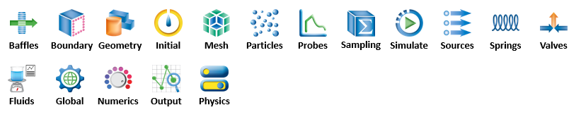
New Model Setup icons

새로운 모델 설정 디자인에는 설정 프로세스의 각 단계를 나타내는 새로운 아이콘이 있습니다.

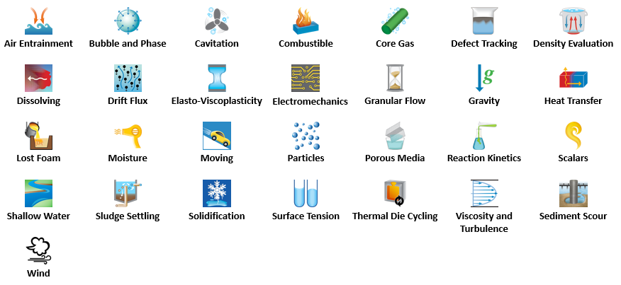
New Physics icons

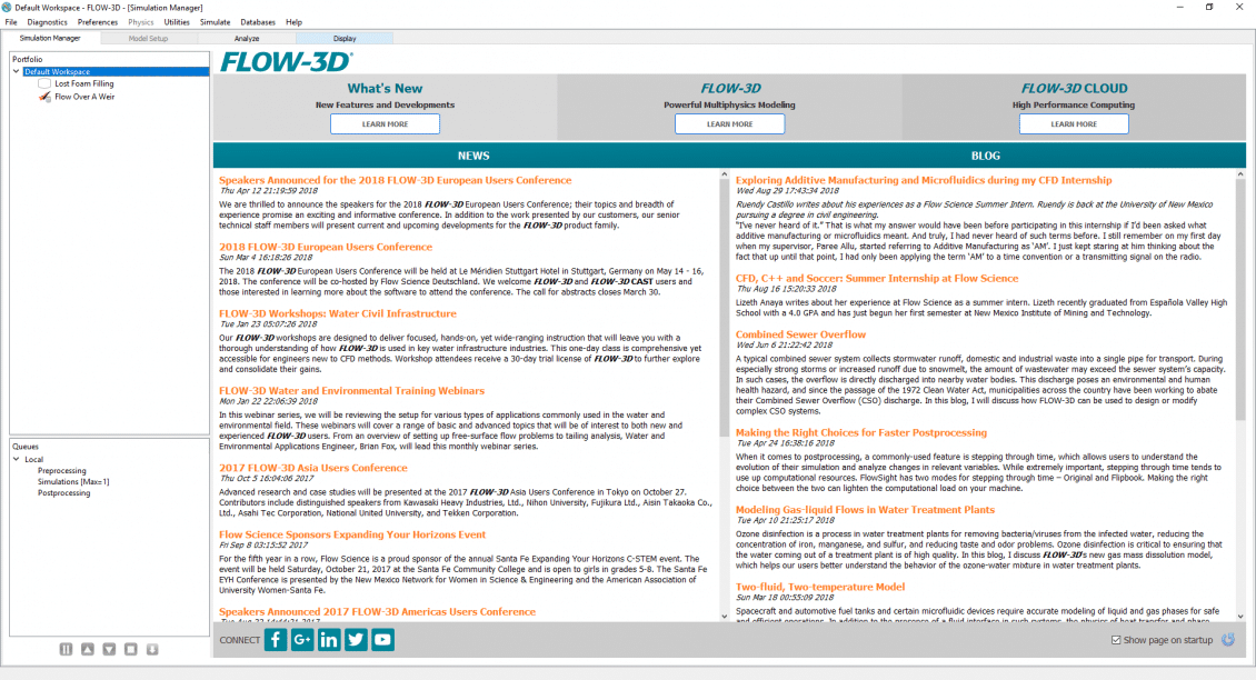
RSS feed

새 RSS 피드부터 FLOW-3D v12.0의 시뮬레이션 관리자 탭이 개선되었습니다. FLOW-3D 를 시작하면 사용자에게 Flow Science의 최신 뉴스, 이벤트 및 블로그 게시물이 표시됩니다.

Configurable simulation monitor

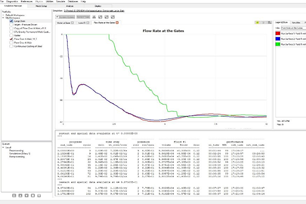
시뮬레이션을 실행할 때 중요한 작업은 모니터링입니다. FLOW-3Dv1.0에서는 사용자가 시뮬레이션을 더 잘 모니터링할 수 있도록 SimulationManager의 플로팅 기능이 향상되었습니다. 사용자는 시뮬레이션 런타임 그래프를 통해 모니터링할 사용 가능한 모든 일반 기록 데이터 변수를 선택하고 각 그래프에 여러 변수를 추가할 수 있습니다. 이제 런타임에서 사용할 수 있는 일반 기록 데이터는 다음과 같습니다.

최소/최대 유체 온도
프로브 위치의 온도
유동 표면 위치에서의 유량
시뮬레이션 진단(예:시간 단계, 안정성 한계)

Runtime plots of the flow rate at the gates of the large dam

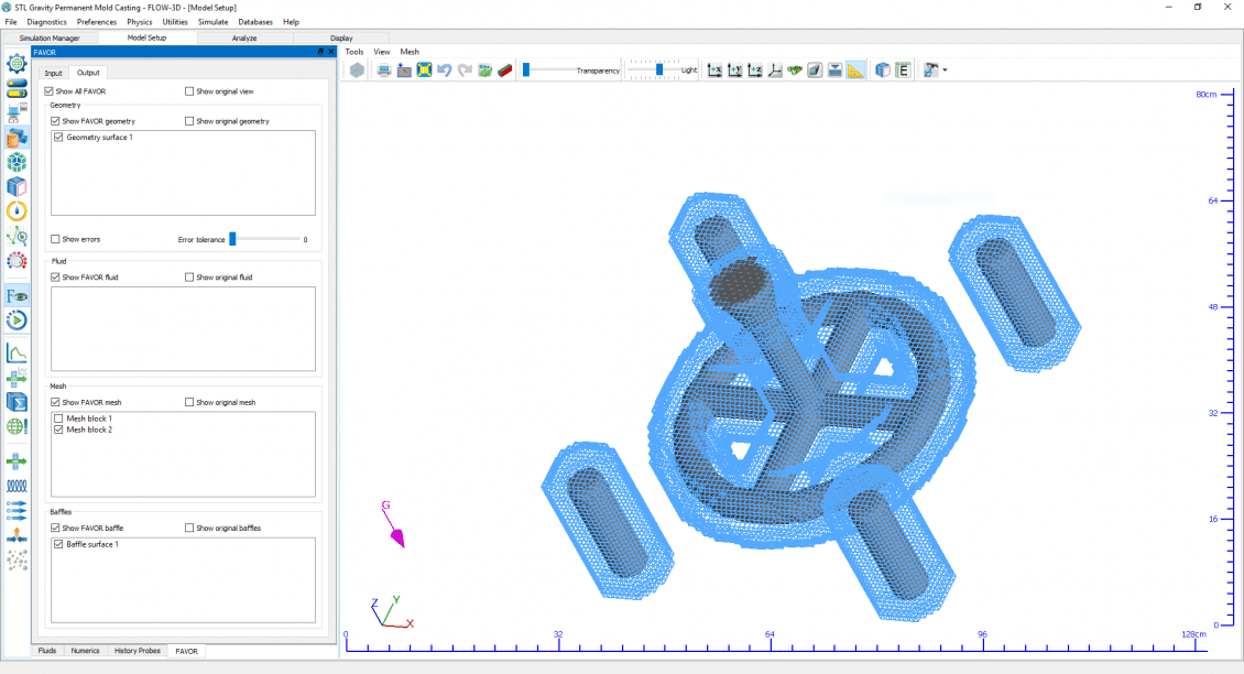
Conforming 메쉬 시각화

용자는 이제 새로운 FAVOR ™ 독 위젯을 통해 적합한 메쉬 블록을 시각화 할 수 있습니다.

Large raster and STL data

데이터를 처리하는 데 걸리는 시간 때문에 큰 지오 메트리 데이터를 처리하는 것은 수고스러울 수 있습니다. 대형 지오 메트리 데이터를 처리하는 데는 여전히 상당한 시간이 걸릴 수 있지만, FLOW-3D는 이제 이러한 대규모 데이터 세트를 백그라운드 작업으로 로드하여 사용자가 데이터를 처리하는 동안 완전히 응답하고 중단 없는 인터페이스에서 작업을 계속할 수 있습니다

스크류 펌프 유동해석관련 사례 및 자료

스크류 펌프 유동해석관련 사례 및 자료입니다.

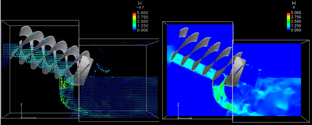
소규모 수력 발전소의 사용은 증가하는 에너지 비용을 통제하는 방법으로 더욱 흥미롭게 연구되고 있습니다. 전통적인 대형 수력 발전소는 규제 검토를 위해 막대한 자본 투자와 긴 리드 타임을 필요로합니다. 더 작은 발전소는 새로운 유형의 터빈을 사용할 수 있습니다. FLOW-3D를 통해 아르키메데스 이송 나사의 원리에 따른 유동현상을 유체 역학을 통해 분석할 수 있습니다.

홈페이지 관련 내용 https://www.flow3d.com/hydrodynamic-screws/

해석사례 동영상 1 https://www.youtube.com/watch?v=z2NrkY57ZHU

해석사례 동영상 2 https://www.youtube.com/watch?v=ajMhH0i3lwM

MODERN HORIZONTAL AXIS ARCHIMEDEAN WATER CURRENT TURBINES

[FLOW-3D 물리모델] Solidification 응고

응고 모델은 열전달이 활성화되고(Physics → Heat Transfer → Fluid internal energy advection) 유체비열(Fluids → Fluid 1 → Thermal Properties → Specific heat)과 전도도(Fluids → Fluid 1 → Thermal Properties → Thermal Conductivity) 이 지정될 때 사용될 수 있다. 단지 유체 1만 상 변화를 겪을 수 있다.

응고모델을 활성화하기 위해 Fluids → Fluid 1 → Solidification Model 을 체크하고 물성 Fluids → Fluid 1 → Solidification Model 가지에서 Liquidus temperature, Solidus temperature, 그리고 Latent heat of fusion 를 지정한다. 가장 간단한 모델(Latent Heat Release Definition 에 펼쳐지는 메뉴에서 Linearly with constant 를 선택)에서, 잠열은 물체가 Liquidus 에서 Solidus 온도로 냉각될 때 선형적으로 방출된다. 고상에서의 상변화열을 포함하는, 잠열 방출의 더 자세한 모델을 위해 온도의 함수로 잠열방출을 정의하기 위해 Specific energy vs. temperature 또는 Solid fraction vs. temperature 선택을 사용한다. 이 지정에 대한 더 자세한 내용은 이론 매뉴얼의 Heat of Transformation 를 참조한다.

응고는 유체의 강직성 및 유동저항을 뜻한다. 이 강직성은 두 가지로 모델링 된다. 낮은 고상율에 대해 즉 Fluids → Fluid 1 → Solidification Model → Solidified Fluid 1 Properties → Coherent Solid Fraction 의 coherency 점 밑에서는 점도는 고상율의 함수이다. 간섭 고상율보다 큰 고상율에 대해서는 고상율의 함수에 비례하는 항력계수를 갖는 Darcy 형태의 항력이 이용된다. 이 항력은 모멘텀 방정식에 (b_x,b_y,b_z) 로써 추가된다- Momentum Equations 를 보라. 이 항력의 계산은 Solidification Drag Model 에서 기술된다. 항력계수는 사용자가 유동저항에 양을 조절할 수 있는 Coefficient of Solidification Drag 인자를 포함한다. 항력계수는 FLOW-3D 출력에서 기록된 속도에 상응하는 지역 상 평균 속도에 의해 곱해진다.

Fluid 1 Properties)을 지나면 항력은 무한대가 되고 계산격자 관련하여 유동이 있을 수 없다(단 예외로 Moving Solid Phase를 참조).

Note

모든 유체가 완전히 응고하면 모사를 정지시키기 위해 General → Finish condition → Solidified fluid fraction 를 이용한다. General → Finish condition → Finish fraction 은 모사를 중지하기 위한 고상율 값을 정한다.

Drag in the Mushy Zone, Mushy영역 내 항력

주조 시 mushy zone 은 액상과 고상이 혼합물로 존재하는 지역이다. 이 지역 혼합점도는 동축의 수지상 조직(과냉각된 액체 안에서 방사상으로 자라는 결정으로 된 구조) 이 액체 안에서 자유롭게 부유할 때 영향을 미친다.

일단 수지상 조직의 간섭성이 발생하여 고정된 고상 망이 형성되면 액상이 고정된 다공 수지상 구조를 통과해야 하므로 추가의 유동손실이 발생한다. 다른 방법으로는 간섭점을 지난 액/고상 혼합물은 다공물질을 통한 유동 대신에 고점도의 유체로 간주될 수 있다. 점성유체로 간주하는 접근은 예를 들면 연속 이중 롤 주조 과정같이 고상이 계속 이동 및 변형할 때 유용하다.

Solidification Drag Models in FLOW-3D, FLOW-3D 내 응고 항력모델

응고에 의한 항력계수를 정의하기 위해 사용자는 우선 열전달 및 응고모델을 활성화 해야 한다. 이들은 Model Setup → Physics 탭 에서 활성화될 수 있다. 수축모델 또한 응고모델 창에서 활성화될 수 있다.

일단 Solidification 모델이 활성화되면 항력의 공식이 지정될 필요가 있다. Solidification대화의 밑 좌측 모퉁이에서 Porous media drag-based 와 Viscosity-based 의 항력공식 중의 선택을 한다.

- Viscosity-based 공식은 점성 유체로 취급하며 Viscosity 영역 내Flow model for solidified metal 입력 밑에서 지정되는 순수 고상 점성을 갖는 고상화된 유체로 간주된다. 이 접근법은 경직성의 항력모델(즉, 응고 금속이 롤러 사이로 압착될 때)을 사용할 수 없는 경우의 모사에 이용된다. 이 점성은 고상율에 따라 선형으로 변한다.고상율이0일 때 점도는 유체1의 점도이다.고상율이1이면 점도는 Solidification 패널에서 지정된 값과 같다.
- Porous media drag-based 공식은 응고상태를 결정하기 위해 고상율을 사용한다. 고상율이 Critical Solid Fraction 이거나 초과하면 이때 항력은 무한대가 된다-즉, 액상/고상 혼합물은 고체같이 거동한다. 고상율이 Coherent Solid Fraction 보다 작으면 항력은 0이다. 이 두 값 사이에서 유동은 mushy 지역에 있고 이를 통한 유동은 마치 다공질 내에서의 유동같이 처리된다. 또한 모델은 고상율이 Coherent Solid Fraction 보다 작을 때 자동적으로 용융 금속의 점도를 조절한다. 이 상태에서 고상결정은 점도를 올리지만 결합하지는 않는다(즉, 간섭 없음). 일단 유체가 Coherent Solid Fraction 에 도달하면 항력방정식이 고려되고 점도는 간섭성에 도달하기 전의 값으로 일정하게 된다. 임계 및 간섭 고상율은 사용자가 정의하며 논문이나 책 등에서 찾을 수 있다. 이 식에서는 Coefficient of Solidification Drag 가 정의되어야 한다. 이는 Solidification 창 또는 Fluid 1 → Solidification Model→Solidified Fluid 1 Properties tree → Other 트리를열어 Model Setup →Fluids 탭에서 될 수 있다.

How to Calculate Permeability 투과성 계산법

밑에 주어진 Darcy법칙은 수지상 구조를 위한 다공매질내의 수학적 유동기술이다.[Poi87].

(19) $\mathbf{u} = - \frac{K}{\mu} \nabla P$

여기서 u 는 수지상 구조 내 유동의 속도이고 ∇P 는 지역 압력구배, 그리고 K 는 mushy 구역의 특정 투수성이다. 이 방정식은 단지 유동이 거의 정상 상태이고, 관성효과가 없으며 유체의 체적율이 일정하고 균일하며 액체-액체의 상호작용 힘이 없을 때 유효하다. 투수성을 정의하는데 이용될 수 있는 대 여섯 개의 모델이 있으나 FLOW-3D 는 밑에 보여주는 Blake-Kozeny 을 이용한다. 다른 모델들은 코드와 함께 제공되는 소스코드를 사용자 사양에 맞게 수정하여 추가할 수 있다.

(20) $\mathbf{u} = -C_2 \left( \frac{\lambda_1^2 (1-f_s)^3}{\mu f_s^2} \right) \left( \nabla P - \rho \mathbf{g} \right)$

여기서

C₂는 전형적으로 와 같은 비틀림

f_s는 고상율이고

λ₁는 유동을 위한 특정 치수

이 응용에서 수지상 가지 간격(DAS)이 이용된다.

식 (11.19) 을 식(11.20) 에 적용하면 투수성을 위한 다음 식을 얻는다.

(21) $K = \lambda_1^2 \frac{(1-f_s)^3}{180f_s^2}$

수지상 가지 간격(DAS)에 대한 일반적인 값들은 밑에 주어져 있다.

Range of Cooling Rates in Solidification Processes¶
COOLING RATE, K/s	PRODUCTION PROCESSES	DENDRITE ARM SPACING, $\mu m$
$10^{-4}$ to $10^{-2}$	large castings	5000 to 200
$10^{-2}$ to $10^3$	small castings, continuous castings, die castings, strip castings, coarse powder atomization	200 to 5
$10^3$ to $10^9$	fine powder atomization, melt spinning, spray deposition, electron beam or laser surface melting	5 to 0.05

Range of cooling rates in solidification processes [CF85]

How FLOW-3D Defines the Coefficient of Solidification Drag FLOW-3D 가 응고 항력계수를 결정하는법

FLOW-3D 는 액고상 변화를 모델링하기 위해 다공매질항력을 이용한다. 항력은 고상율의 함수이다. 사용자에게 두 수축모델이 이용 가능하다; 급속 수축 모델 과 완전 유동모델. 급속 수축 모델은 상변화와 연관된 체적변화를 고려하지 않으며 유체는 정지해 있다고 가정한다. 완전 유동모델은 상변화가 관련된 체적변화를 고려한다. 항력은 투수성에 역으로 비례하므로 다음과 같이 표현될 수 있다.

(22) $K = \frac{\mu}{\rho F_d}$

여기서, F_d는 FLOW-3D 에서 사용된 항력계수이다. 이 항력계수는 지역 속도에 의해 곱해지고 모멘텀 방정식의 오른쪽에서 차감된다 (Momentum Equations 참조). 식 (11.22) 를 재정리하고 식 (11.21) 로부터의 투수성에 치환하면 다음을 얻는다.

The Coefficient of Solidification Drag: $\text{TSDRG}=\frac{180 \mu}{\lambda_1^2\rho }$ ,
The drag force: $F_d = \mbox{TSDRG} \frac{ f_s^2}{(1-f_s)^3}$ .

Macro-Segregation during Alloy Solidification 합금응고시 거시적 편절

편절 모델은 대류와 확산에 의한 용질 이동에 따른 이원합금 요소에서의 변화를 모델링 하도록 되어 있다. 이 모델링은 Physics → Solidification 로 부터 될 수 있다.

Activate binary alloy segregation model 을 체크하고 편절 모델을 활성화한다.

여러 온도에서 평형에 있는2원합금 요소농도를 정의하는 상태도는 직선의 고상선 및 액상선을 가진다고 가정된다. 상태도는 입력데이터에 의해 구성되고 전처리 그림파일 prpplt 에 포함된다. Analyze → Existing 에서 이용 가능하다

Macro-Segregation Model (under Fluids → Fluid 1 → Solidification Model)에 관련된 일부 유체물성 트리가 밑에 보여진다. 상태도는 Reference Solute Concentration 에서의 the Solidus 와 Liquidus Temperatures 값들에 의해 정의된다. 추가로 Concentration Variables 밑의 Partition coefficient 도 정의되어야 한다. 그렇지 않으면 Pure Solvent Melting Temperature 가 정의될 수 있다. Partition coefficient 와 Pure Solvent Melting Temperature 둘 다가 지정되면 용매 용융 온도는 상태도로부터 재 정의된다.

Eutectic Temperature 또는 Eutectic Concentration 는 융해작용을 정의하기 위해 지정될 수 있다. 또 이 두 변수가 다 지정되면 Eutectic Concentration 은 상태도에서 재 정의된다.

Diffusion Coefficients 는 고상과 액상 사이의 용질의 확산계수 비율을 정의한다. 액체 내의 용질의 분자 확산계수는 Physics → Solidification 에서 specifying Solute diffusion coefficient 를 지정함으로써 정해진다. RMSEG 는 용질의 난류 확산계수 승수를 정의한다; 이는 입력파일에서 직접 지정된다.

용질 재 분배에 의한 농도변화가 중요하면 Physics → Density evaluation → Density evaluated as a function of other quantities를 정하고 용질농도의 선형함수로써 금속농도를 정의하기 위해 Fluids → Segregation model 밑의 Solutal Expansion Coefficient 를 용질 확장계수로 지정한다. 이 경우 Reference Solute Concentration 이 기준농도로 사용될 것이다. 추가로 Fluids → Fluid 1 → Density Properties → Volumetric Thermal Expansion 은 액체 내 열부력 효과를 참작하기 위해 지정될 수 있다(또한 Buoyant Flow참조).

초기 용질농도는 Meshing & Geometry → Initial → Global → Uniform alloy solute concentration 에서 지정될 수 있다. 불 균일한 초기 분포는 Alloy solute concentration 밑의 초기유체 구역 안에서 정의될 수 있다. 추가로 농도는 Initial Conditions: Region Values 에서 기술된 바와 같이 2차함수를 사용하는 부분을 편집하여 공간상의2차함수로 변화할 수 있다. 압력과속도 경계에서 용질 경계조건을 정하기 위해 Boundaries → Boundary face → Solute concentration 를 이용한다.

액상 및 고상 구성은 후처리에서 데이터 변환을 이용하여 그려질 수 있다. 용융 응고금속은 금속 내 용융의 질량 분율을 저장하는 SLDEUT 를 그림으로써 가시화될 수 있다.

액상 내 열구배가 크면 Physics → Heat Transfer → Second order monotonicity preserving 를 지정함으로써 더 나은 정확성을 위해 고차원 이류법을 사용한다.

mushy 지역에서의 유동손실은 수지상 가지 간격(DAS)의 함수인 Fluids → Fluid 1 → Solidification Model → Solidified Fluid 1 Properties → Coefficient of Solidification Drag 에 의해 조절된다. 후자는 이 모델에 의해 계산되지 않으므로 사용자는 Coefficient of Solidification Drag 를 지정해야 한다

Note

표준 응고모델 과는 달리 상태도상의 용융점을 지나 고상선을 외삽하여 정의되므로 여기서 응고선의 값은 음수일 수 있다.

Microporosity Formation 미세다공형성

미세다공모델은 단지 응고(Solidification참조)를 모델링할 때 사용될 수 있고 Physics → Solidification → Activate micro-porosity model 에서 활성화된다. 필요한 입력은 Fluids → Densities → Fluid 1 and Fluids → Solidification Properties → Solidified Fluid 1 Properties → Density 에서 정의되는 액체와 고상 유체밀도이며 고상유체밀도는 액체밀도보다 크다. 또한 Fluids → Fluid 1 → Solidification Model → Solidified Fluid 1 Properties 안에 있는 Critical Solid Fraction 은 1.0보다작게 설정되어야 한다.

Square of the speed of sound at critical solid fraction 값이 정의될 수 있다. 이는 수축에 의해 mushy 지역에서 전개되는 커다란 음압에서의 응고유체의 압축성을 기술한다. Critical pressure at which gas pores can form 값은 모델이 Initial tab 탭에서 또는 재 시작 데이터에서 정의되는 유체내의 초기 압력과 결합되도록 한다.

Intensification pressure 또한 다공 생성을 지연시키기 위해 응고 시 shot sleeve plunger 에 의해 형성되는 추가압력을 고려하기 위한 고압 주조모사를 위해 정의될 수 있다. Intensification pressure 가 클수록 더 적은 양의 다공이 주조 시 응고 과정에서 발생할 것이다.

미세 다공 모델은 응고 모델의 활성화 이외의 어떤 다른 설정을 필요로 하지 않는다. 이는 완전 유동방정식이나 속도장이 0인 경우, 즉 순수한 열 문제에서도 함께 사용될 수 있다.

이 모델은 후처리 과정의 공간 및 이력에서 사용 가능한 Percent micro-porosity 라고 불리는 추가 출력 양을 생성한다.

Note

A Flow Science technical note on modeling micro-porosity (TN66) can be found at http://users.flow3d.com/technical-notes/.

Moving Solid Phase 이동고상

MAIN VARIABLES:

OBS:

IFOB, UTOBS, VTOBS, WTOBS

이동고상 선택은 연속주조 모델링을 가능하게 한다. Continuous Casting Phantom 요소는 응고된 이동 유체가 있는 지역에서 정의된다. 이는 지정된 영역을 차지하지만 정의에만 존재하므로 환영요소라고 한다. 이는 실제로 면적이나 체적을 차지하지 않으므로 체적이 없고 결과에서도 고체요소로 보이지 않는다. 이는 Meshing & Geometry → Geometry → Component → Component Type 옆 펼쳐지는 메뉴에서 정의된다.

다른 방법으로는 입력파일(prepin.*)에서 IFOB(N) 변수가 4로 지정되고 N 은 요소 번호이다. 이 파일은 File → Edit Simulation…. 을 선택하여 이용될 수 있다. 또한 입력파일에서 시간의 함수(TOBS(t) 에 의해 지정되는)일 수 있는 가상 요소의 속도성분 UTOBS(t,N), VTOBS(t,N) 그리고 WTOBS(t,N) 이 지정된다.

Fluids → Fluid 1 → Solidification Properties → Solidified Fluid 1 Properties → Coherent Solid Fraction 에 의해 정의된 간섭 고상율 보다 큰 고상율에 대해서는 Darcy 형태의 항력 이 유체를 가상 요소의 속도로 움직이게 하는데 사용된다. 고상율이 Fluids → Fluid 1 → Solidification Properties → Solidified Fluid 1 Properties → Critical Solid Fraction 에서 지정된 경직점을 능가하게 되면 가상 요소의 속도를 따라 움직일 것이다.

Note

가상 요소는 요소 그림에 안 나타나나 Component number 를 그릴 때는 보여진다.가상 요소는 균일속도가 요소의 전체에 적용되므로 평평해야 한다.

Solidification Shrinkage 응고수축

체적 수축은 소재가 응고하고 응고소재의 밀도가 액체소재의 밀도보다 클 때 나타난다(즉, Fluids → Fluid 1 → Solidification Model → Solidified Fluid 1 Properties → Density > Fluids → Fluid 1 → Density Properties → Density). 수축모델은 그러므로 Solidification 모델이 활성화되어야 하고 고상/액상의 두 밀도가 정의되어야 한다. 수축은 단지 1유체의 뚜렷한 경계면 문제에서만 모델링 될 수 있다.

두 가지 수축모델이 있다. Shrinkage model with flow effects 를 선택하면 완전 열 유체방정식을 해석한다(이론 매뉴얼의Solidification Shrinkage and Porosity Models 참조). 그러나 이 모델은 특히 장시간의 응고가 고려되면 컴퓨터 계산시간이 많이 소요된다. 다른 방법으로 사용자 Interface 에 Shrinkage model 이라고 불리는 단순모델이 있다.

이 모델은 단지 열전달 방정식의 해석에 의존하며 특히 내재적 열전달 모델 (Numerics → Explicit/implicit options → Heat transfer → Implicit –Thermal solution 참조)과 사용시에 빨리 해석할 수 있다. 액체 체적 내로의 유동 통로가 없을 때 내부공동이 발생한다.

이 두 모델에서 유입은 mushy 지역 유동에 대한 항력계수를 계산함으로써 정의된다. 격자 내 모든 점에서의 항력함수는 상수승수 Fluids → Solidification properties → Other → Coefficient of Solidification Drag (Solidification Drag Model 참조)를 가지는 지역 고상율의 함수로 계산된다. 항력함수의 역의 값은 공간 그림에서 가시화 될 수 있다: 이 그림을 위한 변수이름은 ‘drag coefficient’ 이다.

Mushy 지역에서의 커다란 유동 손실에 따른 부분적 유입이 Shrinkage model with flow effects 에서 발생할 수 있지만 단순화된 Shrinkage model 은 완전 유입이 아니면 유입이 없게 된다. 후자는 유입 통로를 따라 지역 고상율이 Fluids → Fluid 1 → Solidification Model → Solidified Fluid 1 Properties → Critical Solid Fraction (디폴트는1.0)에서 정의된 임계값보다 커질 때 발생한다. 추가로 고립된 액체 내의 금속의 고상율이 Coherent Solid Fraction 에 도달할 때까지 단순모델에서의 유입은 고립부 상부로부터 발생한다. 그 후로는 유입이 고립부의 가장 뜨거운 부분에서부터 발생한다.

모든 유체가 완전히 응고되면 모사가 정지하도록 General → Additional finish condition → Solidified fluid fraction 를 사용한다. 변수 Finish fraction 는 유체가 지정된 고상율에 도달할 때 모사가 정지하도록 하는데 사용될 수 있다.

$Solid fraction finish condition$

Note

이송 방향을 결정하기 위해 단순 수축 모델에서 중력이 필요하며 좌표축 중 하나를 따라야합니다. 둘 이상의 중력 구성 요소가 0이 아닌 경우, 가장 큰 중력 구성 요소가 공급 방향을 결정하는 데 사용됩니다.

액티브 시뮬레이션 제어

전산 유체 역학 (Computational fluid dynamics, CFD)은 설계자가 개발하고자 하는 시나리오를 설계 할 수 있는 가상 실험실을 제공함으로써 오랫동안 제품 개발에 중요한 역할을 해왔습니다.

일반적으로 사용자는 수치해석을 통해 제품 설계 및 성능 검토를 위해서 시뮬레이션을 합니다. 성능 검증을 위해 일반적으로 기하학, 재료 특성 및 질량 유량, 경계 온도 및 압력, 출력 빈도와 같은 유동 조건이 포함됩니다. 시뮬레이션에서 얻은 결과 정보를 기반으로 다양한 입력 조건을 수정하고 더 많은 가정 시나리오를 조사하기 위해 시뮬레이션을 다시 시작합니다.

시뮬레이션에 대한 이러한 접근 방식은 폐회로 제어와 유사한 “what if – then do this”라고 생각할 수 있습니다. Active – Simulation Control이라고 불리는 FLOW-3D 및 FLOW-3D Cast 버전의 새로운 기능은 사용자들에게 인상적인 “what if – then do this” 컨트롤에 대한 시뮬레이션을 제공합니다.

용어 – 이벤트/조건 및 조치

능동적인 시뮬레이션 제어는 이벤트/조건 및 동작이라는 두 가지 개념을 기반으로 합니다. 다음은 각각에 대한 간단한 설명입니다.

이벤트/조건

히스토리 프로브의 사용자 지정 조건이 충족되면 이벤트가 발생합니다. 모든 유형의 프로브(정적 프로브, GMO에 부착 된 프로브 및 FSI / TSE 프로브)를 사용하여 조건을 정의 할 수 있습니다. 이벤트는 1-10 개의 조건으로 구성 될 수 있습니다. 사용자는 이벤트가 발생하기 위해 조건 중 하나 또는 모두를 충족해야하는지 여부를 지정할 수 있습니다.
조건의 예는 다음과 같습니다.

히스토리 프로브 # 1의 유속은 3.25 미터 이상입니다.
히스토리 프로브 # 2의 압력이 1 기압 미만
지정된 조건이 충족되면 이벤트가 발생하고 이벤트와 연관된 모든 동작이 활성화됩니다.

행위

동작은 이벤트가 발생할 때 활성화되는 시뮬레이션에 대한 사용자 정의 변경입니다. 각 이벤트는 하나 이상의 조치를 활성화 할 수 있습니다. 동작의 몇 가지 예는 다음과 같습니다.
y 축에 대한 GMO 회전을 외부 파일에 정의 된 시간 종속 값으로 설정합니다.
메쉬 블록 1의 x-min 경계에서 y- 속도를 0.0으로 설정합니다.
선택된 데이터 출력의 빈도를 0.0으로 설정하십시오 (매 사이클 출력)

응고 시뮬레이션에서 스퀴즈핀 활성화

이벤트가 발생하면 이벤트에 지정된 모든 동작이 활성화됩니다.

능동 시뮬레이션 제어의 응용

고압 다이 캐스팅

샷 플런저를 고속 샷으로 전환 : 고압 다이캐스팅 머신의 샷 플런저의 초기 동작은 공기 유입을 최소화하도록 제어됩니다. 예를 들어, 금속이 게이트에 도달하면 샷 동작이 빠른 샷으로 전환되어 부품의 금속을 원자화합니다. 능동적인 시뮬레이션 제어는 금속이 게이트의 일부 또는 전부에 도달했을 때 이를 감지하고 이에 따라 플런저 동작을 변경하는 데 사용할 수 있습니다.

중력 주조

중력 주조는 종종 쏟아져 나오는 분지를 사용하여 일정한 압력 헤드가 스프 루 위에 유지되도록합니다. 액티브 시뮬레이션 제어는 유역의 유체 높이를 기반으로 유역으로 붓는 것을 제어하는 데 사용할 수 있습니다.

물 / 환경

제어 게이트는 어류가 받아 들일 수 있는 범위로 유속을 제한하기 위해 댐 구조물을 통과하는 어류 통로에서 일반적으로 사용됩니다. 능동적 시뮬레이션 제어는 물고기가 있는 지역에 위치한 프로브에서 속도 정보를 기반으로 게이트를 이동시키는 데 사용할 수 있습니다.

항공 우주

극저온 연료 탱크의 압력은 적절한 작동 및 안전을 보장 할 수 있도록 설계단계에서 유지되어야합니다. 순압력흡입헤드가 허용 수준 이하로 떨어지면 엔진에서 캐비테이션이 발생하고 장치가 파괴 될 수 있습니다. 능동적 시뮬레이션 제어는 증기 공간에서의 압력(이력 프로브) 손실에 대한 시스템의 가압 (질량 운동량 소스) 및 감압 (밸브 개방)을 시뮬레이션하는데 사용할 수 있습니다.

능동 시뮬레이션 제어 데모

능동적인 시뮬레이션 제어는 충진 켜기/끄기 및 믹서 동작을 제어하기 위해 혼합 시뮬레이션에 적용 할 수 있습니다 (아래 참조). 수축 충진관을 사용하여 용기에 마커 염료가 함유된 유체를 채웁니다. 충전이 완료되면 패들 믹서가 용기 내로 내려갑니다.

프로브가 필러 튜브에 부착되어 위치를 감지합니다. 다른 프로브가 믹서의 바닥에 부착되어 그 위치를 감지합니다.

필러 튜브가 지정된 레벨 이상으로 상승하면 혼합 임펠러가 유체로 들어가기 시작합니다. 믹서가 지정된 레벨에 도달하면 회전이 시작됩니다. 믹서가 콘테이너의 바로 위에있는 포인트에 도달하면, 믹서는 아래로 이동하는 것을 멈추지만 계속 회전합니다.
아래의 애니메이션은 컨테이너를 채우고 혼합할 때 유체의 염료 농도를 보여줍니다.

결론

여기에 표시된 믹싱 예제는 활성 시뮬레이션 컨트롤이 제공하는 광범위한 기능을 보여줍니다. 능동적인 시뮬레이션 제어를 통해 사용자는 설계의 실제 동작을보다 자세하게 표현할 수 있으며 시뮬레이션을 재시작하지 않고도 시뮬레이션 변경 사항을 적극적으로 구현할 수 있습니다.

열응력 개선 / Thermal Stress Evolution

FLOW-3D의 TSE(Thermalstressdiversion)모델은 모델링 가능한 주조 프로세스의 범위를 확장합니다. FSI/SETSE모델은 주변 유체, 열 구배 및 지정된 구속 조건의 압력에 대응하여 솔리드 및 단단한 구성 요소의 응력 및 변형을 모델링 하는 유한 요소 접근 방식을 사용하여 유체와 솔리드 사이의 완전 결합 상호 작용을 설명합니다.

균일하지 않은 냉각에 의해 발생하는 응고 과정 동안 열 스트레스가 발생합니다. 이러한 응력은 주형 벽의 수축 및 주물 형상의 불규칙에 의해 영향을 받습니다.
Von Mises stresses in a solidified aluminum V6 engine block

위의 시뮬레이션은 VonMises가 단단한 알루미늄 V6엔진 블록에서 응력을 나타냅니다. 이 블록은 강철 다이 내에서 주조된 알루미늄 A380합금으로 구성되어 있습니다.

알루미늄의 주입 온도는 527°C였으며 초기 다이 온도는 125°C였습니다. 부품을 60초 동안 다이 내에서 냉각한 후 주변 조건(125°C)에서 9분 동안 부품을 계속 냉각시켜 총 10분의 시뮬레이션 시간을 제공했습니다. 표시된 VonMises 응력은 부품 내 전단 응력의 크기를 측정한 것이며, 따라서 찢어지기 쉬운 부위를 보여 줍니다.

응력은 금형과 응고 금속에서 동시에 계산할 수 있습니다. FLOW-3D의 구조화된 메쉬를 초기 템플릿으로 사용하여 자동으로 메쉬 작업을 수행할 수 있습니다. 사용자는 중첩 또는 링크된 메쉬 블록을 만들고 V1.1.0의 새로운 적합한 메쉬 기능을 사용하여 메쉬의 로컬 해상도를 제어할 수 있습니다. 또는, Exodus-II형식의 타사 메쉬 생성 소프트웨어에서 유한 요소 메쉬를 가져올 수 있습니다.

Simulating Thermal Stress

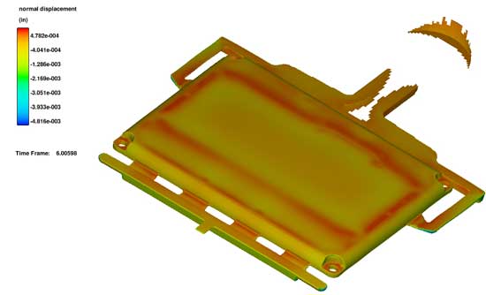
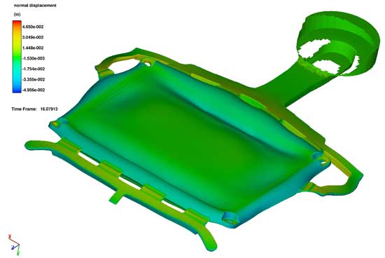
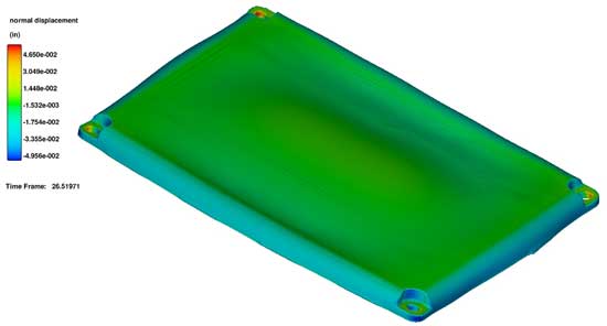
아래에 표시된 알루미늄 커버는 강철 다이 내 알루미늄 A380합금으로 구성되어 있습니다. 주입 온도는 654°C였으며 초기 다이 온도는 240°C였습니다. 부품이 다이 내에서 6s동안 냉각되었으며 이때 부품이 완전히 경화되었습니다(러너 시스템 제외). 그런 다음 다이를 열고 부품이 주변 조건(25°C)에서 10초 이상 냉각되도록 했습니다. 그런 다음 탕도(runner)시스템을 제거했고, 이후 주변 조건에서 10초간 더 냉각했습니다. 여기에 표시된 정상 변위는 부품 표면의 움직임을 나타내며, 최대 변형 영역을 강조하기 위해 30회 증폭됩니다.

Displacements in a die cast part, die closed.

Displacements in the part and runners, die open.

Displacements in the part with runner system removed.

Component Coupling within the Fluid-Structure Interaction and Thermal Stress Evolution Models

FLOW-3Dv11의 새로운 기능은 인접한 FSI(유체-구조물 상호 작용)구성 요소 및/또는 TSE(열 스트레스 진화)고체화된 유체 영역 간의 탄성 응력을 결합할 수 있는 기존의 유한 요소 고체 역학 용제의 업그레이드입니다. 이 새로운 기능은 복합 재료 부품(예:주형에서 응고되는 금속 주물 응고제 또는 바이메탈 게이지)의 열 응력과 변형을 시뮬레이션하고 반경 게이트 및 파이프 라인 지지 시스템과 같은 연결된 유압 구조에 가해지는 힘을 시뮬레이션하는 등 다양한 모델링 가능성을 열어 줍니다.

모델에는 복잡한 프로세스를 효율적으로 계산할 수 있는 여러가지 옵션이 있습니다.

No coupling

이 옵션은 인접 FSI구성 요소가 응력을 교환하지 않는 단순화된 경우를 나타냅니다. 그것은 계산적으로 효율적이며 요소들 간의 스트레스 상호 작용이 중요하지 않은 시나리오에 적합하다.

Full coupling

전체 커플링 옵션은 서로 다른 재료 특성을 가진 인접 FSI구성 요소를 모델링 하기 위한 것입니다. 두 구성 요소는 서로 당기거나 미끄러질 수 없지만 인터페이스의 응력은 구성 요소 간에 전달됩니다. 이는 바이메탈과 같이 접합된 구조물을 모델링 하는 데 이상적입니다.

Partial coupling

부분 커플링 옵션은 인접 FSI구성 요소가 마찰력과 정상적인 힘을 통해 상호 작용하지만 분리될 수 있는 일반적인 문제를 모델링 하기 위한 것. 이 옵션은 FSI구성 요소와 TSE의 고체화된 유체 영역을 결합하는 데 사용될 수 있으므로 부품이 다이에서 냉각될 때 주조 부품 및 다이에 대한 열 응력의 영향을 조사하는 데 이상적입니다.

두가지 시뮬레이션이 제시되어 모델의 새로운 특징을 보다 자세히 보여 줍니다. 첫번째 상황에서는 완전한 커플링 옵션을 사용하여 시간이 변화하는 온도에 대응하여 바이메탈 벤딩을 모델링 하는 반면, 두번째 예에서는 다이에서 V6엔진 블록을 응고하는 동안 부분 커플링 모델을 사용하여 열 응력을 확인하는 것을 보여 줍니다.

Full Coupling Example: Bimetallic Strip

전체 커플링 옵션의 가장 간단한 예 중 하나는 온도 구배에 대한 반응으로 바이메탈이 움직이는 것입니다. 이러한 스트립은 온도 변화에 대응하여 두 금속이 동일한 속도로 팽창하지 않기 때문에 열 스위치 및 벤딩에 일반적으로 사용됩니다. 시뮬레이션에서 모델링 된 바이메탈은 그림 1과 같이 길이 15cm, 두께 0.5cm의 강철 스트립으로 구성된 캔틸레버 빔입니다.

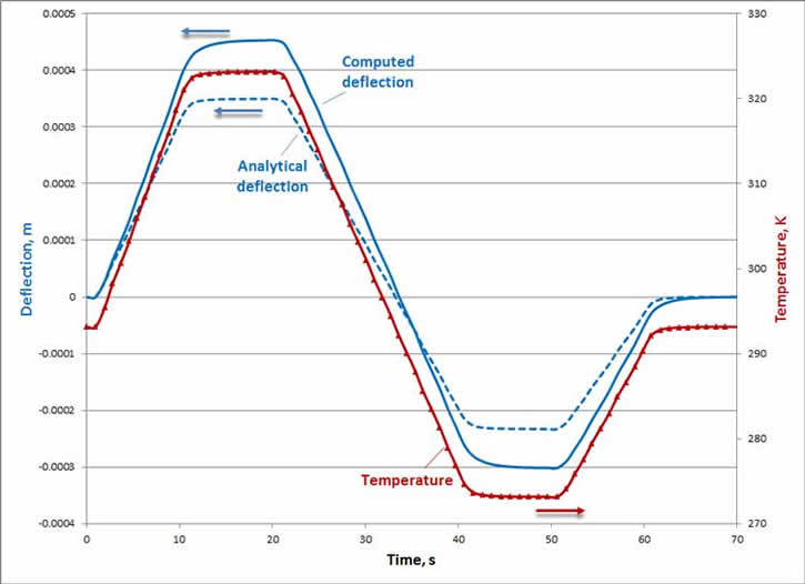
그리고 나서 스트립은 온도가 70초에 걸쳐 균일하게 변화하는 환경에 배치되었다. 그림 2는 시간 경과에 따른 다양한 온도에서 시뮬레이션 및 분석 용액을 위한 스트립 팁의 편향을 보여 준다. 결과는 온도가 변한 시기와 스트립의 열적 관성으로 인한 스트립의 반응 사이의 약간의 지연을 포함하여 몇가지 흥미로운 특징을 보여 준다. 이러한 지연은 분석 솔루션이 온도의 즉각적인 변화를 가정하기 때문에 계산된 편향과 분석적 편향 사이의 타이밍 차이에도 영향을 미친다. 변위의 진폭 차이는 분석 결과에서 무한대의 얇은 스트립의 가정에 기인할 수 있다. 계산 모델의 두께는 장착 지점에 응력을 추가하여 편향을 증가시킵니다.

Bimetallic deflection plot FLOW-3D — 그림 2:스트립의 끝에서 시뮬레이션 시간에 걸쳐 처짐. 그림에 표시된 것은 스트립의 평균 온도( 진한 파란 색)뿐만 아니라 분석적( 연한 파란 색)및 계산( 빨간 색)편향입니다.

Partial Coupling Example: Metal Casting within a Deformable Die

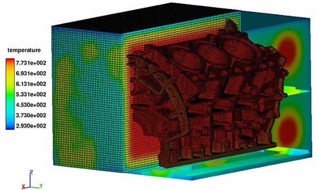
Figure 3: V6 엔진 블록의 온도 프로파일 단면도. 시뮬레이션 시작 7 초.

두번째 예제 시뮬레이션에서는 부분 커플링 모델을 사용하여 변형 가능한 강철 다이 내 금속 주물의 응력 개발을 보여 줍니다. 다이의 두 절반과 응고된 유체는 부분적으로 서로 결합되어 정상적인 응력과 마찰을 통해 상호 작용합니다. 시뮬레이션은 다이와 주물 부품의 열 응력 변화를 770,000 K의 solidus온도 바로 아래에서 298K의 주변 온도로 냉각하는 모습을 보여 줍니다. 주물 부분은 A380알루미늄 합금으로 구성되어 있고 다이 반쪽은 H-13강철로 구성되어 있습니다.

주조 부품과 주변 다이의 유한 요소 메시는 그림 3과 같이 3,665,533 요소와 3,862,378개 노드로 구성됩니다. 또한 각 다이의 절반에 대해 분리된 메쉬와 TSE고형화된 유체 영역도 나와 있습니다. 전면의 빨간 색 원은 서포트 피스톤 때문입니다(그림과 같이 표시되지 않음).

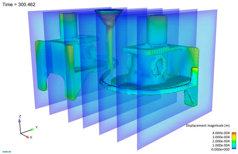
Thermal stress model — Figure 4 는 채워진 후 고압 다이 캐스팅 부품 300s의 주조물 온도와 변위 크기로 채색 된 강철 다이 조각을 결합한 이미지를 보여줍니다. 이 시뮬레이션에서, 다이는 응고하는 알루미늄에 연결되어 응력이 그들 사이에 전달됩니다. 변위 크기는 다이의 에지에서 0에서부터 주조에 인접한 0.1mm 이상까지 다양합니다.

금형과 응고된 유체 표면 사이의 경계면에서 발생하는 응력이 부분적으로 결합되어 제한된 수축을 확인할 수 있습니다. 그림 4는 시뮬레이션을 통해 주형 부분의 변형과 다이 부분의 절반의 변형을 보여 줍니다. 온도가 감소함에 따라 다이 캐스트와 주물이 서로 다른 속도로 수축하여 간섭 영역에 큰 응력이 발생하고 잠재적인 문제 영역이 나타납니다. 다이와 부품에서 결합된 응력을 계산하면 사용자가 각 구성 요소 내에서 발생하는 응력을 더 잘 예측하고 부품 품질을 개선하고 도구 수명을 연장하는 방법에 대한 통찰력을 제공할 수 있습니다.

Conclusion

다른 단단한 물체들의 상호 작용은 현대 디자인과 공학의 중요한 부분입니다. FSI구성 요소와 TSE고정 유체 영역 간의 새로운 결합 옵션이 FLOW-3D에 추가되어 오늘날의 엔지니어들이 정기적으로 접하는 복잡한 기하학적 구조를 평가하는 데 유용한 도구가 되었습니다.

다이 스프레이 냉각 / Die Spray Cooling

열 다이 사이클링 시뮬레이션에서 다이의 온도 분포를 정확하게 예측하려면 스프레이 냉각의 공간 변화를 모델링해야 합니다. 새로운 다이 스프레이 냉각 모델은 이러한 목적으로 개발되었으며 현재 FLOW-3D의 최신 버전에서 사용할 수 있습니다. 이 모델은 전체 다이 캐비티에 걸쳐 일정한 열 전달 계수를 가정하는 대신 각 스프레이의 냉각을 명시적으로 계산합니다. 다이 표면의 스프레이 영역은 스프레이 노즐의 움직임으로 인해 지속적으로 계산되고 업데이트됩니다. 또한 모델은 분무되는 유체의 차단을 고려하여 살수 각도와 다이 표면의 형태로 인해 냉각에 미치는 영향을 고려한다. 새로운 모델은 안정적이고 현실적인 입력 매개 변수를 사용하여 다이 표면에 정확한 온도 분포를 제공하여 엔지니어가 냉각 프로세스를 보다 효율적으로 설계하고 최적화하여 핫 스팟을 제거할 수 있도록 도와 줍니다.

스프레이 구역 계산 / Spray Area Computation

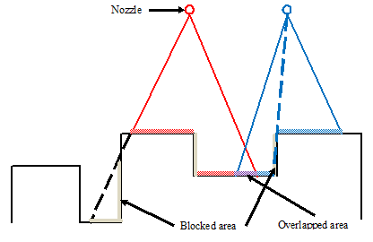
새 모델에서는 다이 표면의 형상과 분무 노즐 위치가 살수 냉각에 미치는 영향을 고려합니다. 아래 그림과 같이 다이 표면에 분사되는 일부 영역은 막히고 일부 영역은 2개 이상의 스프레이로 덮여 있습니다. 이러한 영역은 다양한 스프레이 냉각 효과를 구별하기 위해 광선 추적 알고리즘을 사용하여 계산하고 식별합니다. 스프레이 영역은 FlowSight^TM에서 시각화할 수 있으며, 스프레이 냉각을 통해 유닛 영역별로 제거된 총 분사 시간 및 총 열 등의 다른 특성도 확인할 수 있습니다.

열 전달 계수 결정 / Heat Transfer Coefficient Determination

스프레이 냉각 메커니즘은 복잡하며 스프레이 냉각 열전달 계수 (HTC)는 스프레이 모양, 냉각수 유량, 스프레이 압력, 금형 온도, 스프레이 각도 및 스프레이 거리와 같은 다양한 변수에 따라 달라집니다. 스프레이 냉각 HTC 계산을 단순화하기 위해, 모든 스프레이 표면 요소에 대해 HTC는 기본 요소 HTC에 종속 요소 (예 : 원추형 스프레이)를 곱하여 계산됩니다.

스프레이 냉각 메커니즘은 복잡하며, 스프레이 냉각 열 전달 계수(HTC)는 스프레이 형태, 냉각수 유량, 스프레이 압력, 금형 온도, 스프레이 각도, 스프레이 거리 등 다양한 변수에 따라 달라집니다. 스프레이 냉각 HTC의 계산을 단순화하기 위해 모든 스프레이 표면 요소에 대해 HTC는 기본 HTC에 원뿔형 스프레이의 경우와 같은 의존성 요인을 곱한 후 계산됩니다.

$\displaystyle HTC=HT{{C}_{0}}(T)\cdot {{f}_{d}}(d)\cdot {{f}_{b}}(\beta )\cdot {{f}_{e}}(\varepsilon )$

여기에서

₀HTCHTC는 노즐이 지정된 거리에서 몰드에 분사할 때 기본 스프레이 열 전달 계수입니다. 기준 열 전달 계수는 분무 콘의 특성, 살수 매체 및 살수 압력 등에 따라 달라지며, 주형 표면 온도의 함수입니다.
_dff는 거리 d종속 인자 함수이다.
_bff는 살수 각도β의존적 인자 함수이다.
_eff는(표면 법선과 살수 방향 사이의)살수 각도이며, Eu의존적 인자 함수이다.

스프레이 거리 d와 스프레이 각도 β 및 ε의 의미는 아래 그림과 같습니다

Spray distance and angle

기본 열 전달 계수 및 의존 계수 함수는 이론 또는 경험으로부터 유도 된 실험 측정으로부터 곡선 맞춤을 할 수 있습니다. 스프레이가 원추형이 아닌 경우 종속 요소가 다를 수 있습니다.

스프레이 노즐 정의 / Spray Nozzles Definition

분무 노즐은 뱅크로 분류된다. 동일한 뱅크의 노즐은 스프레이 콘 각도와 같은 특성을 가지고 있다. 또한, 동일한 살수 매체 온도와 동일한 그룹의 다이 구성 요소에 분사하고, 동일한 상태 제어 표를 공유하며, 동일한 열 전달 계수 기능을 가진다.

모든 스프레이 노즐 뱅크는 사실상 동일한 로봇 암에 장착됩니다. 로봇 암의 변환 및 회전 이동은 FLOW–3D 에서 지정할 수 있습니다. 모션 데이터가 외부 파일에 저장된 경우 외부 파일에서 가져오거나 연결할 수 있습니다. 스프레이 기계에 프로그래밍된 제어 데이터를 모델에 직접 사용할 수 있기 때문에 외부 파일을 가져오거나 연결할 수 있으면 입력이 상당히 간단해 집니다.

노즐 속성은 노즐 데이터베이스에서 직접 읽을 수 있습니다. 열 전달 계수 기능은 스프레이 콘 각도를 포함한 스프레이 콘 특성에 따라 달라지기 때문에 노즐 데이터베이스에 포함된 모든 노즐 특성의 일부입니다. 데이터베이스에 노즐이 정의되어 있지 않으면 그 속성을 직접 입력할 수 있습니다. 열 전달 계수 기능은 상수이거나 표로 정의할 수 있습니다. 다른 테이블 입력과 마찬가지로 데이터를 외부 파일에 연결할 수 있습니다. 동일한 노즐을 자주 사용하는 경우 재료 데이터베이스에 새 재료를 추가하는 것과 유사하게 해당 특성을 노즐 데이터베이스에 쉽게 추가할 수 있습니다.

각 노즐에 대해 스프레이 출처 및 엔드 좌표 또는 스프레이 방향을 정의해야 합니다. 노즐 위치가 미리 설계되어 있고 데이터를 사용할 수 있거나 노즐 수가 상대적으로 많을 경우 외부 파일에서 이 위치를 읽을 수 있습니다. 노즐 수가 적으면 위치를 대화식으로 선택하고 표 형식으로 입력할 수 있습니다.

Sample Results

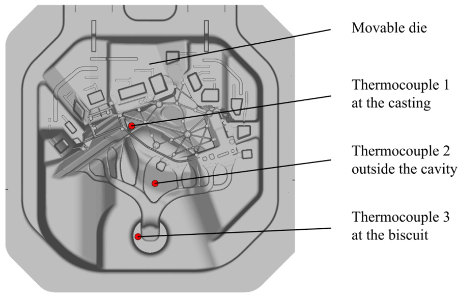
새로운 모델의 성능과 다이 스프레이 프로세스를 명시적으로 시뮬레이션하는 것의 중요성을 입증하기 위해 사례 연구가 수행되었습니다. 이는 큰 치수와 얇은 벽 두께를 가진 차량 구조 부품의 생산에 기초한다. 이젝터 다이의 다이 표면 안에 세개의 열전대가 배치됩니다. 위치는 다음 그림에 나와 있습니다. 첫번째 열전대는 주조 영역의 다이 표면에 배치됩니다. 두번째 열전대는 캐비티 밖에서 정의됩니다. 따라서 용해된 부분은 접촉하지 않지만 분사 과정 중에는 냉각되는 부분이 있습니다. 세번째 열전대는 비스킷에 있는데, 이것은 다이 내부의 핫 스폿입니다.

시뮬레이션은 5개의 사이클을 기반으로 하며, 각 사이클은 응고, 방출, 스프레이 냉각 및 주거라는 4개의 세그먼트로 정의됩니다. 전체 다이 캐비티에 걸쳐 일정한 열 전달 계수를 가정하는 암시적 다이 스프레이 냉각 시뮬레이션에서는 실제 공정 값을 사용할 수 없으므로 항상 스프레이의 평균 시간을 추정하기가 어렵습니다. 이 사례 연구에서는 열전대 1의 온도가 측정과 일치하도록 평균 시간을 추정하고 조정합니다. 반대로 각 스프레이 노즐의 냉각을 명시적으로 시뮬레이션하는 새로운 스프레이 냉각 모델의 경우, 실제 분사 프로세스에는 모든 시간 값이 포함되어 있어 시뮬레이션에 직접 전달될 수 있습니다. 이는 새로운 다이 스프레이 냉각 모델의 장점 중 하나입니다.

아래의 첫번째 애니메이션은 스프레이 냉각 중 다이 표면의 스프레이 영역을 보여 줍니다. 두번째 애니메이션은 다섯번째 주기에서 스프레이 냉각 중의 다이 표면 온도를 보여 줍니다. 글로벌 스프레이 및 핫 스팟 스프레이의 효과를 명확하게 확인할 수 있습니다.

Spray area during spray cooling. Simulation courtesy of Audi AG.

Die surface temperature at the fifth cycle of spray cooling. Simulation courtesy of Audi AG.

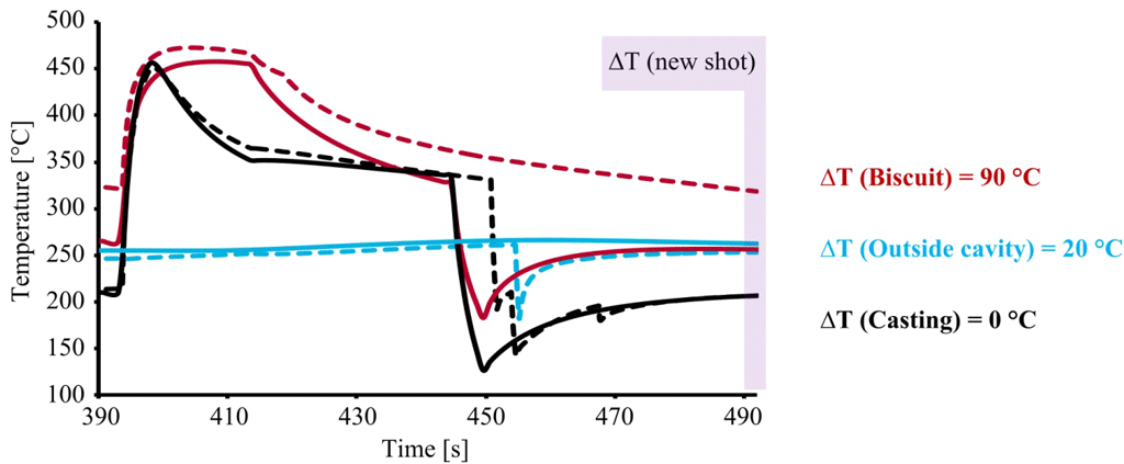
다섯번째 사이클 동안 세개의 열전대 온도가 다음 그림에 표시되어 있습니다. 실선은 암시적 모델의 결과를 나타내고 점선은 새로운 다이 스프레이 냉각 모델의 결과를 나타냅니다. 사이클이 끝날 때 세개의 열전대의 온도 차이도 표시됩니다. 암시적 모델에서 열전대 1의 온도를 일치시키기 위해 비스킷 영역이 지나치게 냉각되어 열전대 3에서 다이 온도의 90°C차이가 발생한다는 것을 알 수 있습니다. 이는 극적인 차이입니다. 다이 캐스터의 경우 비스킷의 온도는 다이 캐스팅 프로세스에서 매우 민감한 온도입니다. 사이클이 끝날 때 캐비티(열전대 2)외부의 온도 차이는 20°C입니다. 이러한 값은 실제 공정에서 우수한 품질의 주물이 생산되거나 사출 중에 다이에 응고되는지 여부를 결정합니다. 다이 스프레이 냉각 프로세스의 명확한 시뮬레이션은 정확한 다이 온도 분포를 예측하는 데 매우 중요합니다.

Temperatures thermocouples - die spray cooling model

Conclusions

새로운 다이 스프레이 냉각 모델은 몰드 표면 형태의 영향과 스프레이 노즐의 위치 및 움직임을 고려하여 FLOW-3D 사용자에게 다이 준비의 모든 측면을 모델링 할 수 있는 능력을 제공합니다. 또한 열 다이 사이클 시뮬레이션을 위한 신뢰할 수 있고 사실적인 입력 파라미터를 사용하여 다이 표면의 정확한 온도 분포를 정확하게 예측할 수 있습니다. 이를 통해 금속 주물 엔지니어는 다이의 내부 냉각 구조와 스프레이 냉각 매개 변수를 보다 효율적으로 설계하고 평가할 수 있습니다.

References

Müller, et al., A die spray cooling model for thermal die cycling simulations, Transactions of NADCA 2015 Die Casting Congress & Exposition, Indianapolis, T15-101, 2015

실험 (위) 및 FLOW-3D 결과 (아래)의 비교. x 축은 거리입니다 (실험 사례에 대해 정규화 됨). y 축은 소스 농도 (실험 사례의 경우 형광 강도)입니다.

Microfluidic palette – A gradient generator / 미소유동 팔레트 – 그라디언트 생성기

Microfluidic 팔레트 – 그라디언트 생성기

Microfluidics 모델링 , 그래디언트 생성 장치 시뮬레이션 및 검증 작업을 계속하는 것은 Flow Science의 최신 연구분야입니다. 확산 기반 그라디언트는 많은 복잡한 생물학적 과정에서 없어서는 안될 부분입니다. 한 예로 세포가 화학적 구배를 따라 이동하는 화학 주성 (chemotaxis )으로 인한 상처의 치료 방법입니다. 지난 몇 년 동안 확산 구배를 설정하고 연구하기 위한 다양한 접근법이 등장했지만 모두 문제 해결에 어려움을 겪고 있습니다.

Atencia 등은 이전 접근법의 알려진 문제점을 극복하기 위해 혁신적인 미세 유체 구배 생성기 (마이크로 유체 팔레트)를 제안했습니다.

이전 접근법 및 관련 문제

확산 그라디언트를 설정하는 세 가지 주요 접근법으로 층류, 멤브레인 및 하이드로 겔 및 자유 확산 방법이 있으며 각각의 특징이 았습니다. 그러나, 언급한 것처럼 문제를 해결하는데 동반되는 어려움이 있습니다.
microfluidic 장치에서 그라디언트를 연구하고 확립하기 위한 표준 접근법은 층류의 사용을 포함합니다. 이 접근법은 매우 간단하지만 대류로 인해 전단 응력이 발생합니다. 전단 응력은 세포 반응을 변화시킬 수 있습니다. 예를 들어, 바이어스 된 세포 이동 및 비대칭 대량 수송이 발생할 수있습니다.

보다 최근의 개발은 강성 멤브레인 및 하이드로 겔을 사용하는 것을 포함하여 확산 구배를 설정하여 대류 흐름을 피하는 것입니다. 그러나 막과 겔은 확산 속도를 감소시켜 그라데이션의 일시적인 현상에 영향을줍니다.

마지막으로, 2 개의 유체 플러그를 접촉시켜 자유로운 확산을 가능하게 하는 접근법이 개발되었습니다. 그러나 이 접근 방식은 1-D 흐름에만 국한됩니다. 또한, 일단 그래디언트가 설정되면, 확산류 구배를 수정하기 위해 대류 흐름을 사용해야 하며, 이는 층류 유동에서 전단 응력 발생의 초기 문제로 되돌아갑니다.

여기에서는 Atencia 등이 제안한 확산성 구배 생성에 대한 새로운 접근법의 원리에 대해 논의하고 FLOW-3D 시뮬레이션 결과를 제시합니다.

Microfluidic 팔레트

미세 유체 팔레트 뒤에있는 원리는 멤브레인이나 젤을 사용하지 않고 확산으로부터 대류 흐름을 분리하여 다음과 같은 이점을 제공합니다.

전단 응력없이 재료 (셀 또는 용해성 물질)의 전달
서로 다른 공간 위치를 갖는 중첩 그라데이션 생성
그라데이션에 대한 동적 제어

Atencia 등이 제안한 미세 유체 팔레트의 디자인은 위에 나와 있습니다. 1-D의 경우, 대류 장치 1의 질량 균형은 입구 1과 출구 1의 유속을 일치 시키면 확산을 통해 전달을 허용하면서 주 마이크로 채널을 통한 흐름을 방지합니다. 대류 장치 1은 완벽한 소스 역할을 합니다. 2 차원의 경우는 2 차원 이상의 대류 단위가있는 1 차원의 경우를 단순히 확장한 것입니다.

FLOW-3D 시뮬레이션

아래의 1 차원 마이크로 유체 팔레트 애니메이션에서 주 중앙 마이크로 채널로부터의 대류 세포의 깨끗한 분리는 플롯 된 유선을 통해 볼 수 있습니다. 유선형은 모두 대류 단위에만 제한되며 단일 채널도 마이크로 채널로 누출되지 않아 대류와 확산의 탁월한 분리를 나타냅니다. 소스 농도의 진화는 플롯에서 볼 수 있습니다. 플롯은 애니메이션이 끝날 때까지 일정하게 보입니다.

1 차원 마이크로 유체 팔레트의 FLOW-3D 시뮬레이션 결과

2D 마이크로 유체 팔레트는 생성 된 그라데이션에 대한 시공간 제어를 보여줍니다. 소스와 싱크는 각속도로 회전합니다. 또한 매 초마다 활성 액세스 포트가 비활성화되고 다음 포트가 켜집니다. 챔버 내부의 확산 상태를 확인하기 위해 3 개의 라인 프로브가 시뮬레이션에 배치됩니다 (아래 시뮬레이션의 오른쪽 하단 창에서 각각 빨간색, 파란색 및 검은 색으로 표시됨).

2D 3D 마이크로 유체 팔레트의 FLOW-3D 시뮬레이션 결과.

실험 결과와의 비교

FLOW-3D 결과는 챔버 내부의 농도 변화 측면에서 실험 결과와 잘 일치합니다. 아래 이미지는 실험 결과와 시뮬레이션 결과 모두에 대한 시간 스냅 샷을 보여줍니다. 실험 결과가 정규화되었습니다. 또한 실험은 형광 강도를 사용하여 소스의 농도를 나타냅니다. 시뮬레이션에서 FlowSight 의 라인 프로브는 3 개의 액세스 포트 사이의 농도를 연구하는 데 사용됩니다.

References

Atencia J, Morrow J, Locascio L.E., The microfluidic palette: A diffusive gradient generator with spatio-temporal control, The Royal Society of Chemistry 2009

응고 및 수축 / Solidification & Shrinkage

응고 및 수축

FLOW-3D에서 금속 합금의 응고 모델링은 잠열의 방출뿐만 아니라 응고 물질의 전이 단계를 추가 포함합니다. 응고 모델은 다양한 주조 공정을 모델링 할 때 사용할 수 있습니다.

Modeling the two-phase solid/liquid flow of metal during solidification

고체화되는 동안 금속의 2 상 고체/액체 흐름을 모델링하는 것은 흐릿한 영역을 3 개의 영역으로 분할함으로써 접근합니다. 응고의 초기 단계에서, 형성되는 고체 결정은 서로 분리 된 것으로 가정됩니다. 따라서, 고체 / 액체 혼합물은 하나의 유체로서 움직입니다. 그러한 유체의 유효 점도는 순수한 액체의 점도보다 높고 고체 분율의 함수로 계산됩니다.

고형분이 일관성 지점에 도달 할 때, 응고된 결정을 따라서 이동하지 않고, 주형 벽에 부착되는 강성의 골격을 형성합니다. 유동은 다공성 미디어가 되고, 이동 유체에 다르시 형 항력을 적용하여 모델링됩니다.
마지막으로, 고체 분율이 임계 값을 초과하면, 응고된 금속은 액체 금속이 더 이상 흐르지 못하는 고밀도 구조를 형성합니다. 이것은 무한히 큰 항력을 적용하여 모델링됩니다. 이 후에도 응고가 계속 되더라도 금속은 효과적으로 동결 된 것으로 간주됩니다.

Mold 충진
응고 모델은 금형 충진 및 금형 내부의 금속 냉각에 사용될 수 있습니다. FLOW-3D 의 다양한 물리적 모델은 이 기본 응고 방식에 연결할 수 있습니다.

binary alloy segregation model 은 응고 금속의 열 및 solutal 부력 구동 흐름을 형성하여 거시 분리 패턴을 예측합니다.
응고되는 동안 부피 수축으로 인한 매크로 및 미세 다공성의 형성도 기술 될 수있습니다.
결함 추적 및 공기 함몰 모델과 함께 다공성 모델은 최종 부품의 품질을 평가하는 데 도움이됩니다.
특별 기준 기능을 사용하여 1 차 및 2 차 수상 돌기 암 간격의 변화를 예측할 수 있습니다.
탄성 응력 모델은 냉각 부품의 응력 및 변형을 계산합니다.
드리프트 플럭스 모델을 사용하면 반 고체 금속 주조 공정 중에 액체 및 고체상 분리를 설명 할 수 있습니다.

암시적 열전달 모델 및 제로 속도 필드 모델과 같은, 보다 효율적인 계산을 위해 특수 수치 모델도 사용할 수 있습니다. 후자는 금속 유동이 응고 역학에 미치는 영향을 무시할 수 있을 때 유용합니다. 이는 채우기가 완료된 후 종종 발생합니다.

퇴적, 세굴(쇄굴) / Sediment Scour

퇴적-세굴(쇄굴) / Sediment Scour

유체 역학과 완벽하게 연계된 FLOW-3D 의 sediment scour model은 침전물 수송, 부유물 운반, 인입 및 퇴적을 포함하여 비 점착성 토양의 모든 퇴적물 이동 과정을 모의 실험합니다 (Wei 등, 2014). 입자 크기, 질량 밀도 및 임계 전단 응력과 같은 다른 성질을 갖는 다중 퇴적물 종을 허용합니다. 예를 들어, 중간 모래, 거친 모래 및 자갈은 시뮬레이션에서 세 가지 종으로 분류 할 수 있습니다. 이 모델은 3D 흐름과 2D 천수(shallow water) 흐름에 모두 적용됩니다.

모델에서, 퇴적물의 충진 층은 퇴적물 종의 상이한 조합을 갖는 다수의 하위 구성 요소로 구성 될 수있는 하나의 기하학적 구성 요소에 의해 정의됩니다. 충전된 베드는 면적 및 부피 분율을 사용하는 FAVOR^TM 기술에 의해 기술된다. 베드 인터페이스를 포함하는 메쉬 셀에서 인터페이스의 위치, 방향 및 면적이 계산되어 베드 전단 응력, 임계 실드 매개 변수, 침식 속도 및 베드로의 전송 속도를 결정합니다. 3 차원 난류 유동에서의 전단 응력은 매체 입자 크기 50 에 비례하는 층 표면 거칠기를 고려한 표준 벽 함수를 사용하여 평가됩니다. 2D 천수(shallow water)의 경우, 층 전단 응력 계산은 항력 계수가 사용자 정의이거나 수심과 층 표면 거칠기를 사용하여 국부적으로 계산 된 2 차 법칙을 따릅니다.

그림 1. t = 8 분에서의 유량
이 모델은 Meyer-Peter와 Muller (1948)의 방정식을 사용하여 베드 인터페이스를 포함하는 각 메쉬 셀에서의 베드로드 이송을 계산합니다. 서브 메쉬 (submesh) 방법은 메쉬 셀에서 이웃에있는 각 메쉬 셀로 이동하는 입자의 양을 결정하는 데 사용됩니다. 부유 퇴적물 농도는 퇴적물 수송 방정식을 풀음으로써 얻어집니다. 침식의 계산은 침전물 유입 및 침전을 동시에 고려합니다. entrainment에서 입자의 리프팅 속도는 Winterwerp et al. (1992). 퇴적시의 침강 속도는 3D 유동에 대한 퇴적물의 표류 속도와 같지만 얕은 수류에 대해서는 현존 방정식을 사용하여 계산됩니다 (Soulsby, 1997). 드리프트 플럭스 이론 (Breitour and Hirt, 2009)은 입자의 드리프트 속도를 계산하는 데 사용됩니다.

그림 2. t = 8 분의 구멍 채취
이 페이지의 예는 3 개의 원통형 교각을 중심으로 한, 맑은 물 정화에 대한 시뮬레이션입니다. 교각의 지름은 1.5m이며, 교각은 2m 간격으로 나란히 배치되어 있습니다. 다가오는 유량은 실린더와 정렬되며 2m/s의 속도를가집니다. 베드 재료는 모래 (직경 5mm), 자갈 (10mm) 및 거친 자갈 (20mm) 인 세 가지 퇴적물 종으로 구성됩니다. 그림 1, 2 및 3은 8 분간 실린더 주변의 흐름, 채취 구멍 및 채취 깊이 분포를 보여줍니다.

그림 3. t = 8min에서의 정련 깊이 (양수 값) 및 침전 높이 (양수 값)
이 모델에 대한 더 자세한 정보는 침전물 퇴적에 관한 Flow Science Report를 다운로드하십시오.

점탄성 흐름 / Viscoelastic Flow

FLOW-3D 는 국부 변형률 및 변형률 속도에 따라 액체와 고체처럼 거동하는 재료의 거동을 예측하는 점탄성 유동 모델을 포함합니다. 점탄성 물질은 고분자 용액, 용융물 및 고충진 입자의 현탁액을 포함합니다. Elasto-viscoplastic 소재는 항복 응력 한도까지 안정된 거동을 나타내며 그 이상의 재료는 액체와 같은 거동을 나타냅니다.

FLOW-3D에 포함 된 점탄성 모델에는 Oldroyd-B 모델과 Giesekus 모델이 있습니다. 추가 모델은 사용자 정의를 통해 구현 될 수 있습니다.
재료에 관계없이 탄성 응력은 하나의 시간 간격에서 점차적으로 계산되어 장시간 동안 큰 변형을 시뮬레이션 할 수 있습니다.

스퍼 기어의 사출 성형 / Injection molding of a spur gear

한 가지 예가 폴리에틸렌 용융물의 사출 성형입니다. 위의 애니메이션은 스퍼 기어의 사출 성형을 보여줍니다. 동일한 부품은 동일한 점성 속성을 갖는 다른 (허구의) 소재로 채워지지만 탄성 속성은 없습니다. 탄성 응력의 효과는 유체가 기어의 바깥 쪽 테두리에 도달 할 때 명확합니다. 여기서는 점탄성 물질의 압출 공정에서 볼 수 있듯이 쐐기에서 발생하는 탄성 응력이 대칭적인 “흘러 내림”에서 거의 수평 운동으로 흐름을 변경합니다.

난류 / Turbulence

FLOW-3D 는 완전 3 차원 유동, 2 차원 깊이 평균 (천수(shallow water)) 흐름 및 3 차원/2 차원 깊이 혼합 평균 흐름을 위한 포괄적인 난류 모델링 제품군을 제공합니다.

그림1. 부두 하류에서의 와류 검출을위한 Q- 기준의 3D지도

FLOW-3D 에는 8 가지 난기류 옵션이 있습니다.

Prandtl 혼합 길이 모델은 3 차원 난류 효과를 설명하기 위한 가장 초기의 시도 중 하나입니다. 가장 복잡한 모델이 아니며 더 이상 널리 사용되지 않습니다. FLOW-3D 는 주로 학술 연구에서의 유용성을 포함합니다.
소위 1 방정식 모델은 난기류를 나타내는 초기 노력이기도 합니다. 시간 평균 난류 운동 에너지 k를 계산하고 모든 위치에서 알려진 난류 혼합 길이 L_T 가 필요합니다. L_T 는 일반적으로 미리 알려지지 않기 때문에, one-equation 모델은 복잡한 유량을 모델링하는 데 적합하지 않습니다.
표준 k-ε 모델 (Harlow & Nakayama 1967)은 난류 운동 에너지 k와 소산 속도 ε를 계산하고 난류 혼합 길이 L_T를 동적으로 찾는 2 방정식 모델입니다. 이것은 업계 표준이며 광범위한 흐름을 표현하는데 유용하다는 것이 발견되었습니다 (Rodi 1980).
재 정규화 그룹 (RNG) k-ε 모델 (Yakhot & Orszag 1986, Yakhot & Smith 1992)은 2 방정식 k-ε 모델의 보다 견고한 버전이며, 대부분의 산업에서의 문제에 권장됩니다. 표준 k-ε 모델의 기능을 확장하여 과도기 난류, 곡선 흐름, 벽 열 전달 및 물질 전달의 더 나은 적용 범위를 제공합니다.
k-ω 2 방정식 모델 (Wilcox 1988, 1998, 2008)은 두 번째 변수를 난류 소산 ε이 아니라 ω ≡ ε / k로 정의한다 (Kolmogorov 1942). Wilcox는 1988 년부터 k-ω 2 방정식 모델을 개선했으며 1998 년에는 자유 전단 유동에 대한 모델의 정확성을 크게 개선 한 새로운 계수를 도입했습니다. FLOW-3D 의 k-ω 2 방정식 모델은 제트, 후류 및 플럼을 퍼 뜨리는 것과 같은 유선형 압력 구배를 갖는 자유 전단 흐름을 모델링하는 데 적합합니다.
LES 모델은 평균 난류 운동 에너지를 나타내기 위해 스칼라를 사용하지 않고 대부분의 난류 변동을 직접 해결합니다. 그것은 2 방정식 모델보다 훨씬 더 미세한 메쉬 해상도를 필요로하며 난기류에 대한 보다 광범위한 통계를 제공합니다.
2-D 심도 평균 얕은물 난류 모델은 대수적인 완전 난류 속도를 가정합니다. 첫 번째 옵션은 일정한 항력 계수 CD를 가정하며, 이는 공간적으로 변화 할 수 있습니다.
두 번째 2-D 심도 평균 천수(shallow water) 난류 모델은 항력 계수 CD 를 유체 깊이와 공간적으로 가변되는 표면 거칠기의 동적 함수로 만듭니다.

완전한 3-D 테스트를 통해 LES 모델 출력을 시간 평균화하면 2 방정식 Reynolds REN (Reynolds Averaged Navier-Stokes) 모델 (표준 k-ε, RNG k-ε 및 k- ω).

아래의 물고기 통로 비디오에 나와 있습니다.

난류 시뮬레이션 – 모델 비교 / Turbulence Simulations – A Model Comparison

첫 번째 비디오에서는 FLOW-3D 의 LES (Large-Eddy Simulation) 난류 모델을 사용하여 어류 통과를 시뮬레이션하여 속도 변동의 크기를 분석합니다. 두 번째 비디오는 동일한 시뮬레이션의 시간 평균 결과를 보여줍니다. 여기에서 간단한 사용자 정의는 시간 평균 LES가 레이놀즈 평균 Navier-Stokes (RANS) 난류 모델 결과와 매우 유사하다는 것을 보여줍니다. 세 번째 비디오는 RNG (Renormalized Group) k-ε 난류 모델을 사용하여 시연하기 위해 동일한 시뮬레이션을 사용합니다. RNG k-ε 모델은 대부분의 레이놀즈 평균 Navier-Stokes (RANS) 난류 모델과 마찬가지로 속도 변동을 등방성 스칼라 값으로 처리하여 시간에 따른 속도 변동을 감쇠시킵니다. 결과는 두 번째 비디오에서 볼 수 있듯이 직접 LES 결과를 시간 평균하여 찾은 결과와 유사합니다.

참고 문헌

Driver, DM and Seegmiller, HL, 1985, AIAA Journal (23), 163-171의 다양한 채널 유동에서 재 부착하는 난류 전단 층의 특징 .
Harlow, FH and Nakayama, PI, 1967, 난류 수송 방정식 , 유체 역학 (10), 2323-2332.
Harlow, FH 및 Nakayama, PI, 1968, 난기류 에너지 감쇠율의 전송 , Los Alamos Scienti fi c 실험실 보고서 LA-3854.
Kolmogorov, AN, 1942, 비압축성 유체에서의 난류 운동 방정식 , Izvestia Academy of Sciences, 소련; Physics (6), 56-58.
Pope, S. B, 2000, Turbulent Flows , Cambridge University Press.
Rodi, W., 1980, 난류 모델과 유압 장치의 적용 : 최첨단 검토 , 국제 유압 연구 협회 (IAHR), 델프트, 네덜란드.
Saffman, PG, 1970, Inhomogeneous Turbulent Flow의 모델 , Royal Society London A (317), 417-433의 절차.
Speziale, CG, Abid, R., and Anderson, EC, 1992, AIAA 저널 (30), 324-331, 벽 근처 난류에 대한 2 방정식 모델의 중요성 평가.
Wilcox, DC, 1988, AIAA Journal (26), 1299-1310의 진보 된 난류 모델에 대한 스케일 결정 방정식의 재평가.
Wilcox, DC, 1998, CFD의 난류 모델링 , DCW Industries, Inc., 제 2 판.
Wilcox, DC, 2008, k-omega 난류 모델의 공식화 , AIAA Journal (46), 2823-2838.
Yakhot, V. and Orszag, SA, 1986, 난류의 재 정규화 그룹 분석 I. 기본 이론 , Journal of Scientific Computing (1), 3-51.
Yakhot, V. 및 Smith, LM, 1992, 재 정규화 그룹, 난류 모델의 전자 확장 및 유도 , Journal of Scientific Computing (7), 35-61.

표면 장력 / Surface Tension

FLOW-3D에 추가 된 최초의 물리 모델 중 하나는 표면 장력이었습니다.

이 모델은 잉크젯, 무중력 환경에서의 액체 연료 거동 및 다양한 MEMS (마이크로 전자 기계 시스템) 장치와 같이 다양한 종류의 응용 분야에서 수년 동안 널리 사용되어 왔습니다. 이 후에 모델의 개선 및 확장에 대한 많은 사용자 요청이 처리되었습니다.
표면 장력에 대해 보다 나은 성능개선을 위해 FLOW-3D 버전 11에 대한 새로운 모델이 개발되었습니다. 이 모델은 계산된 모든 표면 장력의 정확성과 임의 형상의 솔리드 표면을 잡아 당기는 접착력의 정확성을 향상시킵니다. 또한 이 새로운 모델은 다공성 물질의 모세관 압력과 비 균일한 표면 장력으로 인한 접선 표면 장력을 가지고 있습니다.

새로운 모델의 예는 무중력에 포함된 원형 벽을 적시는 단순한 문제입니다.

그림 1은 실린더와 접촉각이 0 도인 물로 채워진 0.25m 직경의 실린더 75 %의 경우를 보여줍니다. 버블은 10 초 전에 벽에서 깨끗하게 분리되어 탱크를 가로 질러 움직입니다. 비 구형은 기포 표면에서 모세관 파가 전파되기 때문입니다.

그림 1. 0.0, 2.5, 5.0 및 10.0 초에 무중력에서 접촉 각이 0 인 실린더 표면의 유체 (적색) 습윤 표면.

다른 예가 그림5에 도시되어 있습니다. 2에서 서로 다른 밀도의 2 개의 초기 구형 방울이 (플롯의 색으로 표시됨) 단단한 벽을 향해 아래로 이동합니다. 플롯의 시간은 0.0, 0.01, 0.02 및 0.03 초입니다. 방울은 직경이 0.0017m, 밀도가 다르지만 표면 장력 계수는 1.872 뉴턴 / m입니다.

그림 2. 접시쪽으로 움직이는 구형의 물방울. 새로운 표면 장력 모델로 시뮬레이션. 색상은 밀도를 나타냅니다.

표면 장력 모델에 대해 자세히 알아보십시오.

Download the Flow Science Report on Surface Tension

Download Surface Tension Validation – Simple Test Problems

소금 용해 / Salt Dissolution

액체의 소금 용해는 식품 가공, 의료 어플리케이션에 이르기까지 많은 CFD 어플리케이션과 관련됩니다. 이 기사는 유체에 소금을 녹이고 소금물에서 용질을 추적하는 전산 모델의 예비 결과를 설명합니다. 제안된 모델은 소금과 유체 사이의 계면에서의 물질 전달, 고체 염의 체적과 형태의 변화, 유체에서 용해 된 염의 확산과 대류, 점도 및 표면 장력, 그리고 마지막으로 유체 밀도의 변화와 같은 기본적인 물리적 현상을 설명합니다.

소금 모델링에 대한 수치적 접근

액체 내의 용해된 염의 양은 그의 질량 농도 C로 표시 된다. 액체 / 고체 염분 경계에서의 소금의 질량 유량 Q 는 Q = k ( C SAT – C )로 정의되며, 여기서 k는 일정 질량 전달 계수이고 C_SAT 는 소금의 포화 농도이다. 유체 혼합물 밀도는 소금 농도의 선형 함수로 가정됩니다. 체적은 또한 농도에 따라 다를 수 있습니다. 예를 들어 상온에서 포화 된 해수 (염수)의 밀도는 담수의 밀도보다 약 26% 크며 부피는 13% 증가합니다.

일단 용해 된 소금이 계산 그리드의 제어량에 분배되면, 확산 및 대류가 혼합물 내에서 염을 인계하고 재분배합니다. 유동 영역에서 고체 염의 존재와 유체에 용해된 용적 및 형태의 변화를 설명하기 위해 GMO (General Moving Object) 모델의 변형이 개발되었습니다. 솔리드 솔트를 나타내는 지오메트리 구성 요소는 특수 유형의 구성 요소로 지정됩니다. 이동하는 대신 모양과 볼륨이 변경됩니다. 면적 및 부피 분율은 고체 염의 점진적인 용해를 반영하여 매 시간 단계마다 다시 계산됩니다.

시험 예 : 약물 용해

모델은 피부 패치에서 땀에 의해 약의 고체 결정의 용해를 근사하는 테스트를 사용하여 설명됩니다. 도메인의 3 차원 기하학은 Fig. 1. 도메인의 크기는 4.5 mm x 2 mm x 0.8 mm입니다. 동일한 원통형 장애물 ( “핀”)의 규칙적인 패턴이 정의되며, 각 핀의 직경은 0.5 mm이고 높이는 0.65 mm입니다.

그림 1. 테스트 문제에 대한 계산 도메인의 개략도. 화살표는 입구 경계를 나타냅니다. 초기 고체 염분 블록은 녹색 성분으로 표시됩니다.
염분 용해 속도는 도메인이 모세관 력에 의해 유체에 의해 처음으로 채워지는 속도보다 훨씬 작기 때문에, 문제는도 1의 화살표로 나타낸 방향을 따라 고정 된 유속으로 한정된 유동으로 모델링된다. 그 결과를도 1에 나타낸다. 2.

그림 2. t = 48 초 (오른쪽) 유체의 농도에 의해 색깔 소금 블록의 모양과 바닥 경계 (왼쪽)을 따라 수평 단면의 유체에 용해 소금의 분포.

5,000 dynes의 압력 차이는 0.25cm/sec의 평균 유속을 산출합니다. 평균 유속은 유속과 함께 유속이 증가함에 따라 소금이 용해됨에 따라 점진적으로 증가합니다. 용해된 염분이 흐름에 의해 씻겨지기 때문에 고체 염분의 상향 류 측은 하류 측보다 빨리 용해됩니다. 하류 쪽의 혼합물은 더 포화되어 이 지역의 용해 과정을 늦춘다. 이 특별한 시험의 또 다른 관찰은 대류와 비교하여 유체에서 염의 확산이 작다는 것입니다.
새로운 소금 용해 모델은 FLOW-3D에 유용한 추가 기능 입니다. 첫 번째 원칙에 입각하여 이 모델은 소금 채굴에서부터 천연 가스 저장을 위한 지하 공동 생성, 약물 전달, 금속 합금에 이르기까지 다양한 상황에서 사용될 수 있습니다. 움직이는 물체 모델을 멋지게 확장 한 것으로, 시간에 따라 달라지는 면적 및 부피 분율을 사용하여 움직이는 단색 경계를 설명합니다.

다상 유동 / Multiphase Flows

다단계 흐름(다상 유동) / Multiphase Flows

극저온 액체 / 가스 조합 및 제 2 비응 축성 가스 성분을 함유하는 탱크

FLOW-3D 의 상 변화 모델은 액체 / 기체 계면에서의 기화 및 응축을 시뮬레이션합니다. 그것은 주위 액체에 증기 기포의 형성과 상호 작용을 예측합니다. 기포는 핵 생성을하고 액체 운동에 역동적으로 반응하며 주변 환경의 온도와 압력에 따라 성장하거나 줄어들 수 있습니다.
FLOW-3D 의 기존 상 변화 모델은 증기 기포와 주변 액체의 형성과 상호 작용을 예측하는 강력한 도구입니다. 기포는 액체 운동에 동적으로 반응 할 수 있으며 주위 환경의 온도와 압력에 따라 성장하거나 줄어들 수 있습니다 . 그러나, 증기와 함께 존재할 수 있는 응축되지 않는 가스의 효과를 기포 또는 다른 증기 공간 내부에 포함시키는 것은 아직 가능하지 않습니다.

예를 들어 수증기와 공기가 모두 포함 된 기포가 증기보다 더 낮은 온도 또는 더 낮은 조건에서 존재할 수있는 공기 / 물 / 증기 시스템의 역학에서 중요 할 수 있습니다. FLOW-3D 는 사용자가 비 응축 가스를 모델링 할 수있게 하여이 제한을 없앱니다.

하이라이트

사용자는 가스 상수, 열용량 및 증발 데이터의 열을 제공하고 관련 초기 및 경계 조건 데이터 만 지정하면됩니다.
기체 / 액체 계면이 존재하는 곳에서는 액체의 증발과 증기의 응축이 자동으로 계산됩니다.
사용자는 응축되지 않는 가스 및 증기의 부피 분율을 그래픽으로 추적 할 수 있습니다.

모델 기본 사항

이 모델은 날카로운 인터페이스 추적과 함께 FLOW-3D 의 압축성 2-유체 흐름 옵션과 함께 사용해야합니다. 비 응축 가스의 국부적인 농도를 추적하는 새로운 양은 모델이 가스 / 증기상 내에서 가스의 효과를 예측할 수있게 합니다. 가스 상수 및 열용량에 대한 조정은 압력 – 밀도 관계를 변경시킵니다. 그러므로 기체 / 증기 혼합물에서 응축 가능한 상 (condensable phase)의 증기압의 계산은 증기의 체적 분율에 국소 절대 압력을 곱한 값입니다.

따라서 모델의 기초는 물질 전달률의 계산입니다 :

실험 및 시뮬레이션 데이터를 사용한 샘플 결과

극저온 탱크 내의 압력 도표 : 테스트 데이터 (빨간색)와 FLOW-3D 모델 (파란색)의 비교. 압력은 탱크 벽을 통한 점진적인 가열로 인해 상승하고 차가운 질소 스프레이의 도입으로 인해 급격히 감소합니다.
극저온 액체 / 가스 조합 및 제 2 비응축성 가스 성분을 함유하는 탱크의 이러한 예에서, 탱크의 벽은 특정 탱크 압력에 도달 할 때까지 서서히 가열되고,이 시점에서 차가운 액체 스프레이가 급속하게 도입되어 온도를 낮추는 탱크를 감압하십시오. 이 프로세스는 주기적입니다.

이 모델을 기반으로하는 연구는 미국 항공 우주 학회 (American Institute of Astronautics) 회의에서 발표 되었습니다. 이 연구에는 실제 테스트 데이터와 액화 가스를 포함하는 극저온 탱크의 계산 시뮬레이션을 비 응축 가스 (일반적으로 헬륨)와 비교하여 비교했습니다. 왼쪽의 플롯은 시간의 함수로서 질소 증기 및 헬륨 가스를 함유 한 가스 공간을 갖는 액체 질소를 함유하는 탱크의 증기 영역 내의 압력을 도시합니다. 예를 들어, 탱크의 벽에서 탱크 압력이 25 psi에 도달 할 때까지 서서히 가열합니다. 이 시점에서 차가운 액체 질소 스프레이가 도입되어 탱크를 급냉(따라서 감압) 합니다. 그런 다음 이 과정이 반복됩니다. 시뮬레이션 데이터는 실제 테스트 데이터와 잘 일치하였습니다. 오류는 일반적으로 ~ 10 % 정도입니다. FLOW-3D 모델과 테스트 데이터 간의 오차는 부분적으로 열 전달 계수를 측정하기 어렵기 때문에 모델에서의 열전달율이 일정하다고 가정하고 액체 스프레이를 탱크는 일정한 온도로 유지됩니다.

움직이는 물체 / Moving Objects

FLOW-3D 시뮬레이션에서 일반적인 움직이는 물체 (GMO)는 사용자가 규정하거나 유체 흐름과 동적으로 결합되는 모든 종류의 모션을 가진 강체입니다. 고정된 축 / 포인트와 같은 6 자유도 또는 모션 구속 조건을 가질 수 있습니다. 규정된 힘과 토크는 결합된 동작 하에서 GMO에 적용될 수 있습니다. GMO 모델은 충돌 및 연속 접촉을 포함하여 강체 상호 작용뿐만 아니라 독립적인 동작 유형에서 여러 개의 강체를 허용합니다. 이 모델은 견고하고 효율적이며 강력하고 상업용 전산 유체 역학 소프트웨어에서 FLOW-3D가 유일합니다.

FLOW-3D 자동차 차동 부분의 3D 시뮬레이션

모델링 기능

6 개의 DOF를 소유 할 수있는 최대 500 개의 움직이는 물체를 허용하거나 고정된 축 또는 고정된 점을 중심으로 회전 할 수 있습니다. 다른 모션 제약 패턴도 가능합니다.
물체는 유체 흐름과 완벽하게 결합되거나 사용자가 모션을 처리할 수 있습니다.
물체는 밀도로 특징 지어지는 여러 가지 재료로 만들 수 있습니다.
객체의 기하학 및 동작의 복잡성에 대한 제한이 없습니다.
지정된 시간에 따른 힘과 토크를 대상에 적용 할 수 있습니다.
모델 충돌 및 움직이는 물체와 움직이지 않는 물체 사이의 지속적인 접촉
스프링과 로프는 물체에 닿을 수 있습니다.
개체에서 다공성 허용
열전도 및 대류가 허용됩니다.
유압식, 중력 식, 비 관성식, 스프링 식, 사용자 정의 제어력 및 토크는 결합 된 모션이있는 물체에 대해 고려됩니다.
시각 및 수치 출력을 포함한 완벽한 후 처리 기능

움직이는 물체 시뮬레이션

FLOW-3D 고객은 처음 사용하는 방법보다 더욱 효율적으로 움직이는 물체 모델의 적용을 사용했습니다. waterwheels에서 shot sleeve, 에너지 디바이스 파동에 이르기까지 우리는 복잡한 메쉬 및 집중적인 컴퓨팅 리소스에 의존하지 않고도 엔지니어링 문제를 해결하는데 모델을 사용하는 방법에 깊은 인상을 받았습니다. 이 모델을 사용하는 진지하고 상상력이 좋은 예를 모두 검토하려면 YouTube 재생 목록 을 방문하십시오.

계류 라인 / Mooring Lines

계류 라인 Mooring Lines

현재 버전의 FLOW-3D 는 여러 움직이는 물체를 탄성 로프를 통해 다른 움직이는 물체 또는 고정 된 장소에 연결할 수 있습니다.

로프는 무겁고 늘릴 때 항상 직선으로 간주됩니다. 로프 장력은 로프를 따라 균일하며 단순히 로프 연장 및 스프링 상수와 관련됩니다. 로프 동역학과 로프로 묶인 물건의 움직임에 미치는 영향은 무시됩니다. 이러한 가정은 탄성 로프 모델에 제한을 부과했습니다.

예를 들어, 계류 된 유조선의 움직임을 시뮬레이션 할 때, 모델은 taut mooring lines에 대해서는 작동하지만 catenary mooring lines 에서는 실패합니다. 이는 taut mooring lines이 선의 장력에 비해 가벼우며 모양이 거의 직선 인 반면 catenary lines 은 중량이 커서 선의 모양과 동력에 큰 영향을주기 때문입니다.

모델 설명

이러한 제한을 극복하기 위해 FLOW-3D 버전 11.1에서 호환 계류 라인 모델이 개발 및 구현되었습니다. 모델은 계선에 중력, 부력, 유체 항력 및 인장력을 고려합니다. 계류 선의 전체 3D 동역학뿐만 아니라 계류 물체와의 동적 상호 작용이 계산됩니다. 선은 긴장되거나 느슨해 질 수 있으며, 그 순간 모양이 계산됩니다.

이 모델은 유한 계단 접근법을 사용하여 3D 계량 라인 역학을 수치적으로 해결합니다. 각 라인은 일정 수의 개별 세그먼트로 균등하게 분할됩니다. 하위 시간 단계 알고리즘을 사용하여 각 세그먼트에 대한 질량 중심의 위치 및 속도가 동적 운동 방정식을 계산하여 계산됩니다.

세그먼트의 법선 방향과 접선 방향의 유체 항력은 2 차 항력 항법에 따라 계산됩니다. 이웃 한 두 세그먼트의 조인트에서 인장력은 세그먼트의 스프링 상수와 두 개의 매스 센터 간의 라인 확장을 사용하여 Hooke의 법칙에 의해 계산됩니다. 계류 라인의 모양은 모든 세그먼트의 질량 중심의 공간 분포에 의해 결정됩니다. 계류 라인과 움직이는 물체의 동적 연결은 물체가 라인의 밧줄 끝 위치를 제공하는 동안 라인 역학이 물체에 장력을 제공하는 방식으로 구현됩니다.

시뮬레이션 결과

애니메이션은 해저에 고정되어 진행형 파도에 표류하는 직사각형의 떠다니는 물체에 묶인 4 개의 느슨한 계류 라인의 시뮬레이션 결과를 보여줍니다.

물체의 크기는 64m x 72m x 30m이고 밀도는 500kg/m³ 입니다. 들어오는 비선형 파는 높이가 10m이고주기는 8 초입니다. 수심은 70m입니다. 각 계류 라인의 방해받지 않은 길이는 85m입니다. 합성 계류 라인의 길이 밀도는 5 kg/m이고 스프링 상수는 2.4 x 10⁵ N/m입니다. 선들에 대한 법선과 접선 방향의 항력 계수는 각각 1.0과 0.3입니다.

초기에, 계류 선은 전선 모양과 정적 평형을 이룹니다. 파도에 힘입어 물체가 움직이고 파동 전파 방향으로 계류 선이 그려집니다. 시간이 지남에 따라 두 개의 업스트림 라인은 슬랙에서 긴장으로 바뀌며 상당한 길이의 확장을 경험하는 반면 두 개의 다운 스트림 라인은 슬랙 상태를 유지하고 웨이브 모션과 함께 변동합니다. 시뮬레이션이 끝나면 두 개의 긴장 계류 선에 의해 물체의 평균 위치가 유지됩니다.

애니메이션 1. 물결 운동으로 움직이는 떠 다니는 물체는 계선 라인에 의해 구속됩니다.

모델 응용 프로그램

mooring lines 모델은 많은 엔지니어링 응용 분야를 가지고 있습니다. 가장 중요한 응용 분야 중 하나는 해상 석유 및 가스 산업에서 FPSO (Floating Production Storage and Offloading vessels)를 위한 계류 시스템입니다. 또한 Floating Wave Energy Converters (WEC), floating wave breakers, anchored ship 및 기타 여러 계류 구조물, 장비 및 장치에 대한 계류 라인을 시뮬레이션하는 데 사용할 수 있습니다. 계 류 라인 모델을 통합함으로써 FLOW-3D 는 사용자가 실제 문제를 더 잘 시뮬레이션 할 수 있도록 도와줍니다.

열전달 / Heat Transfer

용융 금속으로 부품을 채우는 동안 금속 주조물의 온도 출력
FLOW-3D 의 열 전달 모델은 전도, 대류 및 기본 복사를 통해 유체, 고체 및 공간 간의 열 전달을 설명하는 전체 공액 열 전달 방정식을 해결합니다. 서로 다른 매체 간의 열 전달 계수는 사용자에 의해 정의되거나 흐름 유형에 따라 자동으로 계산될 수 있습니다. 1차 및 2차 열 에너지 전달 알고리즘을 모두 사용할 수 있습니다.

특정 열유속에서부터 전원, 규정된 온도에 이르기까지 유체와 고체 사이의 열 전달을 모델링 할 수 있는 몇 가지 옵션이 제공되어, 다양한 열처리 과정을 모델링 할 수 있는 유연성을 제공합니다.

기본 열 전달 모델과 결합된 추가 기능을 사용할 수 있습니다. 액체 / 고체 및 액체 / 증기 상 변화 모델을 사용하여 금속 응고, 물의 건조 및 비등 및 스프레이 냉각을 시뮬레이션 할 수 있습니다. 점성 가열 또한 고속 점성 유동에 포함될 수 있습니다.
위의 시뮬레이션은 고온에서 금형에 들어가고 open atmosphere와 금형을 포함하여 주변 환경에 의해 냉각된 유체의 상태를 보여줍니다.

Fluid Structure Interaction / 유체 구조 상호 작용

유체 구조 상호 작용 모델은 주변 유체의 압력력, 온도 구배 및 지정된 구속 조건에 대한 응답으로 솔리드 구성 요소의 모델 응력 및 변형에 대한 유한 요소 접근법을 사용하여 유체와 솔리드 간의 완전 결합 상호 작용을 설명합니다. 현재 모델은 작은 변형으로 제한됩니다. FSI 모델의 가능한 응용 프로그램은 다음과 같습니다.

수문, penstock 및 tainter 방수로 게이트
댐
잉크젯 프린터 노즐

FLOW-3D 의 유체 구조 상호 작용(FSI) 모델은 고체 역학뿐만 아니라 유체 역학에 결합 된 솔루션을 제공합니다. 유체 구조 상호 작용 및 열 응력 진화의 경우, 유체 압력, 온도 구배 및 체력이 고체의 변형에 영향을 줍니다. 그런 다음 변형이 유체 흐름으로 다시 공급됩니다. 유체 계산은 유한 차분 데카르트 메쉬에서 수행되고 변형률-스트레인 방정식은 FE(Finite Element) 바디 메쉬에서 해결됩니다.

사용자는 CAD 지오메트리(STL) 파일 또는 FLOW-3D의 지오메트리 입력을 통해 생성된 복잡한 형상에 대한 FE 메시를 생성 할 수 있습니다. FE 메시 생성기는 표준 FLOW-3D 데카르트 메쉬를 시작점으로 사용합니다. 그런 다음 솔리드 서페이스를 포함하는 요소의 모양이 솔리드의 인터페이스를 캡처합니다. FE 메시는 사용자로부터 입력이 거의 또는 전혀없이 생성됩니다. 그러나 사용자는 정교하고 복잡한 FE 메쉬를 생성 할 수 있습니다.

FLOW-3D 메쉬의 로컬 정련은 유한 요소 메쉬에 나타나는 디테일의 수준을 향상시킵니다.
플롯 (a)은 FLOW-3D의 STL (stereolithography) 파일 뷰어에서 생성된 부분을 보여줍니다.
Plot (b)은 거친 FE 메쉬의 샘플 결과를 보여주고 plot (c)는 포함하는 Cartesian 메쉬의 로컬 해상도를 증가시켜 FE 메쉬에서 미세 디테일을 해결할 수있는 방법을 보여줍니다.

Fluid Structure Interaction Videos

고체 역학 문제를 풀기 위해 필요한 탄성 특성은 온도에 따라 달라질 수 있습니다.

Flow Science는 MPDB (Material Property Database)와 파트너 관계를 맺어 수천 개의 고체 물질과 온도 의존 특성을 제공합니다. 시뮬레이션의 견고한 역학 측면에 대한 솔루션을 분석하는 출력 변수는 다음과 같습니다.

전체 응력 텐서 (Full stress tensor)
전체 변형 텐서 (Full strain tensor)
3 차원에서의 변형 (Full strain tensor)
정상 변위 (Normal displacement)
볼륨 확장 (Volume expansion)
평균 등방성 응력 (Mean isotropic stress)
폰 미세스 스트레스 (Von Mises stress)

Dynamic Droplet Model for Two-Component Flows

Dynamic Droplet Model for Two-Component Flows / 두 구성 요소 흐름을 위한 동적인 방울 모델

실 세계에는 많은 2-유체 혼합물이 있습니다. 예를 들어, 공기와 물의 혼합물 또는 오일과 물은 환경 및 산업 공정에서 자주 발생합니다. 두 유체의 혼합물에 대한 FLOW-3D의 기존 모델링 기능은 부력과 점성력으로 인해 발생하는 두 구성 요소의 상대적 동작을 계산하는 DRIFT 루틴입니다. 이 모델은 단순성과 견고성으로 인해 많은 상황에서 잘 작동합니다.
두 유형의 두 가지 구성 요소 흐름이 있습니다. 하나는 밀도가 다른 두 유체의 혼합이지만 날카로운 두 유체 인터페이스는 없습니다. 다른 유형은 자유 표면을 가질 수 있지만 2개의 비압축성 성분의 혼합물로부터 발생하는 가변 밀도를 갖는 단일 유체입니다.
분산된 구성 요소는 구형 물방울 또는 거품으로 구성됩니다. 이 모델은 유용하지만 사용자가 분산 재료 요소의 평균 크기를 지정하여 상대 모션을 유도하는 힘을 계산할 수 있어야 합니다. 크기 지정은 종종 알려진 것이 아니기 때문에 한계가 있습니다. 또한, 크기는 공간 및 시간 모두에서 변할 수 있는데, 예를 들어, 임펠러를 포함하는 혼합 용기에서, 임펠러 부근에서 크기가 더 작고, 계속 혼합 될 때 더 감소 할 수 있습니다.
이 제한을 수정하기 위해 DRIFT 루틴 내에서 분산 된 유체 방울 크기를 동적으로 계산하기 위한 새로운 모델이 구현되었습니다. 이 모델은 중요한 Weber 및 Capillary 수에 의해 제어되는 분산된 물질의 분열 및 합체를 위한 간단한 메커니즘을 기반으로 합니다. 새 모델은 지역 흐름의 세부 사항에 맞게 공간과 시간이 모두 다른 크기를 생성합니다.

그림 1. 실험용 슈트의 레이아웃

새로운 모델의 좋은 적용은 방수로 또는 경 사진 슈트를 흐르는 물의 공기 포착입니다. K. Krammer의 논문 ( Aerated Chute Flow , ETH, Zürich, 2004)의 논문은 흐름 내에서의 기포 크기 분포에 대한 측정된 데이터를 포함하는 이러한 유형의 흐름에 대한 훌륭한 예를 제공합니다. Fig. 1, 가로 14m, 세로 0.5m, 기울기 5.71 °. 0.05 %의 유입 유동 깊이가 17.76%의 사전 혼합 공기 농도 및 10% 난류를 포함하여 사용되었습니다. 이 흐름은 0.1755m 3/s의 입구 유속을 가지며, 이는 프 루드 수 10.03에 해당합니다.
시뮬레이션은 수중 공기 혼합물의 부력과 부피를 포함하는 FLOW-3D의 첨단 공기 혼입 모델을 사용하여 수행되었습니다. 입구 흐름과 함께 도입된 비말 동반 된 공기에 추가하여, 그림2에 도시 된 바와 같이, 혼합물의 체적(부피)을 증가시키는 흐름의 표면에 공기가 동반된다. 그림2는 슈트의 제 1 미터를 따른 대칭 평면의 흐름을 도시합니다. 입구에서 첫 번째 미터 너머의 흐름은 거의 균일하고 공기와 기포 크기 분포가 균일합니다.

그림 2. 슈트의 첫 번째 미터에서 유체가 부피가 커지는 중심선 플롯
실험에서 흐름의 공칭 자유 표면은 공기 농도가 90 % (또는 10 % 물) 인 위치에 있다고 가정했습니다. 시뮬레이션에서 이 조건은 공기 배출 메커니즘을 사용하고 최소 수분 비율을 0.1로 제한함으로써 부과됩니다.
흐름이 거의 일정하고 균일한 슈트 끝에 있는 슈트 단면의 공기의 계산된 부피 분율이 그림 4에 나와 있습니다. 3. 측벽의 작은 외란은 슈트 측면의 마찰력에서 발생하는 관측된 롤 파와 관련되어 있습니다.

그림 3. 슈트 끝의 공기 농도 (Figure 3. Air concentration at end of chute)

계산된 깊이는 0.061m로 보고된 깊이 0.062m에 가깝습니다. 슈트 끝에서 보고된 평균 공기 함량은 약 16.7% 였고 시뮬레이션은 약 20%의 값을 보였습니다.

그림 4. 슈트의 중간 지점에서의 버블 직경과 깊이에 대한 실험 결과와 시뮬레이션 결과의 비교

실험 데이터와 비교하여 슈트끝에 있는 계산된 버블 직경 대 정규화된 깊이 계산 결과에 대한 오차 막대는, 단지 해가 준 안정적이기 때문에 시간에 따른 변화를 나타냅니다.

시뮬레이션된 크기가 흐름 상단 근처의 데이터보다 다소 작더라도 실험자들은 자유 표면 근처의 크기가 정확하게 측정하기가 어렵다고 보고했습니다. 어쨌든 일정한 기포 크기의 가정은 현실적이지 않으며 새로운 동적 방울 모델이 2-성분 흐름의 FLOW-3D 시뮬레이션에서 보다 사실감을 더했습니다.

FLOW-3D 수치모델링 기능

수치모델링 기능

범용 CFD 패키지인 FLOW-3D 는 비압축성 자유 표면의 내부, 극 초음속 외부 유동흐름, 열 전달, 난기류 등 유체 역학 문제 해결을 위해 36 년 이상 개발하고, 완성한 광범위한 물리 및 수치 기능을 갖추고 있습니다. 사용자는 FLOW-3D 를 사용하여 고체의 이동 및 변형, 표면 장력 및 상 변화 등의 모델을 통해 광범위한 공학 및 과학 문제를 해결하고, 설계를 최적화하며, 복잡한 프로세스에 대한 통찰력을 얻을 수 있습니다.

FLOW-3D의 단열 버블 및 표면장력 모델과 결합된 단일 유체 VOF 접근 방식을 사용하면 유체의 공극 영역을 매우 효과적으로 모델링할 수 있습니다. FLOW-3D는 빠르고 견고하며 매우 정확합니다.

Scale Analysis of Two-Fluid Relative Velocity Equation [두 유체의 상대 속도방정식의 스케일 분석]

Scale Analysis of Two-Fluid Relative Velocity Equation:
(Evaluation of Drift-Flux Approximation)

Movable Fluid Sources in FLOW-3D [FLOW-3D에서 움직이는 유체]

OVERVIEW

There are many examples of fluid flow simulation where it would be useful to have specified fluid sources located inside the computational grid. By “fluid sources” we mean a source of
fluid mass and momentum. Even more useful would be a capability where the location, flow rate, and flow direction of the fluid sources could be specified.
In this Technical Note, we describe a scheme that meets these goals in the FLOW-3D® program.
In the next section we describe the basic approach that was taken to add this capability and following that there are several examples illustrating the method.
MODELING APPROACH FOR GENERAL FLUID SOURCES
A recent addition to FLOW-3D® is the ability to have full momentum coupling between a continuum fluid and discrete mass particles. This addition is described in the Flow Science
Technical Note FSI-99-TN50, “Particle-Fluid Coupling.” It is this capability that forms the basis of our addition for general fluid sources.
For purposes of discussion, suppose that we want to model fluid exiting the end of a pipe placed somewhere inside a computational grid. Fluid exits the end of the pipe with a specified flow rate
and flow velocity, i.e., both magnitude and direction are specified. In the most general case, the velocity distribution over the cross section of the pipe exit could be non-uniform. The location
of the pipe end should be arbitrary, so that moving the pipe by relocating it every time step in a transient computation would be possible.
To meet these goals, we imagine covering the end of the pipe with a set of particles. Each particle is assigned a mass source rate and a velocity corresponding to the fluid flow direction at
its location. We may think of these particles as representing average values of the flow for small areas surrounding them. In this sense, summing up the particles is equivalent to a numerical
integration of the flow over the cross section of the pipe. The particles simply represent the discrete elements of the integration area.

Particle-Fluid Coupling [입자-유체 연동]

There are many important flow situations involving a dispersed liquid or solid material in a continuous gas or liquid. A few everyday examples are fuel injection in a automobile engine,
rain, dust storms and all sorts of atomizers for painting, cleaning and applying medicine. In most cases there are significant interactions between the continuous and dispersed materials
that arise because of the drag experienced by the dispersed particles as they move through the continuous fluid. A secondary interaction effect is the displacement of fluid volume by particle
volume.
Of the two interaction effects, i.e., volume exclusion and momentum exchange, the most important is momentum exchange because this can be significant even when the volume of
particles is small. To see why this is so, consider a typical two-phase system with properties similar to that of water and air. The density ratio between water and air is about 1000. This
means that a liquid fraction of only 10E-4 translates into 10% of the mixture mass. Thus, even when the water volume is a negligible fraction of the whole, it still may account for a significant
portion of the mixture momentum.

물리 모델 소개

FLOW-3D 는 고도의 정확성이 필요한 항공, 자동차, 수자원 및 환경, 금속 산업분야의 세계적인 선진 기업에서 사용됩니다.

FLOW-3D의 광범위한 다중 물리 기능(multiphysics )은 자유 표면 흐름, 표면 장력, 열전달, 난류, 움직이는 물체, 단순 변형 고체, 전기 기계, 캐비테이션, 탄/소성, 점성, 가소성, 입자, 고체 연료, 연소 및 위상 변화를 포함합니다.
이러한 모델은 FLOW-3D를 사용하는 사용자들이 기술 및 과학의 광범위한 문제를 해결하도록 설계를 최적화하고 복잡한 프로세스 흐름에 대한 통찰력을 얻을 수 있도록 합니다.

Physics Models

Air EntrainmentCavitation
Cavitation
Combustible Objects
Core Gas
Defect Tracking
Dissolving Objects
Drift Flux
Granular Flow
Lost Foam
Moisture
Moving Objects
Porous Media
Sediment Scour
Shallow Water
Thermal Die Cycling
Solidification
Wind Effects

Flow/Fluid Modes

Incompressible and Compressible Flows
Constant/Varying Density
Fluid Sources
Non-Inertial Frame Reference
Laminar/Turbulent Flow
Elastic Stresses
Electro-Mechanics
Heat Transfer
Particle Tracking
Surface Tension
Wall Contact Time
Phase Change

Materials Databases

Fluids Database
Solids Database

매우 정확한
시뮬레이션 결과

FAVOR™, 으로 알려진 특별한 메쉬 프로세스는 데카르트 구조의 단순함을 유지하면서 복잡한 형상을 효율적으로 구현합니다.

Optimized Setup
and Workflow

TruVOF 표면 추적 방법은 유동시뮬레이션을 위해 알려진 유체 체적을 사용하는 동안 가장 높은 정확도를 제공합니다.

FlowSight
Postprocessing

산업계에서 최고의 시각화 postprocessor인 FlowSight 는 사용자에게 2차원 및 3차원에 대한 심층 분석 기능을 제공합니다.

Microfluidics Bibliography

다음은 Microfluidics Bibliography의 기술 문서 모음입니다.
이 모든 논문은 FLOW-3D 결과를 특징으로 합니다. 미세 유체 공정 및 장치 를 성공적으로 시뮬레이션하기 위해 FLOW-3D 를 사용 하는 방법에 대해 자세히 알아보십시오 .

2024년 11월 20일 Update

109-24 Dileep Karnam, Yu-Lung Lo, Chia-Hua Yang, Spray mist-assisted drilling of through silicon vias (TSV) using nanosecond laser: Influence of CNT nanofluid, Journal of Materials Research and Technology, 31; pp. 679-688, 2024. doi.org/10.1016/j.jmrt.2024.06.109

22-24 Bin-Jie Lai, Li-Tao Zhu, Zhe Chen, Bo Ouyang, Zheng-Hong Luo, Review on blood flow dynamics in lab-on-a-chip systems: an engineering perspective, Chem & Bio Engineering, 1.1; pp. 26-43, 2024. doi.org/10.1021/cbe.3c00014

196-23 Daicong Zhang, Chunhui Jing, Wei Guo, Yuan Xiao, Jun Luo, Lehua Qi, Microchannels formed using metal microdroplets, Micromachines, 14.10; 1922, 2023. doi.org/10.3390/mi14101922

121-23 Feng Lin Ng, Zhanhong Cen, Yi-Chin Toh, Lay Poh Tan, A 3D-printed micro-perfused culture device with embedded 3D fibrous scaffold for enhanced biomimicry, International Journal of Bioprinting, 2023. doi.org/10.36922/ijb.0226

104-23 Cristina González-Fernández, Jenifer Gómez-Pastora, Eugenio Bringas, Inmaculada Ortiz, Computer-aided design of magnetophoretic microfluidic systems for enhanced recovery of target products, 33rd European Symposium on Computer-Aided Engineering (ESCAPE), 2023.

64-23 Tihomir Tjankov, Dimitar Trifonov, Conceptual design and 3D modeling of a microfluidic device for liver cells investigation, Industry 4.0, 8.2; pp. 39-41, 2023.

34-23 Chao Kang, Ikki Ikeda, Motoki Sakaguchi, Recoil and solidification of a paraffin droplet impacted on a metal substrate: Numerical study and experimental verification, Journal of Fluids and Structures, 118; 103839, 2023. doi.org/10.1016/j.jfluidstructs.2023.103839

64-22 Babatunde Aramide, Computational modelling of electrohydrodynamic jetting (Taylor cone formation, dripping & jet evolution): Case study of electrospinning, Thesis, University College London, 2022.

42-22 Islam Hassan, P. Ravi Selvaganapathy, Microfluidic printheads for highly switchable multimaterial 3D printing of soft materials, Advanced Materials Technologies, 2101709, 2022. doi.org/10.1002/admt.202101709

138-21 Enver Guler, Mine Eti, Aydin Cihanoglu, Esra Altiok, Kadriye Ozlem Hamaloglu, Burcu Gokcal, Ali Tuncel, Nalan Kabay, Ion exchange membranes with enhanced antifouling properties to produce energy from renewable sources, Proceedings of the 6th International Symposium on Green and Smart Technologies for a Sustainable Society, Santander, Cantabria, Spain, December 9-10, 2021.

45-21 Navid Tonekaboni, Mahdi Feizbahr, Nima Tonekaboni, Guang-Jun Jiang, Hong-Xia Chen, Optimization of solar CCHP systems with collector enhanced by porous media and nanofluid, Mathematical Problems in Engineering, 2021; 9984940, 2021. doi.org/10.1155/2021/9984840

40-21 B. Hayes, G.L. Whiting, R. MacCurdy, Modeling of contactless bubble–bubble interactions in microchannels with integrated inertial pumps, Physics of Fluids, 33.4; 042002, 2021. doi.org/10.1063/5.0041924

Below is a collection of technical papers in our Microfluidics Bibliography. All of these papers feature FLOW-3D results. Learn more about how FLOW-3D can be used to successfully simulate microfluidic processes and devices.

14-21 Jian-Chiun Liou, Chih-Wei Peng, Philippe Basset, Zhen-Xi Chen, DNA printing integrated multiplexer driver microelectronic mechanical system head (IDMH) and microfluidic flow estimation, Micromachines, 12.1; 25, 2021. doi.org/10.3390/mi12010025

08-20 Li Yong-Qiang, Dong Jun-Yan and Rui Wei, Numerical simulation for capillary driven flow in capsule-type vane tank with clearances under microgravity, Microgravity Science and Technology, 2020. doi.org/10.1007/s12217-019-09773-z

89-19 Tim Dreckmann, Julien Boeuf, Imke-Sonja Ludwig, Jorg Lumkemann, and Jorg Huwyler, Low volume aseptic filling: impact of pump systems on shear stress, European Journal of Pharmeceutics and Biopharmeceutics, in press, 2019. doi:10.1016/j.ejpb.2019.12.006

88-19 V. Amiri Roodan, J. Gomez-Pastora, C. Gonzalez-Fernandez, I.H. Karampelas, E. Bringas, E.P. Furlani, and I. Ortiz, CFD analysis of the generation and manipulation of ferrofluid droplets, TechConnect Briefs, pp. 182-185, 2019. TechConnect World Innovation Conference & Expo, Boston, Massachussetts, USA, June 17-19, 2019.

55-19 Julio Aleman, Sunil K. George, Samuel Herberg, Mahesh Devarasetty, Christopher D. Porada, Aleksander Skardal, and Graça Almeida‐Porada, Deconstructed microfluidic bone marrow on‐a‐chip to study normal and malignant hemopoietic cell–niche interactions, Small, 2019. doi: 10.1002/smll.201902971

37-19 Feng Lin Ng, Miniaturized 3D fibrous scaffold on stereolithography-printed microfluidic perfusion culture, Doctoral Thesis, Nanyang Technological University, Singapore, 2019.

32-19 Jenifer Gómez-Pastora, Ioannis H. Karampelas, Eugenio Bringas, Edward P. Furlani, and Inmaculada Ortiz, Numerical analysis of bead magnetophoresis from flowing blood in a continuous-flow microchannel: Implications to the bead-fluid interactions, Nature: Scientific Reports, Vol. 9, No. 7265, 2019. doi: 10.1038/s41598-019-43827-x

01-19 Jelena Dinic and Vivek Sharma, Computational analysis of self-similar capillary-driven thinning and pinch-off dynamics during dripping using the volume-of-fluid method, Physics of Fluids, Vol. 31, 2019. doi: 10.1063/1.5061715

75-18 Tobias Ladner, Sebastian Odenwald, Kevin Kerls, Gerald Zieres, Adeline Boillon and Julien Bœuf, CFD supported investigation of shear induced by bottom-mounted magnetic stirrer in monoclonal antibody formulation, Pharmaceutical Research, Vol. 35, 2018. doi: 10.1007/s11095-018-2492-4

53-18 Venoos Amiri Roodan, Jenifer Gómez-Pastora, Aditi Verma, Eugenio Bringas, Inmaculada Ortiz and Edward P. Furlani, Computational analysis of magnetic droplet generation and manipulation in microfluidic devices, Proceedings of the 5th International Conference of Fluid Flow, Heat and Mass Transfer, Niagara Falls, Canada, June 7 – 9, 2018; Paper no. 154, 2018. doi: 10.11159/ffhmt18.154

35-18 Jenifer Gómez-Pastora, Cristina González Fernández, Marcos Fallanza, Eugenio Bringas and Inmaculada Ortiz, Flow patterns and mass transfer performance of miscible liquid-liquid flows in various microchannels: Numerical and experimental studies, Chemical Engineering Journal, vol. 344, pp. 487-497, 2018. doi: 10.1016/j.cej.2018.03.110

16-18 P. Schneider, V. Sukhotskiy, T. Siskar, L. Christie and I.H. Karampelas, Additive Manufacturing of Microfluidic Components via Wax Extrusion, Biotech, Biomaterials and Biomedical TechConnect Briefs, vol. 3, pp. 162 – 165, 2018.

15-18 J. Gómez-Pastora, I.H. Karampelas, A.Q. Alorabi, M.D. Tarn, E. Bringas, A. Iles, V.N. Paunov, N. Pamme, E.P. Furlani, I. Ortiz, CFD analysis and experimental validation of magnetic droplet generation and deflection across multilaminar flow streams, Biotech, Biomaterials and Biomedical TechConnect Briefs, vol. 3, pp. 182-185, 2018.

14-18 J. Gómez-Pastora, C. González-Fernández, I.H. Karampelas, E. Bringas, E.P. Furlani, and I. Ortiz, Design of Magnetic Blood Cleansing Microdevices through Experimentally Validated CFD Modeling, Biotech, Biomaterials and Biomedical TechConnect Briefs, vol. 3, pp. 170-173, 2018.

10-18 A. Gupta, I.H. Karampelas, J. Kitting, Numerical modeling of the formation of dynamically configurable L2 lens in a microchannel, Biotech, Biomaterials and Biomedical TechConnect Briefs, Vol. 3, pp. 186 – 189, 2018.

17-17 I.H. Karampelas, J. Gómez-Pastora, M.J. Cowan, E. Bringas, I. Ortiz and E.P. Furlani, Numerical Analysis of Acoustophoretic Discrete Particle Focusing in Microchannels, Biotech, Biomaterials and Biomedical TechConnect Briefs 2017, Vol. 3

16-17 J. Gómez-Pastora, I.H. Karampelas, E. Bringas, E.P. Furlani and I. Ortiz, CFD analysis of particle magnetophoresis in multiphase continuous-flow bioseparators, Biotech, Biomaterials and Biomedical TechConnect Briefs 2017, Vol. 3

15-17 I.H. Karampelas, S. Vader, Z. Vader, V. Sukhotskiy, A. Verma, G. Garg, M. Tong and E.P. Furlani, Drop-on-Demand 3D Metal Printing, Informatics, Electronics and Microsystems TechConnect Briefs 2017, Vol. 4

102-16 J. Brindha, RA.G. Privita Edwina, P.K. Rajesh and P.Rani, “Influence of rheological properties of protein bio-inks on printability: A simulation and validation study,” Materials Today: Proceedings, vol. 3, no.10, pp. 3285-3295, 2016. doi: 10.1016/j.matpr.2016.10.010

99-16 Ioannis H. Karampelas, Kai Liu, Fatema Alali, and Edward P. Furlani, Plasmonic Nanoframes for Photothermal Energy Conversion, J. Phys. Chem. C, 2016, 120 (13), pp 7256–7264

98-16 Jelena Dinic and Vivek Sharma, Drop formation, pinch-off dynamics and liquid transfer of simple and complex fluids, http://meetings.aps.org/link/BAPS.2016.MAR.B53.12, APS March Meeting 2016, Volume 61, Number 2, March 14–18, 2016, Baltimore, Maryland

67-16 Vahid Bazargan and Boris Stoeber, Effect of substrate conductivity on the evaporation of small sessile droplets, PHYSICAL REVIEW E 94, 033103 (2016), doi: 10.1103/PhysRevE.94.033103

57-16 Ioannis Karampelas, Computational analysis of pulsed-laser plasmon-enhanced photothermal energy conversion and nanobubble generation in the nanoscale, PhD Dissertation: Department of Chemical and Biological Engineering, University at Buffalo, State University of New York, July 2016

44-16 Takeshi Sawada et al., Prognostic impact of circulating tumor cell detected using a novel fluidic cell microarray chip system in patients with breast cancer, EBioMedicine, Available online 27 July 2016, doi: 10.1016/j.ebiom.2016.07.027.

39-16 Chien-Hsun Wang, Ho-Lin Tsai, Yu-Che Wu and Weng-Sing Hwang, Investigation of molten metal droplet deposition and solidification for 3D printing techniques, IOP Publishing, J. Micromech. Microeng. 26 (2016) 095012 (14pp), doi: 10.1088/0960-1317/26/9/095012, July 8, 2016

30-16 Ioannis H. Karampelas, Kai Liu and Edward P. Furlani, Plasmonic Nanocages as Photothermal Transducers for Nanobubble Cancer Therapy, Nanotech 2016 Conference & Expo, May 22-25, Washington, DC.

29-16 Scott Vader, Zachary Vader, Ioannis H. Karampelas and Edward P. Furlani, Advances in Magnetohydrodynamic Liquid Metal Jet Printing, Nanotech 2016 Conference & Expo, May 22-25, Washington, DC.

02-16 Stephen D. Hoath (Editor), Fundamentals of Inkjet Printing: The Science of Inkjet and Droplets, ISBN: 978-3-527-33785-9, 472 pages, February 2016 (see chapters 2 and 3 for FLOW-3D results)

125-15 J. Berthier, K.A. Brakke, E.P. Furlani, I.H. Karampelas, V. Poher, D. Gosselin, M. Cubinzolles and P. Pouteau, Whole blood spontaneous capillary flow in narrow V-groove microchannels, Sensors and Actuators B: Chemical, 206, pp. 258-267, 2015.

86-15 Yousub Lee and Dave F. Farson, Simulation of transport phenomena and melt pool shape for multiple layer additive manufacturing, J. Laser Appl. 28, 012006 (2016). doi: 10.2351/1.4935711, published online 2015.

77-15 Ho-Lin Tsai, Weng-Sing Hwang, Jhih-Kai Wang, Wen-Chih Peng and Shin-Hau Chen, Fabrication of Microdots Using Piezoelectric Dispensing Technique for Viscous Fluids, Materials 2015, 8(10), 7006-7016. doi: 10.3390/ma8105355

63-15 Scott Vader, Zachary Vader, Ioannis H. Karampelas and Edward P. Furlani, Magnetohydrodynamic Liquid Metal Jet Printing, TechConnect World Innovation Conference & Expo, Washington, D.C., June 14-17, 2015

46-15 Adwaith Gupta, 3D Printing Multi-Material, Single Printhead Simulation, Advanced Qualification of Additive Manufacturing Materials Workshop, July 20 – 21, 2015, Santa Fe, NM

28-15 Yongqiang Li, Mingzhu Hu, Ling Liu, Yin-Yin Su, Li Duan, and Qi Kang, Study of Capillary Driven Flow in an Interior Corner of Rounded Wall Under Microgravity, Microgravity Science and Technology, June 2015

20-15 Pamela J. Waterman, Diversity in Medical Simulation Applications, Desktop Engineering, May 2015, pp 22-26,

16-15 Saurabh Singh, Ann Junghans, Erik Watkins, Yash Kapoor, Ryan Toomey, and Jaroslaw Majewski, Effects of Fluid Shear Stress on Polyelectrolyte Multilayers by Neutron Scattering Studies, © 2015 American Chemical Society, DOI: 10.1021/acs.langmuir.5b00037, Langmuir 2015, 31, 2870−2878, February 17, 2015

11-15 Cheng-Han Wu and Weng-Sing Hwang, The effect of process condition of the ink-jet printing process on the molten metallic droplet formation through the analysis of fluid propagation direction, Canadian Journal of Physics, 2015. doi: 10.1139/cjp-2014-0259

03-15 Hanchul Cho, Sivasubramanian Somu, Jin Young Lee, Hobin Jeong and Ahmed Busnaina, High-Rate Nanoscale Offset Printing Process Using Directed Assembly and Transfer of Nanomaterials, Adv. Materials, doi: 10.1002/adma.201404769, February 2015

122-14 Albert Chi, Sebastian Curi, Kevin Clayton, David Luciano, Kameron Klauber, Alfredo Alexander-Katz, Sebastián D’hers and Noel M Elman, Rapid Reconstitution Packages (RRPs) implemented by integration of computational fluid dynamics (CFD) and 3D printed microfluidics, Research Gate, doi: 10.1007/s13346-014-0198-7, July 2014

113-14 Cihan Yilmaz, Arif E. Cetin, Georgia Goutzamanidis, Jun Huang, Sivasubramanian Somu, Hatice Altug, Dongguang Wei and Ahmed Busnaina, Three-Dimensional Crystalline and Homogeneous Metallic Nanostructures Using Directed Assembly of Nanoparticles, 10.1021/nn500084g, © 2014 American Chemical Society, April 2014

110-14 Koushik Ponnuru, Jincheng Wu, Preeti Ashok, Emmanuel S. Tzanakakis and Edward P. Furlani, Analysis of Stem Cell Culture Performance in a Microcarrier Bioreactor System, Nanotech, Washington, D.C., June 15-18, 2014

109-14 Ioannis H. Karampelas, Young Hwa Kim and Edward P. Furlani, Numerical Analysis of Laser Induced Photothermal Effects using Colloidal Plasmonic Nanostructures, Nanotech, Washington, D.C., June 15-18, 2014

108-14 Chenxu Liu, Xiaozheng Xue and Edward P. Furlani, Numerical Analysis of Fully-Coupled Particle-Fluid Transport and Free-Flow Magnetophoretic Sorting in Microfluidic Systems, Nanotech, Washington, D.C., June 15-18, 2014

95-14 Cheng-Han Wu, Weng-Sing Hwang, The effect of the echo-time of a bipolar pulse waveform on molten metallic droplet formation by squeeze mode piezoelectric inkjet printing, Accepted November 2014, Microelectronics Reliability (2014) , © 2014 Elsevier Ltd. All rights reserved.

61-14 Chenxu Liu, A Computational Model for Predicting Fully-Coupled Particle-Fluid Dynamics and Self-Assembly for Magnetic Particle Applications, Master’s Thesis: State University of New York at Buffalo, 2014, 75 pages; 1561583, http://gradworks.umi.com/15/61/1561583.html

41-14 Albert Chi, Sebastian Curi, Kevin Clayton, David Luciano, Kameron Klauber, Alfredo Alexander-Katz, Sebastian D’hers, and Noel M. Elman, Rapid Reconstitution Packages (RRPs) implemented by integration of computational fluid dynamics (CFD) and 3D printed microfluidics, Drug Deliv. and Transl. Res., DOI 10.1007/s13346-014-0198-7, # Controlled Release Society 2014. Available for purchase online at SpringerLink.

21-14 Suk-Hee Park, Ung Hyun Koh, Mina Kim, Dong-Yol Yang, Kahp-Yang Suh and Jennifer Hyunjong Shin, Hierarchical multilayer assembly of an ordered nanofibrous scaffold via thermal fusion bonding, Biofabrication 6 (2014) 024107 (10pp), doi:10.1088/1758-5082/6/2/024107, IOP Publishing, 2014. Available for purchase online at IOP.

17-14 Vahid Bazargan, Effect of substrate cooling and droplet shape and composition on the droplet evaporation and the deposition of particles, Ph.D. Thesis: Department of Mechanical Engineering, The University of British Columbia, March 2014, © Vahid Bazargan, 2014

73-13 Oliver G. Harlen, J. Rafael Castrejón-Pita, and Arturo Castrejon-Pita, Asymmetric Detachment from Angled Nozzles Plates in Drop-on Demand Inkjet Printing, NIP & Digital Fabrication Conference, 2013 International Conference on Digital Printing Technologies. Pages 253-549, pp. 277-280(4)

63-13 Fatema Alali, Ioannis H. Karampelas, Young Hwa Kim, and Edward P. Furlani, Photonic and Thermofluidic Analysis of Colloidal Plasmonic Nanorings and Nanotori for Pulsed-Laser Photothermal Applications, J. Phys. Chem. C, Article ASAP, DOI: 10.1021/jp406986y, Copyright © 2013 American Chemical Society, September 2013.

25-13 Sudhir Srivastava, Theo Driessen, Roger Jeurissen, Herma Wijshoff, and Federico Toschi, Lattice Boltzmann Method to Study the Contraction of a Viscous Ligament, International Journal of Modern Physics © World Scientific Publishing Company, May 2013.

11-13 Li-Chieh Hsu, Yong-Jhih Chen, Jia-Huang Liou, Numerical Investigation in the Factors on the Pool Boiling, Applied Mechanics and Materials Vol. 311 (2013) pp 456-461, © (2013) Trans Tech Publications, Switzerland, doi:10.4028/www.scientific.net/AMM.311.456. Available for purchase online at Scientific.Net.

10-13 Pamela J. Waterman, CFD: Shaping the Medical World, Desktop Engineering, April 2013. Full article available online at Desktop Engineering.

90-12 Charles R. Ortloff and Martin Vogel, Spray Cooling Heat Transfer- Test and CFD Analysis, Electronics Cooling, June 2012. Available online at Electronics Cooling.

79-12 Daniel Parsaoran Siregar, Numerical simulation of evaporation and absorption of inkjet printed droplets, Ph.D. Thesis: Technische Universiteit Eindhoven, September 18, 2012, Copyright 2012 by D.P. Siregar, ISBN: 978-90-386-3190-5.

71-12 Jong-hyeon Chang, Kyu-Dong Jung, Eunsung Lee, Minseog Choi, Seungwan Lee, and Woonbae Kim, Varifocal liquid lens based on microelectrofluidic technology, Optics Letters, Vol. 37, Issue 21, pp. 4377-4379 (2012) http://dx.doi.org/10.1364/OL.37.004377

70-12 Jong-hyeon Chang, Kyu-Dong Jung, Eunsung Lee, Minseog Choi, and Seunwan Lee, Microelectrofluidic Iris for Variable Aperture, Proc. SPIE 8252, MOEMS and Miniaturized Systems XI, 82520O (February 9, 2012); doi:10.1117/12.906587

69-12 Jong-hyeon Chang, Eunsung Lee, Kyu-Dong Jung, Seungwan Lee, Minseog Choi, and Woonbae Kim, Microelectrofluidic Lens for Variable Curvature, Proc. SPIE 8486, Current Developments in Lens Design and Optical Engineering XIII, 84860X (October 11, 2012); doi:10.1117/12.925852.

61-12 Biddut Bhattacharjee, Study of Droplet Splitting in an Electrowetting Based Digital Microfluidic System, Thesis: Doctor of Philosophy in the College of Graduate Studies (Applied Sciences), The University of British Columbia, September 2012, © Biddut Bhattacharjee.

55-12 Hejun Li, Pengyun Wang, Lehua Qi, Hansong Zuo, Songyi Zhong, Xianghui Hou, 3D numerical simulation of successive deposition of uniform molten Al droplets on a moving substrate and experimental validation, Computational Materials Science, Volume 65, December 2012, Pages 291–301. Available for purchase online at SciVerse.

54-12 Edward P. Furlani, Anthony Nunez, Gianmarco Vizzeri, Modeling Fluid Structure-Interactions for Biomechanical Analysis of the Human Eye, Nanotech Conference & Expo, June 18-21, 2012, Santa Clara, CA.

53-12 Xinyun Wu, Richard D. Oleschuk and Natalie M. Cann, Characterization of microstructured fibre emitters in pursuit of improved nano electrospray ionization performance, The Royal Society of Chemistry 2012, http://pubs.rsc.org, DOI: 10.1039/c2an35249d, May 2012

25-12 Edward P. Furlani, Ioannis H. Karampelas and Qian Xie, Analysis of Pulsed Laser Plasmon-assisted Photothermal Heating and Bubble Generation at the Nanoscale, Lab on a Chip, 10.1039/C2LC40495H, Received 01 May 2012, Accepted 07 Jun 2012. First published on the web 13 Jun 2012.

22-12 R.A. Sultanov, D. Guster, Numerical Modeling and Simulations of Pulsatile Human Blood Flow in Different 3D-Geometries, Book chapter #21 in Fluid Dynamics, Computational Modeling and Applications (2012), ISBN: 978-953-51-0052-2, p. 475 [18 pages]. Available online at INTECH.

21-12 Guo-Wei Huang, Tzu-Yi Hung, and Chin-Tai Chen, Design, Simulation, and Verification of Fluidic Light-Guide Chips with Various Geometries of Micro Polymer Channels, NEMS 2012, Kyoto, Japan, March 5-8, 2012. Available for purchase online at IEEE.

103-11 Suk-Hee Park, Development of Three-Dimensional Scaffolds containing Electrospun Nanofibers and their Applications to Tissue Regeneration, Ph.D. Thesis: School of Mechanical, Aersospace and Systems Engineering, Division of Mechanical Engineering, KAIST, 2011.

81-11 Xinyun Wu, Modeling and Characterization of Microfabricated Emitters-In Pursuit of Improved ESI-MS Performance, thesis: Department of Chemistry, Queen’s University, December 2011, Copyright © Xinyun Wu, 2011

77-11 Ge Bai, W. Thomas Leach, Computational fluid dynamics (CFD) insights into agitation stress methods in biopharmaceutical development, International Journal of Pharmaceutics, Available online 8 December 2011, ISSN 0378-5173, 10.1016/j.ijpharm.2011.11.044. Available online at SciVerse.

72-11 M.R. Barkhudarov, C.W. Hirt, D. Milano, and G. Wei, Comments on a Comparison of CFD Software for Microfluidic Applications, Flow Science Technical Note #93, FSI-11-TN93, December 2011

45-11 Chang-Wei Kang, Jiak Kwang Tan, Lunsheng Pan, Cheng Yee Low and Ahmed Jaffar, Numerical and experimental investigations of splat geometric characteristics during oblique impact of plasma spraying, Applied Surface Science, In Press, Corrected Proof, Available online 20 July 2011, ISSN 0169-4332, DOI: 10.1016/j.apsusc.2011.06.081. Available to purchase online at SciVers

33-11 Edward P. Furlani, Mark T. Swihart, Natalia Litchinitser, Christopher N. Delametter and Melissa Carter, Modeling Nanoscale Plasmon-assisted Bubble Nucleation and Applications, Nanotech Conference and Expo 2011, Boston, MA, June 13-16, 2011

32-11 Lu, Cong and Mills, James K., Three cell separation design for realizing automatic cell injection, Complex Medical Engineering (CME), 2011 IEEE/ICME, pp: 599 – 603, Harbin, China, 10.1109/ICCME.2011.5876811, June 2011. Available online at IEEEXplore.

25-11 Issam M. Bahadur, James K. Mills, Fluidic vacuum-based biological cell holding device with piezoelectrically induced vibration, Complex Medical Engineering (CME), 2011 IEEE/ICME International Conference on, 22-25 May 2011, pp: 85 – 90, Harbin, China. Available online at: IEEE Xplore.

14-11 Edward P. Furlani, Roshni Biswas, Alexander N. Cartwright and Natalia M. Litchinitser, Antiresonant guiding optofluidic biosensor, doi:10.1016/j.optcom.2011.04.014, Optics Communication, April 2011

05-11 Hyeju Eom and Keun Park, Integrated numerical analysis to evaluate replication characteristics of micro channels in a locally heated mold by selective induction, International Journal of Precision Engineering and Manufacturing, Volume 12, Number 1, 53-60, DOI: 10.1007/s12541-011-0007-x, 2011. Available online at: SpringerLink.

70-10 I.N. Volnov, V.S. Nagornyi, Modeling Processes for Generation of Streams of Monodispersed Fluid Droplets in Electro-inkjet Applications, Science and Technology News, St. Petersburg State Polytechnic University, 4, pp 294-300, 2010. In Russian.

62-10 F. Mobadersani, M. Eskandarzade, S. Azizi and S. Abbasnezhad, Effect of Ambient Pressure on Bubble Growth in Micro-Channel and Its Pumping Effect, ESDA2010-24436, pp. 577-584, doi:10.1115/ESDA2010-24436, ASME 2010 10th Biennial Conference on Engineering Systems Design and Analysis (ESDA2010), Istanbul, Turkey, July 12–14, 2010. Available online at the ASME Digital Library.

58-10 Tsung-Yi Ho, Jun Zeng, and Chakrabarty, K, Digital microfluidic biochips: A vision for functional diversity and more than moore, Computer-Aided Design (ICCAD), 2010 IEEE/ACM International Conference on, DOI: 10.1109/ICCAD.2010.5654199, © IEEE, November 2010. Available online at IEEE Explore.

51-10 Regina Bleul, Marion Ritzi-Lehnert, Julian Höth, Nico Scharpfenecker, Ines Frese, Dominik Düchs, Sabine Brunklaus, Thomas E. Hansen-Hagge, Franz-Josef Meyer-Almes, Klaus S. Drese, Compact, cost-efficient microfluidics-based stopped-flow device, Anal Bioanal Chem, DOI 10.1007/s00216-010-4446-5, Available online at Springer, November 2010

22-10 Krishendu Chakrabarty, Richard B. Fair and Jun Zeng, Design Tools for Digital Microfluidic Biochips Toward Functional Diversification and More than Moore, IEEE Transactions on Computer-Aided Design of Integrated Circuits and Systems, Vol. 29, No. 7, July 2010

14-10 E. P. Furlani and M. S. Hanchak, Nonlinear analysis of the deformation and breakup of viscous microjets using the method of lines, International Journal for Numerical Methods in Fluids (2010), © 2010 John Wiley & Sons, Ltd., Published online in Wiley InterScience. DOI: 10.1002/fld.2205

55-09 R.A. Sultanov, and D. Guster, Computer simulations of pulsatile human blood flow through 3D models of the human aortic arch, vessels of simple geometry and a bifurcated artery, Proceedings of the 31st Annual International Conference of the IEEE EMBS (Engineering in Medicine and Biology Society), Minneapolis, September 2-6, 2009, p.p. 4704-4710.

30-09 Anurag Chandorkar and Shayan Palit, Simulation of Droplet Dynamics and Mixing in Microfluidic Devices using a VOF-Based Method, Sensors & Transducers journal, ISSN 1726-5479 © 2009 by IFSA, Vol.7, Special Issue “MEMS: From Micro Devices to Wireless Systems,” October 2009, pp. 136-149.

13-09 E.P. Furlani, M.C. Carter, Analysis of an Electrostatically Actuated MEMS Drop Ejector, Presented at Nanotech Conference & Expo 2009, Houston, Texas, USA, May 3-7, 2009

12-09 A. Chandorkar, S. Palit, Simulation of Droplet-Based Microfluidics Devices Using a Volume-of-Fluid Approach, Presented at Nanotech Conference & Expo 2009, Houston, Texas, USA, May 3-7, 2009

3-09 Christopher N. Delametter, FLOW-3D Speeds MEMS Inkjet Development, Desktop Engineering, January 2009

42-08 Tien-Li Chang, Jung-Chang Wang, Chun-Chi Chen, Ya-Wei Lee, Ta-Hsin Chou, A non-fluorine mold release agent for Ni stamp in nanoimprint process, Microelectronic Engineering 85 (2008) 1608–1612

26-08 Pamela J. Waterman, First-Pass CFD Analyses – Part 2, Desktop Engineering, November 2008

09-08 M. Ren and H. Wijshoff, Thermal effect on the penetration of an ink droplet onto a porous medium, Proc. Eurotherm2008 MNH, 1 (2008)

04-08 Delametter, Christopher N., MEMS development in less than half the time, Small Times, Online Edition, May 2008

02-08 Renat A. Sultanov, Dennis Guster, Brent Engelbrekt and Richard Blankenbecler, 3D Computer Simulations of Pulsatile Human Blood Flows in Vessels and in the Aortic Arch – Investigation of Non-Newtonian Characteristics of Human Blood, The Journal of Computational Physics, arXiv:0802.2362v1 [physics.comp-ph], February 2008

01-08 Herman Wijshoff, thesis: University of Twente, Structure- and fluid dynamics in piezo inkjet printheads, ISBN 978-90-365-2582-4, Venlo, The Netherlands January 2008.

30-07 A. K. Sen, J. Darabi, and D. R. Knapp, Simulation and parametric study of a novel multi-spray emitter for ESI–MS applications, Microfluidics and Nanofluidics, Volume 3, Number 3, June 2007, pp. 283-298(16)

28-07 Dan Soltman and Vivek Subramanian, Inkjet-Printed Line Morphologies and Temperature Control of the Coffee Ring Effect, Langmuir; 2008; ASAP Web Release Date: 16-Jan-2008; (Research Article) DOI: 10.1021/la7026847

23-07 A K Sen and J Darabi, Droplet ejection performance of a monolithic thermal inkjet print head, Journal of Micromechanical and Microengineering,vol.17, pp.1420-1427 (2007) doi:10.1088/0960-1317/17/8/002; Abstract only.

18-07 Herman Wisjhoff, Better Printheads Via Simulation, Desktop Engineering, October 2007, Vol. 13, Issue 2

17-07 Jos de Jong, Ph.D. Thesis: University of Twente, Air entrapment in piezo inkjet printing, ISBN 978-90-365-2483-4, April 2007

15-07 Krishnendu Chakrabarty and Jun Zeng, (Ed.), Design Automation Methods and Tools for Microfluidics-Based Biochips, Springer, September 2006.

14-07 Fei Su and Jun Zeng, Computer-aided design and test for digital microfluidics, IEEE Design & Test of Computers, 24(1), 2007, 60-70.

13-07 Jun Zeng, Modeling and simulation of electrified droplets and its application to computer-aided design of digital microfluidics, IEEE Transactions on Computer-Aided Design of Integrated Circuits and Systems, 25(2), 2006, 224-233.

12-07 Krishnendu Chakrabarty and Jun Zeng, (2005), Automated top-down design for microfluidic biochips, ACM Journal on Emerging Technologies in Computing Systems, 1(3), 2005, 186–223.

01-07 Wijshoff, Herman, Drop formation mechanisms in piezo-acoustic inkjet, NSTI-Nanotech 2007, ISBN 1420061844 Vol. 3, 2007)

23-06 John J. Uebbing, Stephan Hengstler, Dale Schroeder, Shalini Venkatesh, and Rick Haven, Heat and Fluid Flow in an Optical Switch Bubble, Journal of Microelectromechanical Systems, Vol. 15, No. 6, December 2006

21-06 Wijshoff, Herman, Manipulating Drop Formation in Piezo Acoustic Inkjet, Proc. IS&T’s NIP22, 79 (2006)

20-06 J. de Jong, H. Reinten, M. van den Berg, H. Wijshoff, M. Versluis, G. de Bruin, A. Prosperetti and D. Lohse, Air entrapment in piezo-driven inkjet printheads, J. Acoust. Soc. Am. 120(3), 1257 (2006)

11-06 A. K. Sen, J. Darabi, D. R. Knapp and J. Liu, Modeling and Characterization of a Carbon Fiber Emitter for Electrospray Ionization, 1 MEMS and Microsystems Laboratory, Department of Mechanical Engineering, University of South Carolina, 300 Main Street, Columbia, SC 29208, USA, 2 Department of Pharmacology, Medical University of South Carolina, Charleston, SC

5-06 E. P. Furlani, B. G. Price, G. Hawkins, and A. G. Lopez, Thermally Induced Marangoni Instability of Liquid Microjets with Application to Continuous Inkjet Printing, Proceedings of NSTI Nanotech Conference 2006, Vol. 2, pp 534-537.

28-05 O B Fawehinmi, P H Gaskell, P K Jimack, N Kapur, and H M Thompson, A combined experimental and computational fluid dynamics analysis of the dynamics of drop formation, May 2005. DOI: 10.1243/095440605X31788

5-05 E. P. Furlani, Thermal Modulation and Instability of Newtonian Liquid Microjets, presented at Nanotech 2005, Anaheim, CA, May 8-12, 2005.

1-05 C.W. Hirt, Electro-Hydrodynamics of Semi-Conductive Fluids: With Application to Electro-Spraying, Flow Science Technical Note #70, FSI-05-TN70

19-04 G. F. Yao, Modeling of Electroosmosis Without Resolving Physics Inside a Electric Double Layer, Flow Science Technical Note (FSI-04-TN69)

12-04 Jun Zeng and Tom Korsmeyer, Principles of Droplet Electrohydrodynamics for Lab-on-a-Chip, Lab. Chip. Journal, 2004, 4(4), 265-277

9-04 Constantine N. Anagnostopoulos, James M. Chwalek, Christopher N. Delametter, Gilbert A. Hawkins, David L. Jeanmaire, John A. Lebens, Ali Lopez, and David P. Trauernicht, Micro-Jet Nozzle Array for Precise Droplet Metering and Steering Having Increased Droplet Deflection, Proceedings of the 12th International Conference on Solid State Sensors, Actuators and Microsystems, sponsored by IEEE, Boston, June 8-12, 2003, pp. 368-71

8-04 Christopher N. Delametter, David P. Trauernicht, James M. Chwalek, Novel Microfluidic Jet Deflection – Significant Modeling Challenge with Great Application Potential, Technical Proceedings of the 2002 International Conference on Modeling and Simulation of Microsystems sponsored by NSTI, San Juan, Puerto Rico, April 21-25, 2002, pp. 44-47

6-04 D. Vadillo*, G. Desie**, A Soucemarianadin*, Spreading Behavior of Single and Multiple Drops, *Laboratoire des Ecoulements Geophysiques et Industriels (LEGI), and **AGFA-Gevaert Group N.V., XXI ICTAM, 15-21 August 2004, Warsaw, Poland

2-04 Herman Wijshoff, Free Surface Flow and Acousto-Elastic Interaction in Piezo Inkjet, Nanotech 2004, sponsored by the Nano Science & Technology Institute, Boston, MA, March 2004

30-03 D Souders, I Khan and GF Yao, Alessandro Incognito, and Matteo Corrado, A Numerical Model for Simulation of Combined Electroosmotic and Pressure Driven Flow in Microdevices, 7th International Symposium on Fluid Control, Measurement and Visualization

27-03 Jun Zeng, Daniel Sobek and Tom Korsmeyer, Electro-Hydrodynamic Modeling of Electrospray Ionization – CAD for a µFluidic Device-Mass Spectrometer Interface, Agilent Technologies Inc, paper presented at Transducers 2003, June 03 Boston (note: Reference #10 is to FLOW-3D)

17-03 John Uebbing, Switching Fiber-optic Circuits with Microscopic Bubbles, Sensors Magazine, May 2003, Vol 20, No 5, p 36-42

16-03 CFD Speeds Development of MEMS-based Printing Technology, MicroNano Magazine, June 2003, Vol 8, No 6, p 16

3-03 Simulation Speeds Design of Microfluidic Medical Devices, R&D Magazine, March 2003, pp 18-19

1-03 Simulations Help Microscopic Bubbles Switch Fiber-Optic Circuits, Agilent Technologies, Fiberoptic Product News, January 2003, pp 22-23

27-02 Feng, James Q., A General Fluid Dynamic Analysis of Drop Ejection in Drop-on-Demand Ink Jet Devices, Journal of Imaging Science and Technology®, Volume 46, Number 5, September/October 2002

1-02 Feixia Pan, Joel Kubby, and Jingkuang Chen, Numerical Simulation of Fluid Structure Interaction in a MEMS Diaphragm Drop Ejector, Xerox Wilson Research Center, Institute of Physics Publishing, Journal of Micromechanics and Microengineering, 12 (2002), PII: SO960-1317(02)27439-2, pp. 70-76

48-01 Rainer Gruber, Radial Mass Transfer Enhancement in Bubble-Train Flow, PhD thesis in Engineering Sciences, Rheinisch- Westf alischen Technische Hochschule Aachen, December 2001.

34-01 Furlani, E.P., Delametter, C.N., Chwalek, J.M., and Trauernicht, D., Surface Tension Induced Instability of Viscous Liquid Jets, Fourth International Conference on Modeling and Simulation of Microsystems, April 2001

12-01 C. N. Delametter, Eastman Kodak Company, Micro Resolution, Mechanical Engineering, Col 123/No 7, July 2001, pp 70-72

11-01 C. N. Delametter, Eastman Kodak Company, Surface Tension Induced Instability of Viscous Liquid Jets, Technical Proceeding of the Fourth International Conference on Modeling and Simulation of Microsystems, April 2001

9-01 Aman Khan, Unipath Limited Research and Development, Effects of Reynolds Number on Surface Rolling in Small Drops, PVP-Col 431, Emerging Technologies for Fluids, Structures and Fluids, Structures and Fluid Structure Interaction — 2001

2-00 Narayan V. Deshpande, Significance of Inertance and Resistance in Fluidics of Thermal Ink-Jet Transducers, Journal of Imaging Science and Technology, Volume 40, Number 5, Sept./Oct. 1996, pp.457-461

4-98 D. Deitz, Connecting the Dots with CFD, Mechanical Engineering Magazine, pp. 90-91, March 1998

14-94 M. P. O’Hare, N. V. Deshpande, and D. J. Drake, Drop Generation Processes in TIJ Printheads, Xerox Corporation, Adv. Imaging Business Unit, IS&T’s Tenth International Congress on Advances in Non-Impact Printing, Tech. 1994

14-92 Asai, A.,Three-Dimensional Calculation of Bubble Growth and Drop Ejection in a Bubble Jet Printer, Journal of Fluids Engineering Vol. 114 December 1992:638-641

No Loss with FAVOR™

본 자료는 국내 사용자들의 편의를 위해 원문 번역을 해서 제공하기 때문에 일부 오역이 있을 수 있어서 원문과 함께 수록합니다. 자료를 이용하실 때 참고하시기 바랍니다.

No Loss with FAVOR™

Mampaey and Xu¹ showed how Cartesian grid representations of curved flow channels, using a zigzag approximation for the walls, can result in substantial numerical flow losses. There are two sources for these losses. The first source arises from changes in flow direction at a zigzag in the grid boundary. Each abrupt direction change is accompanied by a small loss in kinetic energy. The second source of flow loss may arise from poor approximations of fluid momentum advection near a zigzag boundary. If the finite-difference algorithm uses velocity data located in solid regions outside the channel, these values generally contribute to a slowing down of the flow, i.e., result in a loss of energy.

FAVOR ^TM를 사용한 손실 제로

Mampaey 와 Xu (아래 자료 참조)는 벽에 대해 지그재그 근사를 사용하여 곡선 유로를 직교 격자로 나타낸 결과 상당한 수치적 유동 손실이 발생할 수 있음을 보여줍니다. 이 손실에는 두 가지 원인이 있습니다. 첫 번째 원인은 격자 경계의 지그재그 부분에서 흐름의 방향이 변화하는 것입니다. 방향이 급변 할 때마다 운동 에너지는 조금씩 감소합니다. 유동 손실의 두 번째 원인으로 생각되는 것은 지그재그 경계 부근의 유체 운동량 이류(advection)의 근사치가 불충분 한 것입니다. 유로의 외부 고체 영역의 속도 데이터를 유한 차분 알고리즘에서 사용하는 경우 이 값이 유속 저하되는 것은 일반적이며, 그 결과 에너지 손실이 발생합니다.

Flow Loss Reduction

Since FLOW-3D uses a Cartesian grid, it is reasonable to ask if it too suffers from numerical flow losses. The answer is no, it does not. The Fractional Area-Volume Obstacle Representation, FAVOR™, method used exclusively in FLOW-3D eliminates zigzag direction changes by smoothly blocking out fractional portions of grid cell faces and volumes. FAVOR™ also has a collection of special algorithms for computing interfacial areas, evaluating wall stresses, enhancing numerical stability, and for computing advection along solid boundaries.

유동 손실의 감소

FLOW-3D는 직교 격자를 사용하고 있기 때문에 수치적 유동 손실의 영향에 대한 의문이 나오는 것은 당연합니다. 대답은 ‘노’입니다. 영향은 없습니다. FLOW-3D에서 독점적으로 사용되는 FAVOR ^TM (Fractional Area-Volume Obstacle Representation) 법에서는 격자 셀면이나 체적의 세세한 부분을 매끄럽게 블록 분류하여 지그재그 방향 변화를 제거합니다 . FAVOR ^TM는 계면 면적 계산, 벽 응력의 평가, 수치 안정성 강화, 고체 경계에 따른 이류의 계산 등을 목적으로 한 일련의 특수한 알고리즘도 포함되어 있습니다.

Energy Conservation Example

A simple demonstration of energy conservation in FLOW-3D is provided by a variation of the Mampaey and Xu experiment. In the figure, we show the lower half of a circular channel with fluid located in the left half. The fluid is initially at rest, but gravity is directed downwards causing the fluid to flow to the right side of the channel. In the absence of flow losses, the fluid should reach the same height on the right side as it started from on the left side.

에너지 보존의 예

FLOW-3D의 에너지 절약에 대한 부분을 Mampaey 와 Xu 의 실험을 응용하여 쉽게 보여줍니다. 그림은 원형 수로의 하단에서 왼쪽에 유체가 배치되어있는 모습을 보여줍니다. 이 유체는 처음에는 정지하고 있습니다 만, 아래로 중력이 걸려 있기 때문에 유체는 수로의 오른쪽으로 흐릅니다. 유동 손실이 없는 경우 이 유체는 오른쪽으로 흐를 때 왼쪽에서 첫 번째 상태와 같은 높이에 도달해야합니다.

FLOW-3D simulations of this problem show a realistic sloshing distortion of the free surface (figure above) and the center of mass of the fluid rises to nearly its initial height on the right side of the channel indicating little flow loss. This result is all the more remarkable considering the coarse gridding.

이 문제를 FLOW-3D로 시뮬레이션하면 자유 표면의 리얼한 슬로싱 왜곡은 있지만 (위 그림 참조) 유체의 질량 중심은 수로의 오른쪽에서 처음과 거의 같은 높이까지 상승하고 유동 손실이 거의없는 것을 보여줍니다. 격자가 거친 것을 고려하면이 결과는 더욱 주목할만 합니다.

Reference

Mampaey, F. and Xu, Zhi-An, Simulation and Experimental Validation of Mould Filling, Proc. Modeling of Casting, Welding and Advanced Solidification Processes VII, London, September 10-12, p.3 (1995).

VOF (Volume of Fluid) 란 무엇인가?

VOF – What’s in a Name?

A free surface is an interface between a liquid and a gas in which the gas can only apply a pressure on the liquid. Free surfaces are generally excellent approximations when the ratio of liquid to gas densities is large, e.g., for water to air the ratio is 1000.

자유 표면은 액체와 기체 사이의 계면이며, 기체에서만 액체에 대해 압력을 가할 수 있습니다. 자유 표면은 일반적으로 액체 대 기체의 밀도의 비율이 큰 경우 우수한 근사를 합니다. 예를 들어, 물 대 공기의 비율은 1,000입니다.

VOF Method Components

In FLOW-3D free surfaces are modeled with the Volume of Fluid (VOF) technique, which was first reported in Nichols and Hirt (1975), and more completely in Hirt and Nichols (1981). The VOF method consists of three ingredients: a scheme to locate the surface, an algorithm to track the surface as a sharp interface moving through a computational grid, and a means of applying boundary conditions at the surface.

FLOW-3D 의 자유 표면은 VOF (Volume of Fluid) 법을 사용하여 모델링됩니다. 이 기술은 Nichols 와 Hirt 에 의해 1975 년에 처음 보고된 Hirt 와 Nichols에 의해 1981년에 더 완전한 형태로 보고되었습니다. VOF 법은 표면의 위치를 특정하는 방식, 계산 격자 내를 이동하는 명확한 계면으로 표면을 추적하는 알고리즘, 표면에서 경계 조건을 적용하는 방법 3가지 성분으로 구성되어 있습니다.

Pseudo VOF

In the past, a number of commercial CFD programs have claimed a VOF capability, when in reality they are only implementing one or two of the three VOF ingredients. Users of these programs should be aware that these pseudo-VOF schemes sometimes give incorrect results.

과거에도 많은 상용 CFD 프로그램이 VOF 기능을 주장했지만, 실제로는 세 가지 VOF 요소 중 하나 또는 두 개만 구현했습니다. 이들 프로그램 사용자는 이러한 pseudo VOF 체계는 때때로 잘못된 결과를 제공할 수 있다는 점에 유의해야 합니다.

Most pseudo-VOF methods use a fluid volume fraction to locate surfaces, but they then attempt to compute flow in both the liquid and gas regions instead of accounting for the gas by a boundary condition. This practice produces an incorrect motion of the surface since it is assumed to move with the average velocity of gas and liquid. In reality, the two fluids generally move independently of one another except for a thin viscous boundary layer.

많은 pseudo VOF 법은 유체의 체적 점유율을 사용하여, 표면의 위치를 파악하고 있으며, 경계 조건에 따라 기체를 처리하는 것이 아니라, 액체와 기체의 두 영역에서 흐름을 계산하려고합니다 . 이 방법에서는 표면은 기체와 액체의 평균 속도로 이동한다고 가정되기 때문에 표면의 움직임이 잘못 표시됩니다. 사실, 경계층이 가늘고 점성이있는 경우를 제외하고, 이 2 개의 유체는 일반적으로 서로 독립적으로 이동합니다.

Left: Correct jet shape predicted by TruVOF technique used in FLOW-3D.
Right: Incorrect jet shape predicted by pseudo-VOF technique used by other CFD codes.

그림 1 🙁 왼쪽) FLOW-3D 에 사용되는 TruVOF 법에 의해 예측되는 올바른 분류 모양
그림 2 🙁 우) 기타 CFD 코드에서 사용되는 의사 VOF 법에 의해 예측되는 잘못된 분류 형상

Left: FLOW-3D‘s TruVOF technique predicts jet impingement on wall and some outflow.
Right: Pseudo-VOF methods don’t predict realistic jetting of fluid on side walls.

그림 3 🙁 왼쪽) FLOW-3D TruVOF 법으로 분류 벽에 충돌과 유출을 예측
도표 4 🙁 우) 의사 VOF 법은 밀도가 높은 유체가 챔버에서 나가는 모습을 잘못 예측

VOF vs. Pseudo VOF Example

The consequences of trying to compute both gas and liquid flow can be illustrated with a simple example. All the computed results shown here were produced with FLOW-3D, which has a two-fluid option that can be run in a pseudo-VOF mode. Imagine a jet of water issuing at constant velocity from a long slit into air. If we neglect gravity and keep the velocity of the jet low (say 10.0 cm/s), we expect the jet to move more or less unimpeded by the air (see the FLOW-3D results in Fig. 1), obtained with its VOF free-surface model).

기체와 액체의 두 흐름을 계산하려고 한 결과는 간단한 예로 설명 할 수 있습니다. 여기에 표시된 계산 결과는 모든 FLOW-3D를 사용하여 요구한 것입니다. FLOW-3D는 pseudo VOF 모드에서 실행할 수있는 2 유체 옵션이 있습니다. 물 분사를 일정한 속도로 가늘고 긴 슬릿에서 공기 중에 방출하는 경우를 상상해보십시오. 중력을 무시하고 분류 속도를 저속 (예 : 1.0cm / sec)으로 유지하면 기류는 공기에 전혀 구애받지 않고 자유롭게 이동할 것으로 예상됩니다 (그림 1, FLOW-3D의 VOF 자유 표면 모델에서 얻어진 결과 참조).

Pseudo-VOF methods produce a growth at the tip of the jet (Fig. 2). This growth is numerical, not physical, because it is independent of the density of air (e.g., the growth remains largely unchanged for air densities 100, 1000 and 10,000 times smaller than the liquid density).
At later times the FLOW-3D jet (Fig. 3) strikes the right-hand wall and a small portion of the flow has entered a slot in the wall.

Pseudo-VOF 방법은 제트의 끝에서 확산됩니다(그림 2). 이 확산은 공기 밀도와 무관하기 때문에 물리적인 현상이 아니라 수치적입니다 (예 : 액체 밀도보다 100, 1000 및 10,000 배 더 작은 공기 밀도의 경우 확산은 크게 변하지 않습니다).
그 후, FLOW-3D의 기류 (그림 3)는 오른쪽 벽에 충돌하고 흐름의 일부가 벽의 틈새에 들어갑니다.

In contrast, the lower density air flow in the pseudo-VOF method is pulling liquid into the slot just before the jet strikes the wall (Fig. 4). Also, because of the incompressibility of the air remaining in the chamber, the amount of liquid flowing out the slot in the pseudo-VOF method must be equal to the amount injected, which is more than would be expected under most physical conditions.

대조적으로, pseudo-VOF 방법의 저밀도 기류는 제트가 벽에 부딪히기 직전에 액체를 슬롯으로 끌어 당깁니다 (그림 4). 또한 챔버에 남아있는 공기의 비압축성으로 인해 pseudo-VOF 방법에서 슬롯 밖으로 흘러 나오는 액체의 양은 주입되는 양과 같아야 하며, 이는 대부분의 물리적 조건에서 전혀 예상할 수 없슨 것입니다.

Another pseudo-VOF practice is to use some type of higher-order advection scheme to track interfaces. The interface is represented as a rapid change in density. Such schemes result in smoothed transition regions between gas and liquid that cover several control volumes rather than sharp interfaces localized in one control volume as in the original VOF method. The reason that most people don’t implement free-surface boundary conditions is that it requires major changes to the structure of existing programs, and it must be done carefully to avoid numerical instabilities.

pseudo VOF 또 하나의 관례는 어떤 유형의 고차 이류(advection) 구성표를 사용하여 계면을 추적하는 것입니다. 계면 밀도의 급격한 변화로 표현됩니다. 이러한 방식은 기체와 액체 사이의 매끄러운 전환 영역이 복수의 컨트롤 볼륨에 펼쳐지는 결과가되어, 원형의 VOF 법처럼 하나의 컨트롤 볼륨에 명확한 계면이 국소화되는 것은 아닙니다 . 대부분의 사람들이 자유 표면 경계 조건을 구현하지 않는 이유는 기존의 프로그램의 구조를 크게 변경해야 하므로, 수치적 불안정을 피하기 위해 매우 신중하게 이루어져야 하기 때문입니다.

FLOW-3D has all the ingredients recommended for the successful treatment of free surfaces. Moreover, it incorporates major improvements beyond the original VOF method in each of its three major ingredients.

FLOW-3D는 자유 표면을 제대로 처리하기 위해 권장되는 모든 성분이 포함되어 있습니다. 또한 원형의 VOF 법의 3 가지 주성분에 대해 상당한 개선처리를 진행하였습니다.

References

Nichols, B.D. and Hirt, C.W., “Methods for Calculating Multi-Dimensional, Transient Free Surface Flows Past Bodies,” Proc. First Intern. Conf. Num. Ship Hydrodynamics, Gaithersburg, ML, Oct. 20-23, 1975

Hirt, C.W. and Nichols, B.D., “Volume of Fluid (VOF) Method for the Dynamics of Free Boundaries,” Journal of Computational Physics 39, 201, 1981.

격자 생성 시간 절약

Free Gridding Saves Time

Computational fluid dynamic algorithms use a grid of small volume elements in which the average values of flow quantities are stored. In many programs the construction of a suitable grid is a formidable task requiring a considerable investment in time and effort.

전산 유체 역학 (CFD)의 알고리즘은 유량의 평균값이 저장되는 작은 부피의 요소로 이루어진 격자를 사용합니다. 많은 프로그램에서 적절한 격자를 구축하는 것은 시간과 노력에 상당한 투자가 필요한 어려운 작업입니다.

Most programs typically use one or more types of polyhedral elements that must be connected to one another as well as conform to the geometry of a flow region. For complex flow regions it is often necessary to use unstructured grids or separate blocks of regularly connected elements.

일반적으로 대부분의 프로그램은 하나 이상 유형의 다면체 요소를 사용하지만, 그들은 서로 결합하는 동시에 흐름 영역의 기하학적 형상에 맞게 해야 합니다. 복잡한 흐름 영역의 경우, 종종 비 구조 격자나 규칙적으로 결합된 요소의 개별 블록을 사용해야 합니다.

Even when automatic grid generators are employed there are requirements for users to supply data to control the number and type of elements, their connectivity, aspect ratios, and other features. In general, the generation of a geometry conforming grid can consume a significant amount of time and effort.

자동 격자 생성 기능을 선택하는 경우에도 사용자는 요소의 수와 유형, 요소의 결합 상태, 화면 비율, 기타 기능을 제어하기위한 데이터를 제공해야 합니다. 일반적으로 기하학적 형상에 적합한 격자를 생성하려면 상당한 시간과 노력이 소요될 수 있습니다.

In addition to generation difficulties, grids made from polyhedral elements may possess limitations because element faces must match up and elements must not be too distorted (which can be a problem when flow regions have rapidly changing cross sections). Most importantly, geometry conforming grids must be regenerated whenever a change is made in the geometry.

생성이 어려울뿐만 아니라, 다면체 요소에서 만들어진 격자에 제한이 있을 수 있습니다. 요소의 면이 잘 조화되어야 하고 요소가 너무 변형되면 안되기 때문입니다 (급변하는 횡단면이 흐름 영역에있는 경우 문제가 될 수 있습니다). 가장 중요한 것은 기하학적 형상에 적합한 격자는 기하 형상이 변경 될 때마다 다시 생성해야 한다는 것입니다.

Independent Gridding

In free gridding the operations of geometry building and grid generation are independent of one another. Changes in either the grid or geometry can be made freely without requiring changes in the other.

자유 그리딩에서 기하 형상의 생성 및 격자 생성 작업은 서로 독립적입니다. 격자 또는 기하 형상의 변경은 자유롭게 할 수 있으며, 다른 쪽을 변경할 필요가 없습니다.

The free gridding method used in FLOW-3D consists of a simple rectangular mesh with variable spacing controlled by a few parameters. Solid geometry (either constructed from primitives with the program’s preprocessor or imported from a CAD program) is then placed in the grid using the Fractional Area Volume Obstacle Representation (FAVOR™) method. In this technique, which is unique to FLOW-3D, those portions of element surfaces and volumes blocked by obstacles are computed and stored. The computations are done entirely by the preprocessor and require no user interaction.

FLOW-3D에서 사용되는 자유 그리딩 기법은 가변 간격 설정을 약간의 매개 변수로 제어하는 간단한 사각형 메쉬로 구성되어 있습니다. Solid geometry (프로그램의 전처리기에서 처음 생성했는지, CAD 프로그램에서 가져온 것인지)에 따라 FAVOR^TM (Fractional Area Volume Obstacle Representation) 법을 사용하여 격자를 배치합니다. FLOW-3D에 관련된 이 기술은 요소의 표면 및 체적의 장애물에 의해 차단된 부분이 계산되어 저장됩니다. 계산은 모두 전처리기에 의해 이루어지므로 사용자의 개입은 필요하지 않습니다.

Advantages of Independent Gridding

Because grid and obstacle construction are decoupled, free gridding allows users to modify geometries without changing the grid. Conversely, grid refinement or other changes can be made without affecting the geometric model. This freedom means that complicated geometries described by CAD files can be gridded and ready for solution in a couple of hours, even allowing for a few iterations to get the desired level of local grid resolution.

격자와 장애물(obstacle)의 구축이 분리되어 있기 때문에 프리 그리딩에서는 사용자가 격자를 변경하지 않고 기하학적 형상을 수정할 수 있습니다. 반대로, 격자 세밀화 및 기타 변경도 기하 모델에 영향을주지 않고 할 수 있습니다. 이렇게 자유롭다는 것은 CAD 파일에 의해 표현되는 복잡한 기하학적 형상을 적은 시간으로 격자를 생성하고, 해석결과를 얻을 준비가 될 것입니다. 국소적인 격자의 해상도를 원하는 수준으로하기 위해 여러 번 반복 할 수 있습니다.

Free Gridding Example

An example of the free gridding technique used in FLOW-3D should make clear the advantages offered by this approach for CFD analysis. Figure 1 (left) shows a rather coarse grid developed for the study of flow into a dumbbell shaped cavity. The same geometry with a refined grid is shown in the middle. With FAVOR™ this change is made automatically by the preprocessor when the user changes the number of cells specified in the horizontal and the vertical directions. Decoupling the grid generation from geometry permits changes to the geometry without remeshing (right image). FAVOR™ makes the changes in a matter of seconds, freeing the user from the complexities of conforming grids.

FLOW-3D에서 사용되는 프리 그리딩의 예를 보면 이 방법이 CFD 해석에 제공하는 이점은 분명합니다. 그림 1은 아령 모양을 한 캐비티의 흐름을 조사하기 위해 개발 된 다소 거친 격자를 보여줍니다. 같은 기하학적 형상으로 격자를 정밀화 한 것이 그림 2에 나와 있습니다. FAVOR ^TM를 사용하면 이러한 변경은 가로 세로 방향의 지정되는 셀 수를 사용자가 변경할 때 전처리기에 의해 자동으로 이루어집니다. 격자 생성과 기하형상을 분리하여 메쉬를 재 작성하지 않고 기하학적 형상의 변경이 가능합니다 (그림 3 참조). FAVOR ^TM는 변경이 몇 초 만에 이루어지기 때문에 사용자는 격자를 준수하는 복잡한 작업에서 해방됩니다.

Figure 1: (left) Initial model, (middle) Refined grid, (right) Original grid with geometry change

FAVOR™ vs. Body-Fitted Coordinates

The simplicity of the fractional area/volume method FAVOR™ for modeling complex geometric regions is very attractive. But, can it compete in terms of accuracy with deformed grids such as those employed by finite-element or body-fitted coordinate methods? A comparison between these methods shows that there are only small differences between the capabilities of the two approaches.

복잡한 기하 영역을 모델링하기 위해 면적/체적 점유율을 측정하는 FAVOR^TM 법의 간결함은 매우 매력적입니다. 그러나 유한 요소법과 BFC (body-fitted coordinate : 물체 적합 좌표) 법에서 사용되는 변형 격자와 비교할 때 정확도면에서 경쟁 할 수 있을까요? 이러한 기술을 비교함으로써 이 두 가지 방법의 기능의 차이는 매우 적다는 것을 알 수 있습니다.

In the absence of solid boundaries there is little fundamental difference between grids of differently shaped control volumes. Some methods require users to store more information (e.g., node locations and various geometric factors) and some exhibit differing levels of accuracy depending on the amount of element distortion. In all cases, however, the underlying idea is a discrete approximation in which fluid forces and fluxes are computed for each element in the grid.

고체 경계가 존재하지 않는 경우, 형상이 다른 컨트롤 볼륨 격자 사이에는 근본적인 차이는 거의 없습니다. 어떤 방법이 더 많은 정보를 저장하도록 요구할 경우 (노드 위치, 다양한 기하학적 형상 요소 등)나 요소의 왜곡의 양에 따라 정확도 수준은 다를 수 있습니다. 그러나 어떤 경우에도 기초가 되는 개념은 격자의 각 요소마다 유체의 힘과 플럭스가 계산된 근사치입니다.

It is the issue of obstacle boundaries that is most often raised as an advantage of deformable grids because they can be constructed to fit the geometry. Two consequences come with this flexibility. One consequence is that these grids must be unstructured for general use. This is because structured grids can only undergo limited distortion before elements are turned inside out. The other consequence is that the distortion of an element makes it more difficult to construct accurate numerical approximations.

이것은 기하학적 형상에 적합하도록 구축 될 수있는 변형 가능한 격자의 장점으로 거론되는 가장 흔한 장애물 경계의 문제입니다. 이러한 유연성은 2 개의 결과가 포함됩니다. 하나는 이러한 격자는 범용으로 비구조이어야한다는 것입니다. 구조 격자의 경우 조금 왜곡을 더한 것만으로 요소가 뒤집어지기 때문입니다. 또 하나는 요소의 왜곡에 의해 정확한 수치 근사를 구축하는 것이 더욱 어려워 질 것입니다.

Structured FAVOR™ Grids vs. Unstructured Grids

The FAVOR™ concept can be used in connection with any type of grid including grids consisting of rectangular or distorted elements and whether the grid is structured or unstructured. Structured grids are best because they are easy to generate and the indices for neighboring elements are known. Rectangular grid elements make it easy to compute the fractional areas and volumes of elements used by the FAVOR™ method.

FAVOR ^TM의 개념은 사각형 요소와 왜곡 요소로 이루어진 격자를 포함하여, 또한 구조 격자 또는 비구조 격자 여부에 관계없이 모든 종류의 격자와 관련시켜 사용할 수 있습니다. 그 중에서도 구조 격자가 좋습니다. 구조 격자는 쉽게 생성 할 수 인접한 요소의 인덱스를 알고 있기 때문입니다. 직사각형의 격자 요소를 사용하면 FAVOR ^TM 법에서 사용되는 요소의 면적 점유율과 체적 점유율을 쉽게 계산할 수 있습니다.

The ease with which structured, rectangular grids can be generated makes this an obvious choice for the FAVOR™ method. However, the specification of open and closed grid regions implicit in the FAVOR™ method introduces a type of unstructured computing environment, because only those elements having a finite amount of open volume are actually computed. This results in a computation that is analogous to an unstructured grid computation.

직사각형 구조 격자를 쉽게 생성 할 수 있기 때문에 FAVOR ^TM 법에서는이를 선택하는 것이 당연하게되어 있습니다. 그러나 FAVOR ^TM 법에서는 열린 격자 공간과 닫힌 격자 영역의 지정을 잠재적하는 일종의 비구조 계산 환경입니다. 이것은 열린 체적의 크기가 유한한 요소만 실제로 계산되어 그 결과, 비 구조 격자의 계산과 비슷한 계산이 되기 때문입니다.

The analogy with a true unstructured grid is not perfect. For example, the FAVOR™ method requires storage for all elements whether they are blocked or not, while unstructured grids require storage of neighbor lists. Storing all elements is the price paid for automatically knowing which elements are neighbors. Of course, if heat conduction is to be computed in the solid regions surrounding a fluid, then blocked elements must be kept anyway.

진짜 비구조 격자와 유사하지만 완전하지 않습니다. 예를 들어, FAVOR^TM 법은 차단되어 있는지 여부에 관계없이 모든 요소의 스토리지가 필요하지만, 비 구조 격자는 인접리스트의 스토리지가 필요합니다. 어떤 요소가 인접해 있는지를 자동으로 알 수 있는 대신 모든 요소를 저장해야 합니다. 물론, 유체를 둘러싼 고체 영역에서 열전도가 계산되는 경우 차단되는 요소는 어느쪽으로도 유지해야합니다.

One disadvantage associated with rectangular, structured grids is that they cannot be distorted to increase resolution in a localized region. Grid lines can be constructed closer together in a particular region for increased resolution, but these grid lines then extend across the entire grid. As a result, the number of elements in a grid may become large. Offsetting this disadvantage is the simplicity of grid generation. There is also the possibility of introducing multiple grid blocks joined at their boundaries to provide increased local resolution without a large increase in the number of grid cells.

직사각형 구조 격자와 관련된 단점 중 하나는 국소화된 영역에서 변형시켜 해상도를 올릴 수 없는 것입니다. 격자선은 특정 영역에서 해상도를 높이기 위해 세밀하게 만들 수 있지만, 이러한 격자는 그 격자 전체에 퍼집니다. 그 결과 하나의 격자 내의 요소의 수가 증가 할 수 있습니다. 이 단점을 상쇄하는 것이 격자 생성의 간단함입니다. 또한 경계에 결합된 복수의 격자 블록을 도입하여 격자 셀의 수를 크게 증가시키지 않고 국소적인 해상도를 올릴 가능성도 있습니다.

The FAVOR™ method is seen to have properties analogous to unstructured grids but without the overhead associated with the construction of unstructured body-fitted or finite-element grids. Since grid generation often requires a major investment of time and effort, the elimination of this task makes FAVOR™ a very desirable alternative.

FAVOR ^TM 법은 비 구조 격자와 유사한 특성을 가진 것으로 볼 수 있지만, 비 구조의 물체 적합 격자와 유한 요소 격자의 구축과 관련된 오버 헤드는 없습니다. 격자 생성에 시간과 노력을 많이 투자해야하는 경우가 많기 때문에이 작업이 불필요하게 됨으로써 FAVOR ^TM은 매우 바람직한 선택이 되고 있습니다.

FAVOR™ Elements vs. Body-Fitted Coordinate Elements

A second issue with deformed grids is that their deformation can be used to fit a bounding solid surface. This is accomplished by moving the nodes of elements closest to the surface onto the surface. In contrast, in the FAVOR™ method a surface is allowed to cut through an element and its location is recorded not by moving the edges of the element but in terms of the fractional face areas and fractional volume of the element that are not covered by the solid.

변형 격자의 두 번째 문제는 경계의 고체 표면에 대한 적합성에 변형을 사용할 수 있는 것입니다. 이것은 표면에 가장 가까운 요소 노드를 표면으로 이동함으로써 달성됩니다. 반대로 FAVOR ^TM 법에서는 표면에서 요소를 자를 수 있도록 허용되고 그 위치는 요소의 끝을 이동함으로써가 아니라 고체로 덮여 있지 않은 요소의 표면적 점유율 및 볼륨 점유율로 기록됩니다.

What we wish to show is that this fractional area/volume technique for defining solid boundaries has the same consequences for numerical approximation as does a deformed (i.e., body-fitted coordinates) grid technique.

우리가 보여주고 싶은 것은 경계를 정의하는 면적/체적 점유율 기법의 수치 근사의 결과가 변형 (BFC) 격자 기법과 동일한 결과를 가지고 있다는 것 입니다.

The most important point to recognize about the FAVOR™ method is that approximations of fluid-dynamic quantities are restricted to the open regions of elements. This restriction introduces fractional areas and volumes of elements as factors directly into the discrete approximations. For example, the flux of a quantity from one element to another has the fractional area of the fluxing boundary that is open to flow as a multiplier.

FAVOR ™ 법에 대해 이해하는 가장 중요한 점은 유체 역학의 유량의 근사치는 요소가 열려있는 영역에 한정되는 것입니다. 이 제한은 요소의 면적/체적 점유율은 인자로 분리된 사치에 직접 도입됩니다. 예를 들어, 요소 요소에 유량의 플럭스는 승수(multiplier)로 흐름에 대해 열려있는 플럭스 경계의 면적 점유율을 가지고 있습니다.

In this way FAVOR™ and body-fitted coordinates both compute fluxes across the faces of elements that employ the same areas. In FAVOR™ the areas are stored as fractions of the original element face areas. In a BFC method the areas are computed from the coordinates of the nodes defining the faces, and often times they are also stored so they don’t have to be recomputed.

이처럼 FAVOR ^TM과 BFC는 모두 동일한 면적을 사용하는 요소의 면을 통과하는 유량을 계산합니다. FAVOR ^TM는 면적은 원래 요소 표면적의 비율로 저장됩니다. BFC 법에서는 면적은 표면을 정의하는 노드의 좌표에서 계산됩니다. 많은 경우 저장도 되기 때문에 재 계산의 필요가 없습니다.

Figure 1: FAVOR™ blocked cell left (a) and BFC cell right (b). Solid region is shaded.

When constructing difference approximations in a grid of non-uniform elements it is necessary to know the effective element widths in different directions. A simple example is given in Fig. 1, which shows an element with a solid boundary. In this case the solid boundary is parallel with the vertical sides of the element. For a deformed element, Fig. 1b, the width of the cell would be h and this width would be used for computing differences in the horizontal direction.

불균일 요소 격자에서 차분 근사를 구축 할 때 다양한 방향의 유효 성분 폭을 알고 있어야 합니다. 간단한 예를 그림 1에 나타냅니다. 이것은 고체 경계를 가지는 요소를 보여줍니다. 이 경우 고체 경계 요소의 수직 측면과 평행하고 있습니다. 변형 된 요소 (그림 1b)에 대해 셀의 폭은 h되어,이 폭을 사용하여 가로 방향의 차이가 계산됩니다.

In FAVOR™ the width of the open portion of the cell is equal to the product of the open volume fraction and the original cell width. It is this product that is used in FAVOR™ for difference approximations in the horizontal direction and it is the same as the width of the deformed cell, h.

FAVOR ^TM에서 셀의 열 부분의 폭은 열린 체적 점유율과 원래의 셀 폭의 곱 같습니다. 이것은 수평방향에서의 근사 차이에 대한 FAVOR ^TM이 사용된 제품이며 이는 변형 된 셀의 폭 h와 같습니다.

When differences are computed in a vertical direction, for example, across the top of the element (i.e., parallel to the solid boundary in Fig. 1) the FAVOR™ method approximation involves a ratio of the fractional area at the top divided by the fractional volume. This ratio has a value of unity because the solid boundary blocks the same fraction of area horizontally as it does volume, which again makes the approximation similar to that of a BFC cell. Thus, there is no difference between the effective cell widths used in making difference approximations in FAVOR™ and body-fitted coordinate cells.

세로 방향, 예를 들어 요소의 표면과 교차 (그림 1의 고체 경계와 평행) 방향으로 차이를 계산하는 경우 FAVOR ^TM 법의 근사치는 윗면의 면적 점유율을 체적 점유율로 나눈 비율이 관계 합니다. 이 비율의 값은 1입니다. 이것은 고체 경계에 따라 부피와 마찬가지로 동일한 면적 점유율이 옆으로 차단되기 때문입니다. 따라서 여기서도 근사 BFC 셀과 비슷합니다. 이처럼 FAVOR ^TM 셀과 BFC 셀에서 차등 근사 할 때 사용하는 유효한 셀 폭에 차이는 없습니다.

FAVOR method in FLOW-3D for boundary-fitted coordinate systems

Figure 2: FAVOR™ cell left (a) and body-fitted coordinate cell right (b). Solid region is shaded.

If the solid surface is slanted as shown in Fig. 2, then the top and bottom face areas are different but are still known quantities in either case. Further, the average horizontal width of the open portion of the cell (h) is still the same because the volume fraction does not change when the solid surface is rotated about a midpoint within the cell (see dashed line). Here again there is little to distinguish between a FAVOR™ and a body-fitted coordinate cell.

그림 2와 같이 고체 표면이 경사져있는 경우에는 위 아래의 표면적은 다르지만 두 경우 모두 알려진 양입니다. 또한 셀의 열 부분의 가로 방향의 평균 폭 (h)도 마찬가지입니다. 이것은 셀의 중간 지점 (점선 참조)을 중심으로 단단한 표면을 회전해도, 체적 점유율은 변하지 않기 때문입니다. 여기서도 FAVOR ^TM 셀과 BFC 셀을 구별 할 수있는 것은 거의 없습니다.

Summary

It is well known that body-fitted coordinate grids can be difficult to construct, and there has been a huge effort devoted to the development of “automatic” grid generators. It is also well known that even with the best of grid generators it still takes a significant amount of time to establish a workable and well-behaved grid.

The simple rectangular construction of FAVOR™ grids makes them extremely easy to generate. Fractional areas and fractional volumes must be computed to define obstacles placed within a grid, but theses computations are well defined and easy to automate using simple algorithms.

Numerical accuracy is not sacrificed when selecting FAVOR™ over a body-fitted coordinate gridding method. The two approaches simply represent different ways to approximate bounding surfaces.

Finally, the numerical advantages inherent in the structured, smoothly varying, strictly orthogonal grids used by the FAVOR™ method should not be overlooked. These advantages, as well as the ability to automatically represent porous media (i.e., another example of a fractional area/volume region) are additional reasons why the FAVOR™ method was selected as the basis of FLOW-3D.

BFC 격자의 구축이 어려운 것은 잘 알려져 있으며 “자동”격자 생성 기능의 개발에 많은 노력을 쏟고 있습니다. 또한 최고 수준의 격자 생성 기능을 사용하더라도 유효하고 적절한 기능을 수행 격자를 조합하려면 상당한 시간이 걸릴 수 있다는 것이 잘 알려져 있습니다.

FAVOR ^TM 격자는 간단한 직사각형 구조이기 때문에 매우 쉽게 생성 할 수 있습니다. 격자에 배치 장애물을 정의하는 면적 점유율과 체적 점유율을 계산해야 하지만, 이러한 계산은 잘 정의되어 있으며, 간단한 알고리즘을 사용하여 쉽게 자동화 할 수 있습니다.

격자 생성 기법으로 BFC 대신 FAVOR ^TM을 선택하여 수치적 정확성이 희생되는 것은 아닙니다. 이 두 가지 방법은 경계 표면의 근사 방법이 다를 뿐입니다.

마지막으로, FAVOR ^TM 법에서 사용되는 구조화 된 변동이 부드럽고 엄격한 직교 격자 고유의 수많은 장점은 간과해서는 안됩니다. 이러한 장점과 다공성 매체 (면적 / 체적 점유율 영역의 또 다른 예)를 자동으로 표현하는 기능은 FAVOR ^TM 법이 FLOW-3D의 기초로 뽑힌 또 하나의 이유입니다.

Implicit Vs. Explicit Numerical Methods

Numerical solution schemes are often referred to as being explicit or implicit. When a direct computation of the dependent variables can be made in terms of known quantities, the computation is said to be explicit. When the dependent variables are defined by coupled sets of equations, and either a matrix or iterative technique is needed to obtain the solution, the numerical method is said to be implicit.

수치 해법은 종종 외연적이거나 내재적이라고합니다. 종속 변수의 직접 계산이 알려진 양과 관련하여 이루어질 수있는 경우, 계산은 외연적이라고합니다. 종속 변수가 연결된 방정식 세트에 의해 정의되고 솔루션을 얻기 위해 행렬 또는 반복 기술이 필요하면 수치 방법은 내재적이라고합니다.

In computational fluid dynamics, the governing equations are nonlinear, and the number of unknown variables is typically very large. Under these conditions implicitly formulated equations are almost always solved using iterative techniques.

전산 유체 역학에서 지배 방정식은 비선형이며 미지 변수의 수는 대개 매우 큽니다. 이러한 조건에서 내재적으로 공식화 된 방정식은 거의 모든 경우 반복 기법을 사용하여 해결됩니다

Iterations are used to advance a solution through a sequence of steps from a starting state to a final, converged state. This is true whether the solution sought is either one step in a transient problem or a final steady-state result. In either case, the iteration steps resemble a time-like process. Of course, the iteration steps usually do not correspond to a realistic time-dependent behavior. In fact, it is this aspect of an implicit method that makes it attractive for steady-state computations, because the number of iterations required for a solution is often much smaller than the number of time steps needed for an accurate transient that asymptotically approaches steady conditions.

반복은 시작 상태에서 최종 수렴 상태로 일련의 단계를 통해 솔루션을 향상시키는 데 사용됩니다. 추구하는 솔루션이 일시적인 문제의 한 단계이거나 최종 정상 상태 결과 중 하나인지 여부에 상관없이 사실입니다. 두 경우 모두 반복 단계는 시간과 비슷한 프로세스와 유사합니다. 물론 반복 단계는 대개 실제 시간 의존적 인 동작과 일치하지 않습니다. 실제로, 솔루션에 필요한 반복 횟수가 점진적으로 정상 조건에 접근하는 정확한 과도 상태에 필요한 시간 단계 수보다 훨씬 적기 때문에 정상 상태 계산에 매력을주는 것은 암시 적 방법의이 측면입니다 .

On the other hand, it is also this “distorted transient” feature that leads to the question, “What are the consequences of using an implicit versus an explicit solution method for a time-dependent problem?” The answer to this question has two parts. The first part has to do with numerical stability and the second part with numerical accuracy.

반면에 “시간 의존적 문제에 대해 내재적 솔루션 대 외연적인 솔루션 방법을 사용했을 때의 결과는 무엇입니까?”라는 질문에 이르는 “왜곡 된 일시적인”기능이기도합니다.이 질문에 대한 대답은 두 부분으로 나뉩니다 . 첫 번째 부분은 수치 안정성과 관련이 있으며 두 번째 부분은 수치 정확도와 관련이 있습니다.

The Stability Issue

The principal reason for using implicit solution methods, which are more complex to program and require more computational effort in each solution step, is to allow for large time-step sizes. A simple qualitative model will help to illustrate how this works. Let Q be a quantity whose value Qn+1 we want to compute at time t=(n+1)dt, in terms of its value at time t=ndt, i.e., Qn+1=Qn+dtS, where S is the rate of change in Q.

implicit 해법은 더 복잡한 프로그래밍을 요하고 각 계산 단계에서 더 많은 계산량이 필요하지만이를 사용하는 가장 큰 이유는 큰 크기의 시간 단계를 설정 할 수 있다는 점에 있습니다. 여기에서는 간단한 정성 모델을 이용하여 그 구조를 설명합니다. Q를있는 양으로, 시간 t = ndt의 Q 값에 대해 시간 t = (n + 1) dt의 값 Qn + 1을 계산합니다. 즉 Qn + 1 = Qn + dtS로 S를 Q의 변화율합니다.

In an explicit numerical method S would be evaluated in terms of known quantities at the previous time step n. An implicit method, in contrast, would evaluate some or all of the terms in S in terms of unknown quantities at the new time step n+1. Since new quantities appear on both the left and right side of the Q-equation, it is said to be an implicit definition of the new n+1 values. Usually a matrix or iterative solution must be used to compute the new quantities.

explicit 수치 법에서는 S는 이전 시간 단계 n에서 알려진 양에 대해 평가됩니다. 이에 대해 implicit 해법은 S의 일부 또는 모든 항목이 새로운 시간 단계 n + 1에서 알 수없는 양에 대해 평가됩니다. Q 식의 우변과 좌변 모두에 새로운 양이 출현하는 새로운 n + 1 값의 implicit 정의라고 할 수 있습니다. 일반적으로 이러한 새로운 양을 계산하기 위해 행렬 분해 또는 반복 계산 솔루션이 필요합니다.

Numerical stability has to do with the behavior of the solution as the time-step dt is increased. If the solution remains well behaved for arbitrarily large values of the time step, the method is said to be unconditionally stable. This situation never occurs with explicit methods, which are always conditionally stable. It is easy to see this by dividing the Q-equation by dt and then letting dt approach infinity. In this limit there are no n+1 terms remaining in the equation so no solution exists for Qn+1, indicating that there must be some limit on the size of the time step for there to be a solution.

수치 안정성은 시간 단계 dt를 증가 시켰을 때의 솔루션의 행동에 관련합니다. 어떤 큰 값을 설정 한 시간 단계에 대해서도 해석이 양호한 거동을 나타내는 것이라면, 그 해법은 무조건 안정되어 있다고 말할 수 있습니다. 이 상황은 explicit 해법은 볼 수없고, 항상 조건으로 안정적입니다. Q 식을 dt로 나눈하여 dt가 무한대에 가까워 지도록 하면이를 쉽게 확인할 수 있습니다. 이 제한 내에서 식에 남아있는 n + 1 항은 일절없고, Qn + 1에 존재하는 솔루션도 없습니다. 즉, 솔루션을 얻으려면 시간 단계의 크기에 어떤 제한을 줄 필요가있는 것으로 나타납니다.

In an implicit formulation, a solution for the unknowns at new time step n+1 may be obtained for any size time step. Of course, the solution for very large times may not be realistic unless the implicit formulation has been carefully constructed.

implicit 공식화는 새로운 시간 단계 n + 1에서 알 수없는 수량에 대한 해답은 어떤 시간 단계도 요청할 수 있습니다. 당연히 큰 시간 단계에서 얻어진 해는 implicit 공식화을 신중하게 한 경우를 제외하고 현실적이지 않을 수 있습니다.

A typical iterative solution for Qn+1 is constructed by computing the k+1 iterate in terms of the kth iterate value, where the first iterate is taken to be equal to Qn. The equation for Qk+1 is often a Newton’s approximation (or similar approximation) having the form Qk+1=Qk+A(Qn-Qk+dtSk). In this expression A is a relaxation factor, and Sk is an approximation to S evaluated in terms of the kth iterate. If A is chosen properly, successive iterates will eventually converge to Qn+1.

Qn + 1을 요구하는 전형적인 반복 계산을 세우려면 k 번째 반복 값에서 k + 1 번째 반복을 계산합니다. 여기서 첫 번째 반복이 Qn와 동일한 것으로합니다. Qk + 1 식은 종종 Qk + 1 = Qk + A (Qn-Qk + dtSk) 형식의 뉴턴 근사 (또는 유사한 근사법)입니다. 이 식에서, A는 완화 계수, Sk는 k 번째 반복에 대해 평가 된 S의 근사치입니다. A를 적절하게 선택하면 이후의 반복으로 결국 Qn + 1에 수렴합니다.

The relaxation coefficient A must have the form A=1/(1+Cdt) in order to insure the proper limits at small and large values of dt. That is, at very small time-step sizes the explicit equation is recovered, while at very large time-step sizes the equation has a limiting value independent of dt. The quantity C must be a positive coefficient characterizing all the terms in the original equation (i.e., in S) that have been approximated implicitly. For example, if Q is a velocity component governed by a momentum equation with implicit viscous terms, then C would be proportional to the kinematic viscosity divided by the square of the grid size.

dt가 작은 값과 큰 값의 경우에 적절한 제한을 갖도록 완화 계수 A는 A = 1 / (1 + Cdt) 형식을 취할 필요가 있습니다. 즉, 매우 작은 크기의 시간 단계에서 explicit 방정식은 회복되지만 매우 큰 크기의 타임 단계에서는 식은 dt에 의존하지 않는 제한된 값이 주어집니다. 양 C는 원래 식에서 음으로 근사 된 모든 항목 (즉, S 내)의 특성을 정의하는 양의 계수입니다. 예를 들어, Q가 implicitly 인 점성 항을 따른 운동량 방정식에 의해 지배되는 속도 성분 일 때, C는 동점도를 격자 크기의 제곱으로 나눈 값에 비례합니다.

The Accuracy Issue

When dt is sufficiently small only one iteration is necessary for convergence, which leads to Qn+1=Qn+dt/(1+Cdt)Sn. This shows that the implicit formulation adds a smaller change to Q in one time step than would occur in an explicit method because of the under-relaxation factor A=1/(1+Cdt) that multiplies the time step.

dt가 충분히 작은 경우 수렴은 단일 반복 계산만을 요하고 Qn + 1 = Qn + dt / (1 + Cdt) Sn입니다. 이것은 시간 단계에 곱 부족 완화 계수 A = 1 / (1 + Cdt)에 의해 양으로 해법보다 implicit 공식화 것이 하나의 타임 단계 기준 Q에 의해 작은 변화가 적용 표시됩니다.

As a general rule, it can be shown that the condition Cdt≤1 is very nearly equivalent to the stability condition for an explicit approximation. Another general rule is that the time-step sizes for explicit stability and accuracy are usually equivalent. Thus, when Cdt>1, an explicit method would be unstable, but implicit methods simply under-relax more to maintain the stability of the iterative solution. It is this increased damping, with the increase in time-step size, which produces inaccuracies in transient behavior.

원칙적으로 조건 Cdt≤1은 explicit 근사에 대한 안정 조건과 거의 동일하다는 것을 알 수 있습니다. 또한 또 다른 원칙적으로 양으로 해법의 안정성과 정확도를 얻기위한 시간 단계 크기는 일반적으로 동일합니다. 따라서 Cdt> 1 일 때, explicit 해법은 불안정 해지고 있지만, implicit 해법은 반복 계산에 의한 해석의 안정성을 유지하기 위해 단순히 부족 완화 계수가 작고 조정됩니다. 이 시간 단계 크기의 증가에 따라 증가하는 감쇠가 비정상 행동의 부정확성을 제공합니다.

For an implicit method to have minimal under-relaxation (i.e., little damping), a time-step size much smaller than the stable, explicit value would have to be used. In fact, according to the above analysis, at the explicit stability limit Cdt=1 the implicit approximation still has a significant under-relaxation factor of A=1/2. To reduce this under-relaxation damping the time-step size would have to be much smaller than the explicit stability limit, but this makes little sense since an implicit method is not required.

implicit 해법 최소의 부족 완화 (즉, 작은 감쇠)가 주어진다는 안정된 explicit 해법 값보다 크기가 훨씬 작은 시간 단계를 사용해야합니다. 사실, 위의 분석을 통해 explicit 해법의 안정성 한계 Cdt = 1에서 implicit 근사 아직 A = 1 / 2라는 큰 부족 완화 계수를 가지고 있습니다. 이 부족 완화 감쇠를 줄이려는 explicit 해법의 안정성 한계보다 훨씬 작은 크기의 시간 단계가 필요하지만 implicit 해법은 요구되지 않기 때문에 거의 의미가 없습니다.

A Physical Example

An elementary physical problem involving the propagation of a pressure wave can be used to illustrate the differences between implicit and explicit methods. Imagine an increase in pressure is applied to one end of an organ pipe that is closed at the opposite end. We know that a pressure wave will move down the pipe and be reflected at the closed end. Given enough time, pressure waves will travel back and forth in the pipe many times before the pressure distribution settles down to the constant value applied at the open end.

압력 파의 전파를 수반하는 간단한 물리 현상 문제를 사용하여 implicit 해법과 explicit 해법의 차이를 보여줍니다. 개방 단부에서 압력이 가해지고 반대쪽은 함구쪽에 있기 오르간 파이프를 예로 들어 있습니다. 압력 파가 파이프를 통과하여 함구 단에서 반사하는 것을 알 수 있습니다. 충분한 시간이 주어지면 압력 파가 파이프 내를 여러 번 왕복하고 결국 압력 분포는 개구부에 가해지는 정치에 안정됩니다.

If only steady-state results are wanted, then an implicit solution scheme with lots of damping of the pressure waves should be used so that steady conditions will be reached as quickly as possible. In this case the damping incorporated in the implicit iteration method (i.e., the under-relaxation) is highly desirable.

정상 상태의 결과만을 요구하는 경우는 압력 파의 감쇠가 많은 implicit 해법 구성표를 사용하여 가능한 한 빨리 정상 상태에 도달하게합니다. 이 경우, implicit 반복 계산법에 내장 된 감쇠 (즉, 부족 완화)은 강하게 요구하는 것입니다.

If, instead, the transient pressure waves are to be investigated, then we want the least amount of numerical damping so that many wave reflections can be accurately followed. This situation is best treated with an explicit solution method.

반면 비정상 압력 파를 조사하는 경우는 많은 파도 반사를 정확하게 추적 할 수 있도록 수치적 감쇠를 최소화하는 것이 바람직합니다. 이 상황은 explicit 해법으로 푸는 것이 최선입니다.

Explicit methods require a time-step size that limits the advance of the pressure step to less than one computational cell per time step. However, this restriction is related to accuracy because most difference equations involve quantities from neighboring cells only. A pressure wave that propagates further than one cell in one time step would then be moving into regions that have no defined influence on the pressure. Not only is this physically unrealistic, it also leads to numerical instability.

Explicit 해법은 압력 단계의 진행을 시간 단계 당 1 계산 셀 미만으로 제한하는 크기의 시간 단계를 필요로합니다. 그러나 대부분의 차분 방정식은 인접 셀에서만 양을 고려하기 위해이 제한 정도에 관련합니다. 하나의 시간 단계에서 1 셀 이상을 전파하는 압력 파 압력에 정의 된 영향이 전혀없는 영역에 유입합니다. 이것은 물리적으로 비현실적 일뿐만 아니라 숫자 불안정으로 이어집니다.

Implicit methods, on the other hand, couple all the cells together through an iterative solution that allows pressure signals to be transmitted through a grid. The price for this communication between distantly located cells is a damping or smoothing of the pressure waves introduced by the under-relaxation needed to solve the coupled equations.

반면 Implicit 해법은 반복 계산법을 통해 모든 셀이 결합 된 것으로, 압력 신호가 격자 내를 전파합니다. 이렇게 떨어진 거리에있는 셀 사이의 상호 작용의 대가는 결합 방정식을 푸는 데 필요한 부족 해져서 발생하는 압력 파의 감쇠 또는 평활화(smoothing )입니다.

The choice of whether an implicit versus explicit method should be used ultimately depends on the goal of the computation. When time accuracy is important, explicit methods produce greater accuracy with less computational effort than implicit methods. For this reason, FLOW-3D uses explicit techniques whenever possible, but implicit options are available when they are needed.

implicit 해법과 explicit 해법 중 어느 것을 사용할 것인지 여부는 결국 계산의 목표에 따릅니다. 시간 정확도를 중시하는 경우는 explicit 해법이, implicit 해법에 비해 적은 계산량으로보다 정확한 답을 얻을 수 있습니다. 이러한 이유로 FLOW-3D는 적용 가능한 문제는 가능한 explicit 해법을 사용하지만 필요에 따라 implicit 해법 옵션을 사용할 수 있습니다.

수렴 조건

Convergence Criteria/수렴 조건

No material is truly incompressible, but this assumption is often a good approximation. When using this assumption in connection with a numerical solution scheme it is necessary to devise some way to impose the physical mechanism that is responsible for the incompressible behavior.

완전히 비압축성인 물질은 존재하지 않지만 종종 비압축성이라는 가정은 좋은 근사치입니다. 이 가정을 수치 해법 방식으로 사용하는 경우에는 비압축성 거동에 대한 물리적 메커니즘을 주는 어떤 방법을 생각해야합니다.

(1) $\displaystyle \frac{d\rho }{dt}+\rho \nabla \cdot \vec{U}=0$

The measure of incompressibility is the divergence of the velocity, Ñ ·U, which is equal to the time rate-of-change of fluid volume per unit volume. The divergence appears in the mathematical statement of mass conservation, where dr/dt is the change in density of a fluid element as it moves with the fluid. If the fluid is incompressible then its density should remain constant and, according to Eq.(1), this implies the velocity divergence should be zero:

비압축성 속도의 발산은 Ñ · U로 계산합니다. 이것은 단위 부피당 유체 체적의 시간 변화율과 같습니다. 발산은 질량 보존식의 항으로 나타납니다. 여기서, dr / dt는 유체와 함께 이동하는 유체 요소의 밀도 변화입니다. 유체가 비압축성 일 때, 그 밀도는 항상 일정 식 1에서 속도의 발산은 0으로 표시됩니다.

$\displaystyle \nabla \cdot \overrightarrow{U}=0$

The physical mechanism that leads to incompressible behavior is the rapid propagation of pressure waves, which must move through a fluid much faster than the material speed of the fluid. Most often, the numerical propagation of pressure waves is accomplished by some sort of iteration scheme that couples pressures to velocities. The goal of the iteration is to reduce the magnitude of the velocity divergence below some absolute numerical value, e, called the convergence criteria.

비압축성의 거동을주는 물리적 메커니즘은 압력파의 급속한 전파이며, 유체의 물질 속도보다 훨씬 빠르게 유체 내를 이동해야합니다. 대부분의 경우, 압력파의 수치적인 전파는 압력과 속도를 연속하게 된 어떤 반복 계산 체계에서 구할 수 있습니다. 수렴 조건이라 불리는 속도의 발산의 크기가 몇몇 절대값 e 이하까지 계산을 반복하는 것이 목표입니다.

Selecting a Convergence Criteria

A question frequently asked is how should be be chosen? The answer to this is simple, and yet subtle, and depends on the numerical method that is selected for computing a solution.

“어떻게 수렴 기준을 선택해야합니까”는 자주 묻는 질문입니다. 그 대답은 간단하면서도 파악하기 어려운 것으로, 해를 구하기 위해 선택한 수치법에 따라 다릅니다.

A discretized version of Eq.(1) indicates the change in density occurring in one time step, dt, is given by:

식 1을 이산화 된 식으로 하나의 타임 단계 dt로 인한 밀도 변화가 나타납니다.

(2) $\displaystyle \frac{\delta \rho }{\rho }=\delta t\nabla \cdot \overrightarrow{U}$

There are a couple of things to observe about this result. First, the right side has the general order of magnitude of:

이 결과는 확인해야 할 몇 가지가 있습니다. 먼저 우변은 기본적으로 자릿수입니다.

$\displaystyle \delta t\nabla \cdot \overrightarrow{U}\approx \frac{\delta tU}{\delta x},$

where d x is the length or size of the discrete elements used in the numerical solution. This quantity is often referred to as the flow Courant number. It is well known that the Courant number should be less than one for accurate results. It must also be less than one for numerical stability when using explicit computational methods.

여기에서 dx는 수치 해법에서 사용하는 이산화 된 요소의 길이 또는 크기입니다. 이 양은 종종 흐름 “쿨랑 수”라고합니다. 정확한 결과를 얻기 위해서는 쿨랑 수를 1 이하로 해야한다고 알려져 있습니다. 또한 explicit 계산 법을 사용하는 경우도 수치 안정성을 위해 1 미만이어야합니다.

We see from relation (2) that if the Courant limit of one is exceeded, the change in density could be greater than the density itself! This observation is the reason why the Courant limit is so closely tied to issues of accuracy and stability. It also explains why stability conditions become more restrictive as the number of spatial dimensions increases from one to two or three. For stability, the accumulated change resulting from fluxes in all directions must not be allowed to change the density (or other quantity) by more than its current value. Thus, with more dimensions there are more fluxes and a smaller time-step size is needed to ensure that elements are not over emptied.

관계식 2에서 쿨랑 수가 1을 초과하면 밀도 변화의 값이 밀도 자체보다 커질 가능성이 있음을 알 수 있습니다. 이 점에서도 쿨랑 수가 정확성이나 안정성 등의 문제에 밀접하게 관계하고 있는 이유를 알 수 있습니다. 또한 공간적 차원이 1에서 2 또는 3으로 올라 갈수록 안정 조건이 더 어려워지는 이유도 설명됩니다. 안정성을 위해 모든 방향에서의 플럭스에서 발생하는 변화의 누적에 의해 밀도 (또는 다른 양)을 현재의 값보다 크게 변화시켜도 되지 않습니다. 따라서 보다 다차원에서 더 많은 플럭스가 발생하므로 요소가 필요 이상으로 비워지는 것을 피하기 위해 더 작은 시간 단계가 필요합니다.

Returning to relation (2), we see how much change in density to expect from a given convergence criteria e. For example, if e = 0.001 the expected change in density in one unit of time would be one tenth of one percent, certainly small enough to be considered “incompressible” for most applications.

관계식 2로 돌아 가면 주어진 수렴기준 e에서 예상 밀도 변화량을 알 수 있습니다. 예를 들어, e = 0.001하면 한 시간 단위로 예상 밀도 변화는 1 %의 1/10이며, 대부분의 응용프로그램은 “비압축성”으로 간주될 만큼 충분히 작습니다.

A value of e = 0.001 is the nominal value that is often suggested for incompressible flow calculations. In the case of natural convection or other problems where very small density variations are important, the value of e may have to be smaller, depending on how the governing equations are formulated.

e = 0.001은 비압축성 흐름 계산의 많은 경우에 적합하다고 일컬어지는 값입니다. 자연 대류의 경우와 매우 작은 밀도 변화가 중요한 문제에서는 지배 방정식을 어떻게 수립하는지에 따라 더 작은 값을 e로 지정해야 할 수도 있습니다.

If the value of e is too large, and the pressure solution method employs some amount of over-relaxation, the fluid may behave as though it is compressible. In this case numerical pressure waves might be observed to travel across the computational region. Reducing the value of e, or the amount of over-relaxation, reduces the amplitude of these artificial waves.

e 값이 너무 크면 압력의 솔루션 방법은 약간의 오버 완화를 포함하는 경우 유체가 압축성 거동을 나타낼 수 있습니다. 이 경우, 수치적인 압력파의 계산 영역에 걸친 이동을 볼 수 있습니다. e의 값을 작게하거나 지나치게 완화를 줄이면 이러한 인공적인 파도의 진폭이 작아집니다.

One question that needs to be answered is whether or not errors in density generated in one time step might accumulate to something more significant over a large number of time steps. The answer to this question is no, if the proper numerical method is employed.

대답해야 할 하나의 질문 문제는 하나의 시간 단계에서 생성되는 밀도의 오차가 여러 시간 단계에 걸쳐 큰 영향을 미칠 정도로 누적 될 가능성이 있는지 여부입니다. 이에 대해 적절한 수치 법을 채용하면, 그러한 가능성은 없습니다.

Selecting a Self-Correcting Numerical Method

When numerical iteration methods are employed, it is generally thought that very fine convergence criteria are required to produce accurate results. This in not true, however, if the equations being solved can be formulated in a “self correcting” way. The general idea can be illustrated in connection with the equations for an incompressible fluid, where the incompressibility condition is a zero velocity divergence, D:

수치 반복 계산법을 사용하는 경우, 일반적으로는 정확한 결과를 얻기 위해 매우 정밀한 수렴 기준이 필요하다고 생각합니다. 계산식이 “자기 보정” 형으로 수식화되는 경우, 그것은 반드시 제대로 되지 않습니다. 기본적인 생각은 비압축성 유체에 대한 식을 이용하여 설명 할 수 있습니다. 여기에서는 비압축성 조건으로 속도 발산 D를 제로로 합니다.

(3) $\displaystyle D=\nabla \cdot \overrightarrow{U}=0.$

The fluid pressure, p, must satisfy an equation that is derived by taking the divergence of the momentum equation (e.g., the Navier-Stokes equation). Retaining all terms, the pressure equation is:

유체의 압력 p는 운동량 방정식 (나비에 – 스토크 스 방정식 등)의 발산로부터 유도되는 식을 만족해야 합니다. 모든 항목을 유지하고 다음 압력식이 성립됩니다.

(4) $\displaystyle \frac{\partial D}{\partial t}={{\nabla }^{2}}\left( {p}/{\rho }\; \right)+\upsilon {{\nabla }^{2}}D-Q.$

where:

$\displaystyle Q=\nabla \cdot \left[ \nabla \cdot \left( \overline{UU} \right) \right].$

Here r is the fluid density and u its kinematic viscosity. This is a Poisson equation for pressure that is most efficiently solved each time step by an iteration process, for which there must be a convergence criteria.

여기서, r은 유체 밀도, u는 동점도입니다. 이것은 압력의 푸 아송 방정식으로 수렴 기준을 반드시 설정되는 반복 계산 과정을 통해 각 시간 단계가 가장 효율적으로 계산됩니다.

To minimize the accumulation of iteration convergence errors over many time steps one can employ a high level of convergence at each time step, or use a self-correcting treatment that was first used in connection with the Marker-and-Cell (MAC) method (F.H. Harlow and J.E. Welch, Phys. Fluids 8, 2182 (1965)). In many numerical methods devised to solve Eq.(4) the temptation is to set the left hand side to zero because of Eq.(3). In the self-corrective procedure, however, the left side is replaced by:

많은 시간 단계에 걸쳐 누적되는 반복 계산의 수렴 오차를 최소화하기 위해 각 시간 단계에서 높은 수준의 수렴을 설정하거나 MAC (Marker-and-Cell) 법 (FH Harlow, JE Welch , Physics of Fluids Volume 8, p.2182 (1965))과 함께 처음 사용 된 자기 보정형 처리를 사용합니다. 식 4를 풀기 위해 고안된 많은 수치 법에서는 식 3에서 왼쪽을 제로로하고 싶다고 생각 될지도 모릅니다. 그러나 자기 보정형 처리는 왼쪽 아래로 바뀝니다.

$\displaystyle \frac{\partial D}{\partial t}\approx \frac{{{D}^{n+1}}-{{D}^{n}}}{\delta t}\to \frac{-{{D}^{n}}}{\delta t},$

where n indicates the n-th time step.

여기서 n은 n 번째 시간 단계를 나타냅니다.

Retaining the $\displaystyle {{D}^{n}}$ term is a corrective procedure that tends to remove any error in velocity divergence left from the previous cycle. For instance, if D had a small positive residual in some element at the end of the n-th step, corresponding to a small expansion, then during step n+1 there is a source term added to the equation (i.e., -Dn/d t) to produce a corrective compression by the same amount.

Dⁿ 항을 유지하는 수정 작업은 이전주기에서 남은 속도 발산의 오차가 제거되는 경향이 있습니다. 예를 들어, n 번째 시간 단계의 마지막에 하나의 요소에 약간의 팽창에 해당하는 소량의 양의 오차가 D에 존재하는 경우 단계 n + 1는 그것을 해결하기 위해 같은 양의 압축이 생성 된 소스 항 (-D ⁿ / dt)가 식에 추가됩니다.

Using this procedure cuts down the accumulation of incompressibility errors, even when a relatively coarse convergence criteria is used for the pressure equation. More details about self-corrective procedures can be found in the paper: C.W. Hirt and F.H. Harlow, J. Comp. Phys. 2, 114 (1967).

이 프로세스는 압력 방정식에 비교적 거친 수렴 기준을 설정 한 경우에도 비압축성의 누적 오차는 줄어 듭니다. 자기 수정 형 처리에 대한 자세한 내용은 다음 리소스를 참조하십시오. CW Hirt, FH Harlow, Journal of Computational Physics Volume 2, p.114 (1967).

One distinct advantage of the self-corrective feature, which is not always appreciated, is its insensitivity to initial conditions. Some incompressible flow solvers require initial conditions that satisfy the incompressibility condition. Because of this, these methods sometimes require the solution of a separate problem to get usable initial conditions. In the MAC method, and other methods that use the self-correcting feature, any non-zero velocity divergence in initial conditions is automatically removed after the first cycle of calculation. The convenience of this feature for users cannot be over emphasized.

자기 보정형 기능의 가장 큰 특징으로는 반드시 평가되는 것은 아니지만 초기 조건을 덜 엄격하게 처리 할 점이 있습니다. 일부 비압축성 흐름 해결사는 비압축성 조건을 만족하는 초기 조건이 요구됩니다. 따라서이 방법은 사용 가능한 초기 조건을 얻기 위해 다른 문제에 대한 해결책이 필요할 수 있습니다. MAC 법이나 자기 수정 형 기능을 사용하는 다른 방법으로는 초기 조건의 비 제로의 속도 발산 계산의 첫 번째 사이클에서 자동으로 제거됩니다. 사용자들에게는 매우 편리한 기능이라는 것은 말할 필요도 없습니다.

FLOW-3D uses the self-corrective procedure as well as an automatic setting of the convergence criteria that adjusts e to whatever is happening during the course of a solution. The latter is another user convenience that can be extremely useful for problems having a variety of flow stages.

FLOW-3D 프로그램은 자기 보정형 처리뿐만 아니라 솔루션을 계산하는 동안 발생하는 상태에 따라 e가 조정되는 수렴기준 자동 설정 기능을 제공합니다. 후자 또한 다양한 흐름의 단계를 갖는 문제에 사용자에게 매우 유용한 사용하기 쉬운 기능입니다.

수치 점성 및 인공 점성이란?

What are Artificial and Numerical Viscosities?

The earliest, successful application of computational fluid dynamics was in connection with the Manhattan Project during World War II. Researchers used computations to study the propagation and interaction of shock waves, a subject crucial to the success of the atomic bomb.

전산 유체 역학 (CFD)의 적용으로 성과를 거둔 가장 오래된 예는 제 2 차 세계 대전 동안 진행된 맨해튼 계획에 관한 것이 있습니다. 연구진은 원자 폭탄의 개발에 필수 주제인 충격파의 전파와 상호 작용을 이해하기 위해 계산에 의한 분석을 실시했습니다.

Shock Wave Discontinuities/충격파의 불연속성

Shock waves are mathematically treated as discontinuities, but it was quickly recognized this would cause problems for any numerical solution. Of course, a shock wave is not a true physical discontinuity, but a very narrow transition zone whose thickness is on the order of a few molecular mean-free paths. Application of the conservation of mass, momentum, and energy conditions across a shock wave requires that there be a transformation of kinetic energy into heat energy. Physically, this transformation can be represented as a viscous dissipation, which was the idea latched onto by early investigators.

충격파는 수학적으로는 불연속적인 현상으로 간주되지만 어떤 수치 솔루션을 채용하고도 문제를 일으킬 수 있다는 것은 일찍부터 인식되어 있었습니다. 물론 충격파는 물리적으로 불연속적인 현상이 아니라, 분자의 평균 자유 공정과 같은 정도의 두께를 가진 매우 좁은 전이층입니다. 충격파에 질량, 운동량, 에너지의 저장 조건을 적용하려면 운동 에너지에서 열에너지로 변환 할 필요가 있습니다. 연구자들은 일찍부터 이 변환을 물리학적으로는 점성 소산으로 표현해야 한다는 것을 이해하고 있었습니다.

By introducing an unphysically large value of viscosity, investigators were able to thicken shock transition zones to where they could be resolved computationally. This artificial increase in the value of viscosity became known as an artificial viscosity.

연구자들은 비 물리적으로 큰 값의 점성을 통합하여 계산을 해결할 수 있을 때까지 충격파 전이 층을 두껍게하는 데 성공했습니다. 이렇게 인공적으로 점성의 값을 증가시킨 것을 “인공 점성”라고 부르게되었습니다.

Viscosity Dissipation/점성 소산

If the viscosity isn’t large enough, velocity oscillations about the correct mean velocity are observed to develop behind a shock. These oscillations can be interpreted as a macroscopic version of heat energy, i.e., fluctuating kinetic energy in place of fluctuating molecular energy. In hydraulic jumps, the hydraulic analogy of a shock wave, this fluctuating energy appears as a sequence of large eddies behind the jump.

점성이 충분히 높지 않은 경우 충격파 뒤에서 올바른 평균 속도 주위에서 속도가 진동하는 것이 확인되고 있습니다. 이러한 진동은 열에너지를 거시적으로 나타낸 것, 즉 변화하는 분자 에너지 대신에 변화하는 운동 에너지로 해석 할 수 있습니다. 수중에서 발생하는 충격파라고도 할 수 다이빙이 발생하면이 변동하는 에너지는다이빙 뒤에서 연속적인 큰 소용돌이로 나타납니다.

Artificial Viscosity/인공 점성

The proper formulation and magnitude needed for an artificial viscosity has undergone many refinements over the years and includes tests to apply this viscosity only in regions undergoing strong compression and with magnitudes that are various functions of the first and/or second power of the compression rate. The culmination of these refinements is best exhibited in the method pioneered by Godunov (S.K. Godunov, Mat. Sbornik 47, 271 (1959); translated as JPRS 7225, U.S. Dept. Com., 1960), in which a local “shock tube” or elementary wave solution is used to capture the existence and propagation characteristics of shock and rarefaction waves.

인공 점성의 엄격한 수식화와 필요한 값의 크기는 수년 동안 다양한 개량이 이루어지고 왔습니다. 강한 압축을 받는, 압축률의 1 제곱 및/또는 제곱의 함수로 표현하는 크기를 갖는 영역에서 이 점성을 적용하기위한 테스트도 개발되고 있습니다. 이렇게 쌓인 개선의 성과는 Godunov 의해 개발 된 기법에 잘 나타나 있습니다 (S.K. Godunov, Mat. Sbornik Volume 47, p.271 (1959), JPRS 7225로 U.S. Dept. Commerce 의해 번역, 1960). 이 방법은 국소적인 “충격파 관”라는 단순한 파동 실험 장치를 이용하여 충격파 및 희석파의 존재 및 전파 특성을 포착합니다.

Numerical Viscosity/수치 점성

Although artificial viscosity was introduced for numerical reasons, it is an elective addition used to modify a physical process so that it can be more easily computed. Artificial viscosity should not be confused with numerical viscosity, which is an unwanted consequence of certain types of numerical approximations.

인공 점성은 수치적인 이유로 고안되었습니다 만, 물리적 프로세스를 보다 쉽게 계산할 수 있도록 수정하기 위해 선택되어 도입된 개념입니다. 인공 점성은 수치 점성과 혼동해서는 안됩니다. 수치 근사 유형에 따라 수치 점성은 바람직하지 않습니다.

Numerical viscosity arises from discrete approximations to the momentum advection terms in Eulerian equations, or from re-zoning operations used in Lagrangian formulations. The origin of the effect is the use of a homogenizing assumption in the elements or control volumes underlying the approximation scheme. For instance, when momentum is exchanged between neighboring elements through a convective flux the resulting contributions in a given element are combined with the momentum already there to arrive at a new value of average momentum for that element. This combining or homogenizing process introduces a smoothing effect. When another step to advance time is taken, this new value is passed on to the next element in the direction of flow. Repetition of this smoothing operation over the many steps needed to carry a solution forward in time contributes to a “diffusion” of momentum in the direction of flow.

수치 점성은 오일러 방정식의 운동량 이류(advection) 항에 이산 근사와 라그랑주 공식화에서 사용되는 리-조닝(re-zoning) 처리에서 발생합니다. 그 영향의 근원은 근사 체계의 기반에있는 요소와 컨트롤 볼륨에서 균질화를 위해 사용하는 가정입니다. 예를 들어, 대류 플럭스를 통해 인접 셀 간의 운동량이 교환되면, 교환에서 발생한 모든 요소의 기여도가 이미 존재하고 있던 운동량에 추가하여 해당 요소의 평균 운동량의 새로운 값이 됩니다. 이 합산, 즉 균질화 과정을 통해 스무딩 효과를 얻을 수 있습니다. 시간이 진행하고 다음 시간 단계로 이동하면 이 새로운 값은 흐름의 방향에서 다음에 요소에 전달됩니다. 분석 시간으로 전진시키기 위해 필요한 여러 단계에 걸쳐 이 평활화 처리가 반복 됨으로써 흐름의 방향으로 운동량의 ‘확산’이 생깁니다.

Strictly speaking, the numerical diffusion does not behave like a true viscous diffusion because it is associated with fluid convection and does not possess the correct stress-versus-strain-rate dependency associated with a real viscosity. For example, numerical diffusion does not satisfy Newtonian relativity because it depends on the choice of computational grid, which is an absolute reference frame for the numerical approximations. Also, because the amount of numerical diffusion is proportional to the velocity of flow through a grid, it does not have the rotational symmetry possessed by a real viscosity.

엄밀하게 말하면, 수치 확산은 유체 대류와 관련된 것으로, 실제의 점성과 관련된 정확한 응력 변형 속도 의존성을 갖지 않기 때문에 진정한 점성 확산 거동과는 다릅니다. 예를 들어, 수치 확산 숫자 근사치의 절대 기준 좌표인 계산 격자의 선택 때문에 뉴턴 역학에서 상대성 원리에 부합하지 않습니다. 또한 수치 확산량은 격자 내를 통과하는 흐름의 속도에 비례하기 때문에 실제 점성이 갖는 회전 대칭이 없습니다.

Numerical Approximations/수치 근사

Research into numerical approximation schemes that minimize numerical viscosity effects is a continuing activity of a large part of the CFD community. The difficulty in developing such schemes is that some smoothing must always be incorporated into a numerical solution to keep it computationally stable and to smooth out dispersion errors. Dispersion errors are those errors that arise because components of a solution having different grid resolution requirements may propagate through the grid with slightly different speeds. Whenever this occurs, unphysical oscillations develop in the solution where these components reinforce or cancel one another.

수치 점성의 영향을 최소한으로 억제하는 수치 근사 체계의 연구는 CFD 분야에서 큰 부분을 차지하고있는 지속적인 활동입니다. 이러한 체계를 개발하는 어려움은 계산 안정성을 유지하고 분산 오차를 부드럽게하기 위해 수치 해법에 항상 어떤 평활화 처리를 통합해야 하는 것입니다. 분산 오차는 다른 격자 해상도 요구 사항이 솔루션의 성분이 약간 다른 속도로 격자 내를 전파 할 수있는 것이 원인으로 생기는 오차입니다. 이것이 발생한 경우 그러한 성분이 강화된 또는 상쇄되는 등 해 비 물리적인 진동이 발생합니다.

The trick is to develop approximation schemes that remain accurate (i.e., have a minimum of numerical smoothing) and at the same time are robust (i.e., have sufficient numerical smoothing to compensate for dispersion errors and to remain computationally stable for a wide range of applications).

이에 대처하는 요령은 정확성을 유지하는 (즉, 최소한의 수치 적 평활화를 포함) 동시에 강력한 (즉, 분산 오차를 보정 할 수있는 충분한 수치 적 평활화를 내장 각종 문제에 적용 할 수있을만큼 계산 안정성이있다) 근사 체계를 개발하는 것입니다.

What FLOW-3D Does

In FLOW-3D the default method is a first-order, upstream, advection technique that is extremely robust, but which introduces some numerical viscosity. If it is determined that this numerical viscosity is excessive, because sharp velocity profiles must be computed without the luxury of high grid resolution, then a second-order accurate, monotonicity preserving option can be employed with the flip of a switch.

For compressible flows, an implicitly coupled pressure-velocity solution option can be used in FLOW-3D to capture shock waves and minimize the appearance of post-shock oscillations.

FLOW-3D의 기본 기술은 매우 견고한 first-order, upstream, advection 이지만, 약간의 수치 점성을 포함합니다. 고해상도 격자를 사용할 수 없는 환경에서 뚜렷한 속도 프로파일을 계산할 수 없기 때문에 이 수치 점성이 너무 크다고 판단 된 경우, 간단한 조작으로 2 차 정확도의 단순성 유지 옵션을 선택 할 수 있습니다.

압축 흐름은 FLOW-3D의 implicitly 연성에 의한 압력 – 속도 해법 옵션을 사용하여 충격파를 포착하고 충격파 뒤에 출현하는 진동을 최소한으로 억제 할 수 있습니다.

완화와 수렴 조건

Relaxation and Convergence Criteria

Numerical methods used to solve the equations for fluid flow and heat transfer most often employ one or more iteration procedures. By their nature, iterative solution methods require a convergence criteria that is used to decide when the iterations can be terminated.

유체 흐름 및 열전달 방정식을 풀기 위해 사용하는 수치 법은 하나 이상의 반복적 인 방법이 채용되고 있습니다. 특성상 반복 해법은 언제 반복을 중지 할 수 있는지를 결정하는 수렴 조건이 필요합니다.

In many cases, iteration methods are supplemented with relaxation techniques. For example, over-relaxation is often used to accelerate the convergence of pressure-velocity iteration methods, which are needed to satisfy an incompressible flow condition. Under-relaxation is sometimes used to achieve numerically stable results when all the flow equations are implicitly coupled together.

종종 반복적인 방법은 완화 법으로 보완됩니다. 예를 들어,과 완화는 압력 – 속도 반복 방법의 융합을 가속화하는 데 사용되는 경우가 많으며, 이것은 비압축성 흐름 조건을 충족해야합니다. 부족 완화는 모든 흐름 방정식이 음으로 결합되어있을 때, 수치적으로 안정된 결과를 얻기 위해 가끔 사용됩니다.

Choosing Relaxation Criteria

The amount of over or under-relaxation used can be critical. Too much leads to numerical instabilities, while too little slows down convergence. Similarly, a poorly chosen convergence criteria can lead to either poor results (when too loose) or excessive computational times (when too tight).

사용하는 over or under-relaxation의 양이 중요 할 수 있습니다. 너무 많으면 수치적으로 불안정 해지고 너무 작으면 수렴 속도가 느려집니다. 마찬가지로 수렴 조건을 잘못 선택하면 결과의 질이 나빠지거나 (너무 느슨한 경우) 계산 시간이 너무 길어 지거나 (너무 엄격 경우) 할 수 있습니다.

Selecting proper relaxation and convergence criteria can be a difficult and frustrating experience for users of computational fluid dynamics software. The criteria depend on the specifics of the problem being solved, which may change during the evolution of a problem. Unfortunately, there are no universal guidelines for selecting criteria because they depend not only on the physical processes being approximated, but also on the details of the numerical formulation. Many CFD programs have a standard set of recommended criteria, but users must often resort to trial-and-error adjustments to get good results.

적절한 완화 조건 및 수렴 조건을 선택하는 것은 전산 유체 역학 (CFD) 소프트웨어의 사용자에게 어렵고 초조한 작업이 될 수 있습니다. 조건은 해결되는 문제의 특성에 따라 다르지만, 이러한 특성은 문제가 발전하는 과정에서 변경 될 수 있습니다. 불행히도 조건을 선택할 때의 일반적인 지침은 없습니다. 근사되는 물리적 과정뿐만 아니라 수치 공식 상세도 관련되기 때문입니다. 많은 CFD 프로그램에 권장되는 조건의 표준 세트가 포함되어 있지만, 많은 경우 좋은 결과를 얻기 위해서는 시행 착오에 의한 조정을 할 필요가 있습니다.

Dynamic Selection of Criteria

FLOW-3D users are exempt from these difficulties because all relaxation and convergence criteria are selected by the program itself. Further, all selections are adjusted dynamically by the program to follow the development of the solution. Of course, users can always override the automatically selected criteria for special cases. One such case would be the use of a very large convergence criteria and no over-relaxation as a way to reach steady-state conditions with less CPU time.

FLOW-3D를 사용하면 완화 및 수렴 조건이 모두 프로그램 자체에 의해 선택되기 때문에 이런 고생은 필요하지 않습니다. 또한, 모든 선택이 솔루션의 발전에 따라 프로그램에 의해 동적으로 조정됩니다. 물론 특수한 경우에는 자동으로 선택된 조건을 사용자가 언제든지 무시할 수 있습니다. 이러한 경우는 예를 들어, 매우 큰 수렴 조건을 사용하여 오버 완화를 사용하지 않고 적은 CPU 시간에서 정상 상태에 도달하기위한 경우 등입니다.

수치 불안정성

Numerical Instability / 수치 불안정성

Many numerical approximations to partial differential equations are unusable because they produce unstable computational results. Computational stability issues have been discussed in two previous articles in the CFD-101 series: Computational Stability and Heuristic Analysis. In this article, a simple mechanical model is described that leads to an understanding of common numerical instabilities associated with approximations of the Navier-Stokes equations. In particular, the simple model applies to instabilities arising from fluid dynamic forces such as viscous stress, surface tension, elasticity and more. The stability conditions obtained with the simple model do not depend on any particular numerical approximations, but instead involve only generic considerations of mass and forces.

편미분 방정식의 많은 수치 근사는 불안정한 계산 결과가 발생하므로 불안정합니다. 계산 안정성의 문제는 “전산 유체 역학 모델의 기초”시리즈의 마지막 2 항, 즉 계산 안정성과 휴리스틱분석 에서 논의되고 있습니다. 이 절에서는 나비에-스토크스 방정식과 관련된 일반적인 수치 불안정성의 이해로 이어질 간단한 기계적 모델에 대해 설명합니다. 이 간단한 모델은 특히 점성 응력, 표면 장력, 탄성 등의 유체 역학적인 힘에서 발생하는 불안정성에 적용됩니다. 간단한 모델에 의해 얻어지는 안정성 조건은 특정 수치 근사에 의존하지 않지만 대신 질량과 힘에 대한 일반적인 고려 사항만을 포함합니다.

The Model System

Figure 1. Model System

Imagine a mass M located between two rigid walls and connected to the walls by springs, as shown in Fig. 1. Assuming that the springs satisfy Hook’s law in which a spring force on the block is proportional to the change in length of the spring, an equation of motion for the block, which moves in only the horizontal direction is,

그림 1과 같이 두 강체 벽 사이에 위치하고 그 벽에 스프링으로 연결된 질량 M을 가정합니다. 블록에 작용하는 스프링 힘이 스프링의 길이의 변화에 비례하는 훅의 법칙을이 스프링이 채운다고 가정했을 경우, 수평 방향으로만 이동하는 블록의 운동 방정식은 다음과 같이됩니다.

(1) $\displaystyle M\frac{\partial U}{\partial t}=-2k\left( X-{{X}^{0}} \right)$

Symbol X⁰ indicates the initial x position of the block and M is the block mass. Initially X=X⁰ and the block is at rest, U=0. Now imagine a perturbation given to the block by assigning a velocity of U⁰ at time t=0. After a small time interval δt the block moves to position X¹=X⁰+U⁰δt and a simple discretization of Eq. 1 gives the velocity at the end of the time interval as,

기호 X⁰는 블록의 초기 x 위치를 나타내는 기호 M은 블록의 질량을 나타냅니다. 초기 상태에서는 X = X⁰이며, 블록은 정지하고, U = 0입니다. 여기서, 시간 t=0에서 속도 U=0을 지정하여 블록에 섭동을 준다고 가정합니다. 작은 시간 간격 δt 후 블록은 위치 X ¹ = X ⁰ + U ⁰ δt로 이동하여 식 1의 간단한 이산화에 의해 시간 간격의 마지막의 속도는 아래 식과 같이 표현됩니다.

(2) $\displaystyle M\left( \frac{{{U}^{1}}-{{U}^{0}}}{\delta t} \right)=-2k\left( {{X}^{1}}-{{X}^{0}} \right)$

Replacing X¹ by its value X⁰+U⁰ δt and rearranging gives an equation for the new velocity U¹,

X¹을 값 X⁰ + U⁰ δt로 치환하여 정리하면 새로운 속도 U¹의 식을 얻을 수 있습니다.

(3) $\displaystyle {{U}^{1}}={{U}^{0}}\left( 1-2\frac{k\delta {{t}^{2}}}{M} \right)$

This is a recursion in which for each successive time-step the velocity at the end of the time step is equal to the previous value of the velocity times the bracketed quantity in Eq. 3, so that after n time steps,

이것은 재귀 식이고, 연속하는 각 시간 단계에 대해 그 시간 단계의 마지막에 속도가 이전 시간 단계의 속도 값으로 식 3의 괄호 안의 금액을 곱한 값과 같아, n 시간 단계 후에는 아래와 같이됩니다.

(4) $\displaystyle {{U}^{n}}={{U}^{n-1}}\left( 1-2\frac{k\delta {{t}^{2}}}{M} \right)={{U}^{0}}{{\left( 1-2\frac{k\delta {{t}^{2}}}{M} \right)}^{n}}$

Note that the superscript n on the bracketed quantity in Eq. 4 is an exponent, not a time level index, although its value in this case is the same as the time level index. From Eq. 4 we see that if the quantity in the bracket has an absolute magnitude larger than 1.0 the velocity Uⁿ will increase exponentially with increasing n. Thus, to prevent the exponential growth of the velocity in this model system, the time-step size must be limited to satisfy the following inequality,

식 4의 괄호 안의 금액의 위 첨자가 시간 수준 지표가 아닌 지수인 것에주의하십시오. 그러나 이 경우 지수 값과 시간 수준 지표는 동일합니다. 식 4에서 괄호 안의 금액이 1.0보다 큰 절대 값을 가지는 경우, 속도 Uⁿ은 n의 증가와 함께 지수 적으로 증가하는 것을 알 수 있습니다. 따라서 이 모델 시스템에서 속도의 기하 급수적 증가를 막기 위해서는 다음의 부등식을 만족하도록 시간 단계 크기를 제한하는 것이 필요합니다.

(5) $\displaystyle \frac{k\delta {{t}^{2}}}{M}\le 1$

When the left hand side of Eq. 5 is greater than one, the velocity Uⁿ will oscillate between positive and negative values on consecutive time steps while exponentially increasing in magnitude.

식 5의 왼쪽이 1보다 큰 경우 속도 Uⁿ은 크기가 기하 급수적으로 증가하면서, 연속 시간 단계에서 양수와 음수 사이를 진동하게됩니다.

This behavior is characteristic of a classical numerical instability. In this case, Eq. 5 shows that the instability can be prevented by keeping δt small enough to satisfy the inequality. As a general rule when a numerical instability occurs and exhibits the character of increasing plus and minus values on successive time steps it can be cured by reducing the time-step size.

이 동작은 고전적인 수치 불안정성의 특징입니다. 이 예에서는 불평등을 충족 δt를 충분히 작게 유지하여 불안정성을 막는 것이 가능하다고 식 5로 표시되어 있습니다. 일반적으로 수치 불안정성이 발생하여 연속 시간 단계에서 증가하는 긍정적이고 부정적인 값의 특징이 나타난 경우는 시간 단계 크기를 작게함으로써 해결할 수 있습니다.

Exploring this simple mechanical model further we can see from Eq. 4 that the instability results from an overreaction to an initial action. That is, when the time-step size large, Eq. 4 predicts a new velocity in the opposite direction and with a larger magnitude. This excessive velocity then becomes the starting condition for the subsequent time step, leading to an exponential increase in the velocity magnitude.

이 간단한 기계적 모델을 더 고려하면 불안정성이 초기 작용에 대한 과민 반응에 기인하는 것으로 식 4에서 알 수 있습니다. 즉, 시간 단계 크기가 큰 경우, 식 4는 반대 방향의 크기가 커진 새로운 속도가 예상됩니다. 이 과잉 속도가 이번에는 다음 시간 단계의 시작 조건이 속도의 크기의 지수적인 증가로 이어집니다.

The stability condition in Eq. 5 is based on an explicit formulation, meaning that the current response of the mass is expressed in terms of the previous displacement. An implicit formulation,where the current response of the mass is based on the subsequent position of the mass (i.e., using X² in Eq. 2 instead of X¹) would likely be unconditionally stable, but it requires a knowledge of the unknown final position X². For most equations implicit methods require an iterative solution, and the additional computational effort required for such solutions is the price that must be paid to eliminate the stability condition.

식 5의 안정성 조건은 explicit 배합에 따라 있습니다. 이것은 질량의 현재 응답이 이전의 변위에 의해 표현되는 것을 의미합니다. 질량의 현재 응답이 후속 위치에 따른 implicit 공식화 (즉, 식2의 X¹ 대신 X²를 사용)는 무조건 안정이라고 생각됩니다 만, 미지의 최종 위치 X ² 이어야 합니다. 대부분의 방정식의 경우, implicit 해법은 반복 분석이 필요하기 때문에 반복 분석에 필요한 추가의 계산량은 안정성 조건을 없애기 위해 지불해야하는 대가입니다.

Application to the Navier-Stokes Equation

To use the above mechanical model of a numerical instability to understand instabilities that may occur in the Navier-Stokes equation imagine two elements of an Eulerian computational grid in which a perturbation is made to a velocity on the boundary separating two elements, as shown in Fig. 2.

위의 기계적 모델의 수치 불안정성을 이용하여 나비에-스토크스 방정식에서 발생할 수 있는 불안정성을 이해하기 위해 그림 2와 같이 두 개의 요소를 나눌 경계의 속도에 섭동이 된 오일러 계산 격자에 의한 2 개의 요소를 가정합니다.

Figure 2. Grid Model

For simplicity, think of the elements outlined by solid lines as cubes of equal size, and that the vector represents a velocity in the x direction. The dashed lines in the centers of the elements (i.e., y-z planes) define the extent of the partial volumes of the elements assigned to the u velocity. The total mass of fluid in the partial volumes correlates to the mass M in the mechanical model. When the velocity U moves fluid between elements the elements respond by generating forces that act to counter the velocity, much like the springs in the mechanical model. These forces may arise because of compression or expansion of the fluid, viscous stresses, surface tension (if there is a fluid interface within the fluid mass M) or other forces. By identifying the appropriate stiffness coefficient k in each case we can use Eq. 5 to arrive at a stability criterion for that physical process when using an explicit numerical approximation in a grid like that shown in Fig. 2.

간단히, 실선에 의해 윤곽이 그려져 있는 요소가 동일 크기의 입방체라고하고 벡터 x 방향의 속도를 나타내는 것으로 생각합니다. 두 요소의 중앙 (즉 yx 평면)의 점선에 의해 속도 U에 할당 된 요소의 부분 체적의 범위가 정의됩니다. 부분 체적 내에 유량의 전체 질량은 기계적 모델의 질량 M과 상관 관계가 있습니다. 속도 U는 응답 요소 사이의 유체가 이동 된 경우 기계적 모델 스프링과 마찬가지로 속도에 대항하여 작용하는 힘을 발생하여 요소는 응답합니다. 이러한 힘은 유체 점성 응력, 표면 장력 (유체와 질량 M의 범위 내에 유체 계면가있는 경우) 또는 기타의 힘에 의한 압축 또는 인장으로 인해 발생 될 수 있습니다. 각 예에서 적절한 강성 계수 k를 특정하여 그림 2와 같은 격자에서 양으로 수치 근사를 사용하는 경우, 식 5를 사용하여이 물리적 과정에 대한 안정성 기준에 도달 가능합니다.

Several examples of how this analogy can be applied are given in the following sections. In each case the mass M of the fluid in the partial volumes is given by,

이 유사성을 어떻게 적용 할 수 있는지에 대한 예는 다음 절에서 설명합니다. 각 예에서 부분 부피의 유체의 질량 M은 아래 식에 의해 주어집니다.

(6) $\displaystyle M=\rho \delta x\delta y\delta z,$

where ρ is the density of the fluid and elements have dimensions δx, δy and δz.

여기서, ρ는 유체의 밀도이며, 요소의 치수는 δx, δy와 δz입니다.

Compressible Fluids

To find the stiffness coefficient, k, recall that k is a measure of the force generated to resist an applied perturbation. For a compressible fluid this force is related to the change in fluid pressure because of a change in fluid density according to the thermodynamic relation dp=c²dρ, where c is the speed of sound in the fluid. The fluid mass moved across the boundary between the elements is ρUδt*δyδz and the change in density in the element receiving the mass is this mass change divided by the volume of the element, dρ=ρUδt/(δx). The corresponding change in element pressure is then given by

강성 계수 k를 요구하려면, k가 더해진 섭동에 저항하기 위해 만들어지는 힘의 척도임을 기억하십시오. 압축성 유체의 경우,이 힘은 유체 압력의 변화와 관련이 있습니다. 이것은 열역학적 관계 dp = c 2 dρ 의한 유체 밀도의 변화에 의한 것입니다. 여기서 c는 유체의 음속입니다. 요소 사이의 경계를 넘어 이동 한 유체의 질량은 ρUδt * δyδz이며, 질량을받는 요소에서의 밀도 변화는이 질량을 요소의 부피로 나눈 dρ = ρUδt / (δx)입니다. 그 결과, 요소 압력의 대응하는 변화는 아래에 제공됩니다.

(7) $\displaystyle dp={{c}^{2}}d\rho =\frac{\rho {{c}^{2}}U\delta t}{\delta x}.$

The force responding to the U velocity perturbation in each element is the product of the pressure change from Eq. 7 and the cross sectional area of the element δyδz. The effective stiffness of an element k, is therefore the force divided by the initial displacement Uδt,

각 요소의 속도 U의 섭동에 응답하는 힘은 식 7에 의한 압력 변화와 요소 단면적 δyδz의 곱입니다. 따라서 요소의 유효 강성 k는 힘을 초기 변위 Uδt로 나눈 것입니다.

(8) $\displaystyle k=\frac{\rho {{c}^{2}}U\delta t\delta y\delta z}{\delta xU\delta t}=\frac{\rho {{c}^{2}}\delta y\delta z}{\delta x}$

Substituting this value for k and the definition for M, from Eq. 6, into the stability condition Eq. 5 results in the stability condition for compressible fluids,

이 k의 값과 식 6에 따르면 M의 정의를 안정성 조건 식 5에 대입하여 압축성 유체의 안정성 조건을 얻을 수 있습니다.

(9) $\displaystyle \frac{k\delta {{t}^{2}}}{M}={{\left( \frac{c\delta t}{\delta x} \right)}^{2}}\le 1.$

This is the well-known Courant condition than restricts the distance a sound wave travels in one time step to be less than the width of a computational element. An analogy with the simple mechanical model has provided this result without the need to write out an equation for pressure waves in a compressible fluid and then perform a stability analysis on that equation.

이것은 하나의 시간 스텝 중에 음파가 진행하는 거리를 계산 요소의 폭보다 짧게 제한하는 잘 알려진 쿨랑 조건입니다. 간단한 기계적 모델과의 유사성에 따라 압축성 유체 음파 방정식을 기술하고, 그 방정식에 의한 안정성 분석을 수행 할 필요없이이 결과를 얻을 수 있었습니다.

Viscous Stresses / 점성 응력

The viscous forces that are generated in response to a perturbed velocity U in a fluid of viscosity μ consist of shears in the x, y and z directions. For example, the shear stress on the lower surface of the element for the velocity U is μU/δz, assuming that the velocity in neighboring cells is zero. There is a corresponding stress at the upper surface of the element. Each of these stresses act on a surface of area δxδy (in the current example) to produce a viscous force. Similarly, there are stresses in the x and y direction acting on their corresponding areas. In each direction there are force pairs (similar to the two springs) but because of Eq. 5 it is necessary to use the effective k for a single spring. This is half of the total of all the the viscous forces divided by the initial displacement Uδt,

점도 μ의 유체의 섭동 속도 U에 대해 생성되는 점성 힘은 x, y 및 z 방향의 전단력으로 구성됩니다. 예를 들어, 인접 셀의 속도가 0이라고 가정하면 속도 U에 요소의 아랫면에 작용하는 전단 응력은 μU / δz입니다. 요소의 표면에는 압축 응력이 발생합니다. 이러한 응력의 각각은 표면적 δxδy (본 예의 경우)에 작용하고 점성 힘을 발생합니다. 마찬가지로 해당 면적에 작용하는 x 및 y 방향의 응력도 존재합니다. 각 방향에서 (2 개의 봄처럼) 세트 힘이 존재하지만, 식 5를 위해 1 개의 봄의 유효 강성 k를 사용하는 것이 필요합니다. 이것은 모든 점성 힘의 합계를 초기 변위 Uδt로 나눈 것의 절반입니다.

(10) $\displaystyle k=\mu \left( \frac{U\delta y\delta z}{\delta x}+\frac{U\delta x\delta z}{\delta y}+\frac{U\delta x\delta y}{\delta z} \right)\frac{1}{U\delta t}.$

Inserting this value for k and using Eq. 6 for M into the stability condition for the mechanical model given in Eq. 5 yields

식 5에 의해 주어진 기계적 모델의 안정 조건에 k의 값을 넣고 M 식 6을 사용하면 아래 식을 얻을 수 있습니다.

(11) $\displaystyle \frac{k\delta {{t}^{2}}}{M}=\frac{\mu }{\rho }\left( \frac{1}{\delta {{x}^{2}}}+\frac{1}{\delta {{y}^{2}}}+\frac{1}{\delta {{z}^{2}}} \right)\delta t\le 1.$

Equation 11 is the stability condition for explicit viscous stresses approximated in an Eulerian grid.

식 11은 오일러 격자에 근접한 explicit 점성 응력의 안정성 조건입니다.

Surface Tension

Figure 2A. With deformed interface.

Imagine a fluid interface located between the two elements that is deformed by a U velocity perturbation, as shown in Fig. 2A. In this case the reaction is a surface tension force on each of the segments of the surface illustrated in Fig. 2A. For simplicity, assume a two-dimensional surface (e.g., no variation in the z direction) and a constant surface tension coefficient σ.

그림 2A와 같이 속도 섭동 U에 의해 변형된 2 개의 요소 사이에 위치하는 유체 계면을 상정합니다. 이 예에서, 반응은 그림 2A에 표시된 표면의 각 구분에 작용하는 표면 장력에 의한 힘입니다. 간단히 2 차원 표면 (예 : z 방향의 변화없이)과 일정한 표면 장력 계수를 가정합니다.

Surface tension in each segment acts tangentially along the surface so the force responding to the U velocity is the x component of that force, i.e., the surface tension coefficient times the sine of the angle of the surface segment with respect to the vertical. For a small initial displacement, the x-force from each surface segment can be approximated by σUδtδz/δy giving the resulting stiffness coefficient,

각 구분의 표면 장력은 표면에 따라서 접선 방향으로 작용하기 때문에 속도 U에 대응하는 힘은 표면 장력의 x 성분입니다. 즉, 수직의 표면 구분 각도의 사인을 표면 장력에 곱한 것입니다. 작은 초기 변위의 경우 각 표면 세그먼트에서 x 방향의 힘은 σUδtδz / δy 의해 근사 할 수 있으며, 그 결과로 다음의 강성 계수를 얻을 수 있습니다.

(12) $\displaystyle k=\left( \frac{\sigma U\delta t\delta z}{\delta y} \right)\frac{1}{U\delta t}$

Substituting this k and M into Eq. 5 gives the stability condition for surface tension,

이 k와 M을 식 5에 대입하면 표면 장력에 대한 안정성 조건을 얻을 수 있습니다.

(13) $\displaystyle \frac{k\delta {{t}^{2}}}{M}=\frac{\sigma }{\rho }\frac{\delta {{t}^{2}}}{\delta x\delta {{y}^{2}}}\le 1.$

This result appears somewhat odd because of the different exponents of the δx and δy factors, but for cubic or square elements this makes no difference. For non-uniform elements, however, we should perform a similar evaluation in the y and z directions and then use the most restrictive of the results. In any case, this is a reasonable and useful result from a very simple model based on action and reaction principles.

이 결과는 δx과 δy 지수가 다르기 때문에 다소 이상하게 보이지만, 입방체 또는 사각형 요소의 경우 그 영향은 없습니다. 하지만 For non-uniform 요소의 경우 y 및 z 방향에서 비슷한 평가를 실시하여 가장 제한적인 결과를 사용할 수 있어야합니다. 어쨌든, 이것은 작용과 반작용의 원리에 근거한 매우 간단한 모델에 의한 합리적이고 유익한 결과입니다.

Bulk Elasticity / 체적 탄성

For a fluid with elastic properties the U velocity perturbation is resisted by an elastic stress in a way that closely resembles a spring. If ε is the bulk modulus of the fluid then the stress associated with extension or compression in an element is εUδt/δx. This stress acts over the surface area δyδz, and the stiffness k is this force divided by the displacement Uδt. Substituting this into Eq. 5 provides the stability condition,

탄성 특성을 가진 유체의 경우 속도 U의 섭동은 스프링과 잘 닮은 형식의 탄성 응력에 의해 제한됩니다. 유체의 체적 탄성률이 ε의 경우 요소의 인장 또는 압축에 관련하는 응력은 εUδt / δx입니다. 이 응력은 표면적 δyδz 작용하고 강성 k는이 힘을 변위 Uδt로 나눈 것입니다. 이것을 식 5에 대입하면 아래의 안정성 조건을 얻을 수 있습니다.

(14) $\displaystyle \frac{k\delta {{t}^{2}}}{M}=\frac{\varepsilon }{\rho }\frac{\delta {{t}^{2}}}{\delta {{x}^{2}}}\le 1.$

Similar results exist for the y and z directions.

비슷한 결과가 y 및 z 방향으로도 존재합니다.

Concluding Remarks

A simple mechanical model has been used to illustrate a common type of numerical instability, that arises from an action-reaction process. Using this simple model it is possible to quickly derive a variety of stability conditions for fluid dynamic forces modeled by explicit finite difference approximations in an Eulerian grid. The stability conditions are derived by using mass and force concepts in fluids that are analogous to the mass and forces in the model mechanical system. Significantly, the stability conditions arrived at are generic and do not depend on specific finite-difference approximations. Additionally, these derivations provide a simple way to understand the mechanisms driving the unstable behavior.

간단한 기계적 모델을 사용하여 작용과 반응 과정에서 발생하는 일반적인 유형의 수치 불안정성에 대해 설명했습니다. 이 간단한 모델을 사용하여 오일러 격자의 양으로 유한 차분 근사에 의해 모델링 된 유체 역학적인 힘에 대한 다양한 안정성 조건을 신속하게 도출 할 수 있습니다. 이러한 안정성 조건은 기계적 모델 시스템의 질량과 힘 유사한 유체의 질량과 힘의 개념을 이용하여 도출됩니다. 중요한 점은 도달한 안정성 조건이 일반적이며 특정 유한 차분 근사에 의존하지 않는 것입니다. 또한이 도출에 의해 불안정한 거동을 야기 메커니즘을 이해하는 간단한 방법도 제공됩니다.

The approach taken here could be extended to other types of physical forces (e.g., electrical, non-inertial, etc.) and even advective processes could be included by using the analogy that a change in momentum resulting from advection could be thought of as the result of an equivalent force.

여기서 사용한 방법은 다른 유형의 물리적 힘 (예 : 전기적 힘 비 관성력 등)로 확장 할 수 있으며, 이류(advective )에 의해 생기는 운동량의 변화를 등가 힘의 결과로 생각되면 유사성을 이용함으로써 이류 과정조차 포함 할 수 있습니다.

Furthermore, more refined estimates of the stiffness coefficient, for instance, by including more dimensional effects, could be added to enhance the stability conditions. In any case, the object here is to show that numerical instabilities can often be understood from a simple analysis. It is hoped that the insight this provides might guide the development of more robust and accurate numerical approximations.

또한, 예를 들어 더 많은 차원 효과를 포함하여 강성 계수보다 정밀한 추정을 추가하고 안정성 조건을 강화 할 수 있습니다. 어쨌든 여기에서의 목표는 대부분의 경우 수치 불안정성을 간단한 분석에서 이해하고 보여주는 것입니다. 여기에 제공된 통찰력이 더 강력하고 정확한 수치 근사치의 개발로 이어질 것으로 기대됩니다.

휴리스틱 분석

Heuristic Analysis

Finite-difference equations may have rapidly growing and oscillating solutions that in no way resemble the solutions expected from the partial differential equations they are meant to approximate. Such solutions are said to exhibit computational instability. Clearly, it is desirable to avoid these numerical disasters. For linear difference equations with constant coefficients, computational stability can be determined using a Fourier method pioneered by von Neumann (see the article in this series “Computational Stability.” Unfortunately, most equations of physical interest are either nonlinear, or have non-constant coefficients, or both.

유한 차분 방정식의 계산 결과에서 본래 근사하는 편미분 방정식에서 예상되는 것과 크게 다르게 급속하게 증가하고 부호가 자주 반전하는 솔루션을 얻을 수 있습니다. 이러한 솔루션이 나타내는 행동을 “계산 불안정성”라고합니다. 물론 이러한 해석은 바람직하지 않습니다. 상수 계수를 따른 선형 차분 방정식의 계산 안정성을 확인하는 방법으로는 von Neumann 의한 푸리에 방법을 사용할 수 있습니다 (본 시리즈 “계산 안정성” 참조). 불행히도, 물리 현상을 나타내는 대부분의 방정식은 비선형이거나 비 상수 계수를 수반하거나 또는 둘 다입니다.

Heuristic Analysis Methods

In this article a simple heuristic analysis method is described for investigating the computational stability of such finite-difference equations. An important by-product of this type of analysis is that it often suggests simple ways to eliminate the instabilities and at the same time increase the accuracy of the approximations.

이 책에서는 위의 유한 차분 방정식의 계산 안정성을 조사하기위한 간단한 휴리스틱 분석 방법에 대해 설명합니다. 이 유형의 분석은 많은 경우에 불안정을 제거하는 방법을 보여뿐만 아니라 근사치의 정확도를 높이는 방법도 보여주는 뛰어난 특징이 있습니다.

The approach described here is called “heuristic” because it is not rigorous or complete, but it often works and can provide a great deal of useful information. Reference [1] is the original publication describing the heuristic stability method from which much of this article has been taken.

여기서 설명하는 방법은 엄격하지도 완전하지도 않은 것으로부터 “추론”이라고되어 있지만, 많은 경우에 유효하고 유용한 정보를 많이 제공합니다. 안정성을 분석하기위한 휴리스틱 기법에 대해 작성된 참고 문헌 [1]은이 책에서 다루고 많은 정보 출처 소스입니다.

Heuristic analysis is based on the rather simple idea of reducing a finite-difference equation back to a partial differential equation by expanding each of its terms in a Taylor series and keeping only terms to a certain order in the expansion. This expansion is in powers of the space and time increments, which are assumed to be small to begin with.

휴리스틱 분석은 유한 차분 방정식을 전개하고 각항을 테일러 급수로 나타내 특정 차수까지의 항만을 남김으로 편미분 방정식에 귀착시키는 비교적 간단한 개념을 기반으로합니다. 이 확장은 처음에는 작은 것으로 예상되는 공간 증가 및 시간 증분의 거듭 제곱으로 표시됩니다.

Certainly such an expansion must, to lowest order, reproduce the original partial differential equation, otherwise, it would not be a good approximation. Oftentimes this requirement is referred to as the “consistency” of the approximation. Terms beyond the lowest order in the expansion are referred to as truncation errors.

이러한 확장은 원래의 미분 방정식을 최소 차수까지 재현하는 것이 필수적입니다. 그렇지 않으면 좋은 근사치를 얻을 수 없습니다. 이 요구 사항은 종종 근사치의 ‘일치 성’이라고 합니다. 전개 된 최소 차수 다음은 절단 오류라고합니다.

The basic concept of a heuristic analysis is that the Taylor-expanded equation is a more accurate representation of the difference equation than the original partial differential equation. Even keeping only a few truncation error terms should result in a partial differential equation that is more closely related to the difference equation. With this in mind, the following discussion will show that an examination of the truncated equation can sometimes reveal properties shared with the difference equation such as stability problems, necessary initial conditions and/or serious inaccuracies.

휴리스틱 분석은 테일러 전개 방정식 쪽이 원래 편미분 방정식보다 차분 방정식을보다 정밀하게 나타내고 있다는 기본 개념을 기반으로합니다. 절단 오차 부분을 일부 남긴 경우에도 항은 차분 방정식에 가까운 편미분 방정식입니다. 이 점을 염두에 두면서 여기에서 계산을 중단 한 식을 조사함으로써 안정성 문제 필요한 초기 조건 심각한 부정확성 등 차등 방정식과 일반적인 특성이 밝혀 질 것을 보여 있습니다.

To begin, we consider the same linear partial differential equation that was discussed in the first article on stability: Computational Stability.

첫째, 안정성에 쓰여진 ” 계산 안정성”에서 사용한 것과 동일한 선형 편미분 방정식 생각합니다.

Linear Equation Example

The equation for one-dimensional advection-diffusion of a variable u(x,t) is

여기에서는 변수 u (x, t)의 1 차의 이류 확산 방정식을 이용합니다.

(1) $\displaystyle \frac{\partial u}{\partial t}+c\frac{\partial u}{\partial x}=\nu \frac{{{\partial }^{2}}u}{\partial {{x}^{2}}}.$

The convection velocity c and the diffusion coefficient ν are assumed to be constants. Solutions of this equation are known to be bounded and otherwise well-behaved.

대류 속도 c와 확산 계수 ν은 상수로 간주합니다. 이 방정식의 해는 경계이며, 양호한 거동을 나타내는 것을 알 수 있습니다.

What will be shown here is that the stability of a simple finite-difference approximation to Eq. 1 can be determined from an examination of the truncations errors resulting from a Taylor series expansion of a the difference equation. Not only does this process reveal that there are two basic types of instability, but we shall be able to make a direct comparison between the heuristic method and the von Neumann type of Fourier analysis carried out in Computational Stability. This comparison provides a useful rule-of-thumb for which truncation error terms to keep and which to eliminate from the Taylor expansion in order to evaluate the difference equation’s stability.

여기에서는 차분 방정식의 테일러 급수 전개로 인한 절단 오차를 조사하는 것으로, 식 1에 대한 간단한 유한 차분 근사의 안정성을 판단 할 수있는 것을 나타냅니다. 이 프로세스는 불안정성은 기본적으로 두 가지 유형이 있다는 것을 밝혀 질뿐만 아니라 휴리스틱 기법과 “계산 안정성”에서 이용한 von Neumann 유형의 푸리에 분석을 직접 비교할 수 있게 되는 것 있습니다. 이러한 비교를 통해 차이 방정식의 안정성을 평가하는데 테일러 전개로 인한 절단 오차 중 유지해야 할 항목과 배제 할 부분을 결정하는 데 유용한 경험규칙을 얻을 수 있습니다.

The simple, explicit finite-difference equation approximating Eq. 1 discussed in Computational Stability is

다음 수식은 “계산 안정성”에서 설명한 식 1을 근사하는 간결하고 양적인 유한 차분 방정식입니다.

(2) $\displaystyle \frac{u_{j}^{n+1}-u_{j}^{n}}{\delta t}=-\frac{c}{2\delta x}\left( u_{j+1}^{n}-u_{j-1}^{n} \right)+\frac{\nu }{\delta {{x}^{2}}}\left( u_{j+1}^{n}-2u_{j}^{n}+u_{j-1}^{n} \right)$

where, e.g., u_jⁿ denotes u(jδx,nδt). This is called a forward-in-time approximation that allows all j location values to be computed at time step n+1, provided all the j values at step n are known. In other words, the difference equation requires one initial condition to start things off, just as the original partial differential equation also requires a single initial condition because it only involves a single time derivative.

여기서, u j n은 u (jδx, nδt)을 나타냅니다. 이것은 시간의 전진 차분 근사라는 것으로, 시간 단계 n의 공간 내의 위치 j 값이 모두 알려진이면 단계 n + 1의 모든 j 값을 계산할 수 있습니다. 즉, 원래의 미분 방정식에서 1 개의 초기 조건이 필요할뿐만 아니라 하나의 시간 미분만을 포함하기 때문에 차분 방정식에서 계산을 시작함에있어서 초기 조건이 하나 필요합니다.

It may be observed that difference equation, Eq. 2, has the property that each space and time location (jδx,nδt) will affect points at time step n+1 at locations j-1, j and j+1. That is, point (jδx,nδt) has a region of influence at later time bounded by lines having slopes ±δx/δt in x-t space. These are similar to characteristic lines along which signals can propagate. For example, the original equation, Eq. 1, has a characteristic line with slope c along which a disturbance advects. In the discrete equation, however, the characteristic lines are not physical characteristics but computational ones defining the region where the difference equation changes data values resulting from a change in value at a particular point.

차분 방정식 2는 공간 위치 및 시간 위치 (jδx, nδt)마다 타임 단계 n + 1의 위치 j-1, j, j + 1의 각 점에 영향을주는 특성을 볼 수 있습니다. 즉, 점 (jδx, nδt)는 현재보다 먼저있는 시간에서, xt 공간에서 기울기 ± δx / δt를 가진 선이 경계가되는 영향 영역을 가지고 있습니다. 이것은 신호의 전달을 나타내는 특성 곡선과 비슷합니다. 예를 들어, 원래 식 1은 교란의 이류를 나타내는 기울기 c의 특성 선을 가지고 있습니다. 그러나 이산 방정식의 특성 선은 물리적 특성을 나타내는 것이 아니라 특정 시점의 값의 변화에 따라 차이 방정식의 데이터 값이 변화하는 영역을 정의하는 계산의 특성을 나타냅니다.

We saw in the Computational Stability article that a Fourier series technique could be used to determine a set of three stability conditions for the difference equation, Eq.2. Here we shall see what can be learned from looking at the truncation errors associated with the approximating equation, Eq. 2.

” 계산 안정성”에서는 푸리에 급수에 의한 방법을 이용하여 차등 방정식 2에 대한 3 개의 안정 조건을 이끌어 낼 것을 알 수있었습니다. 이 책에서는 근사 식 2에 관련된 중단 오차를 조사함으로써 얻은 정보에 대해 설명합니다.

Truncation Error Evaluation

Assume that each term in Eq. 2 is a continuous and differentiable function of x and t. Then, for example, “u_j+1,n would be u(x^j+δx,tⁿ) and can be expanded about the point (x_j,tⁿ) in a Taylor series in powers of δx. Carrying out the expansion in δx and δt for all the terms in Eq.2 yields,

식 2 절은 x 및 t의 연속 미분 가능한 함수로 간주합니다. 그러면 예를 들어, u j + 1, n, n은 u (x j + δx, t n)이되고, 점 (x j, t n)의 주위에 δx의 거듭 제곱에서 테일러 급수 전개를 할 수 있습니다. 식 2의 모든 사항에 대해 δx 및 δt로 확장하면 다음 식을 얻습니다.

(3) $\displaystyle \frac{\partial u}{\partial t}+c\frac{\partial u}{\partial x}-\nu \frac{{{\partial }^{2}}u}{\partial {{x}^{2}}}=-\frac{1}{2}\delta t\frac{{{\partial }^{2}}u}{\partial {{t}^{2}}}+O\left( \delta {{x}^{2}},\delta {{t}^{2}} \right).$

All second and higher order terms in δx and δt have been lumped into the order symbol O(δx² ,δt²). This is a consistent approximation because it reduces to the original partial differential equation, Eq. 1, when δx and δt tend to zero.

2 차 이상의 δx 및 δt 절은 주문 기호를 사용하여 O (δx 2, δt 2)라고 기술되어 있습니다. δx 및 δt가 제로에 접근 할 때, 원래의 편미분 방정식 1로 귀착하기 때문에 이것은 일관성 있는 근사치라고 할 수 있습니다.

Comparison of Fourier and Truncation Error Analysis

In the article Computational Stability a typical Fourier mode of the form

“계산 안정성”에서는 다음과 같은 형식의 전형적인 푸리에 모드

$\displaystyle P_{j}^{n}\propto {{r}^{n}}{{e}^{{ikxj}}}$

was substituted into the difference equation, Eq.2, to obtain an equation for r,

이를 차등 방정식 2에 대입하면 r을 구하는 식을 얻었습니다.

(4) $\displaystyle r=1-\left( \frac{ic\delta t}{\delta x} \right)\sin \left( k\delta x \right)-\left( \frac{2\nu \delta t}{\delta {{x}^{2}}} \right)\left[ 1-\cos \left( k\delta x \right) \right].$

Computational stability of the difference equation requires that the magnitude of r remain less than or equal to 1.0.

차분 방정식의 계산 안정성을 실현하려면 r의 절대 값을 1.0 이하로하는 것이 필요합니다.

If we insert a Fourier mode of the form exp(i(kx+wt)) into the truncated Eq. 3, it will be seen that the result is the same as Eq. 4 with r=exp(iwδt) and then expanded in powers of wδt, plus the sine and cosine expanded in powers of kδx. This confirms that the two results are the same, as they should be to O(δx²,δt²) retained in Eq. 3.

exp (i (kx + wt)) 형식의 푸리에 모드를 계산을 중단 한 식 3에 대입하면 r = exp (iwδt)되고, wδt의 거듭 제곱에서 전개되고 더 sin과 cos는 kδx의 거듭 제곱 전개되고 식 4와 같은 결과를 얻을 수 있는 것을 알 수 있습니다. 식 3에서 개최 된 O (δx 2, δt 2)와 같이 두 결과는 동일하다고 확정됩니다.

However, the comparison also indicates that to keep the basic form of r in Eq. 4, with its real and imaginary parts, we must keep at least the first non-zero terms from the sine and cosine when they are expanded in powers of kδx. The first non-zero term in the imaginary contribution to r comes from sin(kδx) and is proportion to kδx, which corresponds to the first derivative with respect to x in Eq.3. The first non-zero term in the real part of r (other than 1) comes from cos(kδx) and is proportional to (kδx)², which corresponds to the second derivative with respect to x in Eq. 3.

그러나 이 비교에서는 식 4의 실수 부와 허수 부로 구성된 r의 기본 형식을 유지하려면 kδx의 제곱으로 전개 된 때 적어도 sin과 cos의 첫 번째 non-zero 항을 유지 해야한다고 표시됩니다. r의 허수 부분의 첫 번째 non-zero 항은 sin (kδx)로부터 유도 된 것으로, kδx에 비례합니다. 이것은 식 3의 x에 대한 1 차 도함수에 대응합니다. r의 실수 부 최초의 non-zero 항 (1 제외)은 cos (kδx)로부터 유도 된 것으로, (kδx) 2에 비례합니다. 이것은 식 3의 x에 관한 2 차 도함수에 대응합니다.

These observations lead to the rule-of-thumb that for the truncated equation to reproduce the lowest order real and imaginary parts of the amplification factor r, it is necessary to retain the lowest order even and odd derivatives with respect to each independent variable in the truncation error. In Eq. 3 there is only one first order term proportional to δt and it is a second derivative with respect to t. There are no first order terms proportional to δx.

이러한 점에서 계산을 끊은 식으로 진폭 계수 r의 최소 차수의 실수 부와 허수 부를 재현하려면 중단 오차에서 각 독립 변수에 대해 최소 차수의 짝수와 홀수 함수 (도함수) 을 유지해야한다는 경험식을 지도합니다. 식 3에서 δt에 비례하는 1 차 항은 하나만에서 t에 대한 2 차 도함수입니다. δx에 비례하는 1 차 항은 없습니다.

Examining the Truncated Equation for Stability

Using the above rule-of-thumb, the truncated equation is,

위의 경험식을 사용하면 계산을 중단 한 식은 다음과 같이됩니다.

(5) $\displaystyle \frac{\delta t}{2}\frac{{{\partial }^{2}}u}{\partial {{t}^{2}}}+\frac{\partial u}{\partial t}+c\frac{\partial u}{\partial x}-\nu \frac{{{\partial }^{2}}u}{\partial {{x}^{2}}}=0$

The first important thing to note is that this is not identical to the original partial differential equation, Eq. 1. The claim made here is that Eq. 5 is a better approximation of the finite-difference equation than Eq. 1 and because of this we can obtain information about the stability properties of the difference equation. This, in fact, is the case.

여기에서 먼저주의해야 할 점은이 표현은 원래 편미분 방정식 1과 동일하지 않다는 것입니다. 여기에서 증명하고 싶은 것은, 식 5 식 1보다 유한 차분 방정식을 양호하게 근사 할 식이며, 따라서 차이 방정식의 안정성을 나타내는 특성에 대한 정보를 얻을 수 있다는 점입니다. 바로 이것이 증명됩니다.

Recall that the difference equation propagated information into a region of influence bounded by lines whose slopes are dx/dt=±δx/δt. Similarly, the truncated Eq. 5 has a hyperbolic (i.e., wave) character because of the second space and second time derivatives, and the effective wave speeds are ±(2ν/δt)^½. If the difference equation is to have any hope of approximating the truncated equation then its region of influence must at least encompass the region of influence of the truncated equation, which leads to the condition

전술 한 바와 같이 차등 방정식은 기울기 dx / dt = ± δx / δt를 가진 선이 경계가되는 영향 영역에 정보가 전달됩니다. 마찬가지로 계산을 중단 한 식 5는 공간에 대한 2 차 도함수 및 시간에 대한 2 차 도함수에 의해 쌍곡선 (즉, 파동)의 특성을 가지고 유효한 파동 속도는 ± (2ν / δt ) ½입니다. 차분 방정식으로 계산을 중단 한 식을 근사하려면 그 영향 영역이 적어도 계산을 끊은 식의 영향 영역을 포함하고 있어야합니다. 그러면 다음의 조건이 도출됩니다.

(6) $\displaystyle \frac{2\nu }{\delta t}\le {{\left( \frac{\delta x}{\delta t} \right)}^{2}}$ or $\displaystyle \frac{2\nu \delta t}{\delta {{x}^{2}}}\le 1.$

Courant, Friedrichs and Lewy [2] used a similar region of influence condition, now called the Courant condition, which restricts the distance a wave travels in one time increment to less than one space increment. A violation of the Courant condition leads to an oscillating and exponentially growing instability. Condition Eq. 6 is precisely one of the stability conditions found from Fourier analysis in Computational Stability.

Courant, Friedrichs 및 Lewy [2]는 유사한 영향 영역에 관한 조건을 사용했습니다. 현재 이것은 “쿨랑 조건”이라고 불리며 하나의 시간 증분 사이에 파도가 전파하는 거리가 하나의 공간 증분 미만으로 제한된다는 것입니다. 쿨랑 조건이 충족되지 않은 경우, 부호의 빈번한 반전이나 기하 급수적 인 증가를 수반 불안정성이 생깁니다. 조건식 6은 바로 ‘ 계산 안정성 “푸리에 분석에서 도출 한 안정 조건의 하나입니다.

A similar Courant-type condition can be inferred from the two first order derivative terms (the advective terms) in the truncated Eq. 5, which propagate information with speed c,

계산을 중단 한 식 5의 2 개의 1 차 도함수 항 (이류 항)에서 다음과 같은 유사한 쿨랑 유형 조건을 추측 할 수 있습니다. 여기에서 정보는 속도 c로 전달합니다.

(7) $\displaystyle \frac{c\delta t}{\delta x}\le 1.$

This stability condition, also identified in Computational Stability, likewise leads to an oscillating and growing instability when violated.

이 안정 조건도 “계산 안정성”로 표시 한 것으로, 충족되지 않을 때뿐만 아니라 부호의 반전이나 증가를 수반 불안정성이 생깁니다.

To uncover a third stability condition we must first rewrite the truncated equation by converting the δt term to have space instead of time derivatives, but in a way that still maintains the first order of the expansion. This is done by differentiating Eq. 3 by t and neglecting all first and higher order terms,

세 번째 안정 조건을 도출 먼저, δt 항을 변환하여 계산을 중단 한 식을 다시 작성합니다. 이 때 배포 1 차 항이 유지되도록 시간 도함수 대신 공간 도함수를 갖도록 변환합니다. 이것은 식 3을 t로 미분 1 차 이상의 항을 무시합니다.

(8) $\displaystyle \frac{{{\partial }^{2}}u}{\partial {{t}^{2}}}+c\frac{\partial }{\partial x}\frac{\partial u}{\partial t}-\nu \frac{{{\partial }^{2}}}{\partial {{x}^{2}}}\frac{\partial u}{\partial t}=O\left( \delta t \right)$

Next replace the first time derivative of u by t in this equation using Eq. 1 to obtain

그런 식 1을 이용하여이 식 u / t 시간의 1 차 도함수를 대체하여 다음의 식을 얻는다.

(9) $\displaystyle \frac{{{\partial }^{2}}u}{\partial {{t}^{2}}}={{c}^{2}}\frac{{{\partial }^{2}}u}{\partial {{x}^{2}}}-2c\nu \frac{{{\partial }^{3}}u}{\partial {{x}^{3}}}+{{\nu }^{2}}\frac{{{\partial }^{4}}u}{\partial {{x}^{4}}}+O\left( \delta t \right)$

Finally, rewrite the truncated Eq.5 using this result for the δt term

마지막으로,이 결과를 이용하여 δt 사항에 대해 계산을 중단 한 식 5를 다시 작성합니다.

(10) $\displaystyle \frac{\partial u}{\partial t}+c\frac{\partial u}{\partial x}=\left( \nu -\frac{{{c}^{2}}\delta t}{2} \right)\frac{{{\partial }^{2}}u}{\partial {{x}^{2}}}+c\nu \delta t\frac{{{\partial }^{3}}u}{\partial {{x}^{3}}}-\frac{{{\nu }^{2}}\delta t}{2}\frac{{{\partial }^{4}}u}{\partial {{x}^{4}}}.$

This result is identical to what would have been obtained by Taylor expanding the original finite-difference equation about the point x=jδx and t=(n+½)δt (and would probably have been easier).

마지막으로 얻어진 수식은 원래 유한 차분 방정식을 점 x = jδx 및 t = (n + ½) δt의 주위에 테일러 전개하고 (아마도 더 쉽게) 제공하는 것과 같은 식입니다.

According to our rule-of-thumb the last two terms on the right side proportional to δt can be dropped because they involve higher order derivatives than what is in the first δt term on the right side, which leaves,

위의 경험칙에서 δt에 비례 우변의 마지막 두 절은 우변의 첫 번째 δt 항에 포함 된 것보다 고차 도함수를 포함하기 때문에 폐기합니다.

(11) $\displaystyle \frac{\partial u}{\partial t}+c\frac{\partial u}{\partial x}=\left( \nu -\frac{{{c}^{2}}\delta t}{2} \right)\frac{{{\partial }^{2}}u}{\partial {{x}^{2}}}.$

This is an alternative form for the truncated equation that retains only the lowest order (first) truncation errors and only those that contain the lowest even and odd derivatives with respect to each independent variable.

이것은 계산을 끊은 식의 대체 형식으로 최소 차수 (1 차)의 중단 오차와 각 독립 변수에 대해 최소의 짝수와 홀수 함수 (도함수)을 포함 것만을 보유하고 있습니다.

Equation 11 is nearly the same as the original Eq. 1, except for a modified diffusion coefficient. The significant thing here is that the diffusion coefficient can be negative. As long as the diffusion coefficient is positive solutions of Eq. 11 exhibit exponentially damped behavior, but with a negative coefficient solutions have an exponentially growing character, i.e., a computational instability! Thus, a further condition for computational stability is that the diffusion coefficient remains positive,

식 11는 변형 된 확산 계수를 제외하고는 원래의 식 1과 거의 동일합니다. 여기서 중요한 것은, 확산 계수는 마이너스가 될 가능성이있는 것입니다. 확산 계수가 양수로 한 식 11의 해는 기하 급수적으로 감쇠 거동을 나타내지 만 계수가 음수 솔루션은 기하 급수적으로 증가하는 특성을 보인다, 즉 계산의 불안정성이 생깁니다 . 따라서 계산 안정성을 구현하기위한 또 하나의 조건으로 확산 계수가 정의되는 것을 결정합니다.

(12) $\displaystyle \frac{{{c}^{2}}\delta t}{2}\le \nu$

In this case the instability is a pure growing one without the oscillations in sign associated with the two earlier region-of-influence conditions. If instability is encountered, knowing whether it is exhibiting an oscillation in sign or not will identify it as either a region-of-influence violation or a negative diffusion coefficient. Having this knowledge makes it easier to find a remedy for the instability.

이 케이스의 불안정성은 전술의 영향 영역에 관한 두 가지 조건에 관련한 부호 반전을 수반하는 것이 아니라 단순히 증가하는 특성입니다. 불안정성이 보여진다 부호의 빈번한 반전을 수반 여부를 파악하여 영향 영역에 관한 조건 또는 음의 확산 계수에 관한 조건 중이 충족되지 않았는지 확인 할 수 있습니다. 이러한 정보를 파악할 수 있으면 불안정을 해소하는 방법을 쉽게 찾을 수 있습니다.

Application to Two-Dimensional Fluid Flow

A two-dimensional example (x,z) of water flowing under a laboratory scale sluice gate offers a test for examining a computational instability arising from non-linearity in the governing equations. The physical problem consists of water held behind a gate with an elevation of 0.9ft. Downstream (right) of the gate there is a water pool of depth 0.14 ft. Gravity is 32.2 ft/s² in the negative z direction (down). At time t=0 the gate is raised up a distance of 0.125ft and water surges out into the pool. Figure 1 shows the resulting flow obtained with a Navier-Stokes solver [3] at t=0.35s. The solver used for this example has been optimized to automatically eliminate instabilities so none are apparent in this case, but it is possible to force the program to use non-optimum settings.

실험실 규모의 수문 아래를 통과하는 2 차원 (x, z)의 흐름의 예는 지배 방정식의 비선형 성으로 인한 계산 불안정성을 조사 테스트합니다. 이 물리 현상 문제는 0.9 피트 높이까지 물을 막아서있는 수문이 있습니다. 수문 하류 측 (오른쪽)의 수심은 0.14 피트입니다. 중력이 -z 방향 (아래쪽)에 32.2 피트 / s 2입니다. 시간 t = 0에 수문은 0.125 피트 상승하고 물이 하류로 흘러갑니다. 그림 1은 나비에 스톡스 솔버[3]을 이용하여 얻은 t = 0.35s의 흐름을 나타냅니다. 이 예에서 사용 된 솔버는 불안정성을 자동으로 제거하도록 최적화되어 있기 때문에이 경우에는 불안정성은 볼 수 없습니다. 그러나 프로그램에 최적화되지 않은 설정을 강제로 실행할 수 있습니다.

Figure 1 (left). Flow under a sluice gate. No unstable behavior is observed.
Figure 2 (right). Flow instability developing when computed with small time step and no viscosity.

To demonstrate some unstable behavior we first examine a heuristic analysis performed on the vertical velocity equation used in the simulation. Focus is on the effective diffusion coefficients for the z direction velocity w, while all other truncation errors are ignored,

불안정한 거동을 실례로 설명하기 위해 먼저 시뮬레이션에 사용 된 수직 속도 식에 대해 수행 한 휴리스틱 분석을 고찰합니다. 여기에서 z 방향 속도 w에 대한 효과적인 확산 계수에 초점을 맞추고 있으며, 다른 모든 중단 오차는 무시합니다.

(13) $\displaystyle \frac{\partial w}{\partial t}+u\frac{\partial w}{\partial x}+w\frac{\partial w}{\partial z}+\frac{\partial }{\partial z}\left( \frac{p}{\rho } \right)+g=\left( \nu +\frac{\alpha u\delta x}{2}-\frac{{{u}^{3}}\delta t}{2}-\frac{\delta {{x}^{2}}}{4}\frac{\partial u}{\partial x} \right)\frac{{{\partial }^{2}}w}{\partial {{x}^{2}}}+\left( \nu +\frac{\alpha w\delta z}{2}-\frac{{{w}^{2}}\delta t}{2}-\frac{\delta {{z}^{2}}}{2}\frac{\partial w}{\partial z} \right)\frac{{{\partial }^{2}}w}{\partial {{z}^{2}}}$

The diffusion of w in the x and z directions are expressed by the two terms on the right side of Eq. 13, where ν is the fluid viscosity and α is a parameter that modifies the numerical approximation of the term describing the u advection of w, i.e., the second term on the left side of the above equation. When α=0 the finite-difference advection approximation is said to be centered about the location of w, but when α=1 an upstream or “donor cell” approximation is used.

x 및 z 방향의 w의 확산은 식 13의 우변의 두 항으로 표현되어 있습니다. 여기서, v는 유체 점성, α는 w의 u 이류를 나타내는 항 (식 13의 좌변의 제 2 항)의 수치 근사를 수정하는 매개 변수입니다. α = 0 일 때, 이류의 유한 차분 근사 w의 위치를 중심으로 한 근사하지만, α = 1 일 때, 상류 측 또는 “도나세루」에 의한 근사를 사용합니다.

The first thing to notice is that if ν=0 and a centered difference approximation is also used (α=0) then the lowest order term in the two effective viscosity coefficients are proportional to δt and are negative. This clearly leads to unstable behavior, and is a well known property of the central difference approximation. Adding enough viscosity to keep the diffusion coefficient positive is also an established procedure to gain stability, but at the possible cost of introducing too much diffusion. The upstream difference option, α=1, is a reasonable compromise; provided the condition wδt<δx is maintained, the diffusion coefficients are positive (provided the δx² and δz² terms are small) and the simulation will be stable.

먼저 주의해야 할 점은 ν = 0이고 중심 차분 근사를 사용하는 경우 (α = 0), 2 개의 유효 점성 계수의 최소 차수의 항은 δt에 비례하고, 부가됩니다. 이것은 분명 불안정한 거동을 이끌 것으로, 중심 차분 근사의 잘 알려진 특성입니다. 확산 계수를 양수 유지하기 위해 충분한 점성을 추가 수법도 안정성을 얻는 데에서 확립 된 방법이지만, 확산이 커질 위험성도 있습니다. 상류 측에서 차분 옵션 α = 1은 합리적인 타협이다. 조건 wδt <δx이 충족되는 한, 확산 계수는 양이며 (δx 2 및 δz 2 항이 작은 경우) 시뮬레이션도 안정됩니다.

If the δx² and δz² terms in the diffusion coefficients are not small there is a possibility of unstable behavior. To demonstrate this we set the viscosity to zero and reduce the amount of upstream differencing by setting α=0.05. To keep the negative δt term less than the a term a very small time step δt=0.00025 is used. With these settings the resulting simulation is shown in Fig. 2. An instability in the z velocity has developed just upstream of the sluice gate, which is shown close up in Fig. 3 (where color indicates the z velocity magnitude).

확산 계수의 δx 2 및 δz 2 항이 작지 않은 경우 불안정한 거동이 발생할 수 있습니다. 이를 설명하기 위해 점성을 0으로 설정하고 상류의 차이 량을 α = 0.05로 줄입니다. 부정적인 δt 항이 a 항보다 작아 지도록 매우 작은 시간 단계 δt = 0.00025을 사용합니다. 이러한 설정에서 실행 된 시뮬레이션을 그림 2에 나타냅니다. 수문 상류 측에서 z 속도의 불안정성이 발생하고 있습니다. 그림 3은 그 확대도를 나타냅니다 (색상은 z 속도의 크기를 나타낸다).

This instability is a result of a negative x-direction diffusion coefficient, which is coming from the δx² term. A negative value results from the fact that the flow upstream of the gate is compressing in the z direction, but expanding in the x direction, which means that the x derivative of u in the δx² term is positive in this region resulting in a net negative diffusion coefficient.

이 불안정은 δx 2 항에 의하여 부정되었다 x 방향의 확산 계수에 기인합니다. 수문 상류의 흐름은 z 방향으로 압축하고 있습니다 만, x 방향으로 팽창하고 있기 때문에 음수입니다. 즉,이 영역에서는 δx 2 항의 u의 x 방향 도함수는 긍정적이고 순으로 부정적인 확산 계수입니다.

A check on this conclusion can be made by adding in a little viscosity ν=0.0093 to compensate for the negative δx² term. Figure 4 shows that this change does, indeed, stabilize the flow.

이 결론을 확인하려면 부정적인 δx 2 항을 보정하기 위해 약간 점성을 추가합니다 (ν = 0.0093). 그림 4는이 작은 변화에 의해 흐름이 확실히 안정된 것을 알 수 있습니다.

This example demonstrates that truncation error terms arising from non-linear terms in the original equation influence the computational stability of the difference equation. This type of instability cannot be found by a von Neumann type Fourier analysis. Perhaps most important of all is that when troublesome truncation errors are found to exist this knowledge can be used to alter the finite difference equations to eliminate those errors.

이 예에서는 원래의 방정식의 비선형 항으로 인해 중단 오차 항은 차분 방정식의 계산 안정성에 영향을 미치는 것으로 나타했습니다. 이 유형의 불안정은 von Neumann 유형의 푸리에 분석에서 찾을 수 없습니다. 가장 중요한 것은 문제가 될 수있는 중단 오차가 존재하는 것으로 판명 될 때이 지식을 이용하여 유한 차분 방정식을 수정하여 이러한 오차를 제거 할 수 있습니다.

Figure 3 (left). Close up of locally unstable flow caused by negative δx2 term. Color indicates z velocity.
Figure 4 (right). Same as Fig. 3 with a small amount of viscosity added to compensate for negative δx2 term.

Summary

To summarize, it has been shown that all the stability conditions associated with a linear finite-difference equation, Eq.2, can be identified using a heuristic truncation error approach. This approach not only identifies the instabilities, it also indicates what can be done to eliminate them. For instance, for a region-of-influence violation only a reduction in the time-step increment will solve the problem, but if there is a negative diffusion coefficient then adding more diffusion to compensate for the errors is one way to regain stability. Knowing the origin of a negative diffusion error may also suggest how the original finite-difference equation might be modified to avoid this problem.

이 책에서는 선형 유한 차분 방정식Eq.2에 관련된 모든 안정 조건을 중단 오차에 대한 경험적 접근에 의해 특정 할 수 있는지를 보여주었습니다. 이 방법은 불안정성을 특정 할 수있을 뿐만 아니라 그것을 제거하는 방법을 보여줍니다. 예를 들어, 영향 영역에 대한 조건이 충족되지 않을 경우 시간 단계를 줄일 수 밖에 없어 문제를 해결할 수 없지만, 음의 확산 계수가 존재하는 경우는 확산을 확대하고 오차를 보정하여 안정성을 되찾는 방법 도 있습니다. 음의 확산 오차의 원인을 아는 것은이 문제를 해결 할 수 있도록 원래의 유한 차분 방정식을 어떻게 해결 하는가하는 방법을 알려 줄 수 있습니다.

The most significant aspect of the heuristic approach is that it is not limited to linear equations with constant coefficients, as was shown in connection with the example of flow under a sluice gate. No special assumptions were necessary to form the approximating truncated equation. The goal was simply to reverse the procedure of writing a difference equation to approximate a partial differential equation, and instead to write a partial differential equation that approximates the difference equation. A simple rule-of-thumb was described for constructing the truncated equation. This approximating equation was then used to check for region-of-influence violations and for possible negative diffusion coefficients both features that lead to unstable solutions.

휴리스틱 접근법의 가장 중요한 특징은 상수 계수를 따른 선형 방정식에 한정되지 않는다는 점입니다. 이것은 수문 아래를 통과하는 흐름의 예에서 나타났습니다. 계산을 끊은 식의 근사 식을 세우는 데 특별한 가정이 필요하지 않았습니다. 편미분 방정식을 근사하는 차분 방정식을 설명하는 것이 아니라 차분 방정식을 근사하는 편미분 방정식을 기술한다는 단순히 역순를 할 목적이었습니다. 계산을 중단 한 식을 세우기위한 간단한 경험칙에 대해서도 설명했습니다. 이 근사 식을 사용하여 솔루션의 불안정으로 이어질 영향 영역에 대한 조건이 충족되어 있는지, 또한 음의 확산 계수가 존재하는지의 두 관점을 확인했습니다.

Several additional examples involving compressible and incompressible fluid dynamics simulations can be found in the original heuristic stability paper [1], which further show how the heuristic approach can be applied to real, practical, non-linear problems.

안정성에 관한 경험적 분석에 대해 기술 된 참고 문헌 [1]에는 압축 흐름 및 비 압축 흐름을 따른 몇 가지 유체 역학 시뮬레이션 예가 나와 있습니다. 또 경험적 접근을 실제 비선형 문제에 적용하는 방법에 대해 자세히 나와 있습니다.

References

C.W. Hirt, Heuristic Stability Theory for Finite-Difference Equations, J. Comp. Phys., 2, 339 (1968).
R. Courant, K.O. Friedricks and H. Lewy, Math. Ann. 100, 32 (1928).
The commercial software package FLOW-3D from Flow Science, Inc., Santa Fe, NM, USA.

수치 문제

Numerical Issues

Computational modeling involves not only the consideration of a host of physical issues, but also there are many aspects associated with numerical approximations that likewise have to be addressed. The articles in this section of CFD-101 focus on some of the more important numerical issues.

수치 문제

수치 모델링에는 많은 물리적 문제의 검토뿐만 아니라 수치 근사치에 관련된 많은 측면도 고려하여야 합니다. 전산 유체 역학 모델의 기초에 있는 절에서는 중요한 수치 문제의 일부에 초점을 맞추고 있습니다.

First and foremost issue is the question of numerical stability; a simulation that is not computationally stable is useless. There are four separate articles on stability considerations beginning with a discussion of the classical Fourier analysis method originated by von Neuman. This is followed by a discussion of an approximate method referred to as a Heuristic Stability analysis that often provides useful insight into what causes instability and how it might be repaired. A third article explains, using a simple mechanical model, one common type of numerical instability involving an action-reaction process. Finally, there is the article Unconditional Numerical Stability that describes a simple way to determine if a numerical approximation of an evolution equation is likely to be unconditionally stable or not.

첫 번째 문제는 수치 안정성에 대한 질문이고, 계산상 안정되지 않은 시뮬레이션은 도움이 되지 않습니다. 안정성 검토는 4개의 독립적인 섹션에서 첫 번째 항은 von Neuman을 기원하는 고전 푸리에 분석 방법 에 대한 논의입니다. 그 다음은 불안정의 원인이 무엇인지, 또한 그 대처 방법에 대한 유용한 통찰력을 종종 제공되는 휴리스틱 안정성 해석이라는 근사 방법에 관한 논의입니다. 세 번째 섹션에서는 간단한 기계적 모델을 사용하여 작용과 반응의 과정을 포함한 수치 불안정성 의 일반적인 유형 중 하나에 대해 설명합니다. Finally, there is the article Unconditional Numerical Stability that describes a simple way to determine if a numerical approximation of an evolution equation is likely to be unconditionally stable or not.

비압축성 가정

The Incompressibility Assumption / 비 압축성 가정

All materials, whether gas, liquid or solid exhibit some change in volume when subjected to a compressive stress. The degree of compressibility is measured by a bulk modulus of elasticity, E, defined as either E=δp/ (δρ/ρ ), or E=δp/(-δV/V), where δp is a change in pressure and δρ or δV is the corresponding change in density or specific volume. Since δp/δρ =c², where c is the adiabatic speed of sound, another expression for E is E =ρc². In liquids and solids E is typically a large number so that density and volume changes are generally very small unless exceptionally large pressures are applied.

기체, 액체, 고체에 관계없이 모든 물질은 압축 응력에 따라 부피가 어느 정도 변화합니다. 압축의 정도는 E = δp / (δρ / ρ) 또는 E = δp / (- δV / V)로 정의되는 체적 탄성 계수 E에 의해 측정됩니다. 여기서 δp는 압력의 변화, δρ과 δV는 밀도와 비 체적의 대응하는 변화입니다. δp / δρ = c 2 (c 단열 음속)이기 때문에 E를 나타내는 또 다른 표현은 E = ρc 2입니다. 액체 및 고체, E는 일반적으로 큰 수치이며, 예외적으로 큰 압력이 가해지지 않는 한 밀도와 부피의 변화는 일반적으로 무시할 수 있습니다.

If an incompressible assumption is made in which densities are assumed to remain constant, it is important to know under what conditions that assumption is likely to be valid. There are, in fact, two conditions that must be satisfied before compressibility effects can be ignored. Let us define “incompressibility” as a good approximation when the ratio δ ρ/ρ is much smaller than unity. To determine the conditions for this approximation we must estimate the magnitude of changes in density.

밀도가 일정하게 유지된다는 가정으로 비압축성 가설을 세울 경우, 그 가설이 어떤 조건에서 활성화 될지를 아는 것이 중요합니다. 실제로 두 가지 조건이 충족되면 압축성 효과를 무시할 수 있습니다. 여기에서는 “비압축성”을 δρ/ρ의 비율이 1보다 훨씬 작은 경우 비교적 정확한 근사로 정의합니다. 이 근사 조건을 결정하기 위해서는 밀도의 변화의 크기를 추정해야합니다.

Steady Flow / 정상 흐름

In steady flow, the maximum change in pressure can be estimated from Bernoulli’s relation to be δp=ρu². Combining this with the above relations for the bulk modulus, we see that the corresponding change in density is δρ/ρ = u²/c².

정상 흐름에서 압력의 가장 큰 변화는 베르누이의 관계식에서 δp = ρu 2로 추정 할 수 있습니다. 이것을 위의 체적 탄성 계수의 관계식과 결합하면 해당 밀도의 변화는 δρ / ρ = u 2 / c 2임을 알 수 있습니다.

Thus, the assumption of incompressibility requires that fluid speed be small compared to the speed of sound,

따라서 비압축성 가정에서는 유체 속도가 음속에 비해 작은 것이 필요합니다.

(1) $\displaystyle u\ll c.$

Unsteady Flow / 비정상 흐름

In unsteady flow another condition must also be satisfied. If a significant change in velocity, u, occurs over a time interval t and distance l, then momentum considerations (for an inviscid fluid) require a corresponding pressure change of order δp = ρul/t . Since changes in density are related to changes in pressure through the square of the sound speed, δp=c²δρ , this relation becomes δρ/ρ = (u/c)l/(ct).

비정상 흐름은 또 다른 조건도 충족해야합니다. 시간 간격 t 거리 l에서 속도 u에 현저한 변화가 발생한 경우 (비 점성 유체의) 운동량 생각에는 δp = ρul / t 다음 대응하는 압력 변화가 필요합니다. 밀도의 변화는 음속의 2 승을 통해 압력의 변화와 상관하기 위해 (δp=c²δρ)이 관계식은 δρ/ρ = (u/c)l/(ct)입니다.

Comparing with expression (1), we see that the factor multiplying (u/c) must also be much less than one.

식 (1)과 비교하면 (u/c)에 거는 계수도 1보다 크게 줄여야한다 것을 알 수 있습니다.

(2) $\displaystyle 1\gg ct.$

Physically, this condition says that the distance traveled by a sound wave in the time interval t must be much larger than the distance l, so that the propagation of pressure signals in the fluid can be considered nearly instantaneous compared to the time interval over which the flow changes significantly.

물리적으로,이 조건은 음파가 시간 t 사이에 이동하는 거리는 거리 l보다 훨씬 커야한다는 것을 보여줍니다. 이것은 유체의 압력 신호 전파가 흐름이 크게 변화하는 시간 간격과 비교하여 거의 순간적이라고 생각할 수 있도록하기 위해서입니다.

Incompressible Example / 비 압축성의 예

An example of why both conditions are required can be found in the collapse of a vapor bubble. During the collapse process the surrounding liquid can be treated as an incompressible fluid because the collapse velocity is much less than the speed of sound. However, at the instant the bubble vanishes, all the fluid momentum rushing toward the point of collapse must be stopped. If this really happened instantaneously, the collapse pressure would be enormous, i.e., much larger than what is actually observed. Since a sound signal requires time to travel out from the collapse point to signal incoming fluid that it must stop, Condition Two is violated (i.e., l > ct ). An accurate numerical model of the collapse process, one capable of predicting the correct pressure transients, requires the addition of a bulk compressibility in the liquid.

두 조건이 필요한 이유의 예는 증기 거품의 붕괴에서 살펴볼 수 있습니다. 붕괴 속도는 음속보다 훨씬 작기 때문에 붕괴 과정에서 주위의 액체는 비압축성 유체로 처리 할 수 있습니다. 그러나 기포가 소멸하는 순간에 붕괴 지점으로 향하는 유체 운동을 중지해야합니다. 이것이 정말 순식간에 발생하면 붕괴 압력은 매우 많고 실제로 관찰되는 압력보다 훨씬 커집니다. 음성 신호가 붕괴 점에서 나와 진행해 오는 유체를 중지하도록 지시 할 때까지 시간이 걸리기 때문에 조건 (i.e., l > ct )에 위배됩니다. 붕괴 과정의 정확한 수치 모델, 즉 압력의 과도 현상을 정확하게 예측할 수있는 모델은 액체의 부피 압축성을 추가해야합니다.

보존해야 하는지 여부

To Conserve or Not

The mathematical formulation of fluid dynamics is based on a conservation of mass, momentum and energy. Because of this fact, there is a strong motivation to preserve these conservation properties when making numerical approximations. In practice, however, there are many situations where adherence to strict conservation principals is not a good idea. An understanding of those situations provides good insight into the subtleties of numerical approximation. Three examples will serve to illustrate this point.

보존해야하는지 여부

유체 역학에서는 질량, 운동량, 에너지 보존에 따라 수식을 세웁니다. 이러한 점에서 수치 근사를 할 때에도 이러한 보존 특성을 유지하려는 강한 욕구가 생깁니다. 그러나 실제 분석에서는 보존의 원칙을 엄격하게 준수하는 것이 반드시 좋은 생각이 아닌 상황이 많이 있습니다. 이러한 상황을 파악하는 것으로, 수치 근사에서 파악하기 어려운 부분까지 깊이 이해할 수 있게 됩니다. 여기에서는 세 가지 예제를 사용하여 이 논점을 나타냅니다.

Natural Convection

Consider a convective flow in a region that is subdivided into set of fixed control volumes (i.e., a grid). The flow of energy (temperature) through these volume elements must be computed. It is natural to want the energy leaving one volume to be equal to the energy entering a neighboring volume. This is an expression of thermal energy conservation.

In most natural convection problems the temperature differences driving a flow are small and the flow behaves as though it is nearly incompressible. Incompressibility means that the volume of fluid leaving a control volume must equal the volume entering that volume. Should excess volume enter a volume element, then excess energy will accumulate there as well, leading to a local increase in temperature (i.e., a numerical compression). Correspondingly, a loss of volume (expansion) results in a temperature reduction in the element.

Because it is numerically difficult to insure a strict balance of volume fluxes over a large number of control volumes, a numerical method that tries to conserve thermal energy typically exhibits results having a considerable amount of “thermal noise.” Often times the noise makes the computed results useless.

The solution to this computational problem is to abandon conservation and use a non-conservative approximation for temperature or energy convection. In particular, one should use an approximation that omits the compression/expansion terms that are supposed to be zero anyway.

자연 대류

고정 된 컨트롤 볼륨 세트에 분할 된 영역 (즉, 격자)에서의 대류를 생각합니다. 이러한 볼륨 요소를 통과하는 에너지 (열)의 흐름을 계산해야 합니다. 볼륨에서 나가는 에너지는 인접한 볼륨에 들어가는 에너지와 동일한 것으로 생각하는 것이 자연현상입니다. 이것이 열 에너지 보존 식입니다.

대부분의 자연 대류 문제는 흐름을 일으키고있고 온도차는 작고 흐름도 거의 비압축성 거동을 나타냅니다. 비압축성은 컨트롤 볼륨을 나가는 유체의 체적이 볼륨에 들어오는 체적과 동일한 것을 의미합니다. 볼륨 요소에 잉여의 부피가 들어온 경우 거기에 잉여 에너지도 누적하여 국소적인 온도 상승으로 이어집니다 (즉, 수치적인 압축). 반면 부피에 손실이 발생하면 (팽창) 요소의 온도가 떨어집니다.

매우 많은 컨트롤 볼륨에 걸쳐 체적 유량의 정확한 균형을 맞추는 것은 수치적으로는 어렵기 때문에, 열 에너지를 보존하려고 하는 수치법은 결과에 상당한 유량의 “열 잡음”이 포함 된 케이스가 많아집니다. 이 잡음이 발생하면 종종 쓸모없는 계산 결과 밖에 얻을 수 없습니다.

이 계산상의 문제를 해결하려면 보존을 포기하고 온도 또는 에너지의 대류에 비 보존 근사치를 사용합니다. 특히 어차피 제로가 되어야 압축 / 팽창 항은 제외되는 것과 같은 근사를 사용해야 합니다.

Hypersonic Flows

In hypersonic flow regimes the kinetic energy of the flow is generally much larger than its internal energy. When this happens, the use of numerical approximations that conserve mass, momentum and total energy can lead to substantial errors in fluid temperatures (sometimes even yielding negative values). This happens because the approximations for momentum always include some error, which is then magnified when used to compute the kinetic energy. When the kinetic energy is subtracted from the total energy, one of the conserved quantities that is computed, the resulting internal energy (or temperature) reflects this error. Since there is more kinetic energy than internal energy under hypersonic conditions, a small error in momentum may result in a large error in temperature.

The usual solution to this computational accuracy problem is to abandon the conservation of total energy and simply deal with internal energy directly.

극 초음속 흐름

극 초음속 흐름의 상태는 흐름의 운동 에너지는 기본적으로 내부 에너지보다 훨씬 큰 것입니다. 이러한 상황에서, 질량, 운동량, 총 에너지를 보존하는 수치 근사를 사용하여 유체 온도에 큰 오차가 발생할 수 있습니다 (경우에 따라서는 음의 값이 된다). 이것은 운동량의 근사치는 항상 어떤 차이가 발생할 수 있어서 운동 에너지를 계산할 때 그 오차는 확대됩니다. 계산 대상이 되는 보존량의 하나인 운동 에너지를 총 에너지에서 감산한 결과 내부 에너지 (또는 온도)에 오차가 반영됩니다. 극 초음속 조건에서 내부 에너지보다 운동 에너지가 많기 때문에 운동량의 작은 오차가 온도의 큰 차이로 이어질 수 있습니다.

이 계산 정확도 문제를 해결하려면 일반적으로 총 에너지의 보존을 포기하고 단지 내부 에너지를 직접 취급합니다.

Non-Uniform Grids

In non-uniform grids there is a potential problem with low-order numerical approximations, especially when used in conjunction with conservative formulations. A non-uniformity in the size of grid elements generally means a loss in numerical accuracy of one order. This arises from the fact that differences in fluxes on opposite sides of a control volume have errors that cancel in pairs when the grid is uniform, but don’t cancel when the sizes of elements change.

One consequence of this is that a first-order approximation for a conserved quantity on a uniform grid will be zeroth order accurate on a non-uniform grid. Zeroth order means that the approximation can never converge to the correct result even when the size of the control volumes approach zero — not a good idea.

To maintain the order of an approximation when changing from a uniform to non-uniform grid, it is necessary to abandon conservative formulations. Modified equation forms can be easily derived that preserve the conservation property in uniform grids, and retain the same order of accuracy when grid non-uniformities are introduced. FLOW-3D is an example of a program that uses all three of the above approaches to enhance its computational results.

균일 격자

non-uniform 격자는 특히 보존의 공식화와 병용하는 경우에, low-order 수치 근사의 잠재적인 문제를 안고 있습니다. 격자 요소의 크기가 불균일하면 일반적으로 숫자 정밀도의 차수가 하나 떨어지는 것을 의미합니다. 이것은 컨트롤 볼륨의 양쪽에 위치하는 플럭스의 차이는 균일한 격자에서 상쇄되는 오차를 가지고 있지만, 요소 크기가 균일하지 않은 경우는 상쇄되지 않을 수에서 발생합니다.

결과로 일어날 수 하나에 균일 격자의 보존 용량의 1 차 정밀 근사치가 고르지 격자에서 제로 다음 정도가 될 수 있습니다. 제로 다음 정확도는 컨트롤 볼륨의 크기가 제로에 가까워 졌을 경우에도 근사 올바른 결과로 수렴 할 수 없다는 것을 의미합니다. 이것은 원하는 것은 아닙니다.

균일 격자에서 균일 격자로 변경했을 때 근사 정밀도의 차수를 유지하려면 보존 제제를 포기하는 것이 필요합니다. 균일 격자에 보존 특성이 유지되고, 격자가 불균일하게 될 때 같은 차수의 정확도를 유지할 수 있도록 수정된 형식의 식을 용이하게 도출 할 수 있습니다. FLOW-3D는 계산 결과를 향상시키기 위해 위의 세 가지 접근 방식을 적용한 프로그램 중의 하나입니다.

경계 조건 – 유출

Boundary Conditions – Outflow

In many simulations, fluid must flow out one or more boundaries of the computational region. But what constitutes a good boundary condition at such “outflow” boundaries?

경계 조건 – 유출

많은 시뮬레이션에서 유체는 계산 영역의 하나 이상의 경계에서 유출해야 합니다. 그러나 그러한 ‘유출’ 경계에서 좋은 경계 조건은 어떤 것이 있을까요?

In compressible flows, when the flow speed at the outflow boundary is supersonic, it makes little difference how the boundary conditions are specified since flow disturbances can’t propagate upstream. However, in low speed and incompressible flows disturbances introduced at an outflow boundary can affect the entire computational region.

압축성 흐름은 유출 경계에서 유속이 초음속일때 흐름의 교란이 상류로 전파 될 수 없기 때문에 경계 조건의 지정 방법에 따라 차이가 생기는 경우는 거의 없습니다. 그러나 느린 비압축성 흐름의 경우는 유출 경계에서 발생하는 동요는 계산 영역 전체에 영향을 미칠 수 있습니다.

Continuative Approximation

The simplest and most commonly used outflow condition is that of a “continuative” boundary. Continuative boundary conditions consist of zero normal derivatives at the boundary for all quantities. The zero-derivative condition is intended to represent a smooth continuation of the flow through the boundary.

연속 근사

가장 간단하고 가장 일반적으로 사용되는 유출 조건은 “연속”경계 조건입니다. 연속 경계 조건은 모든 유량의 경계에서 제로 법선 미분으로 구성되어 있습니다. 제로 미분 조건은 경계를 통과하고 매끄럽게 연속 흐름을 표현하는 것을 목적으로 하고 있습니다.

It must be stressed that the continuative boundary condition has no physical basis; it is a mathematical statement that may or may not provide the desired flow behavior. In particular, if flow enters the computational region across such a boundary, then the computations may be wrong because nothing has been specified about flow conditions existing outside the boundary.

여기에서 연속 경계 조건은 물리적 근거가 없는 것을 강조해야합니다. 이것은 수학적 이론이며 실제로 바람직한 흐름을 얻을 수 있을지 여부는 확실하지 않습니다. 특히 흐름이 이러한 경계를 통과하여 계산 영역에 들어갔을 경우 경계의 외부에 존재하는 흐름 조건에 관해서는 아무것도 지정되어 있지 않기 때문에 잘못된 계산이 될 수 있습니다.

Improved Continuative Approximation

FLOW-3D uses a special enhancement to continuative boundaries to improve their behavior. If flow attempts to enter the computational region across this type of boundary it must do so by starting from a condition of rest. This practice helps to reduce inflow and often results in a reasonable approximation of a smooth outflow condition. Nevertheless, a continuative boundary condition must always be viewed with suspicion.

연속 근사 개선

FLOW-3D는 특수 강화 방법을 사용하여 연속 경계의 거동을 개선하고 있습니다. 이 유형의 경계를 통과하여 계산 영역에 들어 가려고하는 흐름은 먼저 정지 조건에서 시작해야합니다. 이에 따라 유입이 감소하고 부드러운 유출의 조건을 합리적으로 근사 할 수있는 경우가 많습니다. 그럼에도 불구하고, 연속 경계 조건은 항상 의심의 눈으로 볼 필요가 있습니다.

Other Approximations

For limited classes of problems, better outflow boundary conditions do exist. For example, special boundary treatments have been devised for wave propagation problems that try to determine the speed and direction of waves approaching the boundary and then set boundary conditions so that they continue through the boundary with a minimum of reflection. A useful example of this type of treatment, sometimes called a radiation boundary condition, is described by I. Orlanski, Jour. Comp. Phys. 21, 251 (1976).

기타 근사

문제의 종류는 한정되지만 좀 더 나은 유출 경계 조건도 존재합니다. 예를 들어, 파동 전파 문제에 대해 특별한 경계 처리가 고안되어 있습니다. 이것은 경계에 접근하는 파도의 속도와 방향을 확인하고 최소한의 반사 경계를 통과하여 연속적이도록 경계 조건을 설정하려고하는 것입니다. 이 유형의 처리가 유익한 예는 방사 경계 조건이라는 것도 있지만, I. Orlanski 씨의 Jour. Comp. Phys. 21,251 (1976)에 설명되어 있습니다.

As a general rule, a physically meaningful boundary condition, such as a specified pressure condition, should be used at outflow boundaries whenever possible. When a continuative condition must be used it should be placed as far from the main flow region as is practical so that any adverse influence on the main flow will be minimal.

원칙적으로 유출 경계는 가능한 한 지정된 압력 조건과 같은 물리적으로 유의 한 경계 조건을 사용하십시오. 연속 조건을 사용할 필요가 있는 경우, 실용성이 손상되지 않을 정도로 흐름의 주요 영역에서 최대한 멀리 배치하고, 주류에 대한 악영향을 최소화 할 수 있도록 해야합니다.

경계 조건 – 압력

Boundary Conditions – Pressure

The ability to specify a pressure condition at one or more boundaries of a computational region is an important and useful computational tool. Pressure boundaries represent such things as confined reservoirs of fluid, ambient laboratory conditions, and applied pressures arising from mechanical devices.

경계 조건 – 압력

계산 영역의 하나 이상의 경계에서 압력 조건을 지정할 수 있다는 것은 중요하고 유용한 계산 방법입니다. 압력 경계는 유체 밀폐 용기, 실험실 주변 조건 기계 장치에서 가해지는 압력의 종류를 나타냅니다.

Generally, a pressure condition cannot be used at a boundary where velocities are also specified, because velocities are influenced by pressure gradients. The only exception is when pressures are necessary to specify the fluid properties, e.g., density crossing a boundary through an equation of state.

일반적으로 압력 조건은 속도가 동시에 지정되어 있는 경계는 사용할 수 없습니다. 이것은 속도가 압력 구배의 영향을 받기 때문입니다. 유일한 예외는 상태 방정식에 의해 유체의 특성, 예를 들어 경계를 넘는 밀도 등을 지정할 때 압력이 필요한 경우입니다.

Types of Pressure Boundary Conditions

There are typically two types of pressure boundary conditions, referred to as static or stagnation pressure conditions. In a static condition the pressure is more or less continuous across the boundary, and the velocity at the boundary is assigned a value based on a zero normal-derivative condition across the boundary.

압력 경계 조건의 종류

일반적으로 압력 경계 조건 두 가지는 각각 정압 조건, stagnation 압력 조건이라고합니다. 정압 조건에서 압력 경계를 넘어도 거의 연속되어 있고, 경계의 속도는 경계와 교차하는 제로 법선 미분 조건에 따라 값이 할당됩니다.

In contrast, a stagnation pressure condition assumes stagnation conditions outside the boundary so that the velocity at the boundary is zero. This assumption requires a pressure drop across the boundary for flow to enter the computational region.

대조적으로, stagnation 점 압력 조건은 경계의 속도가 제로가 되도록 경계의 외부 stagnation 조건을 가정합니다. 이처럼 가정에는 흐름이 계산 영역에 들어가기 위하여 경계와 교차하는 압력 손실이 필요합니다.

Since the static pressure condition assumes only that the normal fluid velocity at the boundary has a zero gradient, it is less specific than the stagnation pressure condition. In this sense the stagnation pressure condition is generally more physical and is recommended for most applications.

정압 조건은 경계의 유체 법선 속도가 제로 경사인 것만을 상정하고 있기 때문에, stagnation 점 압력 조건만큼 구체적이지는 않습니다. 이러한 의미에서 stagnation 점 압력 조건 쪽이 일반적으로 물리적이기 때문에 대부분의 용도에 권장됩니다.

Pressure Boundary Example

For example, consider the problem of flow in a section of pipe. On the one hand, if the upstream end of the computational region coincides with the physical entrance to the pipe then a stagnation condition should be used to represent the external ambient conditions as a large reservoir of stationary fluid. On the other hand, if the upstream boundary of the computing region is inside the pipe, and many diameters away from the entrance, then the static pressure condition would be a more reasonable approximation to flow conditions at that location.

압력 경계의 예

예를 들어, 파이프의 일부 흐름의 문제에 대해 생각합니다. 한편, 계산 영역의 상류측 끝 부분이 파이프의 물리적 입구와 일치하는 경우는 stagnation 조건을 사용하여 외부 환경 조건을 정한 유체의 큰 용기로 표현해야합니다. 다른 한편으로, 계산 영역의 상류 경계가 파이프에 있으며 직경이 입구에서 크게 떨어져있는 경우는 정압 조건이 해당 위치에서 흐름 조건보다 합리적인 근사치입니다.

물리 현상

Physical Phenomena

When using CFD to study a fluid dynamics problem there are numerous details that should be considered in order to insure useful results. Some of these issues are not obvious and are the focus of the articles in this section titled Physical Phenomena.

물리 현상

유체 역학 문제의 검토에 CFD를 사용하는 경우 유익한 결과를 보장하기 위해 고려해야 할 많은 세부 사항이 있습니다. 이러한 세부 사항 중 일부는 명백하지 않으며 “물리적 현상”절에 초점이 있습니다.

A question that often arises is at what Reynolds numbers is a computational model likely to be accurate? The article Reynolds Number Restrictions in CFD addresses this question by providing a discussion of both high and low Reynolds numbers where limitations may seriously affect a simulation. Another important question is whether or not it is necessary to use numerical approximations that satisfy the basic fluid conservation laws of mass, momentum and energy. Generally, it would be thought that satisfying these laws is a good thing, but as the article To Conserve or Not explains, this is not always the case.

자주 발생하는 질문 중 하나는 어떤 레이놀즈 수가 있다면 특정 계산 모델이 정확하다고 생각할 수 있겠는가 하는 것입니다. 레이놀즈 수 는 한계가 시뮬레이션에 중대한 영향을 미칠 수있는 높은 레이놀즈 수와 낮은 레이놀즈 수 모두에 대한 논의를 제공함으로써이 질문을 다루고 있습니다. 또 다른 중요한 질문은, 질량, 운동량 및 에너지 기본 유체의 보존 법칙을 만족하는 수치 근사를 사용할 필요가 있는지 하는 것입니다. 일반적으로 이러한 보존 법칙을 만족시키는 것은 좋은 일이지만, 설명을 글로 보존할지 여부의 생각이 항상 맞는 것은 아닙니다.

Along similar lines, it is not always recognized that there are two, not one, conditions for a fluid to be incompressible; and there is also more than one possible specification for a pressure or outflow boundary, depending on the physical situation that is to be modeled. These topics are covered in the articles The Incompressibility Assumption and several articles that discuss Boundary Conditions.

마찬가지로, 유체가 비압축성이기 때문에 조건이 하나가 아닌 두 개가 있을 때 항상 인식되는 것은 아닙니다. 또한 모델링하는 실제 상황에 따라 압력 또는 유출 경계는 두 개 이상의 예상되는 사양도 존재합니다. 이 토픽은 비압축성 가정 및 경계 조건에 대해 논의되고 있으며 여러 절에서 취급하고 있습니다.

Lagrangian Particles

Can you imagine a computational fluid dynamics program that simulates the behavior of different materials separated by well-defined interfaces that are subject to arbitrarily large deformations? Can you also imagine this program capturing shock waves and tracking rarefactions, slip surfaces, and other non-linear hydrodynamic phenomena?

라그랑주 입자

잘 정의된 인터페이스로 구분하여 수시로 큰 변형이 발생하는 다양한 물질의 거동을 시뮬레이션 하는 전산 유체 역학 프로그램을 상상할 수 있습니까? 또한 이 프로그램이 충격파 및 저밀도 추적, 미끄럼 표면 등의 비선형 유체 역학 현상을 추적하는 것을 상상할 수 있습니까?

Developing such a program would be a daunting task. You may be surprised to learn that such a program was operating in 1955, long before computer graphics or mechanical pen plotters were available, and even before high-level programming languages like Fortran were popular. Fortran, or Formula Translation System, was proposed by IBM in 1954. The program having these amazing capabilities was a Particle-In-Cell (PIC) method originated by Francis H. Harlow of the Los Alamos National Laboratory (Harlow, F.H., “A Machine Calculation Method for Hydrodynamic Problems,” Los Alamos Scientific Laboratory report LAMS-1956, Nov. 1955).

그런 프로그램의 개발은 벅찬 작업입니다. 이러한 프로그램이 1955 년에 가동하고 있었다고 하니 놀랄지도 모릅니다. 컴퓨터 그래픽이나 기계식 펜 플로터가 실용화되기 훨씬 이전의 일이며, Fortran과 같은 고수준 프로그래밍 언어조차도 아직 일반화되어 있지 않았던 무렵입니다. Fortran, 즉 Formula Translation System은 1954 년 IBM에 의해 제안되었습니다. 이러한 놀라운 기능을 가진 프로그램은 PIC (Particle-In-Cell) 법으로 로스 알 라모스 국립 연구소 (Los Alamos National Laboratory)의 Francis H. Harlow 씨에 의해 고안되었다 (FH Harlow “A Machine Calculation Method for Hydrodynamic Problems “Los Alamos Scientific Laboratory report LAMS-1956, Nov 1955).

Figure 1: PIC calculation of a 2 cm diameter iron sphere hitting an aluminum plate at a supersonic speed

Central to the PIC method is the concept of a Lagrangian particle defined by a location (x,y,z). A particle is said to be Lagrangian when it moves as though it is an element of fluid. The particle may be thought of as the location of the center of mass of the fluid element. In addition to a location, Lagrangian particles are sometimes assigned one or more property values. In the PIC method, for instance, particles have specified masses and a label indicating what material they belong to.

PIC는 메소드 중심부는, 위치 (x, y, z)에 의해 정의된 라그랑 입자의 개념입니다. 파티클은 유체의 요소인 것처럼 움직일 때 “라그랑” 이라고 합니다. 이 입자는 유체 요소의 질량 중심의 위치로 간주 할 수습니다. 위치 외에, 라그랑 입자는 종종 하나 이상의 속성 값을 할당합니다. PIC는 방법에서, 예를 들면, 입자는 특정 질량과 그들이 속한 어떤 소재를 나타내는 라벨을 지정하고 있습니다.

While the underlying computational scheme used in the PIC method employs a fixed Eulerian grid, Lagrangian particles are used to move mass, momentum, and energy through this grid in a way that preserves the identities of the different materials. There are no connections between particles so they are free to move and follow the dynamics of a flow regardless of its complexity, Figure 1. Lagrangian particles are, in fact, the key feature in the PIC method that allows it to track large fluid deformations.

PIC 법에서 사용되는 기본 계산 방식은 고정 오일러 격자를 채용하고 있습니다 만,이 격자를 통과하는 질량, 운동량, 에너지의 이동은 라그랑주 입자가 사용 된 다양한 물질의 독자성이 유지되고 있습니다. 입자 사이의 연결은 없기 때문에 입자는 자유롭게 움직이고 복잡한 여부에 관계없이 흐름의 역학을 따르십시오 (그림 1). 실제로 라그랑주 입자는 유체의 대폭적인 변형을 추적 할 수있는 PIC 법의 중요한 기능입니다.

Why, then, isn’t the PIC method more widely used for continuum fluid mechanics? For example, there are no commercial CFD programs based on this method. It could be argued that the PIC method is best for compressible flows, while most commercial applications deal with incompressible-fluid situations.

그런데도 왜 PIC 법은 연속 유체 역학에 더 널리 사용되지 않는 이유는 무엇입니까? 예를 들어,이 기술을 기반으로 하는 상용 CFD 프로그램은 없습니다. PIC 법은 압축성 흐름에 최적인 반면 대부분의 상용 응용 프로그램에서는 비압축성 유체의 상황을 취급하고 있다는 것을 말할 수 있을지도 모릅니다.

Two additional reasons why the PIC method is not more wisely used are associated with the discreteness of Lagrangian particles. It is these discrete properties and their consequences that are the subject of this note. One obvious property is that finite changes in numerical values may occur because of changes in the number of particles. The other property is less obvious and is associated with a fundamental characteristic of fluids that generally makes it difficult to track a fluid element simply by tracking its center of mass (a discrete) location.

PIC 법이 더 현명하게 사용되지 않은 이유가 그 밖에도 2 개가 더 있지만, 그들은 라그랑주 입자의 이산과 관련되어 있습니다. 이러한 이산화 특성 및 그 결과야말로 이 책의 주제입니다. 분명한 특성 중 하나는 입자의 수의 변화에 따라 숫자의 유한 변화가 발생할 수있는 것입니다. 또 하나의 특성은 그다지 명확하지 않고, 유체의 기본적인 특성과 관련되어 있습니다. 이 특성에 따라 질량 중심 (이산화) 위치를 추적하는 것만으로는 유체 요소를 추적하기가 어려워지는 것입니다.

The Discrete Problem

Figure 2: (a) Flow in jet hitting a wall, (b) initial particle distribution, (c) subsequent particle distribution showing vertical packing and horizontal spreading.

In the PIC method particles have finite masses. This means that when a particle moves from one control volume of the fixed Eulerian grid into another it causes discrete changes to be recorded in the mass, momentum, and energy of the cells losing and gaining the particle. Such changes introduce fluctuations in the computed values of all fluid dynamic quantities. The magnitude of the fluctuations is inversely proportional to the square root of the average number of particles in a grid cell.

이산화 문제

PIC 법에서 입자는 유한의 질량을 가지고 있습니다. 즉, 고정 오일러 격자 컨트롤 볼륨 사이를 입자가 이동할 때 입자가 감소하는 셀과 증가하는 셀의 질량, 운동량, 에너지 이산 변화가 기록된다는 것입니다. 이러한 변화로 인해 유체 역학의 모든 양의 계산 값에 변동이 발생합니다. 변화의 크기는 격자 셀의 평균 입자 수의 제곱근에 반비례합니다.

Experience has shown that the PIC method works best with at least 16 particles per cell (i.e., a 4 by 4 array in two dimensions or 64 particles per cell in three dimensions). A smaller number of particles could be used when larger fluctuations could be tolerated (or when computing resources did not allow for a larger number, a frequent situation in the early days of CFD).

경험에서 PIC 법은 셀 당 입자 수를 16 개 이상 (2 차원의 경우는 4 × 4 배열, 3 차원의 경우 셀 당 64 개의 입자) 인 경우에 최적으로 작동하는 것으로 알려져 있습니다. 더 큰 변동을 허용 할 경우 (또는 CFD의 초기에 많았던 상황으로 컴퓨팅 자원의 문제로 인해 큰 수치를 사용할 수 없는 경우)는 사용하는 입자 수는 더 적게해도 괜찮습니다.

Experience also showed that better results were obtained when the initial placement of particles was not regular, but staggered. It is easy to see why this is so. Suppose the particles are arranged in a regular 4 x 4 array in x-y space. If the flow is only in the x direction then a column of four particles will pass from one cell to another at the same time, which would result in a very large change in the cell values. If the particles are staggered in space, however, it is more likely that only one particle at a time will cross a cell boundary, causing the minimum discrete change in cell values.

입자의 초기 위치가 일정하지 않고 불규칙하면 좋은 결과를 얻을 수도 있으며, 경험을 통해 알고 있습니다. 그 이유는 쉽게 확인할 수 있습니다. 입자가 일정한 4 × 4 배열에서 xy 공간에 나란히 있다고가정합니다. 흐름이 x 방향 만의 경우 4 개의 입자로 이루어진 열이 셀에서 셀에 동시에 이동하는 셀의 값이 크게 변화하는 결과가 됩니다. 그러나 공간에 입자가 불규칙하게 배치되어 있는 경우는 셀의 경계를 통과하는 입자는 1 회에 1 개만이 될 가능성이 높기 때문에 셀의 값의 이산 변화는 최소화됩니다 .

In more recent times another approach has been used to reduce the effect of discrete changes as particles move from cell to cell. This is the “smooth particle hydrodynamics” method in which particles have finite volumes that can overlap more than one grid cell at a time. As a particle approaches a cell boundary its volume continuously sweeps from one cell to the next.

최근 들어 입자가 셀에서 셀로 이동할 때 이산 변화의 영향을 완화하기 위해 다른 방법이 사용되어 왔습니다. 이것은 “부드러운 입자 유체 역학”법이며, 입자는 동시에 여러 개의 격자 셀과 겹칠 수 있는 유한 체적을가집니다. 입자가 셀 경계에 접근하면 그 부피는 원래의 셀에서 옆의 셀에 연속 스윕합니다.

The Element Distortion Problem

Figure 3: Same plots as in Fig.2 B-C except the initial particle distribution is staggered.

A more difficult problem associated with Lagrangian particles is that fluid elements rarely retain simple, convex shapes. Most often a fluid element will find itself subjected to shearing, expanding, or contracting flow processes that quickly draw it out into a long ribbon-like shape. To visualize this, you might try introducing small volumes of smoke into a strong light (e.g., from a slide projector) and see how rapidly they deform into thin curtains of smoke.

요소의 왜곡 문제

라그랑주 입자에 관련된 더 어려운 문제는 유체 요소가 간단한 볼록 형상을 유지하는 경우가 거의 없다는 것입니다. 종종 유체 요소는 전단, 팽창, 수축 등 유동 과정을 받고, 긴 리본 모양의 형상으로 늘어납니다. 이를 시각화하려면 소량의 연기에 강한 빛 (슬라이드 프로젝터 등)을 조사하여 연기가 얇은 커튼 모양으로 변형되는 속도를 확인하는 등의 방법이 있습니다.

This type of deformation means that material in a fluid element will not remain localized, and a Lagrangian particle following its center of mass will no longer be a good representation of the element. In a computational method element distortion can lead to a variety of problems. One of the most common problems is that particles will not retain a uniform distribution, but will tend to bunch up in some places and move apart in others.

이 유형의 변형은 유체 요소의 물질이 국소화된 상태로는되지 않고, 질량의 중심에 따라 라그랑주 입자는 요소를 충분히 표현할 수 없게 되는 것을 의미합니다. 계산법은 요소의 왜곡이 다양한 문제를 초래할 수 있습니다. 가장 일반적인 문제 중 하나는 입자가 균일 한 분포를 유지하는 것이 아니라 위치에 따라 1 개소에 정리하거나 흩어 지거나하는 경향이 있다는 것입니다.

A simple example of these processes occurs at stagnation point. Figure 2 shows what happens to a regular array of particles in a liquid jet when it strikes a wall and flows to either side of a stagnation point that is at the center of impact. The particles bunch together in a direction normal to the wall while at the same time move further apart along the wall.

이러한 과정의 간단한 예는 정체 지점에서 발생합니다. 그림 2는 액체 제트가 벽에 충돌, 충격의 중심에 있는 정체 점의 양쪽에 흐를 때, 규칙적인 입자 배열에 무슨 일이 일어나는지를 보여줍니다. 입자가 벽에 수직 방향으로 정렬하여 동시에 벽을 따라 바깥쪽으로 멀리 갈 수 있도록 이동합니다.

If the particles in the initial distribution are staggered these deformation processes are greatly reduced. See Figure 3. Unfortunately, staggering cannot completely eliminate this problem. In other circumstances, at a separation point or in regions of strong shear, particle staggering is not sufficient to keep particles evenly distributed.

초기 분포의 입자가 불규칙한 경우, 이러한 변형 과정은 크게 감소합니다. 그림 3을 참조하십시오. 공교롭게도 불규칙한 분포에서는이 문제를 완전히 배제 할 수 없습니다. 박리 점과 전단력이 강한 영역과 같은 다른 상황에서 입자를 불규칙해도 입자의 균일 한 분포를 유지하기에 충분하지 않습니다.

Numerical techniques can be used to add particles in expanding regions or eliminate them in regions of convergence. Or continuous repartitioning methods can be used to relocate particles for more even coverage. However, these operations introduce local smoothing that is effectively equivalent to an Eulerian computational method and throws away one of the best features of particles, namely that of their identity.

팽창 영역에 입자를 추가하거나 컨버전스 영역에서 입자를 제거하는 데에 많은 기술을 사용할 수 있습니다. 또한 continuous repartitioning methods을 사용하여보다 균일하게 입자를 재배치 할 수 있습니다. 그러나 이러한 작업은 오일러 계산법과 사실상 동등하게 국소적으로 부드럽게 해 입자의 가장 뛰어난 특징 중 하나 인 독자성이 없어집니다.

Other Considerations

Flow separation regions cause difficulties not only because of the difficulty of maintaining a uniform particle distribution but also because of the curvature of the flow near a separation point.

기타주의 사항

흐름의 분리 영역이 문제의 원인이 되는 이유는 입자의 균일 한 분포를 유지하기 어려울뿐만 아니라 박리 점 근처의 흐름 곡선이 있는 것입니다.

To understand why flow curvature can be a problem, consider the rigid-body rotation of a fluid. Lagrangian particles placed in such a flow should move in circles about the axis of rotation. In practice this rarely happens because most particle implementations advance the location of a particle using a linear expression of velocity. For instance, the x-location of a particle at time-step n+1 would be computed as xn+1=xn+dtU, where dt is the time-step size and U is the x-component of the flow velocity at the location of the particle.

흐름의 곡선이 왜 문제가 되는지를 이해하기 위해 유체의 강체 회전에 대해 생각합니다. 이러한 흐름 속에 배치된 라그랑주 입자는 회전축을 중심으로 원형을 그리며 움직입니다. 사실, 이런 일은 거의 일어나지 않습니다. 입자를 도입 할 때 종종 속도의 1 차식을 사용하여 입자의 위치를 전진시키기 때문입니다. 예를 들어, 시간 단계 n + 1의 입자의 x 위치는 xn + 1 = xn + dtU 계산됩니다. 여기서 dt는 시간 단계 크기, U는 입자의 위치에서의 흐름 속도의 x 성분입니다.

This expression, which is linear in the velocity, moves the particle in a direction tangent to the circle. Consequently, when the particle is moved along the tangent it moves to a slightly larger radius. After a sufficient number of time steps, particles will appear as though they are being thrown outward, a kind of numerical centrifugal effect.

이 수식은 속도의 1 차식이며, 원형의 접선 방향으로 입자를 이동합니다. 그 결과, 입자는 접선을 따라 이동 된 때 약간 큰 반경으로 이동합니다. 충분한 시간 단계 후, 입자는 외부에 던져진 것처럼 보입니다. 이것은 수치적 원심 효과의 일종입니다.

The only way to correct for this type of behavior is to sense when the flow has curvature and to use a second-order, quadratic expression to compute new particle positions.

이 유형의 행동의 유일한 해결 방법은 흐름 곡선이 있을 때 감지하여 2 차 식을 사용하여 입자의 새로운 위치를 계산하는 것입니다.

Diffusion processes are easy to include in particle methods using a type of random walk, or Monte Carlo model. One technique is to imagine a particle to be a point source for material that is diffusing outward. For a short time, dt, the diffusion can be represented as having a Gaussian distribution (i.e., having the solution to the diffusion equation for a point source). Since the particle cannot be subdivided, the distribution is instead treated as a probability distribution. The particle is then moved in the time interval dt to its most probable location. A random number generator is used to select a location in this probability distribution. The idea is that if enough trials are made the number of times the particle reaches a given position is proportional to the Gaussian distribution.

확산 과정은 랜덤 워크의 일종인 몬테카를로 모델을 사용하여 입자법에 쉽게 포함 할 수 있습니다. 하나의 방법은 입자가 바깥쪽으로 확산하는 물질의 점 원인이라고 가정하는 것입니다. 짧은 시간 (dt) 확산 가우스 분포를 가지고있음 (포인트 소스의 확산 방정식의 해를 가지고)으로 표시 할 수 있습니다. 입자를 세분화 할 수 없기 때문에 이 분포 대신에 확률 분포로 처리됩니다. 그 후, 입자는 dt는 시간 간격으로 가장 확률이 높은 위치로 이동됩니다. 이 확률 분포는 난수 생성기를 사용하여 위치가 선택됩니다. 이것은 충분한 시도를 실시하면, 입자가 주어진 위치 도달 횟수는 가우스 분포에 비례한다는 생각입니다.

Figure 4: Calculation of collapsing cylindrical column of water (a) splashing over a circular dyke (b). Particle finger looks especially realistic, but particles were not used in computation.

When particles are used as flow markers they make particularly nice graphic displays. A good example can be found in the Marker-and-Cell (MAC) method for free surface hydrodynamics (Harlow, F.H., Shannon, J.P., and Welch, J.E., “Liquid Waves by Computer,” Science 149, 1092 (1965)). In this method Lagrangian particles do not carry mass but are simply used as markers to define grid regions occupied by fluid. Results produced by the MAC method have appeared in many publications to illustrate the impressive things that can be done with computational fluid dynamics.

입자 흐름 마커로서 사용하면 특히 뛰어난 그래픽으로 표시됩니다. 자유 표면 유체 역학의 MAC (Marker-and-Cell) 법은, 좋은 예입니다 (FH Harlow, JP Shannon 및 JE Welch “Liquid Waves by Computer”Science 149,1092 (1965)). 이 방법은 라그랑주 입자는 질량 없이 단순히 유체로 채워져 있는 격자 영역을 정의하는 마커로 사용됩니다. MAC 법에서 얻어진 결과는 많은 출판물에 등장하고 전산 유체 역학에서 실현할 수있는 좋은 것을 설명하기 위해 사용되어 왔습니다.

Figure 4 shows a MAC-like computation of the flow of liquid originating from the collapse of a circular column (shown in outline to the left) and splashing over a cylindrical dyke. The small finger of marker particles at the top of the splash appears especially realistic. As it happens, this computation was performed using a Volume-of-Fluid (VOF) method in which Lagrangian particles had no computational role. The particles in the picture were only included in the computation to make the graphical display.

그림 4는 실린더 (왼쪽 가장자리 부분)이 무너지는 것으로부터 시작하여 원통형의 볼록한 부분에 있어서는 물보라를 올리는 액체의 흐름을 MAC과 같이 계산 한 경우를 보여줍니다. 비말 상단의 마커 입자의 작은 손가락 모양의 부분이 특히 리얼하게 보입니다. 우연히 이 계산은 VOF (Volume-of-Fluid) 법을 사용하여 수행됩니다. 라그랑주 입자는 계산상 역할은하지 않았습니다. 그림 속의 입자는 그래픽 표시 목적으로만 계산에 포함되었습니다.

This example shows that what seems to be a strong argument for the accuracy of discrete particles, that is, their ability to capture local details, is mostly a visual effect in this case since the dynamics was computed from purely cell-averaged quantities.

이 예는 이산화 된 입자가 정확한지 강력한 근거라고 생각되는 것, 즉 국소적인 내용을 파악하는 능력이 사건은 주로 시각 효과임을 보여줍니다. 이것은 순수한 셀 평균 금액에서 역학 계산 된 것입니다.

Lagrangian particles are an extremely useful computational tool, especially when they are used to track small amounts of material whose dispersion is to be minimized. When particles are used as a discrete model for a continuous medium, however, it must be remembered that they have some limitations. In this sense, particles are no different than any other discrete computational method. Some of the issues that should be considered when using Lagrangian particles have been, we hope, discreetly presented in this note.

라그랑주 입자는 특히 분산을 최소화해야 합니다. 소량의 물질을 추적 할 때 매우 유용한 계산 도구입니다. 그러나 연속 매체의 이산 모델로 입자를 사용하는 경우 몇 가지 제한 사항이 있음을 기억해야합니다. 이러한 의미에서, 입자는 다른 이산 계산법과 아무런 차이가 없습니다. 라그랑주 입자를 사용할 때 주의가 필요한 문제의 일부를이 책에서 조금이라도 보여줄 수 있으면 다행입니다.

난류 모델링

Turbulence Modeling

The majority of flows in nature are turbulent. This raises the question, is it necessary to represent turbulence in computational models of flow processes? Unfortunately, there is no simple answer to this question, and the modeler must exercise some engineering judgment. The following remarks cover some things to consider when faced with this question.

난류 모델링

자연에서의 흐름은 대부분은 난류입니다. 이것은 유동의 수치해석 모델에서 난류를 표현할 필요가 있는가? 에 대한 의문이 생깁니다. 불행히도이 질문에 대한 답은 모델링을 할 경우 엔지니어가 공학적인 판단을 내려야합니다. 다음에 이 질문에 직면했을 때 고려해야 할 몇 가지를 설명합니다.

Definitions and Orders of Magnitude

The possibility that turbulence may occur is generally measured by the flow Reynolds number:

난류가 발생할 가능성은 일반적으로 흐름의 레이놀즈 수에 의해 측정됩니다.

where ρ is fluid density and μ is the dynamic viscosity of the fluid. The parameters L and U are a characteristic length and speed for the flow. Obviously, the choice of L and U are somewhat arbitrary, and there may not be single values that characterize all the important features of an entire flow field. The important point to remember is that Re is meant to measure the relative importance of fluid inertia to viscous forces. When viscous forces are negligible the Reynolds number is large.

여기서 ρ는 유체 밀도이고 μ는 유체의 동적 점도입니다. 매개 변수 L과 U는 흐름의 특성 길이와 속도입니다. 분명히 L과 U의 선택은 다소 임의적이며, 전체 유동장의 모든 중요한 특징을 특징 짓는 단일 값이 없을 수도 있습니다. 기억해야 할 중요한 점은 Re가 점성력에 대한 유체 관성의 상대적 중요성을 측정한다는 것입니다. 점성력을 무시할 수있는 경우 레이놀즈 수가 큽니다.

A good choice for L and U is usually one that characterizes the region showing the strongest shear flow, that is, where viscous forces would be expected to have the most influence.

L과 U에 대한 좋은 선택은 일반적으로 가장 강한 전단 흐름을 나타내는 영역, 즉 점성 힘이 가장 큰 영향을 미칠 것으로 예상되는 영역을 특징 짓는 것입니다.

Roughly speaking, a Reynolds number well above 1000 is probably turbulent, while a Reynolds number below 100 is not. The actual value of a critical Reynolds number that separates laminar and turbulent flow can vary widely depending on the nature of the surfaces bounding the flow and the magnitude of perturbations in the flow.

대략적으로 말하면, 1000을 훨씬 넘는 레이놀즈 수는 아마도 난류 일 수 있지만 100 미만의 레이놀즈 수는 그렇지 않습니다. 층류와 난류를 분리하는 임계 레이놀즈 수의 실제 값은 유동을 경계하는 표면의 특성과 유동의 섭동의 크기에 따라 크게 달라질 수 있습니다.

In a fully turbulent flow a range of scales exist for fluctuating velocities that are often characterized as collections of different eddy structures. If L is a characteristic macroscopic length scale and l is the diameter of the smallest turbulent eddies, defined as the scale on which viscous effects are dominant, then the ratio of these scales can be shown to be of order L/l≈Re^3/4. This relation follows from the assumption that, in steady-state, the smallest eddies must dissipate turbulent energy by converting it into heat.

완전 난류 흐름에서는 다양한 와류 구조의 집합으로 특징 지어지는 변동 속도에 대해 다양한 스케일이 존재합니다. L이 거시적 길이 특성 척도이고, l을 점성 효과가 우세한 척도로 정의되는 가장 작은 난류 소용돌이의 직경인 경우, 이러한 척도의 비율은L/l≈Re^3/4 정도인 것으로 표시 될 수 있습니다. 이 관계는 정상 상태에서 가장 작은 소용돌이가 난류 에너지를 열로 변환하여 발산해야한다는 가정에서 비롯됩니다.

Turbulence Models

From the above relation for the range of scales it is easy to see that even for a modest Reynolds number, say Re=10⁴, the range spans three orders of magnitude, L/l=10³. In this case, the number of control volumes needed to resolve all the eddies in a three-dimensional computation would be greater than 10⁹. Numbers of this size are well beyond current computational capabilities. For this reason, considerable effort has been devoted to the construction of approximate models for turbulence.

난류 모델

스케일의 범위에 대한 위의 관계를 보면 적당한 레이놀즈 수 (예 : Re = 10⁴ )에서도 범위가 세 자릿수인 L/l=10³에 걸쳐 있음을 쉽게 알 수 있습니다. 이 경우 3 차원 계산에서 모든 소용돌이를 해결하는데 필요한 제어 볼륨의 수는 10⁹보다 커집니다.이 크기의 수는 현재 계산 능력을 훨씬 뛰어 넘습니다. 이러한 이유로 난류에 대한 대략적인 모델을 구성하는 데 상당한 노력을 기울였습니다.

We cannot describe turbulence modeling in any detail in this short article. Instead, we will simply make some basic observations about the types of models available. Be forewarned, however, that no models exist for general use. Every model must be employed with discretion and its results cautiously treated.

이 짧은 기사에서는 난류 모델링에 대해 구체적으로 설명 할 수 없습니다. 대신 사용 가능한 모델의 유형에 대한 몇 가지 기본적인 설명만 합니다. 그러므로 일반 모델은 존재하지 않는 것을 미리 양해 바랍니다. 어떤 모델도 신중하게 선택하고 결과를 주의 깊게 처리해야 합니다.

The original turbulence modeler was Osborne Reynolds. Anyone interested in this subject should read his groundbreaking work (Phil. Trans. Royal Soc. London, Series A, Vol.186, p.123, 1895). Reynolds’s insights and approach were both fundamental and practical.

난류를 처음으로 모델링 한 인물은 Osborne Reynolds 입니다. 이 건에 관심이있는 분은 Reynolds 의 획기적인 저서 (Phil. Trans. Royal Soc. London, Series A, Vol.186, p.123,1895)를 참조하십시오. Reynolds 의 통찰력과 접근 방식은 기본이며 동시에 실용적인 것입니다.

The Pseudo-Fluid Approximation

In a fully turbulent flow it is sometimes possible to define an effective turbulent viscosity, μ_eff, that roughly approximates the turbulent mixing processes contributing to a diffusion of momentum (and other properties). Thinking of a turbulent flow as a pseudo-fluid having increased viscosity leads to the observation that the effective Reynolds number for a turbulent flow is generally less than 100:

의사 유체 근사

완전 난류 흐름에서는 운동량 (및 기타 특성)의 확산에 기여하는 난류 혼합 공정에 대략적으로 근접하는 효과적인 난류 점도 μ_eff를 정의 할 수 있습니다. 난류 흐름을 점도가 증가 된 유사 유체로 생각하면 난류 흐름에 대한 유효 레이놀즈 수가 일반적으로 100 미만이라는 관찰이 가능합니다.

This observation is particularly useful because it suggests a simple way to approximate some turbulent flows. In particular, when the details of the turbulence are not important, but the general mixing behavior associated with the turbulence is, it is often possible to use an effective turbulent (eddy) viscosity in place of the molecular viscosity. The effective viscosity can often be expressed as

이 관찰 결과는 몇 가지 난류를 근사하는 간단한 방법을 제시하고 있기 때문에 특히 유용합니다. 특히 난류 대한 자세한 내용은 중요하지 난류와 관련된 일반적인 혼합 거동이 중요한 경우에는 분자 점성 대신 사용 난류 (소용돌이) 점성을 사용할 수있는 경우가 있습니다. 유효 점성은 다음의 식으로 나타낼 수 있습니다.

where α is a number between 0.02 and 0.04. This expression works well for the turbulence associated with plane and cylindrical jets entering a stagnant fluid. The effective Reynolds number associated with this model is Re=1/α, a number between 25 and 50.

α는 0.02에서 0.04 사이의 숫자입니다. 이 수식은 정체 유체에 들어가는 평면 제트 및 원통형 분류 관련 난류에 대하여 효과가 있습니다. 이 모델에 대한 사용 레이놀즈 수는 Re = 1 / α 25에서 50 사이의 숫자입니다.

While this model is often adequate for predicting the gross features of a turbulent flow, it may not be suitable for predicting local details. For example, it would predict a parabolic flow (i.e., laminar) profile in a pipe instead of the measured logarithmic profile.

이 모델은 종종 난류의 전반적인 특징을 예측하는데는 적합하지만, 로컬 세부 사항을 예측하는 데는 적합하지 않을 수 있습니다. 예를 들어, 측정된 대수 프로필 대신 파이프의 포물선 흐름 (층류 등)의 프로파일을 예측합니다.

Local Viscosity Model

The next level of complexity beyond a constant eddy viscosity is to compute an effective viscosity that is a function of local conditions. This is the basis of Prandtl’s mixing-length hypothesis where it is assumed that the viscosity is proportional to the local rate of shear. The proportionality constant has the dimensions of a length squared. The square root of this constant is referred to as the “mixing length.”

This model offers an improvement over a simple constant viscosity. For example, it predicts the logarithmic velocity profile in a pipe. However, it is not used much because it doesn’t account for important transport effects.

국소 점성 모델

일정한 소용돌이 점성보다 복잡한 것은 국소적 조건의 함수인 유효 점성을 계산하는 것입니다. 이것은 점성이 국소적 전단 속도에 비례한다고 가정된다는 프란틀 혼합 길이 가설(Prandtl’s mixing-length hypothesis )의 기초가됩니다. 비례 상수의 차원은 길이의 제곱입니다. 이 상수의 제곱근은 “혼합 장”이라고합니다.

이 모델은 간단한 일정한 점성 개선을 제공합니다. 예를 들어, 파이프의 대수 속도 프로파일을 예측할 수 있습니다. 그러나 중요한 수송 효과를 지원하지 않기 때문에 그다지 많이 사용되지 않습니다.

Turbulence Transport Models

For practical engineering purposes the most successful computational models have two or more transport equations. A minimum of two equations is desirable because it takes two quantities to characterize the length and time scales of turbulent processes. The use of transport equations to describe these variables allows turbulence creation and destruction processes to have localized rates. For instance, a region of strong shear at the corners of a building may generate strong eddies, while little turbulence is generated in the building’s wake region. The strong mixing observed in the wakes of buildings (or automobiles and airplanes) is caused by the advection of upstream generated eddies into the wake. Without transport mechanisms, turbulence would have to instantly adjust to local conditions, implying unrealistically large creation and destruction rates.

난류 수송 모델

실용 공학의 목적인 가장 뛰어난 수치 모델에는 2 개 이상의 수송 방정식이 있습니다. 난류 과정의 길이와 시간의 스케일을 특징으로는 2 개 분량이 필요하므로 최소한 2 개의 방정식이있는 것이 바람직 할 것입니다. 수송 방정식을 사용하여 이러한 변수를 표현하면 난류의 생성 속도와 파괴율을 국소적으로 할 수 있습니다. 예를 들어, 건물의 모서리의 전단력이 강한 영역에서 강력한 소용돌이가 생성 된 건축물의 후류 영역에서 난류는 거의 생성되지 않습니다. 건축물 (또는 자동차 나 비행기)의 후류에서 관찰되는 강력한 혼합은 상류에서 생성된 소용돌이 후류의 이류에 의해 발생합니다. 수송 메커니즘이 없는 경우, 난류는 국소적 조건에 즉시 적응해야하므로 생성 속도와 파괴율이 비현실적인 크기입니다.

Nearly all transport models invoke one or more gradient assumptions in which a correlation between two fluctuating quantities is approximated by an expression proportional to the gradient of one of the terms. This captures the diffusion-like character of turbulent mixing associated with many small eddy structures, but such approximations can lead to errors when there is significant transport by large eddy structures.

거의 모든 수송 모델에서 하나 이상의 경사 가정을 이루어 두 변동하는 양의 상관 관계가 하나의 항 기울기에 비례하는 식으로 근사됩니다. 이를 통해 다수의 작은 소용돌이 구조와 관련된 난류 혼합 확산적인 특징을 파악할 수 있지만, 큰 소용돌이 구조에 의해 상당한 전송이 존재하는 경우, 이러한 근사 오류가 발생할 수 있습니다.

Large Eddy Simulation

Most models of turbulence are designed to approximate a smoothed out or time-averaged effect of turbulence. An exception is the Large Eddy Simulation model (or Subgrid Scale model). The idea behind this model is that computations should be directly capable of modeling all the fluctuating details of a turbulent flow except for those too small to be resolved by the grid. The unresolved eddies are then treated by approximating their effect using a local eddy viscosity. Generally, this eddy viscosity is made proportional to the local grid size and some measure of the local flow velocity, such as the magnitude of the rate of strain.

Large Eddy 시뮬레이션

난류의 대부분의 모델은 매끄럽게 또는 시간 평균된 난류의 효과를 근사하도록 설계되어 있습니다. 예외는 큰 에디 시뮬레이션 모델 (또는 서브 그리드 스케일 모델)입니다. 이 모델의 배경에는 너무 작은 격자에 의해 해결할 수 없는 것을 제외하고는 난류의 모든 변동 내용은 계산에 의해 직접 모델링 할 수 있어야 한다는 생각이 있습니다. 미해결 소용돌이는 로컬 점성을 사용하여 효과를 근사하여 처리됩니다. 일반적으로이 소용돌이 점성은 국소적인 격자 크기 및 어떤 국소적인 흐름의 속도 측정 (변형 속도의 크기 등)에 비례합니다.

대부분의 난류 모델은 난류의 평활화 또는 시간 평균 효과에 근접하도록 설계되었습니다. 예외는 Large Eddy Simulation 모델 (또는 Subgrid Scale 모델)입니다. 이 모델의 이면에있는 아이디어는 계산이 격자에 의해 해결 되기에는 너무 작은 것을 제외하고, 난류 흐름의 모든 변동 세부 사항을 직접 모델링 할 수 있어야 한다는 것입니다. 해결되지 않은 소용돌이는 로컬 소용돌이 점도를 사용하여 효과를 근사화하여 처리됩니다. 일반적으로, 이 와류 점도는 로컬 격자 크기와 변형률의 크기와 같은 로컬 유속 측정치에 비례하여 만들어집니다.

Such an approach might be expected to give good results if the unresolved scales are small enough, for example, in the viscous sub-range. Unfortunately, this is still an uncomfortably small size. When these models are used with a minimum scale size that is above the viscous sub-range, they are then referred to as Coherent Structure Capturing models.

이러한 접근 방식은 미해결 스케일이 충분히 작은 경우, 예를 들어 점성이 작은 영역에 있는 경우에 좋은 결과를 얻을 수 있을 것으로 기대됩니다. 불행히도 아직은 여전히 불편한 작은 크기 입니다. 이러한 모델을 점성 작은 영역보다 높은 최소 스케일 사이즈로 사용하는 경우는 CSC (Coherent Structure Capturing) 모델이라고합니다.

The advantage of these more realistic models is that they provide information not only about the average effects of turbulence but also about the magnitude of fluctuations. But, this advantage is also a disadvantage, because averages must actually be computed over many fluctuations, and some means must be provided to introduce meaningful fluctuations at the start of a computation and at boundaries where flow enters the computational region.

이보다 현실적인 모델의 장점은 난류의 평균 효과에 대한 정보뿐만 아니라 변동의 크기에 대한 정보도 제공 될 것입니다. 그러나 이와같은 장점은 단점도 있습니다. 평균적으로 실제로 다수의 변동에 대해 계산해야 하며, 계산의 시작 및 흐름이 계산 영역에 들어가는 경계에서 상당한 변화를 도입하기위한 수단을 제공 할 필요가 있기 때문입니다.

Turbulence from an Engineering Perspective

We have seen that it is probably not reasonable to attempt to compute all the details of a turbulent flow. Furthermore, from the perspective of most applications, it’s not likely that we would be interested in the local details of individual fluctuations. The question then is how should we deal with turbulence, when should we employ a turbulence model, and how complex should that model be?

공학적 관점에서의 난류

지금까지 난류의 모든 세부 사항을 계산하려고하는 것은 아마도 합리적이지 않다는 것을 확인했습니다. 또한 많은 적용례의 관점에서 개별 변동의 국소적인 세부 사항이 관심의 대상이 될 수는 없을 것입니다. 거기서 생기는 의문은 난류를 어떻게 처리해야 할지 난류 모델을 언제 선택할지 그 모델이 얼마나 복잡할지에 있다는 것입니다.

Experimental observations suggest that many flows become independent of Reynolds number once a certain minimum value is exceeded. If this were not so, wind tunnels, wave tanks, and other experimental tools would not be as useful as they are. One of the principal effects of a Reynolds number change is to relocate flow separation points. In laboratory experiments this fact sometimes requires the use of trip wires or other devices to induce separation at desired locations. A similar treatment may be used in a numerical simulation.

실험적 관찰에 따르면 특정 최소값이 초과되면 많은 흐름이 레이놀즈 수와 무관하게됩니다. 그렇지 않다면 풍동, 파도 탱크 및 기타 실험 도구는 그다지 유용하지 않을 것입니다. 레이놀즈 수 변경의 주요 효과 중 하나는 흐름 분리 지점을 재배치하는 것입니다. 실험실 실험에서이 사실은 때때로 원하는 위치에서 분리를 유도하기 위해 트립 와이어 또는 기타 장치를 사용해야합니다. 유사한 처리가 수치 시뮬레이션에서 사용될 수 있습니다.

Most often a simulation is done to determine the dominant flow patterns that develop in some specified situation. These patterns consist of the mean flow and the largest eddy structures containing the majority of the kinetic energy of the flow. The details of how this energy is removed from the larger eddies and dissipated into heat by the smallest eddies may not be important. In such cases the dissipation mechanisms inherent in numerical methods may alone be sufficient to produce reasonable results. In other cases it is possible to supply additional dissipation with a simple turbulence model such as a constant eddy viscosity or a mixing length assumption.

대부분의 경우 특정 상황에서 발생하는 지배적 인 흐름 패턴을 결정하기 위해 시뮬레이션이 수행됩니다. 이러한 패턴은 평균 흐름과 흐름의 대부분의 운동 에너지를 포함하는 가장 큰 소용돌이 구조로 구성됩니다. 이 에너지가 더 큰 소용돌이에서 제거되고 가장 작은 소용돌이에 의해 열로 소산되는 방법에 대한 세부 사항은 중요하지 않을 수 있습니다. 그러한 경우 수치 적 방법에 내재 된 소산 메커니즘만으로도 합리적인 결과를 얻을 수 있습니다. 다른 경우에는 일정한 소용돌이 점도 또는 혼합 길이 가정과 같은 간단한 난류 모델을 사용하여 추가 소산을 제공 할 수 있습니다.

Turbulence transport equations require more CPU resources and should only be used when there are strong, localized sources of turbulence and when that turbulence is likely to be advected into other important regions of the flow. When there is reason to seriously question the results of a computation, it is always desirable to seek experimental confirmation.

An excellent introduction to fluid turbulence can be found in the book Elementary Mechanics of Fluids by Hunter Rouse, Dover Publications, Inc., New York (1978).

난류 전송 방정식은 더 많은 CPU 리소스를 필요로하며 강력하고 국부 화 된 난기류 소스가 있고 그 난류가 흐름의 다른 중요한 영역으로 전파 될 가능성이있는 경우에만 사용해야합니다. 계산 결과에 매우 의문이 생길 경우는 실험에 의해 확인하는 것이 좋습니다.

유체 난류에 대한 훌륭한 소개는 Hunter Rouse, Dover Publications, Inc., New York (1978)의 책 Elementary Mechanics of Fluids에서 찾을 수 있습니다.

격자 시스템

Grid Systems

People who are new to computational modeling may be a little bewildered—even intimidated—by the process known as grid generation. This note describes the most common types of three-dimensional grids with comments on their advantages and disadvantages.

격자 시스템

수치해석 모델링에 익숙하지 않은 사람들은 격자를 생성하는 작업은 조금 당황스럽거나 혼란스러워 할지도 모릅니다. 여기에서는 가장 일반적인 유형의 3차원 격자에 대하여 각각의 장점과 단점을 포함하여 설명합니다.

Fixed, Orthogonal and Fixed, Non-Orthogonal

Gridding is the process of subdividing a region to be modeled into a set of small control volumes. Associated with each control volume are one or more values of the dependent flow variables (e.g., velocity, pressure, temperature, etc.) Usually these represent some type of locally averaged values. Numerical algorithms representing approximations to the conservation laws of mass, momentum, and energy are then used to compute these variables in each control volume.

고정 직교 격자와 고정 비 직교 격자
격자 생성은 모델링 대상 영역을 일련의 작은 컨트롤 볼륨으로 세분화하는 과정입니다. 각각의 컨트롤 볼륨은 하나 이상의 종속 흐름 변수 (속도, 압력, 온도 등)의 값이 연결됩니다. 일반적으로 이들은 어떤 유형의 국소적인 평균값을 나타냅니다. 질량, 운동량, 에너지 보존 법칙에 근사치를 나타내는 수치 알고리즘을 사용하여 컨트롤 볼륨마다 이 변수가 계산됩니다.

Control Volume Choices

Uniform Rectangular

Some computational schemes use grids that deform to follow the motion of a fluid (Lagrangian grids) while others use fixed grids (Eulerian grids). Sometimes a combination is used so that moving grids don’t become too distorted (Arbitrary-Lagrangian-Eulerian grids). In this note we will only address issues associated with the subdivision of space into a set of control volumes and leave the question of moving versus stationary grids for another note.

컨트롤 볼륨의 선택

계산법에 의해 유체의 움직임에 따라 변형 격자 (라그랑주 격자)를 사용하는 경우와 고정 격자 (오일러 격자)를 사용하는 경우가 있습니다. 경우에 따라서는 가동 격자가 변형을 초과하지 않도록 두 종류의 격자를 함께 사용합니다(ALE (Arbitrary-Lagrangian-Eulerian : 모든 – 라그랑주 – 오일러) 격자). 여기에서는 공간을 일련의 컨트롤 볼륨으로 세분화하는 것과 관련된 문제만을 취급하며 움직이는 격자와 고정 격자의 문제에 대해서는 다른 기사에서 설명합니다.

Variable Rectangular

Grids may be structured or unstructured. A structured grid means that the volume elements are well ordered, and a simple scheme (e.g., I,J,K indices) can be used to label elements and identify neighbors. In unstructured grids, volume elements can be joined in any manner, and special lists must be kept to identify neighboring elements.

격자는 구조 격자와 비 구조 격자가 있습니다. 구조 격자는 체적 요소가 정연하게 배열되어 있고, 간단한 구조 (I, J, K 인덱스 등)를 사용하여 요소에 레이블을 지정하거나 인접 요소를 식별 할 수있는 것을 의미합니다 . 비 구조 격자는 체적 요소는 어떤 방법으로도 결합 할 수 있도록 인접한 요소를 식별하는 데 필요한 특별한 목록을 유지해야합니다.

Structured Meshing of Control Volumes

Structured grids come in several varieties, depending on the shape of their elements. The simplest grid is generated from a rectangular box by subdividing it into a set of rectangular elements whose faces are parallel to the faces of the box. Most often the elements are ordered by counting in the x then y and finally the z-direction, so that grid element (I,J,K) would be the i^th element in the x-direction, etc.

컨트롤 볼륨의 구조 메쉬

구조 격자 요소의 형상에 따라 다양한 종류가 있습니다. 가장 간단한 격자는 사각형의 상자를 상자의 측면과 병행면을 가지는 일련의 직사각형 요소로 세분화하여 생성됩니다. 종종 요소의 순서는 x 방향, y 방향 및 z 방향의 순서로 계산 격자 요소 (I, J, K)가 x 방향의 i 번째 요소가 되도록 하는 등 정해져 있습니다.

Grids composed of regular brick elements have the simplest structure since it is only necessary to define three one-dimensional arrays for the x, y, and z values of the surfaces defining the element surfaces. If I,J, and K are the maximum indices in the x, y, and z directions, then the total number of values needed to define the grid is I+J+K. Rectangular grids with slowly varying element sizes also exhibit a regularity that helps to maintain numerical accuracy.

일정한 블록 요소로 구성되어있는 격자는 가장 간단한 구조입니다. 이것은 요소의 표면을 정의하는 표면의 x, y, z 값에 대한 1 차원 배열을 3 개 정의하는 것만으로 좋기 때문입니다. I, J, K는 x, y, z 방향의 최대의 인덱스 인 경우, 격자를 정의하는 데 필요한 값의 합계는 I + J + K입니다. 요소의 크기가 천천히 변화하는 사각형 격자도 규칙 성을 나타내고 숫자의 정밀도를 유지할 수 있습니다.

One limitation of rectangular elements is that geometric surfaces are usually approximated by blocking out entire elements, which leads to boundaries having discrete steps. These steps introduce flow losses and produce other undesirable effects (No Loss With FAVOR™).

사각형 요소의 제한의 하나는 기하 형상의 표면이 일반적으로 요소 전체를 블록으로 분할하여 근사 될 것입니다. 그러면 경계가 불연속 계단입니다. 이러한 계단 부분에 따라 유동 손실이 생겨 바람직하지 않은 다른 효과도 발생합니다 ( “FAVOR TM를 사용하여 손실 제로”참조).

There are two ways to get better geometric representations of curved obstacle surfaces. One is to deform the grid elements to conform with specified geometric shapes. The resulting elements then have general hexahedral shapes, and the grid is often referred to as a body-fitted grid. Another technique is to keep the rectangular elements but supplement them with some means of defining obstacles cutting through their interiors. A technique of this type, called FAVOR™, is used in the FLOW-3D program. The FAVOR™ method is described in more detail below.

장애물이있는 곡면을 더 정확하게 기하학적 형상으로 표현하는 두 가지 방법이 있습니다. 하나는 지정된 기하 형상에 맞게 격자 요소를 변형하는 것입니다. 이 경우 요소는 일반적인 육면체의 형상이 많은 경우 격자는 물체 적합 격자( body-fitted grid)라고합니다. 또 다른 기법은 사각형 요소를 유지하면서 내부를 잘라 장애물을 정의하는 방법을 보충하는 것입니다. 이 유형의 기술은 FAVOR™이라고, FLOW-3D 프로그램에서 사용되고 있습니다. FAVOR™법에 대해서는 다음에 자세히 설명합니다.

Rectangular and Deformed Mesh Comparisons

1. Requires 4 3D Arrays (FAVOR™) 2. Easy Mesh Generation 3. Simple Numerical Algorithm

Hexahedral elements require three coordinates to locate each corner point, or 3*(I+1)*(J+1)*(K+1) values for the entire grid, which is much larger than the I+J+K values needed for rectangular grids. In addition, other three-dimensional arrays are usually kept, such as their face areas and volumes, so these quantities don’t have to be constantly recomputed.

This uses a large amount of stored memory and increases memory retrieval times. Although memory is becoming inexpensive, the amount of memory to be retrieved is becoming an important consideration in parallel computing.

사각형 메쉬 변형 메쉬의 비교

육각형 요소는 각 정점의 위치를 결정하는데 3 개의 좌표가 필요합니다. 격자 전체에서는 3 * (I + 1) * (J + 1) * (K + 1) 개의 값이 필요 직사각형 격자에 필요한 I + J + K 개의 값보다 훨씬 많아집니다. 또한 표면적과 체적 등 기타 3 차원 배열은 일반적으로 유지되기 때문에이 금액은 수시로 재 계산할 필요는 없습니다.

이를 통해 대량의 저장 메모리가 사용 된 메모리의 검색 시간이 길어집니다. 메모리의 비용은 내려오고 있지만 검색 할 메모리의 양은 병렬 컴퓨팅을위한 중요한 문제가되어 가고 있습니다.

1. Requires 10 or more 3D Arrays 2. Complex Mesh Generation 3. Algorithms More Complex

The distortion of elements away from a purely rectangular shape has several consequences. For one thing, distortion may reduce numerical accuracy because numerical approximations are no longer centered (or symmetric) about the centroid of the volume element. This drawback, however, may be balanced by the increase in local grid resolution afforded by the distortion.

순수한 직사각형 모양에서 요소를 왜곡하면 다양한 효과가 있습니다. 그 중 하나는 왜곡하여 수치 근사가 체적 요소의 중심이 없게되면 (또는 대칭) 수치적 정확도가 저하 될 수 있습니다. 그러나 이 문제는 왜곡으로 인한 국소적인 격자 해상도의 증가에 의해 상쇄될 수 있습니다.

Another consequence of distortion is that numerical approximations become more complex. Not only must forces and fluxes be converted to normal and tangential components at element faces, but it is generally necessary to include data from all surrounding elements (i.e., the 26 face, edge, and corner neighbors of a hexahedral) in the approximations for a given element. In purely rectangular grids, only the six neighbors having a common face with a given element must be directly coupled.

왜곡에 의한 또 다른 영향은 수치 근사가 더 복잡해질 것입니다. 요소의 각면에서 힘과 플럭스를 법선 성분과 접선 성분으로 변환해야 할 뿐만 아니라 일반적으로 주어진 요소의 근사치에 주위의 모든 요소 (육면체의 26 개면, 모서리, 정점의 인접 요소)에서 데이터를 포함 할 필요가 있습니다. 순수한 사각형 격자에서 직접 결합할 필요가있는 것은 주어진 요소와 일치하는 면을 가진 6 개의 인접 요소뿐입니다.

Finally, it should be noted that it is not always possible to deform a structured rectangular grid into any shape. For example, attempts to deform a straight section into an L-shape results in collapsed or inverted elements in the inside corner. Solutions to this limitation consist of either coupling together more than one structured grid block for a simple kind of unstructuring or resorting to fully unstructured grids.

마지막으로, 구조화된 사각형 격자를 어떤 모양으로 변형 할 수 없는 경우도 있다는 점에 유의하십시오. 예를 들어, 직선 부분을 L 자형으로 변형하려고하면 몸쪽으로 요소가 손상되거나 반전합니다. 이 제한을 해결하려면 여러 구조 격자 블록을 결합하여 간단한 비정형으로 하거나 완전한 비 구조 격자를 사용합니다.

Unstructured Meshing of Control Volumes

Polyhedral Elements

Unstructured grids have the advantage of generality in that they can be made to conform to nearly any desired geometry. This generality, however, comes with a price. The grid generation process is not completely automatic and may require considerable user interaction to produce grids with acceptable degrees of local resolution while at the same time having a minimum of element distortion. Unstructured grids require more information to be stored and recovered than structured grids (e.g., the neighbor connectivity list), and changing element types and sizes can increase numerical approximation errors.

비 구조 격자는 일반적인 장점이 있어 필요한 거의 모든 기하학적 모양에 맞게 만들 수 있습니다. 그러나 이 일반성에는 대가가 따릅니다. 격자 생성 절차는 완전 자동이 아닌 요소의 왜곡을 최소화 경우에도 허용 수준의 국소 해상도를 가지는 격자를 생성하려면 사용자 개입이 상당히 필요할 수 있습니다. 비 구조 격자는 구조 격자보다 많은 정보를 저장하고 복구해야합니다 (인접 결합 목록 등). 또한 요소의 종류와 크기를 변경하면 숫자 근사 오류가 증가할 가능성이 있습니다.

A popular type of unstructured grid consists of tetrahedral elements. These grids tend to be easier to generate than those composed of hexahedral elements, but they generally have poorer numerical accuracy. For example, it is difficult to construct approximations that maintain an accurate propagation of one-dimensional flow disturbances because tetrahedral grid elements have no parallel faces.

일반적인 유형의 비 구조 격자는 사면체 요소로 구성되어 있습니다. 이러한 격자는 육면체 요소로 구성되어있는 것보다 쉽게 생성 할 수있는 경향이 있지만, 수치적 정확도는 일반적으로 낮습니다. 예를 들어 사면체 격자 요소에 평행하는면이 없기 때문에 1 차원 흐름의 교란의 정확한 전달을 유지하는 근사치를 구축하는 것은 어렵습니다.

In summary, the best choice for a grid system depends on several factors: convenience in generation, memory requirements, numerical accuracy, flexibility to conform to complex geometries, and flexibility for localized regions of high or low resolution.

즉, 격자 시스템으로 무엇이 최선의 선택 인지 결정은 생산의 용이성, 메모리 요구 사항, 수치적 정확성, 복잡한 기하학적 형상에 대응하는 유연성, 국소적인 해상도의 높낮이에 대응하는 유연성 등 다양한 요인이 있습니다.

Mesh Subdivision and/or Multiblock

In FLOW-3D a compromise is employed, which is called Free Gridding. The program uses a simple grid of rectangular elements, so it has the advantages of ease of generation, regularity for improved numerical accuracy, and requires very little memory storage.

FLOW-3D 프로그램은 Free Gridding 으로 불리는 타협안이 선택되고 있습니다. 이 프로그램은 사각형 요소로 구성된 간단한 격자를 사용하고 있기 때문에 생성이 간단하고 규칙적으로 수치적 정확도가 향상된다는 장점이 있으며, 매우 적은 메모리 저장소를 요구합니다.

Geometry is then defined within the grid by computing the fractional face areas and fractional volumes of each element that are blocked by obstacles. This Fractional Area Volume Obstacle Representation (FAVOR™) method requires that we store three area fractions and one volume fraction for each element, which is relatively little information compared with body-fitted grids.

기하형상은 장애물에 의해 차단된 각 요소의 표면적 점유율 및 볼륨 점유율을 계산하여 격자에서 정의됩니다. 이 FAVOR™(Fractional Area Volume Obstacle Representation) 법 에서는 요소마다 3개의 면적 점유율과 1개의 부피 점유율을 저장해야합니다. 이것은 body-fitted 격자에 비하면 상대적으로 적은 정보입니다.

The philosophy behind FAVOR™ is that the numerical algorithms are based on information consisting of only one pressure, one velocity, one temperature, etc. for each control volume, so it is inconsistent to use an excessive amount of information to define geometry. Thus, the FAVOR™ technique retains the simplicity of rectangular elements while representing complex geometric shapes at a level consistent with the use of averaged flow quantities within each volume element.

FAVOR™법의 배경에 있는 원리는 각 컨트롤 볼륨에 대해 수치 알고리즘은 하나의 압력 단일 속도, 1 개의 온도 등으로 구성된 정보에 근거하는 것입니다. 따라서 지오메트리를 정의하기 위해 과도한 정보를 사용한다는 것은 모순입니다. 따라서 FAVOR™법은 사각형 요소를 단순 유지하면서 각 체적 요소에서 평균된 유량을 사용하는 것과 모순되지 않는 수준에서 복잡한 기하학적 형상을 표현합니다.

Grids and geometry are free to be defined independently of one another with the FAVOR™ method. We refer to this as Free Gridding. The advantages of Free Gridding are that grids and geometries can be generated and modified with very little time or effort on the part of a user. It is the computer that does all the work of computing the intersections between a grid and an obstacle description, which is what automated computing is all about.

FAVOR™법을 사용하면 격자 와 기하학적 형상을 서로 독립적으로 자유롭게 정의 할 수 있습니다. 여기에서는 이것을 Free Gridding이라고 합니다. Free Gridding의 장점은 사용자 측이 격자와 기하학적 형상을 매우 쉽고 빠르게 생성하고 수정할 수 있다는 것입니다. 격자와 obstacle description이 만나는 부분의 계산 작업은 모든 컴퓨터가 합니다. 이것이 자동 컴퓨팅이라는 것입니다.

사각형 격자

Rectangular Grids

전산 유체 역학 기법의 대부분은 공간을 세분화하여 흐름 변수의 평균 값을 정의 할 수 있는 이산화된 체적 요소의 격자 수에 의존하고 있습니다. 가장 간단한 격자는 각 좌표축 (x, y, z)에 수직인 일련의 평면에 의해 정의되는 사각형 요소로 구성되어 있는 것입니다. 평행하는 평면 사이의 간격은 일정한 경우와 가변의 경우가 있습니다. 많은 경우, 전자를 “균일”사각형 격자라고 부르며, 후자를 “불균일”사각형 격자라고 합니다.

Most techniques for doing computational fluid dynamics rely on the subdivision of space into a grid of discrete volume elements in which average values of flow variables can be defined. The simplest kind of grid is one composed of rectangular elements defined by a set of planes perpendicular to each of the coordinate axes (x,y,z). The spacing between parallel planes may be constant or variable. The former is often referred to as a “uniform” rectangular grid, while the latter is a “non-uniform” rectangular grid.

$\displaystyle \frac{\delta uu}{\delta x}\approx \frac{1}{2}\left( \frac{3\delta {x}_{1}+\delta {x}{i+1}}{\delta {x}_{1}+\delta {x}{i+1}} \right)\frac{\partial uu}{\partial x}+O\left( \delta x \right).$

Why are Rectangular Grids Simple?

직사각형 그리드는 생성하기가 매우 쉽기 때문에 간단합니다. 각 좌표 방향과 모델링 할 공간을 세분화하는 평면 사이의 간격에서 그리드의 시작 및 끝 좌표를 정의하기만 하면 됩니다.

Rectangular grids are simple because they are very easy to generate. It is only necessary to define the beginning and ending coordinate of the grid in each coordinate direction, and in the spacing between the planes subdividing the space to be modeled.

Pros and Cons of Rectangular Grids

어떤 격자 생성 시스템에서도 마찬가지이지만 경쟁이 되는 장단점이 있습니다 ( ” Free Gridding Saves Time “참조). 사각형 격자의 장점 중 하나는 격자를 설명하기 위해 저장되는 정보량을 최소화 할 수 있다는 것입니다. 단점은 모델링 대상의 영역이 사각형 영역에 들어 가지 않는 경우가 있는 것입니다. 예를 들어, 구불구불한 강 형상에 대해 생각해보면, 직사각형 영역으로 설정한 경우, 직사각형의 아주 작은 부분이 형상을 차지하게 되는 경우가 있습니다. 이러한 경우에는 격자의 대부분의 요소가 강 바깥에 존재하고 이는 계산에서 부담으로 작용합니다.

As with any gridding system, there are pros and cons to contend with (see, for example, Free Gridding Saves Time). One pro for rectangular grids is that the amount of information to be stored for describing the grid is minimal. A con is that a region to be modeled may not fit into a rectangular region. For example, think of a bird’s eye view of a winding river, which when set in a rectangular region, may only occupy a small portion of the area of the rectangle. In such a case, most of the grid elements lie outside the river and would be a computational burden.

Difference Equations are Simpler

직사각형 그리드의 또 다른 장점은 차분 방정식이 일반적으로 직사각형이 아닌 그리드보다 간단하다는 것입니다. 예를 들어, 3 차원에서 요소의 속도에 대한 Navier-Stokes 방정식의 근사치는 6 개의 인접한 요소, 즉 3 개의 좌표 방향 각각에 있는 2 개의 인접 요소 만 포함하면 됩니다. 대조적으로, 직사각형이 아닌 그리드는 일반적으로 중앙 요소를 둘러싸는 3x3x3 = 27 배열의 모든 주변 요소에 대한 결합이 필요합니다.

Another pro for a rectangular grid is that difference equations are generally simpler than they are in a non-rectangular grid. For instance, in three dimensions an approximation to the Navier-Stokes equation for the velocity in an element need only involve the six adjacent elements, that is, two neighbors in each of three coordinate directions. In contrast, a non-rectangular grid typically requires a coupling to all the surrounding elements in a 3x3x3=27 array surrounding the central element.

Numerical Accuracy is Best When Grid Elements are Uniform

일반적으로 유한 차분 방정식과 관련된 수치 정확도는 그리드 요소가 균일 할 때 가장 좋습니다. 이는 정의에 따라 편미분 방정식에 대한 수치적 근사치가 물리량의 공간적 및 시간적 값의 변화율을 포함하기 때문입니다. 요소의 양쪽에서 수량 값 간의 변화를 평가하는 것은 요소가 균일할 때 가장 정확합니다. 왜냐하면 고차 항은 일반적으로 대칭에 의해 취소되기 때문입니다. 균일하지 않은 그리드 요소를 사용하는 경우 정확도를 유지하기 위해 일반적으로 더 복잡한 수치 근사치가 필요합니다 ( 예 는 부록 참조 ).

As a general rule, numerical accuracy associated with finite difference equations is best when grid elements are uniform. This is because numerical approximations to partial differential equations, by definition, involve the rate of change of spatial and temporal values of physical quantities. Evaluating the change between values of quantities on either side of an element is most accurate when the elements are uniform because higher order terms will then, as a rule, cancel by symmetry. When non-uniform grid elements are used, more complicated numerical approximations are usually needed to preserve accuracy (see the Appendix for an example).

Weighing the Pros and Cons of Rectangular Grids

장단점을 비교해 보면 단순한 직사각형 격자가 많은 좋은 속성을 가지고 있음을 알 수 있지만 복잡한 기하학적 모양을 수용하기 위한 한계가 유용성을 제한 할 수 있습니다. 이 기사의 나머지 부분에서는 좋은 속성을 희생하지 않고 직사각형 격자의 유용성을 크게 확장하는 몇 가지 개념적으로 간단한 기술에 대해 설명합니다. 표현의 단순화를 위해 2 차원 상황만 설명하지만 3 차원으로의 확장은 완전히 간단합니다.

By weighing the pros and cons it can be seen that simple rectangular grids have many good properties, but the limitations they have for accommodating complex geometric shapes can limit their usefulness. In the remainder of this article, several conceptually simple techniques are described that greatly extend the usefulness of rectangular grids without sacrificing their good properties. For simplicity of presentation only two-dimensional situations will be described, however, the extension to three-dimensions is completely straightforward.

Notation for Rectangular Grids

계산 시간을 절약하려면 다중 인덱스 수량을 단일 인덱스 배열로 대체하는 것이 유용합니다. 여러 배열 위치는 계산 문자열의 시작 부분에서 한 번만 계산됩니다.

예를 들어 ipj = i + 1, j 또는 ijm = i, j-1 표기법은 짧고 간단하며 읽기 쉬운 단일 인덱스입니다. ip는 i 더하기 1을 의미하고 jm은 j 빼기 1을 의미한다는 것을 기억하면 쉽게 읽을 수 있습니다.

따라서 이중 인덱스 수량 P (i + 1, j-1)는 단일 인덱스 수량 P ()로 대체됩니다. ipjm) 등이 있습니다. 이 표기법은 사용하기 쉽고 계산 시간을 절약 할뿐만 아니라 다른 매우 유용한 속성이 있음을 아래에서 확인할 수 있습니다.

In a rectangular (2D) grid, the elements are typically labeled by integers i and j in the x and y coordinate directions, respectively. An element (i,j) has principal neighbors (i-1,j), (i+1,j), (i,j-1) and (i,j+1). Physical properties in a cell are stored as values of two-dimensional arrays such as p(i,j) for the pressure of element (i,j). When programming difference equations, the use of repeated indexed arrays requires the compiler to perform the index shifts, e.g., i+1 or j-1, as arithmetic operations in order to evaluate the memory locations of these quantities.

직사각형 (2D) 그리드에서 요소는 일반적으로 각각 x 및 y 좌표 방향에서 정수 i 및 j로 레이블이 지정됩니다. 요소 (i, j)에는 주 이웃 (i-1, j), (i + 1, j), (i, j-1) 및 (i, j + 1)이 있습니다. 셀의 물리적 특성은 요소 (i, j)의 압력에 대한 p (i, j)와 같은 2 차원 배열의 값으로 저장됩니다.

차분 방정식을 프로그래밍 할 때 반복 인덱스 배열을 사용하려면 컴파일러가 이러한 양의 메모리 위치를 평가하기 위해 산술 연산으로 인덱스 이동 (예 : i + 1 또는 j-1)을 수행해야합니다.

To save computational time it is useful to replace multiple-indexed quantities by single-indexed arrays. Multiple array locations are computed only once at the beginning of a string of computations, for instance, the notation ipj=i+1,j or ijm=i,j-1 are short, simple and easy to read single indices. They are easy to read by remembering that ip means i plus 1 and jm means j minus 1, etc. Thus, a double-indexed quantity P(i+1,j-1) would be replaced by the single-indexed quantity P(ipjm), and so forth. Not only is this notation easy to use and saves computational time, it will be seen below that it has another very useful property.

Multiple Grid Blocks

직사각형 그리드의 유용성을 확장하는 좋은 방법은 경계에서 결합 된 여러 직사각형 그리드를 사용하는 것입니다. 그림 1A와 그림 1B에 예시 된 것처럼 두 가지 간단한 가능성이 있습니다. 연결된 블록은 블록이 서로 인접한 경계 조건으로 연결됩니다. 중첩 된 블록은 서로 중첩되며 경계 조건을 사용하여 중첩 된 블록을 포함하는 블록에 연결합니다.

A good way to extend the usefulness of rectangular grids is to employ multiple rectangular grids that are coupled at their boundaries. There are two simple possibilities as illustrated in Fig. 1A and Fig. 1B. The linked blocks are connected by boundary conditions where the blocks are adjacent to one another. The nested blocks are superimposed on one another and use boundary conditions to couple the nested block to the containing block.

이 다중 블록 기능은 연결된 블록 기능을 사용하여 더 적은 격자 요소로 더 확장 된 기하학적 영역을 모델링 할 수 있으므로 직사각형 격자의 유용성을 크게 확장합니다. 중첩 된 블록 기능은 전체 영역에서 더 미세한 해상도를 시뮬레이션하는 비용을 견디지 않고도 로컬에서 시뮬레이션의 해상도를 높이는 데 매우 유용합니다.

This multi-block capability greatly extends the usefulness of rectangular grids, as the linked-block feature allows for more extended geometric regions to be modeled with fewer grid elements. The nested-block feature is very useful for locally increasing the resolution of a simulation without having to endure the cost of simulating the finer resolution throughout the full region.

Distributed Memory Parallelization

다중 블록 기능은 또한 분산 메모리 병렬화를위한 자연스러운 도메인 분해 방법을 제공합니다. 블록 간 경계에서 솔루션 데이터를 업데이트하려면 상호 연결을 사용하여 클러스터의 컴퓨팅 노드간에 해당 데이터를 교환해야합니다.

The multi-block feature also offers a natural way of domain decomposition for distributed memory parallelization. Updating of solution data at inter-block boundaries then requires an exchange of that data between compute nodes of the cluster using an interconnect.

Unstructured Grid Blocks

A further generalization can be made that allows considerably more efficiency in the gridding of complex geometric regions. If the simple, rectangular ordering of elements is replaced by lists that define which elements are adjacent to one another, then all unneeded elements can be eliminated from the grid. This frees up memory and forces solver routines to simply run through a list of active grid elements, further saving computational time. A simple illustration of such an “unstructured” grid is illustrated in Fig. 2.

CFD-101- rectangular grids - Figure 2 — Figure 2. Unstructured rectangular grid example.

복잡한 기하학적 영역의 격자 화에서 훨씬 더 많은 효율성을 허용하는 추가 일반화를 만들 수 있습니다. 요소의 단순한 직사각형 순서가 서로 인접한 요소를 정의하는 목록으로 대체되면 불필요한 모든 요소를 그리드에서 제거 할 수 있습니다. 이렇게하면 메모리가 확보되고 솔버 루틴이 활성 그리드 요소 목록을 간단히 실행하여 계산 시간을 더욱 절약 할 수 있습니다. 이러한 “구조화되지 않은”그리드의 간단한 그림이 그림 2에 나와 있습니다.

인접 요소가 계산하기 쉬운 메모리 위치를 갖는 구조화 된 직사각형 그리드에서 구조화되지 않은 요소 세트로 변경하는 것은 처음에는 어려운 작업으로 보일 수 있습니다. 그러나 예를 들어 위치 (i, j + 1)가 ijp로 대체되는 앞에서 설명한 단일 인덱스 표기법을 사용하면 이러한 전환이 매우 쉽습니다. 필요한 것은 인접 요소 목록을 사용하여 단일 인덱스 값을 재정의하는 것뿐입니다. 그러면 모든 솔버 알고리즘과 루틴을 추가 변경없이 사용할 수 있습니다.

비정형 그리드와 마찬가지로 인접 셀 인덱스 및 기타 메시 관련 수량을 신속하게 찾을 수 있으려면 추가 스토리지가 필요합니다. 구조화 된 그리드와 구조화되지 않은 그리드를 서로에 대한 양방향 매핑은 상당한 메모리 리소스를 사용하지 않고 구조화되지 않은 그리드를 탐색하는 효율적인 방법을 제공합니다.

이 아이디어의 다른 변형은 상상하기 쉽습니다. 예를 들어, 특정 요소에 두 개 이상의 물리적 특성 세트가 필요한 경우 (예 : 유체 및 고체) 재료의 일부 혼합물이 포함되어 있기 때문에 추가 요소를 요소 목록에 추가 할 수 있습니다. 같은 위치. 일치하는 요소는 혼합 요소를 처리하기위한 특수 목록에서 식별됩니다.

Changing from a structured, rectangular grid, where neighboring elements have memory locations that are easy to compute, to an unstructured set of elements may seem at first sight to be a daunting task. However, using the single index notation described earlier where, for example, location (i, j+1) is replace by ijp, makes this transition quite easy. All that is necessary is to redefine the single-indexed values using the list of neighboring elements and then all solver algorithms and routines can be used without further changes.

As with any unstructured grid, additional storage is required to be able to quickly find neighbor cell indices and other mesh-related quantities. A two-way mapping of the structured and unstructured grids onto each other provides an efficient way to navigate the unstructured grid without using significant memory resources.

Other variations of this idea are easy to imagine. For instance, if more than one set of physical properties are required in a given element, because it contains some mixture of materials (e.g., both fluid and solid), then an additional element could be added to the element list that is defined at the same location. The coincident elements would be identified in a special list intended for processing mixed elements.

Summary of the Simplest Gridding System

가장 단순한 그리드 시스템 인 직사각형 그리드의 진화적인 발전으로 볼 수 있는 것에 대해 짧은 논의가 있었습니다. 비교적 쉬운 적응의 여러 단계는 원래 단순 그리드 시스템의 많은 장점을 유지하면서 보다 정교한 시뮬레이션에 대한 요구 사항을 해결하는 수단으로 설명됩니다.

A short discussion has been given of what might be viewed as an evolutionary development of the simplest gridding system, a rectangular grid. Several stages of relatively easy adaptations are outlined as a means of addressing the demands for more sophisticated simulations while maintaining the many advantages of the original simple grid system.

Appendix: Illustration of Accuracy Considerations for Non-Uniform Grids

다음 설명은 CW Hirt 및 BD Nichols, J. Comp.의 “자유 경계 역학을위한 VOF (Volume of Fluid) 방법”논문에서 채택되었습니다. Phys. 39 , 201 (1981).

불균일 그리드에서 발생할 수있는 어려움에 대한 간단한 설명은 비압축성 유체의 운동량 이류 항을 수치 적으로 근사화하여 제공되며, 발산 형태는 ∇•uu 입니다. 유체의 일정한 밀도는 이 표현에서 분리되었습니다. 한 차원에서이 용어는$\displaystyle \frac{\partial \left( uu \right)}{\partial x}.$ 입니다.

여기서 u는 x 방향의 유체 속도입니다. 발산 형태는 운동량 보존을 보장하는 간단한 방법이기 때문에 일반적으로 바람직합니다. 이는 그림 A1에서 점선으로 표시된 두 그리드 요소 사이의 경계에 위치한 u의 이산 값에 사용되는 제어 볼륨을 고려하여 볼 수 있습니다. 두 요소 사이의 경계에 속도를 배치하는 것을 비압축성 흐름 모델링에 자주 사용되는 엇갈린 격자 배열이라고합니다.

Figure A1. Control volume (dashed rectangle) used for constructing a difference approximation for the u velocity at the boundary of an element.

The following account has been adapted from the paper “Volume of Fluid (VOF) Method for the Dynamics of Free Boundaries,” by C.W. Hirt and B.D. Nichols, J. Comp. Phys. 39, 201 (1981).

A simple illustration of the difficulties that can occur in non-uniform grids is given by numerically approximating the term for advection of momentum of an incompressible fluid, which in divergence form is ∇•uu. The constant density of the fluid has been divided out from this expression.In one dimension this term is ∂(uu)∂x.

Here u is the fluid velocity in the x-direction. The divergence form is usually desirable because it is a simple way to insure a conservation of momentum. This may be seen by considering the control volume used for the discrete value of u located at the boundary between two grid elements as shown in Fig. A1 by the dashed lines. Placing the velocity at the boundary between two elements is referred to as the staggered grid arrangement often used for incompressible flow modeling.

In the divergence form, Gauss’ theorem may be used to convert the integrated values of the advective flux over the control volume to boundary fluxes at its sides. Then, the flux leaving one control volume will automatically be gained by the adjacent one and conservation during advection is guaranteed.

발산 형태에서 가우스 정리를 사용하여 제어 체적에 대한 능동 플럭스의 통합 값을 측면의 경계 플럭스로 변환 할 수 있습니다. 그런 다음 하나의 제어 볼륨을 떠나는 플럭스는 인접한 볼륨에 의해 자동으로 얻어지고 이류 중 보존이 보장됩니다.

그러나 균일하지 않은 그리드의 보존이 자동으로 정확도를 의미하지는 않습니다. 이를 확인하기 위해 조건부로 안정적인 알고리즘을 제공하는 것으로 알려진 상향 플럭스 (모든 u 값이 단순성을 위해 양수라고 가정)를 근사하기 위해 업스트림 또는 기증자 차이 근사를 사용한다고 가정합니다.

$\displaystyle \frac{\partial uu}{\partial x}\approx \frac{{u_{i+1/2}}\left( {u_{i+3/2}}+{u_{i+1/2}} \right)/2-{u_{i-1/2}}\left( {u_{i+1/2}}+{u_{i-1/2}} \right)/2}{\left( \delta {x_{i}}+\delta {x_{i+1}} \right)/2}$

표기법 u _i +1/2 는 i 번째 요소의 오른쪽 가장자리에 할당 된 속도를 나타냅니다.

이 근사가 원래 편미분 방정식과 “일치”하는지 확인하기 위해 u 방정식이 평가되는 위치 x = x _i +1/2 에 대한 Taylor 시리즈의 차이 방정식의 모든 항을 확장합니다( 휴리스틱 분석 참조 ).

However, conservation in a non-uniform grid, does not automatically imply accuracy. To see this, suppose an upstream or donor difference approximation is used to approximate the advective flux (assuming all u values are positive for simplicity), which is known to provide a conditionally stable algorithm,

The notation u_i+1/2 stands for the velocity assigned to the right edge of the ith element.

To check that this approximation is “consistent” with the original partial differential equation we expand all terms in the difference equation in a Taylor series about the location x=x_i+1/2 where the u equation is evaluated (see Heuristic Analysis),

$\displaystyle \frac{\delta uu}{\delta x}\approx \frac{1}{2}\left( \frac{3\delta {x_{1}}+\delta {x_{i+1}}}{\delta {x_{1}}+\delta {x_{i+1}}} \right)\frac{\partial uu}{\partial x}+O\left( \delta x \right).$

분명히 오른쪽은 요소 크기가 같지 않을 때 δx를 주문하는 왼쪽과 일치하지 않습니다. 즉, 차이 근사는 0 차에서 원래의 미분 표현과 일치하지 않기 때문에 “일관되지 않습니다”. 상류 또는 기증자 근사 대신에 유속에 대한 중심 값이 사용 된 경우 근사치는 2 차가 아닌 불균일 그리드에서 1 차 정확할 것입니다. 균일 한 그리드에서. 다시 말해서, 간단한 근사처럼 보이는 것은 균일하지 않은 그리드보다 균일하지 않은 그리드에서 1 차 덜 정확합니다.

유동 변수가 가장 빠르게 변할 것으로 예상되는 지역화 된 지역에서 더 미세한 구역화를 허용 할 수 있기 때문에 불균일 그리드가 항상 덜 정확하다는 것을 반드시 따르는 것은 아닙니다. 그럼에도 불구하고 균일하지 않은 그리드는주의해서 사용해야합니다. 예를 들어 근사 순서의 감소를 최소화하기 위해 요소 크기의 점진적인 변화를 허용하는 것이 가장 좋습니다. 균일하지 않은 그리드에서 정확도를 잃지 않는 다른 근사치를 찾는 것도 가치가 있습니다. 이와 관련하여, 이류 항의 보존 형태가 덜 정확한 이유는 제어 볼륨이 u 변수가 위치한 위치를 중심으로하지 않기 때문입니다. 하나의 근사값을 잃지 않으려면

Clearly, the right side does not agree with the left side to order δx when the element sizes are not equal. In other words, the difference approximation is not “consistent” since it does not agree with the original differential expression at zeroth order. It may be noted that, if instead of the upstream or donor approximation, a centered value for the fluxed velocity had been used, then the approximation would be first-order accurate in a non-uniform grid, instead of second-order as it is in a uniform grid. In other words, what seems like a straightforward approximation is one order less accurate in a non-uniform grid than in one that is uniform.

It does not necessarily follow that non-uniform grids are always less accurate because they may allow for finer zoning in localized regions where flow variables are expected to vary most rapidly. Nevertheless, non-uniform grids must be used with care. It is best, for example, to allow for gradual variations in element sizes to minimize the reduction in approximation order. It is also worthwhile to look for other approximations that do not lose their accuracy in a non-uniform grid. In this regard, it should be observed that the reason the conservation form of the advection term is less accurate is because the control volume is not centered about the position where the u variable is located. To avoid losing one order of approximation, the numerical approximation should have been corrected to account for the difference in locations of the variable being updated and the centroid of its control volume.

General CFD

A basic requirement for computational fluid dynamics

전산 유체 역학 (CFD)의 기본 요구 사항은 밀도, 압력 및 속도 등의 유체 특성을 각 요소에 대해 고유하게 할당할 수있는 미소 요소에 공간을 이산화하는 것입니다.

공간을 분할하는 다양한 방법 중 일반적인 방법의 일부는 격자 시스템에 쉽게 설명되어 있으며, 각각의 방법에 대해 장단점도 기술되어 있습니다.

사각형 격자 요소는 아마도 수치 근사를 위해 생성하고 사용하는 가장 간단한 격자 요소이지만, 일반적인 사용이 제한되어 너무 대체로 간주합니다.

사각형 격자는 여러 가지 방법으로 사각형 격자를 쉽게 확장하고 복잡한 격자 생성의 가능성을 제공할 수 있다고 설명하면 위의 생각이 틀렸다는 것을 보여줍니다.

A basic requirement for computational fluid dynamics (CFD) is to have a discretization of space into small elements in which fluid properties such as density, pressure and velocity can be uniquely assigned to each element. There are a variety of ways to subdivide space and some of the more common ones are briefly described in the article Grid Systems, which offers a few pros and cons for each possibility. Rectangular grid elements are probably the simplest to generate and use for numerical approximation, but are often seen as too restricted for general use. The article Rectangular Grids shows the fallacy of this by explaining how rectangular grids can be easily extended in several ways to offer more complex gridding possibilities.

CFD를 실제 문제에 적용하려면, 질량, 운동량 및 에너지 보존에 관한 기본적인 유체 방정식의 단순한 수치 모델 이상의 경우를 고려하는 것이 필요합니다. 이러한 문제의 일부는 아래에 있는 General CFD 절에서 논의되고 있습니다.

자유 유체 표면 또는 액체 계면을 수치적으로 모델링하는 다양한 방법의 개요가 나와 있습니다.

그 밖에도 난류 현상을 모델링하는 방식이 논의되고 있으며, 마지막으로 이산 질량 (또는 마커) 입자의 사용에 대한 일반적인 논의도 포함되어 있습니다.

직관적으로 이산 입자는 복잡한 유체 흐름의 변화을 추적하는데 이상적이라고 생각되지만, 마지막 부분에서 설명된 바와 같이 이산 입자와 관련된 많은 제한에 대해 유의해야 합니다.

Application of CFD to real problems often requires more than a straightforward numerical model of the basic fluid equations for conservation of mass, momentum and energy. Several of these issues are discussed in the remaining articles under the heading of General CFD. A short summary is given of different ways to numerically model free fluid surfaces or fluid interfaces. Another of the articles discusses approaches for modeling turbulence phenomena, and finally, there is a general discussion of the use of discrete mass (or marker) particles. Intuitively, discrete particles would seem to be ideal for tracking the evolution of complex fluid flow, however, as this last article explains, there are a number of limitations associated with discrete particles that should be kept in mind.

이전 페이지

다음 페이지

Free Surface Fluid Flow | 자유 표면 유체 흐름

Free Surface Fluid Flow

유체 흐름 문제는 복잡한 기하학적 구조의 자유 표면과 관련되는 경우가 많으며 대부분 매우 일시적입니다. 수력학의 예로는 배수로, 강, 교각 주변, 홍수 범람, 수문, 잠금 장치 및 다수의 기타 구조물의 흐름이 있습니다. 이러한 유형의 흐름을 계산적으로 모델링 하는 능력은 이러한 계산이 정확하고 합리적인 계산 자원으로 수행될 수 있다면 매력적입니다. 유용하게 사용하려면 시뮬레이션은 물리적 모델을 사용하는 것보다 훨씬 빠르고 저렴해야 합니다.

Fluid flow problems often involve free surfaces in complex geometry and in many cases are highly transient. Examples in hydraulics are flows over spillways, in rivers, around bridge pilings, flood overflows, flows in sluices, locks, and a host of other structures. A capability to computationally model these types of flows is attractive if such computations can be done accurately and with reasonable computational resources. To be useful, simulations should be much faster and less expensive than using physical models.

많은 컴퓨터 프로그램은 유체의 역학을 설명하는 편미분 방정식을 풀 수 있습니다. 시뮬레이션에 자유 표면을 포함 할 수있는 프로그램은 많지 않습니다. 그 이유는 Free Surface 경계 문제로 잘 알려진 수학적인 문제입니다. 자유 경계 문제는 다루기 어려운 표면이 이동함에 따라 계산 영역이 변화하는 한편, 그 표면 이동 자체가 계산에 의해 결정된다는 점에 있습니다. 계산 영역의 변화는 그 크기와 모양의 변화뿐만 아니라, 경우에 따라서는 영역의 결합과 분리(즉, 자유 표면의 발생과 소멸)을 포함합니다.

Many computer programs can solve the partial differential equations describing the dynamics of fluids. Not many programs are capable of including free surfaces in their simulations. The difficulty is a classical mathematical one often referred to as the free-boundary problem. A free boundary poses the difficulty that on the one hand the solution region changes when its surface moves, and on the other hand, the motion of the surface is in turn determined by the solution. Changes in the solution region include not only changes in size and shape, but in some cases, may also include the coalescence and break up of regions (i.e., the loss and gain of free surfaces).

이 책에서는 모든 자유 표면을 고려한 유체흐름 현상을 수치 해석용으로 모델링하는 방법에 대해 설명합니다. 이 기술은 VOF (Volume-of-Fluid) 법에 근거한 것으로, 특히 자유 표면 흐름에 적합한 다양한 기능을 제공합니다. 이 책에서는 VOF 법이 자유 표면과 그 발생과 소멸을 해석하는데 가장 자연스럽고 매우 효율적인 방법을 제시합니다.

In this note a computational modeling technique for fluid flows with arbitrary free surfaces is discussed. The technique is based on the Volume-of-Fluid (VOF) technique. This technique has many unique properties that make it especially applicable to flows having free surfaces. The goal of this discussion is to show why the VOF approach offers a natural way to capture free surfaces and their evolution with great efficiency.

VOF 법의 특징을 잘 보여주기 위해 간단하지만 매우 중요한 유동 현상에 관한 문제를 다룹니다. 여기에서는 계단 낙차형상의 낙하류를 예로 들어 있습니다. 개념적으로 간단한 흐름인 동시에 결과의 타당성을 확인하기위한 좋은 실험 데이터도 제공되어 있습니다 (N. Rajaratnam and MR Chamani “Energy Loss at Drops”J. Hydraulic Res. Vol. 33 p.373,1995 참조).

A good recommendation for the VOF method is to demonstrate its capabilities on a simple hydraulic flow problem, one that is far from trivial. The example selected is of flow over a step. This flow has conceptual simplicity and good experimental data available for validation (see N. Rajaratnam and M.R. Chamani, “Energy Loss at Drops,” J. Hydraulic Res. Vol. 33, p.373, 1995).

Prototype Hydraulic Flow with Free Surfaces

그림 1a는 정상 상태에 도달 한 후 흐름의 문제를 보여줍니다. 계단 낙차형상 상부로부터의 월류(액체 또는 스냅 시트)에는 상하 모두의 자유 표면이 있습니다. 월류의 아래쪽에는 월류와 계단 가공면 사이에 웅덩이가 형성되어 있으며, 하류에서는 액체는 평평한 정상 표면에서 오른쪽으로 흐르고 있습니다. 엄밀히 말하면, 웅덩이 영역의 흐름 상태는 정상입니다. 이것은 충돌하는 액체에 의해 풀에 난류 혼합이 발생하고 있기 때문입니다. 그러나 평균적인 구성이 존재하고 그것은 실험에서도 보고됩니다.

Figure 1a shows the flow problem after it has reached a steady-state condition. The overflow (sheet of liquid or nappe) leaving the top of the step has both an upper and lower free surface. At the bottom of the overflow a pool has formed between the overflow and the face of the step, while downstream, liquid is flowing to the right with a flat, steady surface. Strictly speaking, the flow conditions in the pool region are not steady because turbulent mixing is generated in the pool by the impinging fluid. There is, however, an average configuration and that is what is reported in the experiments.

실용적인 목적 유동 흐름은 항상 2 차원입니다. 즉, 그림 1a에서 수직 방향에서는 큰 변화는 없습니다. 현실에서는 웅덩이 위쪽으로 공간을 만들기 위해서는 대기에 여유공간이 필요하고, 그게 없으면 닫힐 것입니다.

For all practical purposes the flow is two-dimensional, that is, it does not have any significant variation in the direction normal to the illustration in Fig. 1a. In actuality, to have an air space above the pool there must be some opening to the atmosphere otherwise it would close up.

계단 낙차형상 상단의 유속은 중요합니다. 즉, 이것은 표면파와 같거나 그 이상의 속도이기 때문에 하류에서의 교란이 영역을 관통하고 상류 흐름 (계단 낙차형상의 왼쪽)에 영향을 줄 수 없습니다. 따라서 이 영역에서의 흐름은 예외적으로 원활하고 정상입니다.

The flow speed at the top of the step is critical, that is, it has a speed equal to or greater than the speed of surface waves, so that no disturbances from downstream can penetrate through this region to affect flow upstream (to the left of the step), which is why the flow is exceptionally smooth and steady in that region.

이 문제는 수치 시뮬레이션과 비교할 수 있는 기하 형상 기능이 많이 있습니다. 예를 들어, 계단 낙차형상의 전후 흐름의 높이, 월류가 바닥에 충돌 할 때의 각도, 월류 아래에 형성되는 웅덩이의 깊이 등입니다. 또한 실용화를 위한 중요한 비교 항목으로는, 계단 낙차형상을 통해 떨어지는 낙하 류에 의해 손실되는 에너지의 양 (운동 에너지와 위치 에너지의 합)가 있습니다.

There are many geometric features in this problem that can be compared with a numerical simulation; such as flow heights before and after the step, the angle of the overflow stream when it strikes the bottom and the depth of the pool formed under the overflow. Additionally, an important comparison for practical applications is the amount of energy (i.e., kinetic plus potential) lost by the flow in passing over the step.

Simulation of Prototype Problem

그림 1a는 시뮬레이션의 결과입니다. 이 예에서는 실험에 사용된 모든 기하 형상 및 물질의 특성이 시뮬레이션에 사용되었습니다. 실험실 테스트에서 사용한 계단 낙차형상의 높이가 62cm에서 액체는 보통의 물 (밀도 = 1.0gm / cc 어떻게 점성 = 0.01dynes / cm)입니다. 계산 영역에 들어가는 물의 깊이는 15.5cm에서 속도가 임계에 가까운 123.0cm/s 였습니다. 물론, 중력은 수직 방향으로 크기는 g = -980cm / s^2입니다.

Figure 1a is from a simulation. For this example all of the geometric and material properties used in the experiments were used in the simulation. The height of the step used in the laboratory test is 62cm and the fluid is ordinary water (density=1.0 gm/cc and dynamic viscosity=0.01dynes/cm). The depth of water entering the computational region was 15.5cm and was given a near critical velocity of 123.0cm/s. Of course, gravity was in the vertical direction with magnitude g=-980cm/s^2.

Figure 1a. Simulation of flow over a step. Figure 1b. Grid used in simulation.

월류 왼쪽에 있는 웅덩이에 난류가 발생 할 것으로 예상 되었기 때문에, 시뮬레이션에서는 난류 모델 (the Renormalization Group, 즉 RNG 모델)을 사용했습니다. 그 후, 난류 모델을 사용하지 않고 한 시뮬레이션에서도 비슷한 결과를 얻을 수 있었지만, 이것은 그다지 놀라운 일이 아닙니다. 흐름의 중요한 요소의 대부분은 매끄러운 (즉 난류가 아닌) 유입, 유출, 월류 때문입니다.

Because some turbulence was expected to develop in the pool to the left of the overflow, a turbulence model (the Renormalization Group or RNG model) was used in the simulation. Subsequent simulations without a turbulence model produced very similar results, which is not too surprising since most of the important elements of the flow are smooth (i.e., non-turbulent) inflow, overflow and outflow streams.

그림 1b 시뮬레이션 영역은 폭 170cm, 높이 100cm에 가로 80 개, 세로 60 개, 총 4800 개의 셀로 구성되는 같은 크기의 사각형 셀의 격자로 세분화되어 있습니다. 이 격자는 유체 역학의 지배 미분 방정식 (나비에 – 스토크스 방정식)의 유한 차분 근사의 기초로 사용됩니다. 격자 셀의 수와 크기는 흐름 속에서 예측되는 최소의 특성을 파악하는 목적으로 선택되었습니다. 결과를보고 어떤 조정이 필요하다고 생각되는 경우는 숫자를 쉽게 늘리거나 줄일 수 있습니다. 사실, 해상도를 바꾸어 시뮬레이션을 반복하여 계산이 그러한 변화에 영향을 많이 들어 있지 않은지 확인하는 것이 좋습니다.

The simulation region shown in Fig. 1b is 170cm wide and 100cm high and has been subdivided into a grid of equal sized rectangular cells consisting of 80 cells in the horizontal direction and 60 cells in the vertical direction, for a total of 4800 cells. This grid is used as the basis for finite-difference approximations of the governing differential equations of fluid dynamics (the Navier-Stokes equations). The number and size of the grid cells was chosen with the goal of capturing the smallest expected features of the flow. The number can be easily increased or decreased if the results seem to warrant some adjustment. In fact, it is often a good idea to repeat a simulation with a change of resolution to make sure that the solution is not too sensitive to such changes.

왼쪽의 경계는 지정된 속도 경계입니다 (유체의 높이도 지정). 오른쪽의 경계는 유출 경계에서 모든 유량이 경계에 수직 제로 기울기이며, 균일 한 유출이 촉진됩니다. 상하 경계는 단단한 벽으로 세 번째 방향의 경계는 대칭면 (점성 저항 제로의 벽)으로 처리되었습니다. 계단 낙차형상의 표면도 자유-미끄럼(free slip) 경계로 처리되었습니다.

The left boundary was a specified velocity boundary (also with a specified fluid height). The right boundary was an outflow boundary where all flow quantities have a zero gradient normal to the boundary to encourage a uniform outflow. The top and bottom boundaries are rigid walls, while in the third direction the boundaries were treated as planes of symmetry (i.e., walls with zero viscous drag). The surface of the step was also treated as a free-slip boundary.

초기 조건은 예측되는 흐름의 배열을 대략적으로 근사하도록 설정할 수 있었지만, 흐름의 구성은 계산하고 싶은 것 중 하나이기 때문에 유체가 어떻게 분포되는지를 모르는 경우에는 간단한 방법이 필요합니다. 이 예제에서는 비정상 흐름 시뮬레이터를 사용했기 때문에 그림 1a의 계단 낙차형상에 유체의 블록만 있고 왼쪽 경계의 같은 수평 속도와 높이가 할당된 간단한 초기 조건을 정의할 수 있습니다. 시뮬레이션은 이후 정상 흐름으로 발전하고 있지만, 이것은 약 8.0 초 후에 발생합니다. 시뮬레이션은 정상 상태에 도달 한 것을 보장하기 위해, 10.0 초의 시간까지 실행되었습니다. 그림 2는 중간 시간을 두 보여줍니다. 도 2b는 0.2 초, 그림 2c는 0.5 초 시점에서 그림 2d는 마지막 10.0 초 시점을 보여줍니다.

Initial conditions could have been set to roughly approximate the expected flow arrangement, but since the flow configuration is one of the things that one would like to compute, especially for situations where one doesn’t know what the distribution of fluid is likely to be, a simpler approach is needed. Because a transient flow simulator was used for this example a simple initial condition could be defined that consisted of just a block of fluid on top of the step, Fig. 1a with the same horizontal velocity and height assigned to the left boundary. The simulation then followed the development of the steady flow, which occurs after about 8.0s. The simulation was run out to a time of 10.0s to assure that steady conditions had been reached. Figure 2 shows two intermediate times; 2.b at 0.2s and 2.c at 0.5s plus the final time in 2.d at 10.0s.

Figures 2a-2d. Simulation times of 0.0, 0.2, 0.5 and 10.0s.

처음에는 단일 결합하고 있는 자유 표면이었던 것이 액체가 바닥에 충돌한 후 2 개의 독립적인 자유 표면 (상하 스냅 표면)으로 변화하는 것에 주목하십시오. 아래 경계의 충격점의 좌우로 흐름이 분리되도 문제는 없습니다. 이에 대해서는 다음 섹션에서 자세히 설명합니다.

It should be noted that what starts as a single, connected free surface changes to two independent free surfaces (upper and lower nappe surfaces) after the fluid strikes the bottom. No difficulties are experienced with this separation of the flow into portions flowing to the left and right of the impact point on the bottom boundary. This will be discussed at further length in the next section.

실험과 시뮬레이션의 비교는 다음 표와 같으며 매우 잘 일치하고 있습니다.

Comparisons between experiment and simulation are given in the following table and are in excellent agreement.

Comparison Table	Experimental Results	Simulation Results
Outflow Height/Step Height	0.094	0.094
Pool Height/Step Height	0.41	0.41
Angle of Nappe at Bottom	57°	59°
Energy Loss/Initial Energy	0.29	0.296

이러한 결과를 고려하면이 같은 정밀도를 달성하려면 상당한 계산시간이 필요할 것으로 생각될지도 모릅니다. 그러나 실제로는 Pentium 4, 3.20GHz의 데스크톱 컴퓨터의 총 CPU 시간은 단 88 초였습니다. 계산시간이 너무 짧은 것은 설명이 필요하며, 이것은 다음 섹션의 목적입니다.

In view of these results it might be expected that a considerable amount of computational time would be required to achieve such accuracy. In fact, the total cpu time on a desktop Pentium 4, 3.20GHz computer was only 88s. Such a short computational time requires explanation and that is the purpose of the following sections.

Why the VOF Technique Works Well / VOF 법이 적합한 이유

VOF 법의 구조와 그것이 매우 효율적인 방법인 이유를 이해하기 위해 다양한 계산법 중에서도 특히 VOF 법에 대한 몇 가지 기본 개념을 나타냅니다.

There are a few general concepts about computational methods and the VOF technique in particular that can be used to gain an understanding of how and why VOF works so efficiently.

Basic Theory

모든 수치해석 방법에서 흐름의 문제를 단순하게 산술 계산하도록 유한의 수치 세트로 단순화해야합니다. 연속 유체를 이산화된 수치 세트에 근사하기 위해서 일반적으로 사용되는 것이 유체가 차지하는 공간을 격자로 분할하는 방법입니다. 이 격자는 일반적으로 다수의 작은 직사각형의 블록(요소)로 구성됩니다. 이러한 각 요소에 대해 평균화 처리를 실시함으로써 그 요소의 유체의 압력, 밀도, 속도 및 온도의 대표 값을 얻을 수 있습니다.

All numerical methods must use some simplification to reduce a fluid flow problem to a finite set of numerical values that can then be manipulated using elementary arithmetical operations. A typical procedure for approximating a continuous fluid by a discrete set of numerical values is to subdivide the space occupied by the fluid into a grid consisting of a set of small, often rectangular “bricks.” Within each element an averaging process is applied to obtain representative element values for the fluid’s pressure, density, velocity and temperature.

간단한 수식을 사용해, 어느 시간에 걸친 각 요소 값과 인접한 요소의 상호 작용을 근사할 수 있습니다. 예를 들어, 요소의 밀도는 그 요소와 인접 요소 사이에서 (질량 보존에 의한) 질량 유량이 교환된 경우에만 변경됩니다. 요소 사이에서 질량이 교환되는 물질의 속도는 운동량 보존 법칙에 의해 계산되며 일반적으로 나비에-스토크스 방정식으로 표현됩니다. 나비에-스토크스 방정식은 인접한 요소 사이에 작용하는 압력과 점성 응력을 이용하여 요소에서 변화하는 유체 속도를 근사합니다.

Simple equations can be devised to approximate how each element’s values interact with neighboring elements over time. For instance, the density of an element can only change when there is a net flow of mass exchanged between an element and its neighbors (i.e., conservation of mass). The material velocity that carries mass between elements is computed from the conservation of momentum principal, usually expressed in the form of the Navier-Stokes equations, which uses the pressures and viscous stresses acting between neighboring elements to approximate the changing fluid velocities in the elements.

이러한 요소와 인접 요소 사이의 상호 작용에 따른 아이디어는 편미분 방정식 근방의 양의 변화에 의해 생기는 작은 변화의 효과를 평가하는 것과 본질적으로 동일합니다. 공학계의 교과서에서 파생된 작은 컨트롤 볼륨을 사용하여 그 크기를 무한대까지 작게 한 근사치의 극한으로 편미분 방정식이 유도됩니다. 수치 시뮬레이션에서도 같은 방식을 취하고 있지만, 요소 수가 너무 많으면 추적이 어렵게 되어 컨트롤 볼륨의 크기를 최대한 작게 만들 수 없습니다. 실제 시뮬레이션 현상을 해결하는데 충분하고 계산 시간을 최소한으로 억제 할 수 있는 요소수를 설정하는 것이 목표입니다.

This idea of an element interacting with its neighbors is essentially what is meant by a partial differential equation; that is, evaluating the effects of small changes caused by the variation in quantities nearby. Partial differential equations are typically derived in engineering text books as the limit of approximations made with small control volumes whose sizes are then reduced to infinitesimal values. In a numerical simulation the same thing is done except that the control volume sizes cannot be taken to the limit because that would require too many elements to keep track of. In practice, the goal is to use enough elements to resolve the phenomena of interest, and no more, so that computing times are kept to a minimum.

요소에 사용되는 연산은 기본적으로 더하기, 빼기, 곱하기 및 나누기만 포함된 간단한 것입니다. 예를 들어, 요소의 질량의 변화는 일정한 시간 간격에 걸쳐 요소의 측면에서 유입 및 유출된 질량의 가산 및 감산에서 구할 수 있습니다. 그러나 시뮬레이션에서는 이러한 연산을 수천, 때로는 수백만 요소에 대해 매우 짧은 시간 간격에 대해 반복 계산해야합니다. 따라서 이러한 반복 계산의 고속 처리는 컴퓨터가 적합합니다.

Arithmetical operations associated with an element generally involve only simple addition, subtraction, multiplication and division. For instance, the change of mass in an element involves the addition and subtraction of mass entering and leaving through the faces of the element over a fixed interval of time. A simulation requires that these operations be done for thousands or even millions of elements as well as repeated for many small time intervals. Computers are ideal for performing these types of repetitive operations very rapidly.

자유 표면을 수반하는 유체 운동의 시뮬레이션에서는 형상이 변화하는 계산 영역을 다루어야합니다. 이 복잡성에 대응할 수있는 분석 방법이 아래에서 설명하는 VOF 법입니다.

Simulating fluid motion with free surfaces introduces the complexity of having to deal with solution regions whose shapes are changing. A convenient way to deal with this is to use the Volume of Fluid (VOF) technique described next.

The VOF Concept

VOF 법은 각 격자 셀의 체적 중 액체가 차지하는 비율, 즉 체적 점유율을 기록한다는 생각에 근거합니다. 일반적으로 부피 점유율은 F로 표시됩니다. F는 부피 점유율이기 때문에 값이 취할 수있는 범위는 0.0 ~ 1.0입니다.

The VOF technique is based on the idea of recording in each grid cell the fractional portion of the cell volume that is occupied by liquid. Typically the fractional volume is represented by the quantity F. Because it is a fractional volume, F must have a value between 0.0 and 1.0.

액체 내부의 영역에서는 F 값은 1.0이 액체의 외부, 즉 (공기 등) 기체 영역에서 F 값은 0입니다. F 값이 0.0과 1.0 사이에서 변화하는 장소가 자유 표면이 존재하는 위치입니다. 즉 0.0보다 크고 1.0보다 작은 F 값을 가지는 요소는 반드시 표면을 가지고 있습니다.

In interior regions of liquid the value of F would be 1.0, while outside of the liquid, in regions of gas (air for example), the value of F is zero. The location of a free surface is where F changes from 0.0 to 1.0. Thus, any element having an F value lying between 0.0 and 1.0 must contain a surface.

여기서 유의해야 할 것은 VOF 법에서 자유 표면을 직접적으로 정의하는 것이 아니라 벌크 유체의 위치를 정의한다는 점입니다. 이렇게하면 계산상의 어려움을 초래하지 않고 유체 영역을 결합 또는 분할 할 수 있습니다. 자유 표면은 단순히 유체의 체적 점유율이 1.0과 0.0 사이에서 변화하는 장소로 정의됩니다. 이것은 자유 표면을 수반하는 거의 모든 문제에 적용 할 수 VOF 법의 뛰어난 특징이기도합니다.

It is important to emphasize that the VOF technique does not directly define a free surface, but rather defines the location of bulk fluid. It is for this reason that fluid regions can coalesce or break up without causing computational difficulties. Free surfaces are simply a consequence of where the fluid volume fraction passes from 1.0 to 0.0. This is a very desirable feature that makes the VOF technique applicable to just about any kind of free surface problem.

또한 격자의 각 요소에 단일 수치 (F)를 할당하여 유체의 위치를 기록 할 수 있는 점도 VOF 법의 중요한 특징입니다. 이것은 평균값을 기준으로 압력과 속도 등 다른 모든 유체 물성의 기록과 완전히 일치합니다.

Another important feature of the VOF technique is that it records the location of fluid by assigning a single numerical value (F) to each grid element. This is completely consistent with the recording of all other fluid properties in an element such as pressure and velocity components by their average values.

Some Details of the VOF Technique

Figure 3. Surface in 1D column of elements.

정확도를 위해 요소 내에 자유 표면을 배치하는 방법을 갖는 것이 바람직합니다. 인접 요소의 F 값을 고려하면 이를 쉽게 할 수 있습니다. 예를 들어, 열의 일부에 액체가 충전되어있는 1 차원 요소를 상상하십시오 (그림 3). 액체의 표면은 열 중앙 영역의 요소에 있습니다. 이것을 표면 요소라고합니다. 여기에서는 표면 요소를 제외하고 F 값은 0.0 또는 1.0이어야한다고 가정하고 있기 때문에 이를 사용하여 표면의 정확한 위치를 파악할 수 있습니다. 우선, 표면이 표면 또는 바닥을 확인하는 테스트를 실시합니다. 표면요소에 대해 액체가 없을 경우에는 표면으로 간주합니다. 위의 요소에 액체가 들어있는 경우는 물론, 그 표면은 바닥입니다. 윗면에 관해서는 정확한 위치는 표면 요소의 아래쪽에서 위쪽으로 요소의 세로 크기를 F 배 한 거리에있는로 계산합니다. 바닥도 마찬가지로 표면 요소의 상단에서 아래로, 요소의 세로 크기를 F 배 한 거리에 있습니다. 이 방법에 의한 요소의 표면 위치의 특정은 요소 내의 액체의 부피 점유율로 F를 정의한 후에 합니다.

For accuracy purposes it is desirable to have a way to locate a free surface within an element. Considering the F values in neighboring elements can easily do this. For example, imagine a one-dimensional column of elements in which a portion of the column is filled with liquid, Fig. 3. The liquid surface is in an element in the central region of the column, which will be referred to as the surface element. Because we assume the values of F must be either 0.0 or 1.0, except in the surface element, we can use this to locate the exact position of the surface. First a test is made to see if the surface is a top or bottom surface. If the element above the surface element is empty of liquid, the surface must be a top surface. It the element above is full of liquid then, of course, the surface is a bottom surface. For a top surface we compute its exact location as lying above the bottom edge of the surface element by a distance equal to F times the vertical size of the element. A bottom surface is similarly located a distance equal to F times the vertical size of the element below the top edge of the surface element. Locating the surface within an element in this way follows from the definition of F as a fractional volume of liquid in the element.

1 차원 열의 표면 위치 계산은 간단하고 정확하며 계산이 거의 필요없습니다. 그러나 2 차원 및 3 차원의 경우 하나의 표면 셀에 연속적인 표면 방향이 존재할 가능성이 있기 때문에 위치 계산은 조금 복잡해집니다. 그럼에도 불구하고 이를 취급하는 것은 어렵지 않습니다. 그림 4의 이차원의 예는 표면의 위치를 계산할 뿐만 아니라 경사와 곡률도 이해할 수 있는 쉬운 방법을 보여줍니다.

Calculating surface locations in one-dimensional columns is simple, accurate and requires very little arithmetic. In two and three dimensional situations, however, computing a location is a little more complicated because there is a continuous range of surface orientations possible within a surface cell. Nevertheless, dealing with this is not difficult. A two-dimensional example, Fig. 4, will illustrate a simple way to not only compute the location of the surface, but also to get a good idea of its slope and curvature.

Figure 4. Surface in 2D grid of elements.

1 차원의 경우처럼 먼저 인근 요소를 테스트하여 표면의 대략적인 방향을 찾아야합니다. 그림 4는 바깥 쪽의 법선이 상승 방향에 가장 가깝게 됩니다. 이것은 그 방향 밖의 값의 차이가 다른 방향보다 크기 때문입니다. 그럼 거의 수직으로 있는 요소 열에서 표면의 국소적인 높이가 계산됩니다. 그림 4의 2 차원의 경우에는 이러한 높이가 화살표로 표시되어 있습니다. 마지막으로, 표면 요소를 포함하는 컬럼의 높이에 따라 그 요소의 표면의 위치를 확인합니다. 다른 2 개의 높이를 사용하면 국소적인 표면 경사와 표면 곡률을 계산할 수 있습니다.

As in the one-dimensional case, it is first necessary to find the approximate orientation of the surface by testing the neighboring elements. In Fig. 4 the outward normal would be closest to the upward direction because the difference in neighboring values in that direction is larger than in any other direction. Next, local heights of the surface are computed in element columns that lie in the approximate normal direction. For the two-dimensional case in Fig. 4 these heights are indicated by arrows. Finally, the height in the column containing the surface element gives the location of the surface in that element, while the other two heights can be used to compute the local surface slope and surface curvature.

3 차원에서도 동일한 절차를 사용하지만, 표면 요소의 주위에 있는 9개의 열에 대해 열 높이를 요구해야합니다. 필요한 계산은 조금 더 걸리지만, 주된 내용은 열의 간단한 덧셈과 경사와 곡률을 추구하는 열의 높이의 합과 차이가 있습니다. 이 토론을 토대로, 이제 자유 표면을 정의하는 데 필요한 모든 정보를 빠르고 쉽게 평가하기 위해 부분 유체 체적을 사용하는 방법을 알아야합니다.

In three-dimensions the same procedure is used although column heights must be evaluated for nine columns around the surface element. Although a little more computation is needed, it consists primarily of simple summations in the columns and then sums and differences of column heights for evaluating the slope and curvature. Based on this discussion, the reader should now see how the fractional fluid volume can be used to quickly and easily evaluate all the information needed to define free surfaces.

다루어야 할 문제가 앞으로 2 개 남아 있습니다. 하나는 그림 1 및 2와 같은 시뮬레이션은 유체가 존재하는 영역에는 유체 역학만으로 해결합니다. 이것은 VOF 법의 계산 효율이 높은 또 하나의 이유입니다. 계단 형상의 낙하류의 문제로 유체가 차지하는 영역은 계산 격자의 오픈 공간의 절반 이하입니다. 액체를 둘러싼 기체의 흐름을 계산할 필요가 있다면 필요한 계산 시간이 크게 늘어납니다. 그러나 액체만으로 계산을 할 경우 자유 표면 경계 조건을 지정해야합니다. 이 조건은 접선 응력의 소실과 기체의 압력에 동일한 표준 압력을 표면에 추가하는 것입니다.

There are two remaining issues to deal with. One issue is that a simulation like that in Figs. 1 and 2 is only solving for the fluid dynamics in regions where there is fluid. This is another reason for the computational efficiency of the VOF method. The region occupied by fluid in the flow over a step problem is much less than half of the open region in the computational grid. If it were necessary to also solve for the flow of gas surrounding the liquid, then considerably more computational time would be required. In order to perform solutions only in the liquid, however, it is necessary to specify boundary conditions at free surfaces. These conditions are the vanishing of the tangential stress and application of a normal pressure at the surface that equals the pressure of the gas.

두 번째 문제는 자유 표면이 유체와 함께 움직일 때의 움직임과 변형을 유체 점유율 변수 F를 구함으로써 계산해야 한다는 것입니다. 변수 F는 불연속 (주로 0.0 또는 1.0)이기 때문에 계산 격자를 이동할 때 이 불연속성이 유지되도록주의해야합니다. VOF 법은이 목적으로 특수 이류(advection) 알고리즘이 사용되고 있습니다.

A second issue is that movement and deformation of a free surface must be computed by solving for the fraction of fluid variable, F, as it moves with the fluid. Because the variable F is discontinuous (i.e., primarily 0.0 or 1.0) some care must be taken to maintain this discontinuity as it moves through a computational grid. In the VOF method, special advection algorithms are used for this purpose.

Illustration of Free-Surface Tracking by VOF Technique

그림 6a는 이것의 적합 여부를 보여줍니다. 유체의 체적 점유율은 격자 요소마다 균일하게 분류되고 그 요소의 값을 나타냅니다. 자유 표면은 거의 모든 곳에서 선명하게 정의되어 있습니다. 스냅의 가장 낮은 가장 좁은 부분에만 선명한 유체 분포의 손실을 확인할 수 있습니다 (그림 5b). 이것은 예상대로입니다. 이 영역에서는 스냅의 두께는 3 가지 요소보다 작고, 따라서 부분 충전된 표면 요소에 연결된 작은 F 값이 어떤 중심 요소 (값 1.0)에 혼입하기 때문입니다. 계산 목적으로 이 것은 별로 문제가 되지 않습니다. 이 시뮬레이션 방법은 액체 내부의 요소는 순수한 액체 성분과 같은 방식으로 처리되기 때문입니다.

Figure 6a is an illustration of how well this works; the fluid volume fraction is colored uniformly in each grid element to represent its value in that element. The free surface is sharply defined nearly everywhere. Only in the lowest and narrowest part of the nappe is there any noticeable loss of a sharp fluid fraction distribution, Fig. 5b. This was expected because in this region the nappe is less than three elements in thickness and this allows some of the smaller F values associated with partially filled surface elements to mix in with the central element, which should have a value of 1.0. For computational purposes this doesn’t really matter because the simulation method treats elements interior to the liquid as though they are pure liquid elements.

그림 5b에 나타내는 영역에서는 실제 실험에서 난류 및 공기 혼입이 관찰된 것도 지적해 두지 않으면 안됩니다. 따라서 유체 점유율의 값을 1보다 조금 작게 보이는 것이 다소 현실적입니다. 이것은 전혀 의외라는 것은 없습니다. 난류와 공기 유입을 담당하는 풀의 액체 제트의 교점은 난류와 공기 유입의 원인이 되지만, 유체 점유율 값(fluid fraction values )은 액체 내부에 “유입” 원인이 되기 때문에 실수가 아닙니다.

It should also be pointed out that in the region shown in Fig. 5b turbulence and air entrainment are observed in actual experiments. Thus, the appearance of fluid fraction values a little less than unity is somewhat realistic. This is not entirely accidental because the intersection of jet of liquid with a pool, which is responsible for turbulence and air entrainment, is also responsible for the “entrainment” of fluid fraction values into the interior of the liquid.

Figure 5a (left): Fluid fraction values in elements, showing sharpness of surface definition. Figure 5b (right): Close up of fluid fraction values where the overflow hits bottom.

Summary

처음에는 컴퓨터가 단순히 반복적인 산술 연산을 수행하고, 복잡하고 시간에 의존적인 유체 역학 문제에 대해, 현실적인 시뮬레이션을 할 수 있다는 것이 다소 마술처럼 보일 수 있습니다. 이 논의의 목적은 비교적 기본적인 절차로 이를 수행하는 접근법을 설명하는 것입니다.

간단하지만 사소한 유압 흐름 예제를 사용하여 계산된 시뮬레이션이 물리적인 측정 결과와 매우 일치하는 세부 결과를 생성 할 수 있음이 입증되었습니다. VOF (Volume of Fluid) 기술을 기반으로 한 시뮬레이션은 정확하고, 매우 효율적인 것이 추가로 입증되었습니다.

분명하게, 수력 발전소에서 사용되는 것과 같은 복잡한 유압 구조와 관련된 실제 예는 유용한 결과를 얻기 위해서는 이 예에서 사용되는 몇 초 이상의 많은 계산 시간을 소비해야합니다. 그럼에도 불구하고 이러한 결과는 합리적인 시간 (사람과 컴퓨터 모두)에서 수행 될 수 있으며, 실제 실험에서는 거의 불가능한 세부 사항들을 포함합니다. 또한, 지오메트리, 유동 조건 또는 유체 특성의 거의 모든 종류의 변화의 영향을 쉽게 테스트 할 수있는 능력은 시뮬레이션을 사용하는 또 다른 강력한 이유입니다. 기술의 발전에 따라 hydraulic flow 시뮬레이션을 위한 현재 소프트웨어 및 하드웨어는 기존의 물리적 모델링에 비해 상당한 비용 이점을 제공합니다.

At first it may seem somewhat magical that a computer can simply perform repeated arithmetic operations on arrays of numbers and produce a realistic simulation of a complex, time-dependent, fluid dynamics problem. It was the purpose of this discussion to explain an approach that does this with relatively elementary procedures.

Using a simple, but non-trivial, hydraulic flow example it has been demonstrated that computational simulations can produce detailed results in excellent agreement with physical measurements. It has been further demonstrated that the simulation, which was based on the Volume of Fluid (VOF) technique, uses simple approximation methods that are both accurate and efficient.

Clearly, real world examples involving complex hydraulic structures such as those used in hydroelectric power stations, must consume more than the few seconds of computational time used in our example to obtain useful results. Nevertheless, those results can be generated in reasonable times (both man and computer) and contain a richness of detail rarely possible in physical experiments. For examples visit our water and environmental application pages. In addition, the ability to easily test the influence of just about any kind of change in geometry, flow condition or fluid property is another powerful reason to employ simulations. Current software and hardware for hydraulic flow simulations offer a significant cost advantage over traditional physical modeling.

Postscript

The first detailed description of the VOF method was in 1981 by C.W. Hirt and B.D. Nichols, J. Comp. Phys., 39, p.201. All simulations appearing in this article were performed with the commercial software package FLOW-3D developed by Flow Science, Inc. This program uses an enhanced variant of the VOF concept called TruVOF.

이전 페이지

다음 페이지

Mixing Dynamics

FLOW-3D는 Hong chamber라고하는 새로운 디바이스를 포함한 미세 유체 장치에서의 액적 / 버블 동력학 모델링을 위한 효과적인 툴로서 이용 될 수 있습니다. 홍 챔버는 수동 밸브를 사용하는 Tesla 구조를 이용한 혁신적인 in-plane passive micromixer 입니다.

This has been designed, simulated, fabricated and successfully characterized by Hong et al.[3].

Multiphase FLOW-3D simulation of Hong Chamber using conformal mesh to accurately capture entrapped bubble phase.

Simulation Setup

시뮬레이션은 두 개의 inlet 에서 들어오는 혈장과 물의 혼합을 보여줍니다. 두 흐름의 유량은 1E-8m3 / 초이다. 시뮬레이션은 fluid fraction을 contour 했고, 빨간색은 물을 표시합니다.

Fluid fraction 0과 1사이에서의 값을 가집니다. 여기서 0은 하나의 유체로 완전히 점유된 것을, 1은 그 다른 유체로 완전히 점유 된 영역을 나타냅니다. 고정 속도는 입구에서 유출 경계 조건은 출구에 사용 하였습니다. 초기 영역은 파란색 액체로 가득 차 있었다. 충진 시뮬레이션 결과가 보여집니다. Initial 영역에서 유체는 정의되지 않았습니다.. 고정 속도는 유입 경계 조건으로 사용하고, adiabatic bubble model은 bubble을 추적하고자 사용되었습니다.트랩 하였다. 어떤 주목할 각 테슬라 밸브 부에서 역방향의 흐름은 기포의 형성을 유도하는 것이 방지된다는 것입니다.

The mixing pattern as a function of time at 0.04s, 0.2s, 0.5s, and 0.65s. Courtesy of Stanford University.

Mixing Dynamics Simulations

Flow Focusing

유동 흐름에 액적을 생성시키기 위해서, 연속된 상은 두 개의 외부 채널을 통해 주입되고, 강한 분산성 유동을 생성하기 위해 좁은 구멍에 중심 통로를 통해 주입됩니다.

아래 시뮬레이션은 미세 유동 장치에 통합 된 flow focusing geometry를 나타냅니다. 한 액체는 두 번째 immiscible liquid를 포함하는 중앙 채널을 둘러싸는 두 개의 inlet channel로 유입됩니다. 두 액체는 작은 orifice downstream으로 흐르도록 만들어 집니다. 좁은 간격의 thread로 들어가는 안쪽 유체와 바깥쪽 유체의 힘으로부터의 압력과 viscous stress는 구멍의 하류 흐름을 깨뜨립니다.

Multi-phase Flows

FLOW-3D, 물리적 모델을 다양화 함으로 연구원들과 개발자들이 수행할droplet-based microdevice 들의 성능을 최적화 하는데 도움을 줄 수 있습니다. 또한 FLOW-3D는 Droplet-based 미세 미량 화학 분석 시스템, micromixing 과정, 화학, 생화학적 검사, 효소 반응 속도론, 그리곤 실험에서 성능을 강화하도록 도울 수 있습니다. 유체 압력, 점성과 표면 장력 이 microdevices의 기능에 큰 역할을 하게 됩니다. 좀 더 자세한 정보를 알고자 하면 Multi-phase 사이트를 방문하여 주십시요.

multi-phase flows >

Two-Phase Microfluidic Channels

Two-phase 미세 유체 채널 시스템에서 물방울 형성은 혼합할 수 없는 액체-액체 흐름 및 기체-액체 흐름에 대해 광범위하게 연구되어 왔습니다. Droplet-based microsystems 또한 반응의 femtoliter의 물방울 안에서 microliter권 시약 형기에 의해 소형화가 가능하게 됩니다. 작은 물방울에 가두어진 시약은 시약의 신속한 혼합, 반응시간의 제어 그리고 약품 수송 능력을 제공합니다.

Simulating droplet formation in a T-junction device. Post-processed with FlowSight.

Tag: 유체

About FLOW-3D

FLOW-3D 개발 회사

FLOW-3D 개요

물리 및 수치 모델

Immersed Boundary Method

Two-field temperature for the two-fluid model

슬러지 침전 모델 / Sludge settling model

Steady-state accelerator for free surface flows

Void particles

Sediment scour model

Outflow pressure boundary condition

Moving particle sources

Variable center of gravity

공기 유입 모델

Tracer diffusion / 트레이서 확산

모델 설정

시뮬레이션 단위

Shallow water model

천수(shallow water) 모델에서 매닝의 거칠기

메시 생성

구성 요소 변환

런타임시 스레드 수 변경

프로브 제어 열원

소스에서 시간에 따른 온도

방사율 계수

Output

새로운 맞춤형 소스 루틴

새로운 사용자 인터페이스

Setup dock widgets

New Model Setup icons

New Physics icons

RSS feed

Configurable simulation monitor

Conforming 메쉬 시각화

Large raster and STL data

스크류 펌프 유동해석관련 사례 및 자료입니다.

Drag in the Mushy Zone, Mushy영역 내 항력

Solidification Drag Models in FLOW-3D, FLOW-3D 내 응고 항력모델

How to Calculate Permeability 투과성 계산법

How FLOW-3D Defines the Coefficient of Solidification Drag FLOW-3D 가 응고 항력계수를 결정하는법

Macro-Segregation during Alloy Solidification 합금응고시 거시적 편절

Microporosity Formation 미세다공형성

Moving Solid Phase 이동고상

Solidification Shrinkage 응고수축

액티브 시뮬레이션 제어

용어 – 이벤트/조건 및 조치

이벤트/조건

행위

응고 시뮬레이션에서 스퀴즈핀 활성화

능동 시뮬레이션 제어의 응용

고압 다이 캐스팅

중력 주조

물 / 환경

항공 우주

능동 시뮬레이션 제어 데모

결론

열응력 개선 / Thermal Stress Evolution

Simulating Thermal Stress

Component Coupling within the Fluid-Structure Interaction and Thermal Stress Evolution Models

No coupling

Full coupling

Partial coupling

Full Coupling Example: Bimetallic Strip

Partial Coupling Example: Metal Casting within a Deformable Die

Conclusion

스프레이 구역 계산 / Spray Area Computation

열 전달 계수 결정 / Heat Transfer Coefficient Determination

스프레이 노즐 정의 / Spray Nozzles Definition

Sample Results

Conclusions

References

Microfluidic 팔레트 – 그라디언트 생성기

이전 접근법 및 관련 문제

Microfluidic 팔레트

미세 유체 팔레트 뒤에있는 원리는 멤브레인이나 젤을 사용하지 않고 확산으로부터 대류 흐름을 분리하여 다음과 같은 이점을 제공합니다.

FLOW-3D 시뮬레이션

1 차원 마이크로 유체 팔레트의 FLOW-3D 시뮬레이션 결과

실험 결과와의 비교

References

매우 정확한
시뮬레이션 결과

Optimized Setup
and Workflow

FlowSight
Postprocessing