Erick Mattos-Villarroel a, Jorge Flores-Velázquez b, Waldo Ojeda-Bustamante c, Carlos Díaz-Delgado d, Humberto Salinas-Tapia dShow moreAdd to MendeleyShareCite
aMexican Institute of Water Technology, Mexico bPostgraduate College, Hydrosciences, Carr. Mex-Tex Km 36.5, Texcoco, Mexico State, 56230, Mexico cAgricultural Engineering Graduate Program, University of Chapingo, Mexicod Inter-American Institute of Water Science and Technology, Mexico
•Optimizing the geometric design of weirs can improve hydraulic performance.
•Labyrinth type weirs allow the discharge capacity to be increased compared to linear weirs.
•Hydraulic heads with ratio HT/P > 0.5 generated sub-atmospheric pressures on the side walls of the weir.
•Numerical simulation it is a strong tool to analyze and get optimized the weir function.
Abstract
Labyrinth type weirs are structures that, due to their geometry, allow the discharge capacity to be increased compared to linear weirs. They are a favorable option for dam rehabilitation and upstream level control. There are various geometries of labyrinth type weirs such as trapezoidal, triangular or piano key as well as different types of crest profiles. Geometric changes are directly related to hydraulic efficiency. The objective of this work was to analyze the hydraulic performance of a labyrinth type weir, by simulating several geometries of the apex and of the crest using Computational Fluid Dynamics (CFD). For model validation, experimental studies reported in the literature were used. Tests were carried out with trapezoidal and circular apexes and four types of crest profiles: sharp-crest, half-round, quarter-round and Waterways Experiment Station (WES). The results revealed a determination coefficient of R2 = 0.984 between experimental and simulated data with CFD, which provides statistical agreement. Simulations showed that circular-apex weirs are more efficient than those with trapezoidal apex, because they have a higher discharge coefficient (4.7% higher). Of the four types of crest profiles analyzed, the half-round and the WES crest profiles had similar discharge coefficients and were generally greater than those of the sharp-crest and the quarter-round (5.26% y 8.5% higher) profiles. Nevertheless, to facilitate a practical construction process, it is recommended to use a half-round profile. For hydraulic heads with HT/P > 0.5 ratio, all profiles generated sub-atmospheric pressures on the side walls of the weir. However, when HT/P ≈ 0.8 ratio the half-round crest generated a higher negative pressure (−1500 Pa), while the sharp-crest profile managed to increase the pressure by 76% (−350 Pa), but with a greater area of negative pressure. On the other hand, the WES profile reduced the negative-pressure area by 50%.
Alkistis Stergiopoulou1, Vassilios Stergiopoulos2 1Institut für Wasserwirtschaft, Hydrologie und Konstruktiven Wasserbau, B.O.K.U. University, Muthgasse 18, 1190 Vienna, (actually Senior Process Engineer at the VTU Engineering in Vienna, Zieglergasse 53/1/24, 1070 Vienna, Austria). 2 School of Pedagogical and Technological Education, Department of Civil Engineering Educators, ASPETE Campus, Eirini Station, 15122 Amarousio, Athens, Greece. Received 4 Jan. 2021; Received in revised form 8 Aug. 2021; Accepted 8 Aug. 2021; Available online 14 Aug. 2021
Abstract
This paper presents a short view of the first Archimedean Screw Turbines CFD modelling results, which were carried out within the recent research entitled “Rebirth of Archimedes in Greece: contribution to the study of hydraulic mechanics and hydrodynamic behavior of Archimedean cochlear waterwheels, for recovering the hydraulic potential of Greek natural and technical watercourses”. This CFD analysis, based to the Flow-3D code, concerns typical Tubular Archimedean Screw Turbines (TASTs) and shows some promising performances for such small hydropower systems harnessing the important unexploited hydraulic potential of natural and technical watercourses of Greece, of the order of several TWh / year and of a total installed capacity in the range of thousands MWs.
CFD; Flow-3D; TAST; Small Hydro; Renewable Energy; Greek Watercourses.
Figure 1. Photorealistic view of an inclined axis TAST (photo A. Stergiopoulou).
References.
[1] A. Stergiopoulou, Computational and experimental investigation of the hydrodynamic behaviour of screw hydro turbine, Ph.D. Thesis, NTUA, 2017. [2] B. Pelikan, A. Lashofer, Verbesserung der Strömungseigenschaften sowie Planungs-und Betriebsoptimierung von Wasserkraftschnecken, Research Project, BOKU University, Vienna, 2012. [3] G. Müller, J. Senior, Simplified theory of Archimedean screws, Journal of Hydraulic Research 47 (5) (2009) 666-669. [4] C. Rorres, The turn of the screw: Optimal design of an Archimedes screw, Journal of Hydraulic Engineering, 80 (2000) 72-80. [5] A. Stergiopoulou, V. Stergiopoulos, Return of Archimedes: Harnessing with new Archimedean spirals the hydraulic potential of the Greek watercourses, in: Proceedings of the Conference for Climate Change, Thessaloniki, 2009. [6] A. Stergiopoulou, V. Stergiopoulos, from the old Archimedean screw pumps to the new Archimedean screw turbines for hydropower production in Greece, in: Proceedings of CEMEPE Conference, Mykonos, June 21-26, 2009. International Journal of Energy and Environment (IJEE), Volume 12, Issue 1, 2021, pp.19-30 [7] V. Stergiopoulos, A. Stergiopoulou, E. Kalkani, Quo Vadis Archimedes Nowadays in Greece? Towards Modern Archimedean Turbines for Recovering Greek Small Hydropower Potential, in: Proceedings of 3rd International Scientific “Energy and Climate Change” Conference, Athens, 2010. [8] A. Stergiopoulou, V. Stergiopoulos, E. Κalkani, Greece beyond the horizon of the era of transition: Archimedean screw hydropower development terra incognita, International Journal of Energy and Development, v.6, Issue 6, pp. 627-536, 2015. [9] A. Stergiopoulou, V. Stergiopoulos, E. Κalkani, Experimental and theoretical research of zero head innovative horizontal axis Archimedean screw turbines, Journal of Energy and Development, v.6, Issue 5, pp. 471-478, 2015. [10] A. Stergiopoulou, V. Stergiopoulos, E. Κalkani, Back to the Future: Rediscovering the Archimedean screws as modern turbines for harnessing Greek small hydropower potential, in: Proceedings of the Third International Conference CEMEPE 2011 & SECOTOX, Skiathos, 2011. [11] A. Stergiopoulou, V. Stergiopoulos, Educational Renewable Energy Screw Wheel Technologies for Pico Hydropower Generation, Modern Environmental Science and Engineering, v.4, No.5, pp. 439- 445, May 2018. [12] A. Stergiopoulou, V. Stergiopoulos, Educational Renewable Energy Screw Wheel Technologies for Pico Hydropower Generation, Modern Environmental Science and Engineering, v.4, No.5, pp. 439- 445, May 2018. [13] A. Stergiopoulou, V. Stergiopoulos, Towards an inventory of the archimedean small hydropower potential of Greece, INTERNATIONAL JOURNAL OF ENERGY AND ENVIRONMENT Volume 11, Issue 2, 2020 pp.137-144. [14] Flow Science, FLOW-3D Manual, 2013. [15] K. Versteeg and W. Malalasekera, An Introduction to Computational Fluid Dynamics, Pearson, 2007. [16] C. Hirsch, Numerical Computation of internal and external flows: The fundamentals of Computational Fluid dynamics, John Wiley & Sons, 2007. [17] A. Stergiopoulou, V. Stergiopoulos and E. Kalkani, An eagle’s CFD view of Studying Innovative Archimedean Screw Renewable Hydraulic Energy Systems, Proceedings of the 4th International Conference on Environmental Management, Engineering, Planning and Economics (CEMEPE) and SECOTOX Conference, Mykonos island, Greece, pp.454-460 June 24-28, 2013. [18] A. Stergiopoulou, V. Stergiopoulos, A., E. Kalkani, Computational Fluid Dynamics Study on a 3D Graphic Solid Model of Archimedean Screw Turbines, Fresenius Environmental Bulletin, vol.23- No1, 2014. [19] Α. Stergiopoulou, Kalkani E., “Towards a First C.F.D. Study of Innovative Archimedean Inclined Axis Hydropower Turbines”, International Journal of Engineering Research & Technology (IJERT), Vol. 2 Issue 9, September – 2013, pp. 193-199. [20] A. Stergiopoulou, V. Stergiopoulos, A first CFD study of small hydro energy recovery from the Attica water supply network, INTERNATIONAL JOURNAL OF ENERGY AND ENVIRONMENT, Volume 11, Issue 3, 2020 pp.157-166.
Journal of Hydrodynamicsvolume 33, pages833–843 (2021)
135 Accesses
1 Citations
Metrics
Abstract
이 백서는 Flow-3D를 적용하여 다양한 흐름 배출 및 식생 시나리오가 흐름 속도(세로, 가로 및 수직 속도 포함)에 미치는 영향을 조사합니다.
실험적 측정을 통한 검증 후 식생직경, 식생높이, 유량방류량에 대한 민감도 분석을 수행하였다. 종방향 속도의 경우 흐름 구조에 가장 큰 영향을 미치는 것은 배출보다는 식생 직경에서 비롯됩니다.
그러나 식생 높이는 수직 분포의 변곡점을 결정합니다. 식생지 내 두 지점, 즉 상류와 하류의 횡속도를 비교하면 수심에 따른 대칭적인 패턴을 확인할 수 있다. 식생 지역의 가로 및 세로 유체 순환 패턴을 포함하여 흐름 또는 식생 시나리오와 관계없이 수직 속도에 대해서도 동일한 패턴이 관찰됩니다.
또한 식생의 직경이 클수록 이러한 패턴이 더 분명해집니다. 상부 순환은 초목 캐노피 근처에서 발생합니다. 식생지역의 가로방향과 세로방향의 순환에 관한 이러한 발견은 침수식생을 통한 3차원 유동구조를 밝혀준다.
This paper applies the Flow-3D to investigate the impacts of different flow discharge and vegetation scenarios on the flow velocity (including the longitudinal, transverse and vertical velocities). After the verification by using experimental measurements, a sensitivity analysis is conducted for the vegetation diameter, the vegetation height and the flow discharge. For the longitudinal velocity, the greatest impact on the flow structure originates from the vegetation diameter, rather than the discharge. The vegetation height, however, determines the inflection point of the vertical distribution. Comparing the transverse velocities at two positions in the vegetated area, i.e., the upstream and the downstream, a symmetric pattern is identified along the water depth. The same pattern is also observed for the vertical velocity regardless of the flow or vegetation scenario, including both transverse and vertical fluid circulation patterns in the vegetated area. Moreover, the larger the vegetation diameter is, the more evident these patterns become. The upper circulation occurs near the vegetation canopy. These findings regarding the circulations along the transverse and vertical directions in the vegetated region shed light on the 3-D flow structure through the submerged vegetation.
Key words
Submerged rigid vegetation
longitudinal velocity
transverse velocity
vertical velocity
open channel
References
Angelina A., Jordanova C. S. J. Experimental study of bed load transport through emergent vegetation [J]. Journal of Hydraulic Engineering, ASCE, 2003, 129(6): 474–478.
Li Y., Wang Y., Anim D. O. et al. Flow characteristics in different densities of submerged flexible vegetation from an open-channel flume study of artificial plants [J]. Geomorphology, 2014, 204: 314–324.
Bai F., Yang Z., Huai W. et al. A depth-averaged two dimensional shallow water model to simulate flow-rigid vegetation interactions [J]. Procedia Engineering, 2016, 154: 482–489.
Huai W. X., Song S., Han J. et al. Prediction of velocity distribution in straight open-channel flow with partial vegetation by singular perturbation method [J]. Applied Mathematics and Mechanics (Engilsh Editon), 2016, 37(10): 1315–1324.
Wang P. F., Wang C. Numerical model for flow through submerged vegetation regions in a shallow lake [J]. Journal of Hydrodynamics, 2011, 23(2): 170–178.
Wang W. J., Cui X. Y., Dong F. et al. Predictions of bulk velocity for open channel flow through submerged vegetation [J]. Journal of Hydrodynamics, 2020, 32(4): 795–799.
Zhang M., Li C. W., Shen Y. Depth-averaged modeling of free surface flows in open channels with emerged and submerged vegetation [J]. Applied Mathematical Modelling, 2013, 37(1–2): 540–553.
Huai W., Wang W., Hu Y. et al. Analytical model of the mean velocity distribution in an open channel with double-layered rigid vegetation [J]. Advances in Water Resources, 2014, 69: 106–113.
Panigrahi K., Khatua K. K. Prediction of velocity distribution in straight channel with rigid vegetation [J]. Aquatic Procedia, 2015, 4: 819–825.
Huai W. X., Zeng Y. H., Xu Z. G. et al. Three-layer model for vertical velocity distribution in open channel flow with submerged rigid vegetation [J]. Advances in Water Resources, 2009, 32(4): 487–492.
Chen S. C., Kuo Y. M., Li Y. H. Flow characteristics within different configurations of submerged flexible vegetation [J]. Journal of Hydrology, 2011, 398(1–2): 124–134.
Yagci O., Tschiesche U., Kabdasli M. S. The role of different forms of natural riparian vegetation on turbulence and kinetic energy characteristics [J]. Advances in Water Resources, 2010, 33(5): 601–614.
Wu F. S. Characteristics of flow resistance in open channels with non-submerged rigid vegetation [J]. Journal of Hydrodynamics, 2008, 20(2): 239–245.
Huai W., Hu Y., Zeng Y. et al. Velocity distribution for open channel flows with suspended vegetation [J]. Advances in Water Resources, 2012, 49: 56–61.
Pu J. H., Hussain A., Guo Y. K. et al. Submerged flexible vegetation impact on open channel flow velocity distribution: An analytical modelling study on drag and friction [J]. Water Science and Engineering, 2019, 12(2): 121–128.
Zhang M. L., Li C. W., Shen Y. M. A 3D non-linear k-ε turbulent model for prediction of flow and mass transport in channel with vegetation [J]. Applied Mathematical Modelling, 2010, 34(4): 1021–1031.
Anjum N., Tanaka N. Numerical investigation of velocity distribution of turbulent flow through vertically double-layered vegetation [J]. Water Science and Engineering, 2019, 12(4): 319–329.
Wang W., Huai W. X., Gao M. Numerical investigation of flow through vegetated multi-stage compound channel [J]. Journal of Hydrodynamics, 2014, 26(3): 467–473.
Ghani U., Anjum N., Pasha G. A. et al. Numerical investigation of the flow characteristics through discontinuous and layered vegetation patches of finite width in an open channel [J]. Environmental Fluid Mechanics, 2019, 19(6): 1469–1495.
Aydin M. C., Emiroglu M. E. Determination of capacity of labyrinth side weir by CFD [J]. Flow Measurement and Instrumentation, 2013, 29: 1–8.
Hao W. L., Wu W. Q., Zhu C. J. et al. Experimental study on vertical distribution of flow velocity in vegetated river channel [J]. Water Resources and Power, 2015, 33(2): 85–88(in Chinese).
Pietri L., Petroff A., Amielh M. et al. Turbulent flows interacting with varying density canopies [J]. Mécanique and Industries, 2009, 10(3–4): 181–185.
Li Y., Du W., Yu Z. et al. Impact of flexible emergent vegetation on the flow turbulence and kinetic energy characteristics in a flume experiment [J]. Journal of Hydro-environment Research, 2015, 9(3): 354–367.
Li W. Q., Wang D., Jiao J. L. et al. Effects of vegetation patch density on flow velocity characteristics in an open channel [J]. Journal of Hydrodynamics, 2018, 31(5): 1052–1059.
Langre E. D., Gutierrez A., Cossé J. On the scaling of drag reduction by reconfiguration in plants [J]. Comptes Rendus Mécanique, 2012, 340(1–2): 35–40.
Fathi-Maghadam M., Kouwen N. Nonrigid, nonsubmerged, vegetative roughness on floodplains [J]. Journal of Hydraulic Engineering, ASCE, 1997, 123(1): 51–57.
Liang D., Wu X. A random walk simulation of scalar mixing in flows through submerged vegetations [J]. Journal of Hydrodynamics, 2014, 26(3): 343–350.
Ghisalberti M., Nepf H. Mass transport in vegetated shear flows [J]. Environmental Fluid Mechanics, 2005, 5(6): 527–551.
Mahdi Feizbahr,1Navid Tonekaboni,2Guang-Jun Jiang,3,4and Hong-Xia Chen3,4 Academic Editor: Mohammad Yazdi
Abstract
강을 따라 식생은 조도를 증가시키고 평균 유속을 감소시키며, 유동 에너지를 감소시키고 강 횡단면의 유속 프로파일을 변경합니다. 자연의 많은 운하와 강은 홍수 동안 초목으로 덮여 있습니다. 운하의 조도는 식물의 영향을 많이 받기 때문에 홍수시 유동저항에 큰 영향을 미친다. 식물로 인한 흐름에 대한 거칠기 저항은 흐름 조건과 식물에 따라 달라지므로 모델은 유속, 유속 깊이 및 수로를 따라 식생 유형의 영향을 고려하여 유속을 시뮬레이션해야 합니다. 총 48개의 모델을 시뮬레이션하여 근관의 거칠기 효과를 조사했습니다. 결과는 속도를 높임으로써 베드 속도를 감소시키는 식생의 영향이 무시할만하다는 것을 나타냅니다.
Abstract
Vegetation along the river increases the roughness and reduces the average flow velocity, reduces flow energy, and changes the flow velocity profile in the cross section of the river. Many canals and rivers in nature are covered with vegetation during the floods. Canal’s roughness is strongly affected by plants and therefore it has a great effect on flow resistance during flood. Roughness resistance against the flow due to the plants depends on the flow conditions and plant, so the model should simulate the current velocity by considering the effects of velocity, depth of flow, and type of vegetation along the canal. Total of 48 models have been simulated to investigate the effect of roughness in the canal. The results indicated that, by enhancing the velocity, the effect of vegetation in decreasing the bed velocity is negligible, while when the current has lower speed, the effect of vegetation on decreasing the bed velocity is obviously considerable.
1. Introduction
Considering the impact of each variable is a very popular field within the analytical and statistical methods and intelligent systems [1–14]. This can help research for better modeling considering the relation of variables or interaction of them toward reaching a better condition for the objective function in control and engineering [15–27]. Consequently, it is necessary to study the effects of the passive factors on the active domain [28–36]. Because of the effect of vegetation on reducing the discharge capacity of rivers [37], pruning plants was necessary to improve the condition of rivers. One of the important effects of vegetation in river protection is the action of roots, which cause soil consolidation and soil structure improvement and, by enhancing the shear strength of soil, increase the resistance of canal walls against the erosive force of water. The outer limbs of the plant increase the roughness of the canal walls and reduce the flow velocity and deplete the flow energy in vicinity of the walls. Vegetation by reducing the shear stress of the canal bed reduces flood discharge and sedimentation in the intervals between vegetation and increases the stability of the walls [38–41].
One of the main factors influencing the speed, depth, and extent of flood in this method is Manning’s roughness coefficient. On the other hand, soil cover [42], especially vegetation, is one of the most determining factors in Manning’s roughness coefficient. Therefore, it is expected that those seasonal changes in the vegetation of the region will play an important role in the calculated value of Manning’s roughness coefficient and ultimately in predicting the flood wave behavior [43–45]. The roughness caused by plants’ resistance to flood current depends on the flow and plant conditions. Flow conditions include depth and velocity of the plant, and plant conditions include plant type, hardness or flexibility, dimensions, density, and shape of the plant [46]. In general, the issue discussed in this research is the optimization of flood-induced flow in canals by considering the effect of vegetation-induced roughness. Therefore, the effect of plants on the roughness coefficient and canal transmission coefficient and in consequence the flow depth should be evaluated [47, 48].
Current resistance is generally known by its roughness coefficient. The equation that is mainly used in this field is Manning equation. The ratio of shear velocity to average current velocity is another form of current resistance. The reason for using the ratio is that it is dimensionless and has a strong theoretical basis. The reason for using Manning roughness coefficient is its pervasiveness. According to Freeman et al. [49], the Manning roughness coefficient for plants was calculated according to the Kouwen and Unny [50] method for incremental resistance. This method involves increasing the roughness for various surface and plant irregularities. Manning’s roughness coefficient has all the factors affecting the resistance of the canal. Therefore, the appropriate way to more accurately estimate this coefficient is to know the factors affecting this coefficient [51].
To calculate the flow rate, velocity, and depth of flow in canals as well as flood and sediment estimation, it is important to evaluate the flow resistance. To determine the flow resistance in open ducts, Manning, Chézy, and Darcy–Weisbach relations are used [52]. In these relations, there are parameters such as Manning’s roughness coefficient (n), Chézy roughness coefficient (C), and Darcy–Weisbach coefficient (f). All three of these coefficients are a kind of flow resistance coefficient that is widely used in the equations governing flow in rivers [53].
The three relations that express the relationship between the average flow velocity (V) and the resistance and geometric and hydraulic coefficients of the canal are as follows:where n, f, and c are Manning, Darcy–Weisbach, and Chézy coefficients, respectively. V = average flow velocity, R = hydraulic radius, Sf = slope of energy line, which in uniform flow is equal to the slope of the canal bed, = gravitational acceleration, and Kn is a coefficient whose value is equal to 1 in the SI system and 1.486 in the English system. The coefficients of resistance in equations (1) to (3) are related as follows:
Based on the boundary layer theory, the flow resistance for rough substrates is determined from the following general relation:where f = Darcy–Weisbach coefficient of friction, y = flow depth, Ks = bed roughness size, and A = constant coefficient.
On the other hand, the relationship between the Darcy–Weisbach coefficient of friction and the shear velocity of the flow is as follows:
By using equation (6), equation (5) is converted as follows:
Investigation on the effect of vegetation arrangement on shear velocity of flow in laboratory conditions showed that, with increasing the shear Reynolds number (), the numerical value of the ratio also increases; in other words the amount of roughness coefficient increases with a slight difference in the cases without vegetation, checkered arrangement, and cross arrangement, respectively [54].
Roughness in river vegetation is simulated in mathematical models with a variable floor slope flume by different densities and discharges. The vegetation considered submerged in the bed of the flume. Results showed that, with increasing vegetation density, canal roughness and flow shear speed increase and with increasing flow rate and depth, Manning’s roughness coefficient decreases. Factors affecting the roughness caused by vegetation include the effect of plant density and arrangement on flow resistance, the effect of flow velocity on flow resistance, and the effect of depth [45, 55].
One of the works that has been done on the effect of vegetation on the roughness coefficient is Darby [56] study, which investigates a flood wave model that considers all the effects of vegetation on the roughness coefficient. There are currently two methods for estimating vegetation roughness. One method is to add the thrust force effect to Manning’s equation [47, 57, 58] and the other method is to increase the canal bed roughness (Manning-Strickler coefficient) [45, 59–61]. These two methods provide acceptable results in models designed to simulate floodplain flow. Wang et al. [62] simulate the floodplain with submerged vegetation using these two methods and to increase the accuracy of the results, they suggested using the effective height of the plant under running water instead of using the actual height of the plant. Freeman et al. [49] provided equations for determining the coefficient of vegetation roughness under different conditions. Lee et al. [63] proposed a method for calculating the Manning coefficient using the flow velocity ratio at different depths. Much research has been done on the Manning roughness coefficient in rivers, and researchers [49, 63–66] sought to obtain a specific number for n to use in river engineering. However, since the depth and geometric conditions of rivers are completely variable in different places, the values of Manning roughness coefficient have changed subsequently, and it has not been possible to choose a fixed number. In river engineering software, the Manning roughness coefficient is determined only for specific and constant conditions or normal flow. Lee et al. [63] stated that seasonal conditions, density, and type of vegetation should also be considered. Hydraulic roughness and Manning roughness coefficient n of the plant were obtained by estimating the total Manning roughness coefficient from the matching of the measured water surface curve and water surface height. The following equation is used for the flow surface curve:where is the depth of water change, S0 is the slope of the canal floor, Sf is the slope of the energy line, and Fr is the Froude number which is obtained from the following equation:where D is the characteristic length of the canal. Flood flow velocity is one of the important parameters of flood waves, which is very important in calculating the water level profile and energy consumption. In the cases where there are many limitations for researchers due to the wide range of experimental dimensions and the variety of design parameters, the use of numerical methods that are able to estimate the rest of the unknown results with acceptable accuracy is economically justified.
FLOW-3D software uses Finite Difference Method (FDM) for numerical solution of two-dimensional and three-dimensional flow. This software is dedicated to computational fluid dynamics (CFD) and is provided by Flow Science [67]. The flow is divided into networks with tubular cells. For each cell there are values of dependent variables and all variables are calculated in the center of the cell, except for the velocity, which is calculated at the center of the cell. In this software, two numerical techniques have been used for geometric simulation, FAVOR™ (Fractional-Area-Volume-Obstacle-Representation) and the VOF (Volume-of-Fluid) method. The equations used at this model for this research include the principle of mass survival and the magnitude of motion as follows. The fluid motion equations in three dimensions, including the Navier–Stokes equations with some additional terms, are as follows:where are mass accelerations in the directions x, y, z and are viscosity accelerations in the directions x, y, z and are obtained from the following equations:
Shear stresses in equation (11) are obtained from the following equations:
The standard model is used for high Reynolds currents, but in this model, RNG theory allows the analytical differential formula to be used for the effective viscosity that occurs at low Reynolds numbers. Therefore, the RNG model can be used for low and high Reynolds currents.
Weather changes are high and this affects many factors continuously. The presence of vegetation in any area reduces the velocity of surface flows and prevents soil erosion, so vegetation will have a significant impact on reducing destructive floods. One of the methods of erosion protection in floodplain watersheds is the use of biological methods. The presence of vegetation in watersheds reduces the flow rate during floods and prevents soil erosion. The external organs of plants increase the roughness and decrease the velocity of water flow and thus reduce its shear stress energy. One of the important factors with which the hydraulic resistance of plants is expressed is the roughness coefficient. Measuring the roughness coefficient of plants and investigating their effect on reducing velocity and shear stress of flow is of special importance.
Roughness coefficients in canals are affected by two main factors, namely, flow conditions and vegetation characteristics [68]. So far, much research has been done on the effect of the roughness factor created by vegetation, but the issue of plant density has received less attention. For this purpose, this study was conducted to investigate the effect of vegetation density on flow velocity changes.
In a study conducted using a software model on three density modes in the submerged state effect on flow velocity changes in 48 different modes was investigated (Table 1).
Table 1
The studied models.
The number of cells used in this simulation is equal to 1955888 cells. The boundary conditions were introduced to the model as a constant speed and depth (Figure 1). At the output boundary, due to the presence of supercritical current, no parameter for the current is considered. Absolute roughness for floors and walls was introduced to the model (Figure 1). In this case, the flow was assumed to be nonviscous and air entry into the flow was not considered. After seconds, this model reached a convergence accuracy of .
Figure 1
The simulated model and its boundary conditions.
Due to the fact that it is not possible to model the vegetation in FLOW-3D software, in this research, the vegetation of small soft plants was studied so that Manning’s coefficients can be entered into the canal bed in the form of roughness coefficients obtained from the studies of Chow [69] in similar conditions. In practice, in such modeling, the effect of plant height is eliminated due to the small height of herbaceous plants, and modeling can provide relatively acceptable results in these conditions.
48 models with input velocities proportional to the height of the regular semihexagonal canal were considered to create supercritical conditions. Manning coefficients were applied based on Chow [69] studies in order to control the canal bed. Speed profiles were drawn and discussed.
Any control and simulation system has some inputs that we should determine to test any technology [70–77]. Determination and true implementation of such parameters is one of the key steps of any simulation [23, 78–81] and computing procedure [82–86]. The input current is created by applying the flow rate through the VFR (Volume Flow Rate) option and the output flow is considered Output and for other borders the Symmetry option is considered.
Simulation of the models and checking their action and responses and observing how a process behaves is one of the accepted methods in engineering and science [87, 88]. For verification of FLOW-3D software, the results of computer simulations are compared with laboratory measurements and according to the values of computational error, convergence error, and the time required for convergence, the most appropriate option for real-time simulation is selected (Figures 2 and 3 ).
Figure 2
Modeling the plant with cylindrical tubes at the bottom of the canal.
Figure 3
Velocity profiles in positions 2 and 5.
The canal is 7 meters long, 0.5 meters wide, and 0.8 meters deep. This test was used to validate the application of the software to predict the flow rate parameters. In this experiment, instead of using the plant, cylindrical pipes were used in the bottom of the canal.
The conditions of this modeling are similar to the laboratory conditions and the boundary conditions used in the laboratory were used for numerical modeling. The critical flow enters the simulation model from the upstream boundary, so in the upstream boundary conditions, critical velocity and depth are considered. The flow at the downstream boundary is supercritical, so no parameters are applied to the downstream boundary.
The software well predicts the process of changing the speed profile in the open canal along with the considered obstacles. The error in the calculated speed values can be due to the complexity of the flow and the interaction of the turbulence caused by the roughness of the floor with the turbulence caused by the three-dimensional cycles in the hydraulic jump. As a result, the software is able to predict the speed distribution in open canals.
2. Modeling Results
After analyzing the models, the results were shown in graphs (Figures 4–14 ). The total number of experiments in this study was 48 due to the limitations of modeling.
Flow velocity profiles for canals with a depth of 1 m and flow velocities of 3–3.3 m/s. Canal with a depth of 1 meter and a flow velocity of (a) 3 meters per second, (b) 3.1 meters per second, (c) 3.2 meters per second, and (d) 3.3 meters per second.
Figure 5
Canal diagram with a depth of 1 meter and a flow rate of 3 meters per second.
Figure 6
Canal diagram with a depth of 1 meter and a flow rate of 3.1 meters per second.
Figure 7
Canal diagram with a depth of 1 meter and a flow rate of 3.2 meters per second.
Figure 8
Canal diagram with a depth of 1 meter and a flow rate of 3.3 meters per second.
Flow velocity profiles for canals with a depth of 2 m and flow velocities of 4–4.3 m/s. Canal with a depth of 2 meters and a flow rate of (a) 4 meters per second, (b) 4.1 meters per second, (c) 4.2 meters per second, and (d) 4.3 meters per second.
Figure 10
Canal diagram with a depth of 2 meters and a flow rate of 4 meters per second.
Figure 11
Canal diagram with a depth of 2 meters and a flow rate of 4.1 meters per second.
Figure 12
Canal diagram with a depth of 2 meters and a flow rate of 4.2 meters per second.
Figure 13
Canal diagram with a depth of 2 meters and a flow rate of 4.3 meters per second.
Flow velocity profiles for canals with a depth of 3 m and flow velocities of 5–5.3 m/s. Canal with a depth of 2 meters and a flow rate of (a) 4 meters per second, (b) 4.1 meters per second, (c) 4.2 meters per second, and (d) 4.3 meters per second.
To investigate the effects of roughness with flow velocity, the trend of flow velocity changes at different depths and with supercritical flow to a Froude number proportional to the depth of the section has been obtained.
According to the velocity profiles of Figure 5, it can be seen that, with the increasing of Manning’s coefficient, the canal bed speed decreases.
According to Figures 5 to 8, it can be found that, with increasing the Manning’s coefficient, the canal bed speed decreases. But this deceleration is more noticeable than the deceleration of the models 1 to 12, which can be justified by increasing the speed and of course increasing the Froude number.
According to Figure 10, we see that, with increasing Manning’s coefficient, the canal bed speed decreases.
According to Figure 11, we see that, with increasing Manning’s coefficient, the canal bed speed decreases. But this deceleration is more noticeable than the deceleration of Figures 5–10, which can be justified by increasing the speed and, of course, increasing the Froude number.
With increasing Manning’s coefficient, the canal bed speed decreases (Figure 12). But this deceleration is more noticeable than the deceleration of the higher models (Figures 5–8 and 10, 11), which can be justified by increasing the speed and, of course, increasing the Froude number.
According to Figure 13, with increasing Manning’s coefficient, the canal bed speed decreases. But this deceleration is more noticeable than the deceleration of Figures 5 to 12, which can be justified by increasing the speed and, of course, increasing the Froude number.
According to Figure 15, with increasing Manning’s coefficient, the canal bed speed decreases.
Figure 15
Canal diagram with a depth of 3 meters and a flow rate of 5 meters per second.
According to Figure 16, with increasing Manning’s coefficient, the canal bed speed decreases. But this deceleration is more noticeable than the deceleration of the higher model, which can be justified by increasing the speed and, of course, increasing the Froude number.
Figure 16
Canal diagram with a depth of 3 meters and a flow rate of 5.1 meters per second.
According to Figure 17, it is clear that, with increasing Manning’s coefficient, the canal bed speed decreases. But this deceleration is more noticeable than the deceleration of the higher models, which can be justified by increasing the speed and, of course, increasing the Froude number.
Figure 17
Canal diagram with a depth of 3 meters and a flow rate of 5.2 meters per second.
According to Figure 18, with increasing Manning’s coefficient, the canal bed speed decreases. But this deceleration is more noticeable than the deceleration of the higher models, which can be justified by increasing the speed and, of course, increasing the Froude number.
Figure 18
Canal diagram with a depth of 3 meters and a flow rate of 5.3 meters per second.
According to Figure 19, it can be seen that the vegetation placed in front of the flow input velocity has negligible effect on the reduction of velocity, which of course can be justified due to the flexibility of the vegetation. The only unusual thing is the unexpected decrease in floor speed of 3 m/s compared to higher speeds.
Comparison of velocity profiles with the same plant densities (depth 1 m). Comparison of velocity profiles with (a) plant densities of 25%, depth 1 m; (b) plant densities of 50%, depth 1 m; and (c) plant densities of 75%, depth 1 m.
According to Figure 20, by increasing the speed of vegetation, the effect of vegetation on reducing the flow rate becomes more noticeable. And the role of input current does not have much effect in reducing speed.
Comparison of velocity profiles with the same plant densities (depth 2 m). Comparison of velocity profiles with (a) plant densities of 25%, depth 2 m; (b) plant densities of 50%, depth 2 m; and (c) plant densities of 75%, depth 2 m.
According to Figure 21, it can be seen that, with increasing speed, the effect of vegetation on reducing the bed flow rate becomes more noticeable and the role of the input current does not have much effect. In general, it can be seen that, by increasing the speed of the input current, the slope of the profiles increases from the bed to the water surface and due to the fact that, in software, the roughness coefficient applies to the channel floor only in the boundary conditions, this can be perfectly justified. Of course, it can be noted that, due to the flexible conditions of the vegetation of the bed, this modeling can show acceptable results for such grasses in the canal floor. In the next directions, we may try application of swarm-based optimization methods for modeling and finding the most effective factors in this research [2, 7, 8, 15, 18, 89–94]. In future, we can also apply the simulation logic and software of this research for other domains such as power engineering [95–99].
Comparison of velocity profiles with the same plant densities (depth 3 m). Comparison of velocity profiles with (a) plant densities of 25%, depth 3 m; (b) plant densities of 50%, depth 3 m; and (c) plant densities of 75%, depth 3 m.
3. Conclusion
The effects of vegetation on the flood canal were investigated by numerical modeling with FLOW-3D software. After analyzing the results, the following conclusions were reached:(i)Increasing the density of vegetation reduces the velocity of the canal floor but has no effect on the velocity of the canal surface.(ii)Increasing the Froude number is directly related to increasing the speed of the canal floor.(iii)In the canal with a depth of one meter, a sudden increase in speed can be observed from the lowest speed and higher speed, which is justified by the sudden increase in Froude number.(iv)As the inlet flow rate increases, the slope of the profiles from the bed to the water surface increases.(v)By reducing the Froude number, the effect of vegetation on reducing the flow bed rate becomes more noticeable. And the input velocity in reducing the velocity of the canal floor does not have much effect.(vi)At a flow rate between 3 and 3.3 meters per second due to the shallow depth of the canal and the higher landing number a more critical area is observed in which the flow bed velocity in this area is between 2.86 and 3.1 m/s.(vii)Due to the critical flow velocity and the slight effect of the roughness of the horseshoe vortex floor, it is not visible and is only partially observed in models 1-2-3 and 21.(viii)As the flow rate increases, the effect of vegetation on the rate of bed reduction decreases.(ix)In conditions where less current intensity is passing, vegetation has a greater effect on reducing current intensity and energy consumption increases.(x)In the case of using the flow rate of 0.8 cubic meters per second, the velocity distribution and flow regime show about 20% more energy consumption than in the case of using the flow rate of 1.3 cubic meters per second.
Nomenclature
n:
Manning’s roughness coefficient
C:
Chézy roughness coefficient
f:
Darcy–Weisbach coefficient
V:
Flow velocity
R:
Hydraulic radius
g:
Gravitational acceleration
y:
Flow depth
Ks:
Bed roughness
A:
Constant coefficient
:
Reynolds number
∂y/∂x:
Depth of water change
S0:
Slope of the canal floor
Sf:
Slope of energy line
Fr:
Froude number
D:
Characteristic length of the canal
G:
Mass acceleration
:
Shear stresses.
Data Availability
All data are included within the paper.
Conflicts of Interest
The authors declare that they have no conflicts of interest.
Acknowledgments
This work was partially supported by the National Natural Science Foundation of China under Contract no. 71761030 and Natural Science Foundation of Inner Mongolia under Contract no. 2019LH07003.
References
H. Yu, L. Jie, W. Gui et al., “Dynamic Gaussian bare-bones fruit fly optimizers with abandonment mechanism: method and analysis,” Engineering with Computers, vol. 20, pp. 1–29, 2020.View at: Publisher Site | Google Scholar
X. Zhao, D. Li, B. Yang, C. Ma, Y. Zhu, and H. Chen, “Feature selection based on improved ant colony optimization for online detection of foreign fiber in cotton,” Applied Soft Computing, vol. 24, pp. 585–596, 2014.View at: Publisher Site | Google Scholar
J. Hu, H. Chen, A. A. Heidari et al., “Orthogonal learning covariance matrix for defects of grey wolf optimizer: insights, balance, diversity, and feature selection,” Knowledge-Based Systems, vol. 213, Article ID 106684, 2021.View at: Publisher Site | Google Scholar
C. Yu, M. Chen, K. Chen et al., “SGOA: annealing-behaved grasshopper optimizer for global tasks,” Engineering with Computers, vol. 4, pp. 1–28, 2021.View at: Publisher Site | Google Scholar
W. Shan, Z. Qiao, A. A. Heidari, H. Chen, H. Turabieh, and Y. Teng, “Double adaptive weights for stabilization of moth flame optimizer: balance analysis, engineering cases, and medical diagnosis,” Knowledge-Based Systems, vol. 8, Article ID 106728, 2020.View at: Google Scholar
J. Tu, H. Chen, J. Liu et al., “Evolutionary biogeography-based whale optimization methods with communication structure: towards measuring the balance,” Knowledge-Based Systems, vol. 212, Article ID 106642, 2021.View at: Publisher Site | Google Scholar
Y. Zhang, R. Liu, X. Wang et al., “Towards augmented kernel extreme learning models for bankruptcy prediction: algorithmic behavior and comprehensive analysis,” Neurocomputing, vol. 430, 2020.View at: Google Scholar
H.-L. Chen, G. Wang, C. Ma, Z.-N. Cai, W.-B. Liu, and S.-J. Wang, “An efficient hybrid kernel extreme learning machine approach for early diagnosis of Parkinson׳s disease,” Neurocomputing, vol. 184, pp. 131–144, 2016.View at: Publisher Site | Google Scholar
J. Xia, H. Chen, Q. Li et al., “Ultrasound-based differentiation of malignant and benign thyroid Nodules: an extreme learning machine approach,” Computer Methods and Programs in Biomedicine, vol. 147, pp. 37–49, 2017.View at: Publisher Site | Google Scholar
C. Li, L. Hou, B. Y. Sharma et al., “Developing a new intelligent system for the diagnosis of tuberculous pleural effusion,” Computer Methods and Programs in Biomedicine, vol. 153, pp. 211–225, 2018.View at: Publisher Site | Google Scholar
X. Xu and H.-L. Chen, “Adaptive computational chemotaxis based on field in bacterial foraging optimization,” Soft Computing, vol. 18, no. 4, pp. 797–807, 2014.View at: Publisher Site | Google Scholar
M. Wang, H. Chen, B. Yang et al., “Toward an optimal kernel extreme learning machine using a chaotic moth-flame optimization strategy with applications in medical diagnoses,” Neurocomputing, vol. 267, pp. 69–84, 2017.View at: Publisher Site | Google Scholar
L. Chao, K. Zhang, Z. Li, Y. Zhu, J. Wang, and Z. Yu, “Geographically weighted regression based methods for merging satellite and gauge precipitation,” Journal of Hydrology, vol. 558, pp. 275–289, 2018.View at: Publisher Site | Google Scholar
F. J. Golrokh, G. Azeem, and A. Hasan, “Eco-efficiency evaluation in cement industries: DEA malmquist productivity index using optimization models,” ENG Transactions, vol. 1, 2020.View at: Google Scholar
D. Zhao, L. Lei, F. Yu et al., “Chaotic random spare ant colony optimization for multi-threshold image segmentation of 2D Kapur entropy,” Knowledge-Based Systems, vol. 8, Article ID 106510, 2020.View at: Google Scholar
Y. Zhang, R. Liu, X. Wang, H. Chen, and C. Li, “Boosted binary Harris hawks optimizer and feature selection,” Engineering with Computers, vol. 517, pp. 1–30, 2020.View at: Publisher Site | Google Scholar
L. Hu, G. Hong, J. Ma, X. Wang, and H. Chen, “An efficient machine learning approach for diagnosis of paraquat-poisoned patients,” Computers in Biology and Medicine, vol. 59, pp. 116–124, 2015.View at: Publisher Site | Google Scholar
L. Shen, H. Chen, Z. Yu et al., “Evolving support vector machines using fruit fly optimization for medical data classification,” Knowledge-Based Systems, vol. 96, pp. 61–75, 2016.View at: Publisher Site | Google Scholar
X. Zhao, X. Zhang, Z. Cai et al., “Chaos enhanced grey wolf optimization wrapped ELM for diagnosis of paraquat-poisoned patients,” Computational Biology and Chemistry, vol. 78, pp. 481–490, 2019.View at: Publisher Site | Google Scholar
Y. Xu, H. Chen, J. Luo, Q. Zhang, S. Jiao, and X. Zhang, “Enhanced Moth-flame optimizer with mutation strategy for global optimization,” Information Sciences, vol. 492, pp. 181–203, 2019.View at: Publisher Site | Google Scholar
M. Wang and H. Chen, “Chaotic multi-swarm whale optimizer boosted support vector machine for medical diagnosis,” Applied Soft Computing Journal, vol. 88, Article ID 105946, 2020.View at: Publisher Site | Google Scholar
Y. Chen, J. Li, H. Lu, and P. Yan, “Coupling system dynamics analysis and risk aversion programming for optimizing the mixed noise-driven shale gas-water supply chains,” Journal of Cleaner Production, vol. 278, Article ID 123209, 2020.View at: Google Scholar
H. Tang, Y. Xu, A. Lin et al., “Predicting green consumption behaviors of students using efficient firefly grey wolf-assisted K-nearest neighbor classifiers,” IEEE Access, vol. 8, pp. 35546–35562, 2020.View at: Publisher Site | Google Scholar
H.-J. Ma and G.-H. Yang, “Adaptive fault tolerant control of cooperative heterogeneous systems with actuator faults and unreliable interconnections,” IEEE Transactions on Automatic Control, vol. 61, no. 11, pp. 3240–3255, 2015.View at: Google Scholar
H.-J. Ma and L.-X. Xu, “Decentralized adaptive fault-tolerant control for a class of strong interconnected nonlinear systems via graph theory,” IEEE Transactions on Automatic Control, vol. 66, 2020.View at: Google Scholar
H. J. Ma, L. X. Xu, and G. H. Yang, “Multiple environment integral reinforcement learning-based fault-tolerant control for affine nonlinear systems,” IEEE Transactions on Cybernetics, vol. 51, pp. 1–16, 2019.View at: Publisher Site | Google Scholar
J. Hu, M. Wang, C. Zhao, Q. Pan, and C. Du, “Formation control and collision avoidance for multi-UAV systems based on Voronoi partition,” Science China Technological Sciences, vol. 63, no. 1, pp. 65–72, 2020.View at: Publisher Site | Google Scholar
C. Zhang, H. Li, Y. Qian, C. Chen, and X. Zhou, “Locality-constrained discriminative matrix regression for robust face identification,” IEEE Transactions on Neural Networks and Learning Systems, vol. 99, pp. 1–15, 2020.View at: Publisher Site | Google Scholar
X. Zhang, D. Wang, Z. Zhou, and Y. Ma, “Robust low-rank tensor recovery with rectification and alignment,” IEEE Transactions on Pattern Analysis and Machine Intelligence, vol. 43, no. 1, pp. 238–255, 2019.View at: Google Scholar
X. Zhang, J. Wang, T. Wang, R. Jiang, J. Xu, and L. Zhao, “Robust feature learning for adversarial defense via hierarchical feature alignment,” Information Sciences, vol. 560, 2020.View at: Google Scholar
X. Zhang, R. Jiang, T. Wang, and J. Wang, “Recursive neural network for video deblurring,” IEEE Transactions on Circuits and Systems for Video Technology, vol. 03, p. 1, 2020.View at: Publisher Site | Google Scholar
X. Zhang, T. Wang, J. Wang, G. Tang, and L. Zhao, “Pyramid channel-based feature attention network for image dehazing,” Computer Vision and Image Understanding, vol. 197-198, Article ID 103003, 2020.View at: Publisher Site | Google Scholar
X. Zhang, T. Wang, W. Luo, and P. Huang, “Multi-level fusion and attention-guided CNN for image dehazing,” IEEE Transactions on Circuits and Systems for Video Technology, vol. 3, p. 1, 2020.View at: Publisher Site | Google Scholar
L. He, J. Shen, and Y. Zhang, “Ecological vulnerability assessment for ecological conservation and environmental management,” Journal of Environmental Management, vol. 206, pp. 1115–1125, 2018.View at: Publisher Site | Google Scholar
Y. Chen, W. Zheng, W. Li, and Y. Huang, “Large group Activity security risk assessment and risk early warning based on random forest algorithm,” Pattern Recognition Letters, vol. 144, pp. 1–5, 2021.View at: Publisher Site | Google Scholar
J. Hu, H. Zhang, Z. Li, C. Zhao, Z. Xu, and Q. Pan, “Object traversing by monocular UAV in outdoor environment,” Asian Journal of Control, vol. 25, 2020.View at: Google Scholar
P. Tian, H. Lu, W. Feng, Y. Guan, and Y. Xue, “Large decrease in streamflow and sediment load of Qinghai-Tibetan Plateau driven by future climate change: a case study in Lhasa River Basin,” Catena, vol. 187, Article ID 104340, 2020.View at: Publisher Site | Google Scholar
A. Stokes, C. Atger, A. G. Bengough, T. Fourcaud, and R. C. Sidle, “Desirable plant root traits for protecting natural and engineered slopes against landslides,” Plant and Soil, vol. 324, no. 1, pp. 1–30, 2009.View at: Publisher Site | Google Scholar
T. B. Devi, A. Sharma, and B. Kumar, “Studies on emergent flow over vegetative channel bed with downward seepage,” Hydrological Sciences Journal, vol. 62, no. 3, pp. 408–420, 2017.View at: Google Scholar
G. Ireland, M. Volpi, and G. Petropoulos, “Examining the capability of supervised machine learning classifiers in extracting flooded areas from Landsat TM imagery: a case study from a Mediterranean flood,” Remote Sensing, vol. 7, no. 3, pp. 3372–3399, 2015.View at: Publisher Site | Google Scholar
L. Goodarzi and S. Javadi, “Assessment of aquifer vulnerability using the DRASTIC model; a case study of the Dezful-Andimeshk Aquifer,” Computational Research Progress in Applied Science & Engineering, vol. 2, no. 1, pp. 17–22, 2016.View at: Google Scholar
K. Zhang, Q. Wang, L. Chao et al., “Ground observation-based analysis of soil moisture spatiotemporal variability across a humid to semi-humid transitional zone in China,” Journal of Hydrology, vol. 574, pp. 903–914, 2019.View at: Publisher Site | Google Scholar
L. De Doncker, P. Troch, R. Verhoeven, K. Bal, P. Meire, and J. Quintelier, “Determination of the Manning roughness coefficient influenced by vegetation in the river Aa and Biebrza river,” Environmental Fluid Mechanics, vol. 9, no. 5, pp. 549–567, 2009.View at: Publisher Site | Google Scholar
M. Fathi-Moghadam and K. Drikvandi, “Manning roughness coefficient for rivers and flood plains with non-submerged vegetation,” International Journal of Hydraulic Engineering, vol. 1, no. 1, pp. 1–4, 2012.View at: Google Scholar
F.-C. Wu, H. W. Shen, and Y.-J. Chou, “Variation of roughness coefficients for unsubmerged and submerged vegetation,” Journal of Hydraulic Engineering, vol. 125, no. 9, pp. 934–942, 1999.View at: Publisher Site | Google Scholar
M. K. Wood, “Rangeland vegetation-hydrologic interactions,” in Vegetation Science Applications for Rangeland Analysis and Management, vol. 3, pp. 469–491, Springer, 1988.View at: Publisher Site | Google Scholar
C. Wilson, O. Yagci, H.-P. Rauch, and N. Olsen, “3D numerical modelling of a willow vegetated river/floodplain system,” Journal of Hydrology, vol. 327, no. 1-2, pp. 13–21, 2006.View at: Publisher Site | Google Scholar
R. Yazarloo, M. Khamehchian, and M. R. Nikoodel, “Observational-computational 3d engineering geological model and geotechnical characteristics of young sediments of golestan province,” Computational Research Progress in Applied Science & Engineering (CRPASE), vol. 03, 2017.View at: Google Scholar
G. E. Freeman, W. H. Rahmeyer, and R. R. Copeland, “Determination of resistance due to shrubs and woody vegetation,” International Journal of River Basin Management, vol. 19, 2000.View at: Google Scholar
N. Kouwen and T. E. Unny, “Flexible roughness in open channels,” Journal of the Hydraulics Division, vol. 99, no. 5, pp. 713–728, 1973.View at: Publisher Site | Google Scholar
S. Hosseini and J. Abrishami, Open Channel Hydraulics, Elsevier, Amsterdam, Netherlands, 2007.
C. S. James, A. L. Birkhead, A. A. Jordanova, and J. J. O’Sullivan, “Flow resistance of emergent vegetation,” Journal of Hydraulic Research, vol. 42, no. 4, pp. 390–398, 2004.View at: Publisher Site | Google Scholar
F. Huthoff and D. Augustijn, “Channel roughness in 1D steady uniform flow: Manning or Chézy?,,” NCR-days, vol. 102, 2004.View at: Google Scholar
M. S. Sabegh, M. Saneie, M. Habibi, A. A. Abbasi, and M. Ghadimkhani, “Experimental investigation on the effect of river bank tree planting array, on shear velocity,” Journal of Watershed Engineering and Management, vol. 2, no. 4, 2011.View at: Google Scholar
A. Errico, V. Pasquino, M. Maxwald, G. B. Chirico, L. Solari, and F. Preti, “The effect of flexible vegetation on flow in drainage channels: estimation of roughness coefficients at the real scale,” Ecological Engineering, vol. 120, pp. 411–421, 2018.View at: Publisher Site | Google Scholar
S. E. Darby, “Effect of riparian vegetation on flow resistance and flood potential,” Journal of Hydraulic Engineering, vol. 125, no. 5, pp. 443–454, 1999.View at: Publisher Site | Google Scholar
V. Kutija and H. Thi Minh Hong, “A numerical model for assessing the additional resistance to flow introduced by flexible vegetation,” Journal of Hydraulic Research, vol. 34, no. 1, pp. 99–114, 1996.View at: Publisher Site | Google Scholar
T. Fischer-Antze, T. Stoesser, P. Bates, and N. R. B. Olsen, “3D numerical modelling of open-channel flow with submerged vegetation,” Journal of Hydraulic Research, vol. 39, no. 3, pp. 303–310, 2001.View at: Publisher Site | Google Scholar
U. Stephan and D. Gutknecht, “Hydraulic resistance of submerged flexible vegetation,” Journal of Hydrology, vol. 269, no. 1-2, pp. 27–43, 2002.View at: Publisher Site | Google Scholar
F. G. Carollo, V. Ferro, and D. Termini, “Flow resistance law in channels with flexible submerged vegetation,” Journal of Hydraulic Engineering, vol. 131, no. 7, pp. 554–564, 2005.View at: Publisher Site | Google Scholar
W. Fu-sheng, “Flow resistance of flexible vegetation in open channel,” Journal of Hydraulic Engineering, vol. S1, 2007.View at: Google Scholar
P.-f. Wang, C. Wang, and D. Z. Zhu, “Hydraulic resistance of submerged vegetation related to effective height,” Journal of Hydrodynamics, vol. 22, no. 2, pp. 265–273, 2010.View at: Publisher Site | Google Scholar
J. K. Lee, L. C. Roig, H. L. Jenter, and H. M. Visser, “Drag coefficients for modeling flow through emergent vegetation in the Florida Everglades,” Ecological Engineering, vol. 22, no. 4-5, pp. 237–248, 2004.View at: Publisher Site | Google Scholar
G. J. Arcement and V. R. Schneider, Guide for Selecting Manning’s Roughness Coefficients for Natural Channels and Flood Plains, US Government Printing Office, Washington, DC, USA, 1989.
Y. Ding and S. S. Y. Wang, “Identification of Manning’s roughness coefficients in channel network using adjoint analysis,” International Journal of Computational Fluid Dynamics, vol. 19, no. 1, pp. 3–13, 2005.View at: Publisher Site | Google Scholar
E. T. Engman, “Roughness coefficients for routing surface runoff,” Journal of Irrigation and Drainage Engineering, vol. 112, no. 1, pp. 39–53, 1986.View at: Publisher Site | Google Scholar
M. Feizbahr, C. Kok Keong, F. Rostami, and M. Shahrokhi, “Wave energy dissipation using perforated and non perforated piles,” International Journal of Engineering, vol. 31, no. 2, pp. 212–219, 2018.View at: Publisher Site | Google Scholar
M. Farzadkhoo, A. Keshavarzi, H. Hamidifar, and M. Javan, “Sudden pollutant discharge in vegetated compound meandering rivers,” Catena, vol. 182, Article ID 104155, 2019.View at: Publisher Site | Google Scholar
V. T. Chow, Open-channel Hydraulics, Mcgraw-Hill Civil Engineering Series, Chennai, TN, India, 1959.
X. Zhang, R. Jing, Z. Li, Z. Li, X. Chen, and C.-Y. Su, “Adaptive pseudo inverse control for a class of nonlinear asymmetric and saturated nonlinear hysteretic systems,” IEEE/CAA Journal of Automatica Sinica, vol. 8, no. 4, pp. 916–928, 2020.View at: Google Scholar
C. Zuo, Q. Chen, L. Tian, L. Waller, and A. Asundi, “Transport of intensity phase retrieval and computational imaging for partially coherent fields: the phase space perspective,” Optics and Lasers in Engineering, vol. 71, pp. 20–32, 2015.View at: Publisher Site | Google Scholar
C. Zuo, J. Sun, J. Li, J. Zhang, A. Asundi, and Q. Chen, “High-resolution transport-of-intensity quantitative phase microscopy with annular illumination,” Scientific Reports, vol. 7, no. 1, pp. 7654–7722, 2017.View at: Publisher Site | Google Scholar
B.-H. Li, Y. Liu, A.-M. Zhang, W.-H. Wang, and S. Wan, “A survey on blocking technology of entity resolution,” Journal of Computer Science and Technology, vol. 35, no. 4, pp. 769–793, 2020.View at: Publisher Site | Google Scholar
Y. Liu, B. Zhang, Y. Feng et al., “Development of 340-GHz transceiver front end based on GaAs monolithic integration technology for THz active imaging array,” Applied Sciences, vol. 10, no. 21, p. 7924, 2020.View at: Publisher Site | Google Scholar
J. Hu, H. Zhang, L. Liu, X. Zhu, C. Zhao, and Q. Pan, “Convergent multiagent formation control with collision avoidance,” IEEE Transactions on Robotics, vol. 36, no. 6, pp. 1805–1818, 2020.View at: Publisher Site | Google Scholar
M. B. Movahhed, J. Ayoubinejad, F. N. Asl, and M. Feizbahr, “The effect of rain on pedestrians crossing speed,” Computational Research Progress in Applied Science & Engineering (CRPASE), vol. 6, no. 3, 2020.View at: Google Scholar
A. Li, D. Spano, J. Krivochiza et al., “A tutorial on interference exploitation via symbol-level precoding: overview, state-of-the-art and future directions,” IEEE Communications Surveys & Tutorials, vol. 22, no. 2, pp. 796–839, 2020.View at: Publisher Site | Google Scholar
W. Zhu, C. Ma, X. Zhao et al., “Evaluation of sino foreign cooperative education project using orthogonal sine cosine optimized kernel extreme learning machine,” IEEE Access, vol. 8, pp. 61107–61123, 2020.View at: Publisher Site | Google Scholar
G. Liu, W. Jia, M. Wang et al., “Predicting cervical hyperextension injury: a covariance guided sine cosine support vector machine,” IEEE Access, vol. 8, pp. 46895–46908, 2020.View at: Publisher Site | Google Scholar
Y. Wei, H. Lv, M. Chen et al., “Predicting entrepreneurial intention of students: an extreme learning machine with Gaussian barebone harris hawks optimizer,” IEEE Access, vol. 8, pp. 76841–76855, 2020.View at: Publisher Site | Google Scholar
A. Lin, Q. Wu, A. A. Heidari et al., “Predicting intentions of students for master programs using a chaos-induced sine cosine-based fuzzy K-Nearest neighbor classifier,” Ieee Access, vol. 7, pp. 67235–67248, 2019.View at: Publisher Site | Google Scholar
Y. Fan, P. Wang, A. A. Heidari et al., “Rationalized fruit fly optimization with sine cosine algorithm: a comprehensive analysis,” Expert Systems with Applications, vol. 157, Article ID 113486, 2020.View at: Publisher Site | Google Scholar
E. Rodríguez-Esparza, L. A. Zanella-Calzada, D. Oliva et al., “An efficient Harris hawks-inspired image segmentation method,” Expert Systems with Applications, vol. 155, Article ID 113428, 2020.View at: Publisher Site | Google Scholar
S. Jiao, G. Chong, C. Huang et al., “Orthogonally adapted Harris hawks optimization for parameter estimation of photovoltaic models,” Energy, vol. 203, Article ID 117804, 2020.View at: Publisher Site | Google Scholar
Z. Xu, Z. Hu, A. A. Heidari et al., “Orthogonally-designed adapted grasshopper optimization: a comprehensive analysis,” Expert Systems with Applications, vol. 150, Article ID 113282, 2020.View at: Publisher Site | Google Scholar
A. Abbassi, R. Abbassi, A. A. Heidari et al., “Parameters identification of photovoltaic cell models using enhanced exploratory salp chains-based approach,” Energy, vol. 198, Article ID 117333, 2020.View at: Publisher Site | Google Scholar
M. Mahmoodi and K. K. Aminjan, “Numerical simulation of flow through sukhoi 24 air inlet,” Computational Research Progress in Applied Science & Engineering (CRPASE), vol. 03, 2017.View at: Google Scholar
F. J. Golrokh and A. Hasan, “A comparison of machine learning clustering algorithms based on the DEA optimization approach for pharmaceutical companies in developing countries,” ENG Transactions, vol. 1, 2020.View at: Google Scholar
H. Chen, A. A. Heidari, H. Chen, M. Wang, Z. Pan, and A. H. Gandomi, “Multi-population differential evolution-assisted Harris hawks optimization: framework and case studies,” Future Generation Computer Systems, vol. 111, pp. 175–198, 2020.View at: Publisher Site | Google Scholar
J. Guo, H. Zheng, B. Li, and G.-Z. Fu, “Bayesian hierarchical model-based information fusion for degradation analysis considering non-competing relationship,” IEEE Access, vol. 7, pp. 175222–175227, 2019.View at: Publisher Site | Google Scholar
J. Guo, H. Zheng, B. Li, and G.-Z. Fu, “A Bayesian approach for degradation analysis with individual differences,” IEEE Access, vol. 7, pp. 175033–175040, 2019.View at: Publisher Site | Google Scholar
M. M. A. Malakoutian, Y. Malakoutian, P. Mostafapour, and S. Z. D. Abed, “Prediction for monthly rainfall of six meteorological regions and TRNC (case study: north Cyprus),” ENG Transactions, vol. 2, no. 2, 2021.View at: Google Scholar
H. Arslan, M. Ranjbar, and Z. Mutlum, “Maximum sound transmission loss in multi-chamber reactive silencers: are two chambers enough?,,” ENG Transactions, vol. 2, no. 1, 2021.View at: Google Scholar
N. Tonekaboni, M. Feizbahr, N. Tonekaboni, G.-J. Jiang, and H.-X. Chen, “Optimization of solar CCHP systems with collector enhanced by porous media and nanofluid,” Mathematical Problems in Engineering, vol. 2021, Article ID 9984840, 12 pages, 2021.View at: Publisher Site | Google Scholar
Z. Niu, B. Zhang, J. Wang et al., “The research on 220GHz multicarrier high-speed communication system,” China Communications, vol. 17, no. 3, pp. 131–139, 2020.View at: Publisher Site | Google Scholar
B. Zhang, Z. Niu, J. Wang et al., “Four‐hundred gigahertz broadband multi‐branch waveguide coupler,” IET Microwaves, Antennas & Propagation, vol. 14, no. 11, pp. 1175–1179, 2020.View at: Publisher Site | Google Scholar
Z.-Q. Niu, L. Yang, B. Zhang et al., “A mechanical reliability study of 3dB waveguide hybrid couplers in the submillimeter and terahertz band,” Journal of Zhejiang University Science, vol. 1, no. 1, 1998.View at: Google Scholar
B. Zhang, D. Ji, D. Fang, S. Liang, Y. Fan, and X. Chen, “A novel 220-GHz GaN diode on-chip tripler with high driven power,” IEEE Electron Device Letters, vol. 40, no. 5, pp. 780–783, 2019.View at: Publisher Site | Google Scholar
M. Taleghani and A. Taleghani, “Identification and ranking of factors affecting the implementation of knowledge management engineering based on TOPSIS technique,” ENG Transactions, vol. 1, no. 1, 2020.View at: Google Scholar
The hydrodynamics of coral reefs strongly influences their biological functioning, impacting processes such as nutrient availability and uptake, recruitment success and bleaching. For example, coral reefs located in oligotrophic regions depend on upwelling for nutrient supply. Coral reefs at Sodwana Bay, located on the east coast of South Africa, are an example of high latitude marginal reefs. These reefs are subjected to complex hydrodynamic forcings due to the interaction between the strong Agulhas current and the highly variable topography of the region. In this study, we explore the reef scale hydrodynamics resulting from the bathymetry for two steady current scenarios at Two-Mile Reef (TMR) using a combination of field data and numerical simulations. The influence of tides or waves was not considered for this study as well as reef-scale roughness. Tilt current meters with onboard temperature sensors were deployed at selected locations within TMR. We used field observations to identify the dominant flow conditions on the reef for numerical simulations that focused on the hydrodynamics driven by mean currents. During the field campaign, southerly currents were the predominant flow feature with occasional flow reversals to the north. Northerly currents were associated with greater variability towards the southern end of TMR. Numerical simulations showed that Jesser Point was central to the development of flow features for both the northerly and southerly current scenarios. High current variability in the south of TMR during reverse currents is related to the formation of Kelvin-Helmholtz type shear instabilities along the outer edge of an eddy formed north of Jesser Point. Furthermore, downward vertical velocities were computed along the offshore shelf at TMR during southerly currents. Current reversals caused a change in vertical velocities to an upward direction due to the orientation of the bathymetry relative to flow directions.
Highlights
A predominant southerly current was measured at Two-Mile Reef with occasional reversals towards the north.
Field observations indicated that northerly currents are spatially varied along Two-Mile Reef.
Simulation of reverse currents show the formation of a separated flow due to interaction with Jesser Point with Kelvin–Helmholtz type shear instabilities along the seaward edge.
지금까지 Sodwana Bay에서 자세한 암초 규모 유체 역학을 모델링하려는 시도는 없었습니다. 이러한 모델의 결과는 규모가 있는 산호초 사이의 흐름이 산호초 건강에 어떤 영향을 미치는지 탐색하는 데 사용할 수 있습니다. 이 연구에서는 Sodwana Bay의 유체역학을 탐색하는 데 사용할 수 있는 LES 모델을 개발하기 위한 단계별 접근 방식을 구현합니다. 여기서 우리는 이 초기 단계에서 파도와 조수의 영향을 배제하면서 Agulhas 해류의 유체역학에 초점을 맞춥니다. 이 접근법은 흐름의 첫 번째 LES를 제시하고 Sodwana Bay의 산호초에서 혼합함으로써 향후 연구의 기초를 제공합니다.
Booij N, Ris RC, Holthuijsen LH (1999) A third-generation wave model for coastal regions: 1. Model description and validation. J Geophys Res Ocean 104(C4):7649–7666. https://doi.org/10.1029/98JC02622ArticleGoogle Scholar
Celliers L, Schleyer MH (2002) Coral bleaching on high-latitude marginal reefs at Sodwana Bay, South Africa. Mar Pollut Bull 44:1380–1387ArticleGoogle Scholar
Chen SC (2018) Performance assessment of FLOW-3D and XFlow in the numerical modelling of fish-bone type fishway hydraulics https://doi.org/10.15142/T3HH1J
Flow Science Inc (2018) FLOW-3D, Version 12.0 Users Manual. Santa Fe, NM, https://www.flow3d.com/
Flow Science Inc (2019) FLOW-3D, Version 12.0 [Computer Software]. Santa Fe, NM, https://www.flow3d.com/
Franco A, Moernaut J, Schneider-Muntau B, Strasser M, Gems B (2020) The 1958 Lituya Bay tsunami – pre-event bathymetry reconstruction and 3D numerical modelling utilising the computational fluid dynamics software Flow-3D. Nat Hazards Earth Syst Sci 20(8):2255–2279ArticleGoogle Scholar
Fringer OB, Gerritsen M, Street RL (2006) An unstructured-grid, finite-volume, nonhydrostatic, parallel coastal ocean simulator. Ocean Model 14(3):139–173ArticleGoogle Scholar
Hirt CW, Sicilian JM (1985) A porosity technique for the definition of obstacles in rectangular cell meshes. In: Proceedings of 4th International Conference on Ship Hydrodynamics https://ci.nii.ac.jp/naid/10009570543/en/
Hocker LO, Hruska MA (2004) Interleaving synchronous data and asynchronous data in a single data storage file
Lim A, Wheeler AJ, Price DM, O’Reilly L, Harris K, Conti L (2020) Influence of benthic currents on cold-water coral habitats: a combined benthic monitoring and 3D photogrammetric investigation. Sci Rep 10(1):19433. https://doi.org/10.1038/s41598-020-76446-yArticleGoogle Scholar
Morris T (2009) Physical oceanography of Sodwana Bay and its effect on larval transport and coral bleaching. PhD thesis, Cape Peninsula University of Technology
Pope SB (2001) Turbulent flows. Cambridge University Press, CambridgeGoogle Scholar
Porter SN (2009) Biogeography and potential factors regulating shallow subtidal reef communities in the Western Indian Ocean. PhD thesis, University of Cape Town
Porter SN, Schleyer MH (2019) Environmental variation and how its spatial structure influences the cross-shelf distribution of high-latitude coral communities in South Africa. Diversity. https://doi.org/10.3390/d11040057ArticleGoogle Scholar
Ramsay PJ, Mason TR (1990) Development of a type zoning model for Zululand coral reefs, Sodwana Bay, South Africa. J Coastal Res 6(4):829–852Google Scholar
Roberts H, Richardson J, Lagumbay R, Meselhe E, Ma Y (2013) Hydrodynamic and sediment transport modeling using FLOW-3D for siting and optimization of the LCA medium diversion at white ditch hydrodynamic and sediment transport modeling using FLOW-3D for siting and optimization of the LCA medium diversion at white D (December)
Roberts MJ, Ribbink AJ, Morris T, Berg MAVD, Engelbrecht DC, Harding RT (2006) Oceanographic environment of the Sodwana Bay coelacanths (Latimeria chalumnae), South Africa: coelacanth research. South Afr J Sci 102(9):435–443Google Scholar
Rogers JS, Monismith SG, Koweek DA, Torres WI, Dunbar RB (2016) Thermodynamics and hydrodynamics in an atoll reef system and their influence on coral cover. Limnol Oceanogr 61(6):2191–2206. https://doi.org/10.1002/lno.10365ArticleGoogle Scholar
Schleyer MH, Celliers L (2003) Coral dominance at the reef-sediment interface in marginal coral communities at Sodwana Bay, South Africa. Mar Freshw Res 54(8):967–972. https://doi.org/10.1071/MF02049ArticleGoogle Scholar
Schleyer MH, Porter SN (2018) Chapter One – drivers of soft and stony coral community distribution on the high-latitude coral reefs of South Africa. advances in marine biology, vol 80, Academic Press, pp 1–55, https://doi.org/10.1016/bs.amb.2018.09.001
Sebens KP, Grace SP, Helmuth B, Maney EJ Jr, Miles JS (1998) Water flow and prey capture by three scleractinian corals, Madracis mirabilis, Montastrea cavernosa and Porites porites, in a field enclosure. Mar Biol 131(2):347–360ArticleGoogle Scholar
Smagorinsky J (1963) General circulation experiments with the primitive equations. Mon Weather Rev 91(3):99–164ArticleGoogle Scholar
Stocking J, Laforsch C, Sigl R, Reidenbach M (2018) The role of turbulent hydrodynamics and surface morphology on heat and mass transfer in corals. J R Soc Interface 15:20180448. https://doi.org/10.1098/rsif.2018.0448ArticleGoogle Scholar
Wyatt ASJ, Lowe RJ, Humphries S, Waite AM (2010) Particulate nutrient fluxes over a fringing coral reef: relevant scales of phytoplankton production and mechanisms of supply. Mar Ecol Prog Ser 405:113–130ArticleGoogle Scholar
Melquisedec Cortés Zambrano*, Helmer Edgardo Monroy González, Wilson Enrique Amaya Tequia Faculty of Civil Engineering, Santo Tomas Tunja University. Address Av. Universitaria No. 45-202. Tunja – Boyacá – Colombia
Abstract
홍수는 지반이동 및 이동의 원인 중 하나이며, 급속한 도시화 및 도시화로 인해 이전보다 빈번하게 발생할 수 있다. 도시 배수 시스템의 특성은 집수 요소가 결정적인 역할을 하는 범람의 발생 및 범위를 정의할 수 있습니다. 이 문서는 7가지 유형의 화격자 유입구의 수력 유입 효율 및 배출 계수에 대한 수치 조사를 제시합니다. FLOW-3D® 시뮬레이터는 Q = 24, 34.1, 44, 100, 200 및 300 L/s의 유속에서 풀 스케일로 격자를 테스트하는 데 사용되며 종방향 기울기가 1.0인 실험 프로토타입의 구성을 유지합니다. %, 1.5% 및 2.0% 및 고정 횡단 경사, 총 126개 모델. 그 결과를 바탕으로 종류별 및 종단경사 조건에 따른 수력유입구 효율곡선과 토출계수를 구성하였다. 결과는 다른 조사에서 제안된 경험적 공식으로 조정되어 프로토타입의 물리적 테스트 결과를 검증하는 역할을 합니다.
Floods are one of the causes of ground movement and displacement, and due to rapid urbanization and urban growth may occur more frequently than before. The characteristics of an urban drainage system can define the occurrence and extent of flooding, where catchment elements have a determining role. This document presents the numerical investigation of the hydraulic inlet efficiency and the discharge coefficient of seven types of grate inlets. The FLOW-3D® simulator is used to test the gratings at a full scale, under flow rates of Q = 24, 34.1, 44, 100, 200 and 300 L/s, preserving the configuration of the experimental prototype with longitudinal slopes of 1.0%, 1.5% and 2.0% and a fixed cross slope, for a total of 126 models. Based on the results, hydraulic inlet efficiency curves and discharge coefficients are constructed for each type and a longitudinal slope condition. The results are adjusted with empirical formulations proposed in other investigations, serving to verify the results of physical testing of prototypes.
Fig. 1. Physical model of the experimental campaign (source: Chaparro Andrade and Abaunza Tabares, 2021)Fig. 2. Design of the grate inlet types studied: (a) R1, (b) R2, (c) R3, (d) R4, (e) R5, (f) R6, (g) R7 (source: based on geometries of Chaparro Andrade
and Abaunza Tabares, 2021)Fig. 4. Comparison between the results obtained during physical experimentation in prototype 7 and simulation results with FLOW-3D® (source:
made with FlowSight® and photographic record by Chaparro Andrade and Abaunza Tabares, 2021)Fig. 6. Example of the results of flow depth and velocity vectors in the xy plane, for a stable flow condition in a grate inlet type and free surface
configuration and flow regime, of some grating types (source: produced with FlowSight®)
References
Alia Md., S., and Sabtu, N. (2020). Comparison of Different Methodologies for Determining the Efficiency of Gully Inlets. In F. M. Nazri (Ed.), Proceedings of AICCE‘19: Transforming the Nation for a Sustainable Tomorrow (Vol. 53, pp. 1275-1284). Springer Nature Switzerland AG. https://doi.org/10.1007/978-3-030- 32816-0_99 Antunes do Carmo, J. S. (2020). Physical Modelling vs. Numerical Modelling: Complementarity and Learning. July. https://doi. org/10.20944/preprints202007.0753.v1 Aragón-Hernández, J. L. (2013). Modelación numérica integrada de los procesos hidráulicos en el drenaje urbano [Universidad Politécnica de Cataluña]. In Doctoral Tesis. https:// upcommons.upc.edu/handle/2117/95059?locale-attribute=es Argue, J. R., and Pezzaniti, D. (1996). How reliable are inlet (hydraulic) models at representing stormwater flow? Science of the Total Environment, 189-190, 355-359. https://doi.org/10.1016/0048-9697(96)05231-X Banco Mundial, O. (2019). Agua: Panorama general. https:// www.bancomundial.org/es/topic/water/overview Cárdenas-Quintero, M., Carvajal-Serna, L. F., and Marbello-Pérez, R. (2018). Evaluación numérica tridimensional de un sumidero de reja de fondo (Three-Dimensional Numerical Assessment of Grate Inlet). SSRN Electronic Journal, November. https://doi.org/10.2139/ssrn.3112980 Carvalho, R. F., Lopes, P., Leandro, J., and David, L. M. (2019). Numerical Research of Flows into Gullies with Different Outlet Locations. Water, 11(2), 794. https://doi.org/10.3390/ w11040794 Chaparro Andrade, F. G., and Abaunza Tabares, K. V. (2021). Importancia de los sumideros, su funcionamiento y diseño en redes de alcantarillado caso de estudio sector nororiental Tunja. Universidad Santo Tomás. Cortés Zambrano, M., Amaya Tequia, W. E., and Gamba Fernández, D. S. (2020). Implementation of the hydraulic modelling of urban drainage in the northeast sector, Tunja, Boyacá. Revista Facultad de Ingeniería Universidad de Antioquia. https://doi. org/10.17533/udea.redin.20200578 Cosco, C., Gómez, M., Russo, B., Tellez-Alvarez, J., Macchione, F., Costabile, P., and Costanzo, C. (2020). Discharge coefficients for specific grated inlets. Influence of the Froude number. Urban Water Journal, 17(7), 656-668. https://doi.org/10.1080/1573062X.2020.1811881 Despotovic, J., Plavsic, J., Stefanovic, N., and Pavlovic, D. (2005). Inefficiency of storm water inlets as a source of urban floods. Water Science and Technology, 51(2), 139-145. https://doi. org/10.2166/wst.2005.0041 Ellis, J. B., and Marsalek, J. (1996). Overview of urban drainage: Environmental impacts and concerns, means of mitigation and implementation policies. Journal of Hydraulic Research, 34(6), 723-732. https://doi.org/10.1080/00221689609498446 Fang, X., Jiang, S., and Alam, S. R. (2010). Numerical simulations of efficiency of curb-opening inlets. Journal of Hydraulic Engineering, 136(1), 62-66. https://doi.org/10.1061/(ASCE) HY.1943-7900.0000131 Faram, M. G., and Harwood, R. (2000). CFD for the Water Industry; The Role of CFD as a Tool for the Development of Wastewater Treatment Systems. Hydro International, 21-22. Faram, M. G., and Harwood, R. (2002). Assessment of the effectiveness of stormwater treatment chambers using computational fluid dynamics. Global Solutions for Urban Drainage, 40644(September 2002), 1-14. https://doi. org/10.1061/40644(2002)7 Flow Science, I. (2018). FLOW-3D® Version 12.0 Users Manual. In FLOW-3D [Computer software]. https://www.flow3d.com Flow Science, I. (2019). FLOW-3D® Version 12.0 [Computer software] (No. 12). https://www.flow3d.com Ghanbari, R., and Heidarnejad, M. (2020). Experimental and numerical analysis of flow hydraulics in triangular and rectangular piano key weirs. Water Science, 00(00), 1-7. https://doi.org/10. 1080/11104929.2020.1724649
Gómez, M., and Russo, B. (2005a). Comparative study of methodologies to determine inlet efficiency from test data. HEC-12 methodology vs UPC method. Water Resources Management, Algarve, Portugal., 80(October 2014), 623-632. https://doi. org/10.2495/WRM050621 Gómez, M., and Russo, B. (2005b). Comparative study among different methodologies to determine storm sewer inlet efficiency from test data. 10th International Conference on Urban Drainage, August, 21-26. https://www.researchgate.net/publication/255602448_Comparative_study_among_different_methodologies_to_determine_storm_sewer_inlet_efficiency_ from_test_data Gómez, M., Recasens, J., Russo, B., and Martínez-Gomariz, E. (2016). Assessment of inlet efficiency through a 3D simulation: Numerical and experimental comparison. Water Science and Technology, 74(8), 1926-1935. https://doi.org/10.2166/ wst.2016.326 Gómez, M., and Russo, B. (2011). Methodology to estimate hydraulic efficiency of drain inlets. Proceedings of the Institution of Civil Engineers: Water Management, 164(2), 81-90. https://doi. org/10.1680/wama.900070 Gómez Valentin, M. (2007). Hidrología urbana. In Hidrología Urbana (pp. 135-147). Instituto Flumen. Jakeman, A. J., Letcher, R. A., and Norton, J. P. (2006). Ten iterative steps in development and evaluation of environmental models. Environmental Modelling and Software, 21, 602-614. https://doi.org/10.1016/j.envsoft.2006.01.004 Jang, J. H., Hsieh, C. T., and Chang, T. H. (2019). The importance of gully flow modelling to urban flood simulation. Urban Water Journal, 16(5), 377-388. https://doi.org/10.1080/1573062X.2019.1669198 Kaushal, D. R., Thinglas, T., Tomita, Y., Kuchii, S., and Tsukamoto, H. (2012). Experimental investigation on optimization of invert trap configuration for sewer solid management. Powder Technology, 215-216, 1-14. https://doi.org/10.1016/j.powtec.2011.08.029 Khazaee, I., and Mohammadiun, M. (2010). Effects of flow field on open channel flow properties using numerical investigation and experimental comparison. International Journal of Energy and Environment, 1(6), 1083-1096. https://doi.org/10.1016/ S0031-9384(10)00122-8 Kleidorfer, M., Tscheikner-Gratl, F., Vonach, T., and Rauch, W. (2018). What can we learn from a 500-year event? Experiences from urban drainage in Austria. Water Science and Technology, 77(8), 2146-2154. https://doi.org/10.2166/wst.2018.138 Leitão, J. P., Simões, N. E., Pina, R. D., Ochoa-Rodriguez, S., Onof, C., and Sá Marques, A. (2017). Stochastic evaluation of the impact of sewer inlets‘ hydraulic capacity on urban pluvial flooding. Stochastic Environmental Research and Risk Assessment, 31(8), 1907-1922. https://doi.org/10.1007/s00477-016- 1283-x Lopes, P., Leandro, J., Carvalho, R. F., Russo, B., and Gómez, M. (2016). Assessment of the ability of a volume of fluid model to reproduce the efficiency of a continuous transverse gully with grate. Journal of Irrigation and Drainage Engineering, 142(10), 1-9. https://doi.org/10.1061/(ASCE)IR.1943-4774.0001058 Mohsin, M., and Kaushal, D. R. (2016). 3D CFD validation of invert trap efficiency for sewer solid management using VOF model. Water Science and Engineering, 9(2), 106-114. https://doi. org/10.1016/j.wse.2016.06.006 Palla, A., Colli, M., Candela, A., Aronica, G. T., and Lanza, L. G. (2018). Pluvial flooding in urban areas: the role of surface drainage efficiency. Journal of Flood Risk Management, 11, S663-S676. https://doi.org/10.1111/jfr3.12246 Russo, B. (2010). Design of surface drainage systems according to hazard criteria related to flooding of urban areas [Universitat Politècnica de Catalunya]. https://dialnet.unirioja.es/servlet/ tesis?codigo=258828 Sedano-Cruz, K., Carvajal-Escoar, Y., and Ávila Díaz, A. J. (2013). ANÁLISIS DE ASPECTOS QUE INCREMENTAN EL RIESGO DE INUNDACIONES EN COLOMBIA. Luna Azul, 37, 219-218. https://www.redalyc.org/articulo.oa?id=321729206014 Spaliviero, F., May, R. W. P., Escarameia, M. (2000). Spacing of road gullies. Hydraulic performance of BS EN 124 gully gratings. HR Walingford, 44(0). https://doi.org/10.13140/ RG.2.1.1344.0889 Téllez-Álvarez, J., Gómez, M., and Russo, B. (2020). Quantification of energy loss in two grated inlets under pressure. Water (Switzerland), 12(6). https://doi.org/10.3390/w12061601 Téllez Álvarez, J., Gómez, V., Russo, B., and Redondo, J. M. (2003). Performance assessment of numerical modelling for hydraulic efficiency of a grated inlet. 1, 6-8. https://doi.org/10.16309/j.cnki.issn.1007-1776.2003.03.004 Téllez Álvarez, J., Gómez Valentin, M., Paindelli, A., and Russo, B. (2017). ACTIVIDAD EXPERIMENTAL DE I+D+i EN INGENIERÍA HIDRÁULICA EN ESPAÑA. In L. J. Balairón Pérez and D. López Gómez (Eds.), Seminario 2017, Comunicaciones de las líneas prioritarias (pp. 41-43). Universitat Politècnica de València. https://doi.org/10.1017/CBO9781107415324.004 Téllez Álvarez, J., Gómez Valentin, M., and Russo, B. (2019). Modelling of Surcharge Flow Through Grated Inlet. In P. Gourbesville and G. Caignaert (Eds.), Advances in Hydroinformati-
cs. Springer, Singapore. https://doi.org/10.1007/978-981- 4451-42-0 UNDRR, I., and CRED, I. (2018). Pérdidas económicas, pobreza y Desastres 1998 – 2017 (Vol. 6, Issue 1). https://doi.org/10.12962/ j23373520.v6i1.22451 Vyzikas, T., and Greaves, D. (2018). Numerial Modelling. In D. Greaves and G. Iglesias (Eds.), Wave and Tidal Energy (pp. 289-363). John Wiley and Sons Ltd. https://doi. org/10.1002/9781119014492 Yakhot, V., and Orszag, S. A. (1986). Renormalization Group Analysis of Turbulence. I . Basic Theory. Journal of Scientific Computing, 1(1), 3-51. https://doi.org/10.1007/BF01061452 Yakhot, V., and Smith, L. M. (1992). The renormalization group, the ɛ-expansion and derivation of turbulence models. Journal of Scientific Computing, 7(l), 35-61. https://doi.org/10.1007/ BF01060210 Yazdanfar, Z., and Sharma, A. (2015). Urban drainage system planning and design – Challenges with climate change and urbanization: A review. Water Science and Technology, 72(2), 165-https://doi.org/10.2166/wst.2015.207
Assistant Professor, Faculty of Civil Engineering, K. N. Toosi Univ. of Technology, Tehran 1996715433, Iran; formerly, Postdoctoral Research Fellow, Dept. of Civil and Environmental Engineering, Amirkabir Univ. of Technology (Tehran Polytechnic), Tehran 1591634311, Iran. ORCID: https://orcid.org/0000-0002-5162-6332. Email: mohammad.tehrani@kntu.ac.ir
https://doi.org/10.1061/JHEND8.HYENG-12914
Received: May 15, 2021
Accepted: September 30, 2022
Published online: December 21, 2022Journal of Hydraulic Engineering
chute 여수로에서는 난류 경계층 가장자리가 충분히 길면 자유 표면에 접근하는 시작점의 하류에서 자체 통기가 발생합니다. 시작 지점의 하류에서 공기-물 혼합물을 포함하는 층이 팽창 효과와 함께 흐름을 통해 점진적으로 확장됩니다.
유동 벌킹은 측벽 건현 설계 측면에서 필수적입니다. 또한 고체 경계 근처에 충분한 양의 공기를 도입하면 캐비테이션 손상을 방지할 수 있습니다. 현재 연구에서, 매끄러운 chute 을 따라 유동 벌킹과 함께 깊이와 자유 표면 위치에 걸쳐 자체 폭기 및 공기 농도 프로파일을 예측하기 위해 2D 수치 모델이 개발되었습니다.
개발된 모델은 혼합물 연속성, 기단 및 공기-물 혼합물 운동량 보존의 일방향 포물선 방정식의 해를 다룹니다. 이러한 방정식은 행진 기법과 Prandtl의 혼합 길이 난류 모델을 활용하여 자유 표면에 대한 동적 방정식과 함께 해결됩니다.
프로토타입 측정 및 실험실 테스트를 통해 얻은 실험 데이터를 사용하여 수치 모델의 정확도를 평가했습니다. 관련 결과는 경계층 발달의 유도된 시작점, 자체 유입 흐름 내의 공기 농도 프로파일 및 그에 따른 흐름의 벌킹 측면에서 비교되었습니다.
실용적인 목적을 위한 수치 모델의 기능은 상당히 정확한 결과에 따라 의미가 있으며 추가 연구를 위한 새로운 지평을 밝힙니다.
In chute spillways, self-aeration occurs downstream of the inception point, where the turbulent boundary layer edge approaches the free surface, if they are long enough. Downstream of the inception point, a layer containing an air–water mixture extends gradually through the flow with the bulking effect. Flow bulking is essential in terms of sidewall freeboard design. In addition, the introduction of enough air quantity near the solid boundaries prevents cavitation damage. In the present work, a 2D numerical model was developed for the prediction of self-aeration and air concentration profiles across the depth and the free-surface location, together with flow bulking along the smooth chutes. The developed model deals with the solution of the one-way direction parabolic equations of mixture continuity, air mass, and air–water mixture momentum conservation. These equations are solved accompanied by the dynamic equation for the free surface, utilizing the marching technique and Prandtl’s mixing length turbulent model. The experimental data obtained by prototype measurements and laboratory tests were used to assess the accuracy of the numerical model. The relevant results were compared in terms of the induced inception point of the boundary layer development, air concentration profiles within self-entrained flows, and the consequent bulking of the flow. The capability of the numerical model for practical purposes is signified in accordance with the fairly accurate obtained results, shedding light on new horizons for further research.
한국농어촌공사는 수리시설안전진단사업을 통하여 노후 및 기능 저하된 농업생산기반시설물에 대하여 정밀안전진단을 실시하여 사전에 재해, 재난을 대비하고 있습니다.
측수로형 여수로는 계획 홍수량이하의 홍수량이 유입시엔 안정적으로 방류가 일어나나 계획 홍수량 이상의 홍수량이 유입되면 물넘이에서 불완전 월류가 발생하며 방류량이 충분하지 않게 됩니다. 측수로형 여수로는 설계당시의 홍수량에 비해 늘어난 현재에 맞게 변경된 홍수량이 유입할 경우 물넘이에서 불완전월류가 발생하는지를 확인하게 됩니다.
현재 농어촌공사와 농어촌연구원, 수자원공사, 학계 등에서는 전 세계에서 오랜 기간 학계의 연구활동을 통한 수많은 논문 검증과 현장 사용을 통해 검증된 FLOW-3D 수치해석 프로그램을 이용하고 있습니다.
특히, 농어촌공사의 정밀안전진단을 실시할 때 설계홍수량의 저수지 유입 시 물넘이에서 불완전월류가 발생하는지를 확인하고, 불완전월류 발생 시 수위 상승 영향을 분석해 안전성 검토 후 문제가 발견되면 보수·보강 방안을 제시할 수 있는 대표적인 3차원 수치해석 프로그램인 FLOW-3D 를 사용하고 있습니다.
2024년 한국농어촌공사 안전진단본부 여수로 불완전월류 정밀안전진단 FLOW-3D 수치 해석교육 장면
농어촌공사 정밀안전진단 업무 수행시 수치해석이 필요하십니까? 수치해석에 대해 궁금하신 사항이나 용역 의뢰가 필요하시면 언제든지 아래 연락처로 연락 주시기 바랍니다.
<담당자 연락처>
전화 : 02-2026-0455
Email : flow3d@stikorea.co.kr
당사에는 20년 이상 수치해석 수처리 분야의 수치해석 연구에 전념하고 있는 전문 연구인력과 다양한 기술적 경험과 전문 수치해석 용역 서비스를 제공하는 숙련된 기술팀이 준비되어 있습니다.
저수지 정밀안전진단 수치해석 과업 예시
과업의 범위
3차원 수치해석을 통한 OO저수지의 측수로부 수면 검토
측수로 불완전 월류 발생 여부 및 제방 여유고 검토
수치해석 과업 세부내용
가능최대홍수량과 200년, 100년 빈도의 홍수량에 대해 각각의 측수로부 3차원 수치해석
경계조건
가. 수위
만수위
홍수위 – 100년 빈도 – 200년 빈도 – 가능최대홍수량(PMF)
나. 홍수량
100년 빈도의 홍수량
200년 빈도의 홍수량
가능최대홍수량(PMF)
저수지 수위별 방류량 검토 및 제방 여유고 검토
경계조건에 대해 측수로부 물넘이 수면 형상 검토
수위별 방류량을 제공된 수리계산값과 수치해석 결과값을 비교하여 방류 능력 검토
수위에 따른 물넘이 수위를 검토하여 제방 여유고 검토
※ 수위별 수리계산값은 발주처에서 제공
성과물
100년빈도, 200년빈도 및 가능최대홍수량(PMF) 유입에 따른 측수로부 불완전 월류 여부로 인한 제방 여유고 안정성 검토
In this study, the sloshing behaviors and dynamic characteristics of liquid sloshing in a horizontal Cassini tank were studied. The forces and torques generated by the liquid sloshing in non-equilibrium states were experimentally measured with force transducers which have been mounted on the experiment platform. In small-amplitude rotational and translational nonlinear sloshing cases, the CFD simulations were in good agreement with the experimental data. However, as the dynamic ratio of longitudinal and transversal sloshing force became large, errors occurred and became obvious in CFD simulations. Further experiments on the sloshing forces and torques in the rotating sloshing state were performed.The effects of the magnitude and frequency of the external excitations and the tank-filling ratio son the sloshing characteristics were also studied. The experiments results show that the liquid sloshing in the Cassini tank is highly correlated with the excitation frequency where small variation in the frequency leads to complex changes in the liquid sloshing characteristics. In the cases with low liquid-filling ratio, in resonance state, the rotational sloshing is easier to be excited, however, in the stable-state the amplitudes of longitudinal sloshing force and torque are more significant than those of other sloshing conditions. The transversal sloshing force and torque are very small in both, rotational and translational nonlinear sloshing of small amplitude.
본 연구에서는 수평 카시니 수조에서 액체 슬로싱의 슬로싱 거동과 동적 특성을 연구하였다. 비평형 상태에서 액체 슬로싱에 의해 생성된 힘과 토크는 실험 플랫폼에 장착된 힘 변환기로 실험적으로 측정 되었습니다.
진폭이 작은 회전 및 병진 비선형 슬로싱 사례에서 CFD 시뮬레이션은 실험 데이터와 잘 일치했습니다. 그러나 종방향 슬로싱력과 횡방향 슬로싱력의 동적 비율이 커짐에 따라 오류가 발생하고 CFD 시뮬레이션에서 명백해졌습니다.
회전 슬로싱 상태에서 슬로싱 힘과 토크에 대한 추가 실험이 수행되었습니다. 외부 가진의 크기와 빈도 및 슬로싱 특성에 따른 탱크 충전 비율의 영향도 연구되었습니다.
실험 결과는 카시니 탱크의 액체 슬로싱이 여기 주파수와 높은 상관 관계가 있음을 보여줍니다. 여기 주파수의 작은 변화가 액체 슬로싱 특성의 복잡한 변화로 이어집니다. 액체 충전율이 낮은 경우에는 공진 상태에서 회전 슬로싱이 들기 쉽지만 안정 상태에서는 종방향 슬로싱 힘과 토크의 진폭이 다른 슬로싱 조건보다 더 중요합니다.
횡방향 슬로싱 힘과 토크는 작은 진폭의 회전 및 병진 비선형 슬로싱 모두에서 매우 작습니다.
Experimental and numerical study of flow at a 90 degree lateral turnout with enhanced roughness coefficient and invert level changes
Maryam Bagheria, Seyed M. Ali Zomorodianb, Masih Zolghadrc, H. Md. Azamathulla d,* and C. Venkata Siva Rama Prasade a Hydraulic Structures, Department of Water Engineering, Shiraz University, Shiraz, Iran b Department of Water Engineering, College of Agriculture, Shiraz University, Shiraz, Iran c Department of Water Sciences Engineering, College of Agriculture, Jahrom University, Jahrom, Iran d Civil & Environmental Engineering, The University of the West Indies, St. Augustine Campus, Port of Spain, Trinidad e Department of Civil Engineering, St. Peters Engineering College, Hyderabad, India *Corresponding author. E-mail: azmatheditor@gmail.com
ABSTRACT
측면 분기기(흡입구)의 상류측에서 유동 분리는 분기기 입구에서 맴돌이 전류를 일으키는 중요한 문제입니다. 이는 흐름의 유효 폭, 분기 용량 및 효율성을 감소시킵니다. 따라서 분리구역의 크기를 파악하고 그 크기를 줄이기 위한 방안을 제시하는 것이 필수적이다.
본 연구에서는 분리 구역의 크기를 줄이기 위한 방법으로 분출구 입구에 7가지 유형의 조면화 요소와 4가지 다른 방류가 있는 3가지 다른 베드 인버트 레벨의 설치(총 84회 실험)를 조사했습니다. 또한 3D 전산 유체 역학(CFD) 모델을 사용하여 분리 구역의 흐름 패턴과 치수를 평가했습니다.
결과는 조도 계수를 향상시키면 분리 영역 치수를 최대 38%까지 줄일 수 있는 반면 드롭 구현 효과는 사용된 조도 계수에 따라 이 영역을 다르게 축소할 수 있음을 보여주었습니다. 두 방법을 결합하면 분리 구역 치수를 최대 63%까지 줄일 수 있습니다.
Flow separation at the upstream side of lateral turnouts (intakes) is a critical issue causing eddy currents at the turnout entrance. It reduces the effective width of flow, turnout capacity and efficiency. Therefore, it is essential to identify the dimensions of the separation zone and propose remedies to reduce its dimensions.
Installation of 7 types of roughening elements at the turnout entrance and 3 different bed invert levels, with 4 different discharges (making a total of 84 experiments) were examined in this study as a method to reduce the dimensions of the separation zone. Additionally, a 3-D Computational Fluid Dynamic (CFD) model was utilized to evaluate the flow pattern and dimensions of the separation zone.
Results showed that enhancing the roughness coefficient can reduce the separation zone dimensions up to 38% while the drop implementation effect can scale down this area differently based on the roughness coefficient used. Combining both methods can reduce the separation zone dimensions up to 63%.
Key words
discharge ratio, flow separation zone, intake, three dimensional simulation
Experimental and numerical study of flow at a 90 degree lateral turnout with enhanced
roughness coefficient and invert level changesFigure 1 | Laboratory channel dimensions.Figure 2 | Roughness plates.Figure 4 | Effect of roughness on separation zone dimensions.
Figure 10 | Comparision of the vortex area (software output) for three roughnesses (0.009, 0.023 and 0.032).Figure 11 | Comparison of vortex area in 3D mode (tecplot output) with two roughnesses (a) 0.009 and (b) 0.032.Figure 12 | Velocity vector for flow condition Q¼22 l/s, near surface.
REFERENCES
Abbasi, A., Ghodsian, M., Habibi, M. & Salehi Neishabouri, S. A. 2004 Experimental investigation on dimensions of flow separation zone at lateral intakeentrance. Research & Construction; Pajouhesh va Sazandegi 62, 38–44. (In Persian). Al-Zubaidy, R. & Hilo, A. 2021 Numerical investigation of flow behavior at the lateral intake using Computational Fluid Dynamics (CFD). Materials Today: Proceedings. https://doi.org/10.1016/j.matpr.2021.11.172. Chow, V. T. 1959 Open Channel Hydraulics. McGraw-Hill, New York. Jalili, H., Hosseinzadeh Dalir, A. & Farsadizadeh, D. 2011 Effect of intake geometry on the sediment transport and lateral flow pattern. Iranian Water Research Journal 5 (9), 1–10. (In Persian). Jamshidi, A., Farsadizadeh, D. & Hosseinzadeh Dalir, A. 2016 Variations of flow separation zone at lateral intake entrance using submerged vanes. Journal of Civil Engineering Urban 6 (3), 54–63. Journal homepage. Available from: www.ojceu.ir/main. Karami Moghaddam, K. & Keshavarzi, A. 2007 Investigation of flow structure in lateral intakes of 55° and 90° with rounded entrance edge. In: 03 National Congress on Civil Engineering University of Tabriz. Available from: https://civilica.com/doc/16317. (In Persian). Karami, H., Farzin, S., Sadrabadi, M. T. & Moazeni, H. 2017 Simulation of flow pattern at rectangular lateral intake with different dike and submerged vane scenarios. Journal of Water Science and Engineering 10 (3), 246–255. https://doi.org/10.1016/j.wse.2017.10.001. Kasthuri, B. & Pundarikanthan, N. V. 1987 Discussion on separation zone at open- channel junction. Journal of Hydraulic Engineering 113 (4), 543–548. Keshavarzi, A. & Habibi, L. 2005 Optimizing water intake angle by flow separation analysis. Journal of Irrigation and Drain 54, 543–552. https://doi.org/10.1002/ird.207. Kirkgöz, M. S. & Ardiçlioğ lu, M. 1997 Velocity profiles of developing and developed open channel flow. Journal of Hydraulic Engineering 1099–1105. 10.1061/(ASCE)0733-9429(1997)123:12(1099). Nakato, T., Kennedy, J. F. & Bauerly, D. 1990 Pumpstation intake-shoaling control with submerge vanes. Journal of Hydraulic Engineering. https://doi.org/10.1061/(ASCE)0733-9429(1990)116:1(119). Neary, V. S. & Odgaard, J. A. 1993 Three-dimensional flow structure at open channel diversions. Journal of Hydraulic Engineering. ASCE 119 (11), 1224–1230. https://doi.org/10.1061/(ASCE)0733-9429(1993)119:11(1223). Nikbin, S. & Borghei, S. M. 2011 Experimental investigation of submerged vanes effect on dimensions of flow separation zone at a 90° openchannel junction. In: 06rd National Congress on Civil Engineering University of Semnan. (In Persian). Available from: https:// civilica.com/doc/120494. Odgaard, J. A. & Wang, Y. 1991 Sediment management with submerged vanes, I: theory. Journal of Hydraulic Engineering 117 (3), 267–283.
Ramamurthy, A. S., Junying, Q. & Diep, V. 2007 Numerical and experimental study of dividing open-channel flows. Journal of Hydraulic Engineering. See: https://doi.org/10.1061/(ASCE)0733-9429(2007)133:10(1135). Seyedian, S., Karami Moghaddam, K. & Shafai Begestan, M. 2008 Determining the optimal radius in lateral intakes of 55° and 90° using variation of flow velocity. In: 07th Iranian Hydraulic Conference. Power & Water University of Technology (PWUT). (In Persian). Available from: https://civilica.com/doc/56251. Zolghadr, M. & Shafai Bejestan, M. 2020 Six legged concrete (SLC) elements as scour countermeasures at wing wall bridge abutments. International Journal of River Basin Management. doi: 10.1080/15715124.2020.1726357. Zolghadr, M., Zomorodian, S. M. A., Shabani, R. & Azamatulla Md., H. 2021 Migration of sand mining pit in rivers: an experimental, numerical and case study. Measurement. https://doi.org/10.1016/j.measurement.2020.108944
인공어초(Artificial Reef, ARs)는 연안 어업 자원을 복원하고 생태 환경을 복원하기 위한 핵심 인공 구조물 중 하나입니다. 그러나 많은 AR이 세굴로 인해 안정성과 기능을 상실한 것으로 밝혀졌다.
AR의 기능적 효과를 보장하기 위해서는 서로 다른 흐름 조건에서 세굴로 인한 매장과 같은 AR의 불안정성을 연구하는 것이 매우 중요합니다.
FLOW-3D에 의해 확립된 3차원 수치 모델은 정상류에서 AR 주변의 국부 세굴 특성을 연구하는 데 사용됩니다. RNG k-ε 난류 모델로 닫힌 RANS 방정식은 하나의 AR 주변의 안정적인 유동장을 시뮬레이션하기 위해 설정됩니다.
시뮬레이션 결과는 이전 실험 결과와 비교되었으며 좋은 일치를 보여줍니다. 그 다음에, 세굴 특성, 평형 세굴 깊이 및 최대 세굴 체적에 대한 AR의 개구수 및 입사각의 영향을 조사하였다. 결과는 개구수가 증가함에 따라 세굴 깊이와 세굴 부피가 감소함을 나타냅니다.
또한 수치적 결과를 바탕으로 AR의 개구수가 평형 세굴깊이와 최대 세굴량에 미치는 영향에 대한 실증식을 제시하였다. 입사각의 변화는 AR의 가장 상류 코너에서 베드 전단 응력의 변화에 영향을 미칠 것입니다. 베드 전단 응력이 클수록 세굴이 더 강해집니다.
본 연구는 증강현실의 최적화된 공학적 설계 및 구축을 위한 이론적 지원과 실질적인 지침을 제공할 것이다. 결과는 개구수가 증가함에 따라 세굴 깊이와 세굴 부피가 감소함을 나타냅니다. 또한 수치적 결과를 바탕으로 AR의 개구수가 평형 세굴깊이와 최대 세굴량에 미치는 영향에 대한 실증식을 제시하였다.
입사각의 변화는 AR의 가장 상류 코너에서 베드 전단 응력의 변화에 영향을 미칠 것입니다. 베드 전단 응력이 클수록 세굴이 더 강해집니다. 본 연구는 증강현실의 최적화된 공학적 설계 및 구축을 위한 이론적 지원과 실질적인 지침을 제공할 것이다.
결과는 개구수가 증가함에 따라 세굴 깊이와 세굴 부피가 감소함을 나타냅니다. 또한 수치적 결과를 바탕으로 AR의 개구수가 평형 세굴깊이와 최대 세굴량에 미치는 영향에 대한 실증식을 제시하였다. 입사각의 변화는 AR의 가장 상류 코너에서 베드 전단 응력의 변화에 영향을 미칠 것입니다.
베드 전단 응력이 클수록 세굴이 더 강해집니다. 본 연구는 증강현실의 최적화된 공학적 설계 및 구축을 위한 이론적 지원과 실질적인 지침을 제공할 것이다. 입사각의 변화는 AR의 가장 상류 코너에서 베드 전단 응력의 변화에 영향을 미칠 것입니다.
베드 전단 응력이 클수록 세굴이 더 강해집니다. 본 연구는 증강현실의 최적화된 공학적 설계 및 구축을 위한 이론적 지원과 실질적인 지침을 제공할 것이다. 입사각의 변화는 AR의 가장 상류 코너에서 베드 전단 응력의 변화에 영향을 미칠 것입니다. 베드 전단 응력이 클수록 세굴이 더 강해집니다.
본 연구는 증강현실의 최적화된 공학적 설계 및 구축을 위한 이론적 지원과 실질적인 지침을 제공할 것이다.
Numerical Simulation of Local Scour Around Square Artificial Reef
Artificial reefs (ARs) are one of the key man-made constructs to restore the offshore fishery resources and recover the ecological environment. However, it is found that many ARs lost their stability and function due to scour. In order to ensure the functional effect of ARs, it is of great significance to study the instability of ARs, like burying caused by scour in different flow conditions. The three-dimensional numerical model established by FLOW-3D is used to study the local scour characteristics around the AR in steady currents. The RANS equations, closed with the RNG k-ε turbulence model, are established for simulating a stable flow field around one AR. The simulation results are compared with previous experimental results and shows good agreement. Then, the effect of the opening number and the incident angles of ARs on the scour characteristics, the equilibrium scour depth and maximum scour volume are investigated. The results indicate that the scour depth and scour volume decrease with the increasing opening number. Moreover, the empirical equations of the effect of the opening number of the AR on the equilibrium scour depth and maximum scour volume are proposed based on the numerical results. The change of the incident angles will affect the change of bed shear stress at the most upstream corner of the AR. The greater bed shear stress results in a more intense scour. This study will provide theoretical support, and practical guidance for the optimized engineering design and construction of ARs.
1 Institut für Wasserwirtschaft, Hydrologie und Konstruktiven Wasserbau, B.O.K.U. University, Muthgasse 18, 1190 Vienna, (actually Senior Process Engineer at the VTU Engineering in Vienna, Zieglergasse 53/1/24, 1070 Vienna, Austria).2 School of Pedagogical and Technological Education, Department of Civil Engineering Educators, ASPETE Campus, Eirini Station, 15122 Amarousio, Athens, Greece.
Abstract
이 논문은 최초의 아르키메데스 나사 터빈 CFD 모델링 결과에 대한 간략한 견해를 제시하며, 이는 “그리스에서 아르키메데스의 부활: 수리 역학 및 아르키메데스 달팽이관 물레방아의 유체역학적 거동 연구에 대한 기여”라는 제목의 최근 연구에서 수행되었습니다. 그리스 자연 및 기술 수로의 수력 잠재력”. Flow-3D 코드를 기반으로 하는 이 CFD 분석은 일반적인 TAST(Tubular Archimedean Screw Turbines)와 관련이 있으며 몇 TWh 정도의 그리스 자연 및 기술 수로의 중요한 미개발 수력 잠재력을 활용하는 연간 및 수천 MW 범위의 총 설치 용량인 소규모 수력 발전 시스템에 대한 몇 가지 유망한 성능을 보여줍니다.
This paper presents a short view of the first Archimedean Screw Turbines CFD modelling results, which were carried out within the recent research entitled “Rebirth of Archimedes in Greece: contribution to the study of hydraulic mechanics and hydrodynamic behavior of Archimedean cochlear waterwheels, for recovering the hydraulic potential of Greek natural and technical watercourses”. This CFD analysis, based to the Flow-3D code, concerns typical Tubular Archimedean Screw Turbines (TASTs) and shows some promising performances for such small hydropower systems harnessing the important unexploited hydraulic potential of natural and technical watercourses of Greece, of the order of several TWh / year and of a total installed capacity in the range of thousands MWs.
Keywords
CFD; Flow-3D; TAST; Small Hydro; Renewable Energy; Greek Watercourses.
Figure 1. Photorealistic view of an inclined axis TAST (photo A. Stergiopoulou).Figure 3. The spectrum of all the screw axis orientation cases.
Figure 4. Creation of the 3bladed Archimedean Screw with SolidworksFigure 6. “Meshing & Geometry” tab Operations (Flow 3-D).Figure 7. Comparison of Archimedean screw power performances P(W) for Q = 0.15 m3
/s and 0.30m3
/s
and angles of orientation 22ο & 32ο
.Figure 12. Various performances of the Archimedean Screw (MKE/Mean Kinetic Energy, Torque,
Turbulent Kinetic Energy, Turbulent Dissipation) for flow discharge Q = 0.45 m3
/s and an angle of
orientation θ = 32ο
References
[1] A. Stergiopoulou, Computational and experimental investigation of the hydrodynamic behaviour of screw hydro turbine, Ph.D. Thesis, NTUA, 2017. [2] B. Pelikan, A. Lashofer, Verbesserung der Strömungseigenschaften sowie Planungs-und Betriebsoptimierung von Wasserkraftschnecken, Research Project, BOKU University, Vienna, 2012. [3] G. Müller, J. Senior, Simplified theory of Archimedean screws, Journal of Hydraulic Research 47 (5) (2009) 666-669. [4] C. Rorres, The turn of the screw: Optimal design of an Archimedes screw, Journal of Hydraulic Engineering, 80 (2000) 72-80. [5] A. Stergiopoulou, V. Stergiopoulos, Return of Archimedes: Harnessing with new Archimedean spirals the hydraulic potential of the Greek watercourses, in: Proceedings of the Conference for Climate Change, Thessaloniki, 2009. [6] A. Stergiopoulou, V. Stergiopoulos, from the old Archimedean screw pumps to the new Archimedean screw turbines for hydropower production in Greece, in: Proceedings of CEMEPE Conference, Mykonos, June 21-26, 2009.
[7] V. Stergiopoulos, A. Stergiopoulou, E. Kalkani, Quo Vadis Archimedes Nowadays in Greece? Towards Modern Archimedean Turbines for Recovering Greek Small Hydropower Potential, in: Proceedings of 3rd International Scientific “Energy and Climate Change” Conference, Athens, 2010. [8] A. Stergiopoulou, V. Stergiopoulos, E. Κalkani, Greece beyond the horizon of the era of transition: Archimedean screw hydropower development terra incognita, International Journal of Energy and Development, v.6, Issue 6, pp. 627-536, 2015. [9] A. Stergiopoulou, V. Stergiopoulos, E. Κalkani, Experimental and theoretical research of zero head innovative horizontal axis Archimedean screw turbines, Journal of Energy and Development, v.6, Issue 5, pp. 471-478, 2015. [10] A. Stergiopoulou, V. Stergiopoulos, E. Κalkani, Back to the Future: Rediscovering the Archimedean screws as modern turbines for harnessing Greek small hydropower potential, in: Proceedings of the Third International Conference CEMEPE 2011 & SECOTOX, Skiathos, 2011. [11] A. Stergiopoulou, V. Stergiopoulos, Educational Renewable Energy Screw Wheel Technologies for Pico Hydropower Generation, Modern Environmental Science and Engineering, v.4, No.5, pp. 439- 445, May 2018. [12] A. Stergiopoulou, V. Stergiopoulos, Educational Renewable Energy Screw Wheel Technologies for Pico Hydropower Generation, Modern Environmental Science and Engineering, v.4, No.5, pp. 439- 445, May 2018. [13] A. Stergiopoulou, V. Stergiopoulos, Towards an inventory of the archimedean small hydropower potential of Greece, INTERNATIONAL JOURNAL OF ENERGY AND ENVIRONMENT Volume 11, Issue 2, 2020 pp.137-144. [14] Flow Science, FLOW-3D Manual, 2013. [15] K. Versteeg and W. Malalasekera, An Introduction to Computational Fluid Dynamics, Pearson, 2007. [16] C. Hirsch, Numerical Computation of internal and external flows: The fundamentals of Computational Fluid dynamics, John Wiley & Sons, 2007. [17] A. Stergiopoulou, V. Stergiopoulos and E. Kalkani, An eagle’s CFD view of Studying Innovative Archimedean Screw Renewable Hydraulic Energy Systems, Proceedings of the 4th International Conference on Environmental Management, Engineering, Planning and Economics (CEMEPE) and SECOTOX Conference, Mykonos island, Greece, pp.454-460 June 24-28, 2013. [18] A. Stergiopoulou, V. Stergiopoulos, A., E. Kalkani, Computational Fluid Dynamics Study on a 3D Graphic Solid Model of Archimedean Screw Turbines, Fresenius Environmental Bulletin, vol.23- No1, 2014. [19] Α. Stergiopoulou, Kalkani E., “Towards a First C.F.D. Study of Innovative Archimedean Inclined Axis Hydropower Turbines”, International Journal of Engineering Research & Technology (IJERT), Vol. 2 Issue 9, September – 2013, pp. 193-199. [20] A. Stergiopoulou, V. Stergiopoulos, A first CFD study of small hydro energy recovery from the Attica water supply network, INTERNATIONAL JOURNAL OF ENERGY AND ENVIRONMENT, Volume 11, Issue 3, 2020 pp.157-166.
Source: Transactions of the Chinese Society of Agricultural Engineering . 2023, Vol. 39 Issue 3, p76-83. 8p.
Author(s):王蒙; 张宽地; 王文娥; 张鸿洋; 吕宏兴
추상적인:에어로포일의 유동설비는 우수한 수압조건과 높은 유량측정 정확도를 보여주고 있습니다. 그러나 에어로포일의 복잡한 곡선은 수위측정설비의 추진에 제약을 줄 수 있다. 본 연구는 최종 사다리꼴 채널에서의 적용 가능성을 탐색하기 위해 간단한 구조의 휴대용 모조 에어로포일 측정 수로를 기반으로 한다. 그 중 1/4 타원곡선과 호곡선을 결합하여 복잡한 에어로포일곡선을 근사화하였다. 수압시험은 2022년 중국 산시성 Northwest A&F University의 수력공학 및 수력학 연구실에서 수행되었다. 콘크리트 사다리꼴 채널이 준비되었다(평평한 경사, 바닥 너비 = 30cm, 채널 깊이 = 30cm , 상단 너비 = 90cm, 측면 경사 계수 m = 1).
에어로포일을 모방한 휴대용 물 측정 플룸은 모두 속이 빈 나무 재료로 만들어졌습니다. 1세트의 에어로포일 코드 길이, 5세트의 수축비 및 7세트의 유동 배출을 포함하여 총 35개의 시험 계획이 설계되었습니다. 실험실 실험은 일부 특정 유압 매개변수를 측정하는 데만 사용된 반면 전산유체역학(CFD) 플랫폼은 내부 유동장을 시뮬레이션하는 데 사용되었습니다.
또한, 수력 시험 후 FLOW-3D 소프트웨어를 통해 에어로포일 플룸과 모방 사이의 수력 성능을 비교했습니다. 모조 에어로포일 플룸의 수력학적 성능에 대한 수축률과 유속의 영향을 명확히 하기 위해 체계적인 분석이 이루어졌습니다. 결과는 수치 시뮬레이션이 실험과 더 잘 일치하는 것으로 나타났습니다. 4.91% 미만의 오차로 정확하고 신뢰할 수 있는 모델링을 나타냅니다.
더 중요한 것은 에어로포일 측정 수로가 단순화 후에도 부드러운 흐름과 작은 역류의 깊이를 유지했다는 것입니다. 흐름 패턴도 수치 시뮬레이션 후에 얻었습니다. 수로의 상류에서는 수위가 안정한 반면, 유속이 높을수록 수면의 변동이 심한 목의 하류에서는 수위가 더 빨리 떨어졌다. 물 흐름의 일부는 횡방향 속도의 작용으로 측벽 근처에서 약간의 와류를 생성했습니다.
상류 Froude 수는 모든 작업 조건에서 0.5 미만이었고 역류 깊이는 7.6cm 미만으로 유량 측정 및 채널 안전 요구 사항을 완전히 충족했습니다. 0.60~0.64의 수축비에서 최고의 수압성능을 발휘하였다. 에너지 방정식과 임계유동원리를 이용한 유동식의 높은 정확도 역시 관찰되었으며, 평균 유량 측정오차는 2.75%로 나타났다. 이와 같이 모조 에어로포일은 원래 에어로포일의 우수한 수압 성능을 유지했습니다.
결과적으로 유량 측정의 높은 정확도와 보다 단순화된 곡선은 관개 구역의 마지막 작은 단면 사다리꼴 채널에서 휴대용 수로를 쉽게 홍보할 수 있을 것으로 기대할 수 있습니다. 모조 에어로포일은 원래 에어로포일의 우수한 유압 성능을 유지했습니다. 결과적으로 유량 측정의 높은 정확도와 보다 단순화된 곡선은 관개 구역의 마지막 작은 단면 사다리꼴 채널에서 휴대용 수로를 쉽게 홍보할 수 있을 것으로 기대할 수 있습니다.
모조 에어로포일은 원래 에어로포일의 우수한 유압 성능을 유지했습니다. 결과적으로 유량 측정의 높은 정확도와 보다 단순화된 곡선은 관개 구역의 마지막 작은 단면 사다리꼴 채널에서 휴대용 수로를 쉽게 홍보할 수 있을 것으로 기대할 수 있습니다.
(Chinese). (English) Copyright of Transactions of the Chinese Society of Agricultural Engineering is the property of Chinese Society of Agricultural Engineering and its content may not be copied or emailed to multiple sites or posted to a listserv without the copyright holder’s express written permission. However, users may print, download, or email articles for individual use. This abstract may be abridged. No warranty is given about the accuracy of the copy. Users should refer to the original published version of the material for the full abstract.
For access to this entire article and additional high quality information, please check with your college/university library, local public library, or affiliated institution.
Investigating the impact of the vortex breaker on the hydraulics of the flow (empirical hydraulic coefficient) passing over the morning glory spillway Roozbeh Aghamajidi1 1– Assistant Professor, Faculty of Engineering, Islamic Azad University, Sepidan Unit, Fars, Iran Received: 05 November 2022; Revised: 11 December 2022; Accepted: 10 January 2023; Published: 11 January 2023
Abstract
In recent decades, many dams have been built. Due to the high need for water and the increasing soil erosion in different areas, the need and sensation to build a dam is quite obvious. In 1900, the number of large dams did not exceed 50. However, between 1950 and 1986, the number of large dams (more than 15 meters high) was more than 39,000. Since the 70s, the construction of dams has been developing more and more. This expansion has been more visible in the Asian, Central and South American regions. According to the construction purpose, each dam structure must be able to pass the volume of excess water caused by the flood, and for this purpose, various structures such as spillways are used. The spillways are different according to the type of exploitation and the type of project. In other words, there are different types of leaks. Which are one of these types of shaft spillway. The spillway of a morning glory consists of a circular crest that directs the flow to an inclined or vertical axis. The mentioned axis is connected to a conduct way with a low gradient. In this research, in order to investigate the performance of both vortex breakers on the hydraulic spillway of morning glory, several tests have been conducted with various types of vortex breakers. The results show that the best vorticity channel with a low height and length is an arrangement of 6, which increases the flow rate by 23%. It should be noted that increasing the thickness of the vortex breaker by more than 7% of the spillway radius does not have much effect on the increase of the hydraulic coefficient.
Image (1) the view of old stepped morning glory spillway in operation
최근 수십 년 동안 많은 댐이 건설되었습니다. 물에 대한 높은 수요와 여러 지역에서 증가하는 토양 침식으로 인해 댐 건설의 필요성과 감각은 매우 분명합니다. 1900년에는 대형 댐의 수가 50개를 넘지 않았지만 1950년에서 1986년 사이에 대형 댐(높이 15미터 이상)의 수는 39,000개가 넘었습니다. 70년대 이후 댐 건설은 점점 더 발전해 왔습니다.
이러한 확장은 아시아, 중남미 지역에서 더 두드러졌습니다. 각 댐 구조물은 시공목적에 따라 홍수로 인한 과잉수량을 통과할 수 있어야 하며 이를 위해 여수로 등 다양한 구조물이 사용된다. 여수로는 개발 유형과 프로젝트 유형에 따라 다릅니다. 즉, 다양한 유형의 누출이 있습니다.
샤프트 여수로의 이러한 유형 중 하나입니다. 나팔꽃의 여수로는 흐름을 경사 또는 수직 축으로 향하게 하는 원형 마루로 구성됩니다. 언급된 축은 기울기가 낮은 전도 방식에 연결됩니다. 본 연구에서는 나팔꽃 수로에서 두 가지 와류 차단기의 성능을 조사하기 위해 다양한 유형의 와류 차단기로 여러 테스트를 수행했습니다.
그 결과 높이와 길이가 낮은 최적의 vorticity 채널은 6개 배열로 유량이 23% 증가하는 것으로 나타났다. 와류 차단기의 두께를 여수로 반경의 7% 이상 증가시키는 것은 수리 계수의 증가에 큰 영향을 미치지 않는다는 점에 유의해야 합니다.
최근 이상기후의 영향으로 전 지구적 온난화 및 도시화로 인해 세계적으로 기상이변이 늘어나고 있다. 도시화 및 난개발로 인한 불투수 면적의 증가 같은 문제로 홍수량이 증가함에 따라 홍수피해를 줄이기 위한 다양한 방안이 제시되고 있다. 본 연구에서는 사행하천구간에 설치되는 횡월류 위어 유입각의 변화에 따라 3차원 CFD 모형인 FLOW-3D를 이용하여 흐름 특성과 월류량을 분석하여 횡월류 위어 유입각에 대한 수공구조물의 월류능력 평가 및 유량계수 산정을 위한 기초 연구를 수행하였다. 분석 결과, 횡월류 위어 유입각이 작을수록 횡월류부 통과 후 주수로 흐름의 수위가 감소하고 유속이 증가하였으며, 유입각이 증가할수록 수위가 상승하였고, 유속이 감소하는 경향을 보였다. 또한, 횡월류 위어 유입각이 40° 이상인 경우 직하류 유속이 상류 유속과 비교하여 감소하는 것을 확인할 수 있었다.
영문초록
Recently, due to global warming and urbanization due to the influence of abnormal weather, weather changes are increasing worldwide. Various measures have been proposed to reduce flood damage as flood volume increases due to problems such as an increase in impermeable area due to urbanization and reckless development. In this study, flow characteristics and overflow volume were analyzed using FLOW-3D, a three-dimensional CFD model, in accordance with changes in the cross-flow weir inlet angle installed in the meandering river section, and a basic study was conducted to evaluate the overflow capacity and calculate the flow coefficient. As a result of the analysis, the smaller the inflow angle of the transverse overflow, the lower the water level and flow rate of the main water flow after passing the transverse overflow, and the higher the inflow angle, the higher the water level and the flow rate. In addition, it was confirmed that the direct downstream flow rate decreased compared to the upstream flow rate when the inflow angle of the transverse overflow was 40° or higher.
Due to their high efficiency, low heat loss and associated sustainability advantages, impinging jets have been used extensively in marine engineering, geotechnical engineering and other engineering practices. In this paper, the flow structure and impact characteristics of impinging jets with different Reynolds numbers and impact distances are systematically studied by Flow-3D based on PIV experiments. In the study, the relevant state parameters of the jets are dimensionlessly treated, obtaining not only the linear relationship between the length of the potential nucleation zone and the impinging distance, but also the linear relationship between the axial velocity and the axial distance in the impinging zone. In addition, after the jet impinges on the flat plate, the vortex action range caused by the wall-attached flow of the jet gradually decreases inward with the increase of the impinging distance. By examining the effect of Reynolds number Re on the hydraulic characteristics of the submerged impact jet, it can be found that the structure of the continuous submerged impact jet is relatively independent of the Reynolds number. At the same time, the final simulation results demonstrate the applicability of the linear relationship between the length of the potential core region and the impact distance. This study provides methodological guidance and theoretical support for relevant engineering practice and subsequent research on impinging jets, which has strong theoretical and practical significance.
Figure 3. (a) Schematic diagram of the experimental setup; (b) PIV images of vertical impinging jets with velocity fields.
Figure 4. (a) Velocity distribution verification at the outlet of the jet pipe; (b) Distribution of flow angle in the mid-axis of the jet [39].
Figure 5. Along-range distribution of the dimensionless axial velocity of the jet at different impact distances.Figure 6 shows the variation of H
Figure 6. Relationship between the distribution of potential core region and the impact height H/D.
Figure 7. The relationship between the potential core length
Figure 8. Along-range distribution of the flow angle φ of the jet at different impact distances.
Figure 9. Velocity distribution along the axis of the jet at different impinging regions.
Figure 10. The absolute value distribution of slope under different impact distances.
Figure 11. Velocity distribution of impinging jet on wall under different impinging distances.
Figure 12. Along-range distribution of the dimensionless axial velocity of the jet at different Reynolds numbers.
Figure 13. Along-range distribution of the flow angle φ of the jet at different Reynolds numbers.
Figure 14. Velocity distribution along the jet axis at different Reynolds numbers.
Figure 15. Velocity distribution of impinging jet on a wall under different Reynolds numbers.
References
Zhang, J.; Li, Y.; Zhang, Y.; Yang, F.; Liang, C.; Tan, S. Using a high-pressure water jet-assisted tunnel boring machine to break rock. Adv. Mech. Eng.2020, 12, 1687814020962290. [Google Scholar] [CrossRef]
Shi, X.; Zhang, G.; Xu, G.; Ma, Y.; Wu, X. Inactivating Microorganism on Medical Instrument Using Plasma Jet. High Volt. Eng.2009, 35, 632–635. [Google Scholar]
Gao, Y.; Han, P.; Wang, F.; Cao, J.; Zhang, S. Study on the Characteristics of Water Jet Breaking Coal Rock in a Drilling Hole. Sustainability2022, 14, 8258. [Google Scholar] [CrossRef]
Xu, W.; Wang, C.; Zhang, L.; Ge, J.; Zhang, D.; Gao, Z. Numerical study of continuous jet impinging on a rotating wall based on Wray—Agarwal turbulence model. J. Braz. Soc. Mech. Sci. Eng.2022, 44, 433. [Google Scholar] [CrossRef]
Hu, B.; Wang, C.; Wang, H.; Yu, Q.; Liu, J.; Zhu, Y.; Ge, J.; Chen, X.; Yang, Y. Numerical Simulation Study of the Horizontal Submerged Jet Based on the Wray—Agarwal Turbulence Model. J. Mar. Sci. Eng.2022, 10, 1217. [Google Scholar] [CrossRef]
Dahiya, A.K.; Bhuyan, B.K.; Kumar, S. Perspective study of abrasive water jet machining of composites—A review. J. Mech. Sci. Technol.2022, 36, 213–224. [Google Scholar] [CrossRef]
Abushanab, W.S.; Moustafa, E.B.; Harish, M.; Shanmugan, S.; Elsheikh, A.H. Experimental investigation on surface characteristics of Ti6Al4V alloy during abrasive water jet machining process. Alex. Eng. J.2022, 61, 7529–7539. [Google Scholar] [CrossRef]
Hu, B.; Wang, H.; Liu, J.; Zhu, Y.; Wang, C.; Ge, J.; Zhang, Y. A numerical study of a submerged water jet impinging on a stationary wall. J. Mar. Sci. Eng.2022, 10, 228. [Google Scholar] [CrossRef]
Peng, J.; Shen, H.; Xie, W.; Zhai, S.; Xi, G. Influence of flow fluctuation characteristics on flow and heat transfer in different regions. J. Drain. Irrig. Mach. Eng.2022, 40, 826–833. [Google Scholar]
Zhai, S.; Xie, F.; Yin, G.; Xi, G. Effect of gap ratio on vortex-induced vibration characteristics of different blunt bodies near-wall. J. Drain. Irrig. Mach. Eng.2021, 39, 1132–1138. [Google Scholar]
Lin, W.; Zhou, Y.; Wang, L.; Tao, L. PIV experiment and numerical simulation of trailing vortex structure of improved INTER-MIG impeller. J. Drain. Irrig. Mach. Eng.2021, 39, 158–164. [Google Scholar]
Han, B.; Yao, Z.; Tang, R.; Xu, H. On the supersonic impinging jet by laser Doppler velocimetry. Exp. Meas. Fluid Mech.2002, 16, 99–103. [Google Scholar]
Darisse, A.; Lemay, J.; Benaissa, A. LDV measurements of well converged third order moments in the far field of a free turbulent round jet. Exp. Therm. Fluid Sci.2013, 44, 825–833. [Google Scholar] [CrossRef]
Kumar, S.; Kumar, A. Effect of initial conditions on mean flow characteristics of a three dimensional turbulent wall jet. Proc. Inst. Mech. Eng. Part C J. Mech. Eng. Sci.2021, 235, 6177–6190. [Google Scholar] [CrossRef]
Tao, D.; Zhang, R.; Ying, C. Development and application of the pollutant diffusion testing apparatus based on the image analysis. J. Saf. Environ.2016, 16, 247–251. [Google Scholar]
Seo, H.; Kim, K.C. Experimental study on flow and turbulence characteristics of bubbly jet with low void fraction. Int. J. Multiph. Flow2021, 142, 103738. [Google Scholar] [CrossRef]
Wen, Q.; Sha, J.; Liu, Y. TR-PIV measurement of the turbulent submerged jet and POB analysis of the dynamic structure. J. Exp. Fluid Mech.2014, 4, 16–24. [Google Scholar]
Yang, Y.; Zhou, L.; Shi, W.; He, Z.; Han, Y.; Xiao, Y. Interstage difference of pressure pulsation in a three-stage electrical submersible pump. J. Petrol. Sci. Eng.2021, 196, 107653. [Google Scholar] [CrossRef]
Tang, S.; Zhu, Y.; Yuan, S. An improved convolutional neural network with an adaptable learning rate towards multi-signal fault diagnosis of hydraulic piston pump. Adv. Eng. Inform.2021, 50, 101406. [Google Scholar] [CrossRef]
Han, Y.; Song, X.; Li, K.; Yan, X. Hybrid modeling for submergence depth of the pumping well using stochastic configuration networks with random sampling. J. Petrol. Sci. Eng.2022, 208, 109423. [Google Scholar] [CrossRef]
Tang, S.; Zhu, Y.; Yuan, S. A novel adaptive convolutional neural network for fault diagnosis of hydraulic piston pump with acoustic images. Adv. Eng. Inform.2022, 52, 101554. [Google Scholar] [CrossRef]
Long, J.; Song, X.; Shi, J.; Chen, J. Optimization and CFD Analysis on Nozzle Exit Position of Two-phase Ejector. J. Refrig.2022, 43, 39–45. [Google Scholar]
Ni, Q.; Ruan, W. Optimization design of desilting jet pump parameters based on response surface model. J. Ship Mech.2022, 26, 365–374. [Google Scholar]
Zhang, K.; Zhu, X.; Ren, X.; Qiu, Q.; Shen, S. Numerical investigation on the effect of nozzle position for design of high performance ejector. Appl. Therm. Eng.2017, 126, 594–601. [Google Scholar] [CrossRef]
Fu, W.; Liu, Z.; Li, Y.; Wu, H.; Tang, Y. Numerical study for the influences of primary steam nozzle distance and mixing chamber throat diameter on steam ejector performance. Int. J. Therm. Sci.2018, 132, 509–516. [Google Scholar] [CrossRef]
Lucas, C.; Rusche, H.; Schroeder, A.; Koehler, J. Numerical investigation of a two-phase CO2 ejector. Int. J. Refrigeration2014, 43, 154–166. [Google Scholar] [CrossRef]
Ma, X.; Zhu, T.; Fu, Y.; Yan, Y.; Chen, W. Numerical simulation of rock breaking by abrasive water jet. J. Coast. Res.2019, 93, 274–283. [Google Scholar] [CrossRef]
He, L.; Liu, Y.; Shen, K.; Yang, X.; Ba, Q.; Xiong, W. Numerical research on the dynamic rock-breaking process of impact drilling with multi-nozzle water jets. J. Pet. Sci. Eng.2021, 207, 109145. [Google Scholar] [CrossRef]
Yu, Z.; Wang, Z.; Lei, C.; Zhou, Y.; Qiu, X. Numerical Simulation on Internal Flow Field of a Self-excited Oscillation Pulsed Jet Nozzle with Back-flow. Mech. Sci. Technol. Aerosp. Eng.2022, 41, 998–1002. [Google Scholar]
Huang, J.; Ni, F.; Gu, L. Numerical method of FLOW-3D for sediment erosion simulation. China Harb. Eng.2019, 39, 6–11. [Google Scholar]
Al Shaikhli, H.I.; Khassaf, S.I. Using of flow 3d as CFD materials approach in waves generation. Mater. Today Proc.2022, 49, 2907–2911. [Google Scholar] [CrossRef]
Kosaj, R.; Alboresha, R.S.; Sulaiman, S.O. Comparison Between Numerical Flow3d Software and Laboratory Data, For Sediment Incipient Motion. IOP Conf. Ser. Earth Environ. Sci.2022, 961, 012031. [Google Scholar] [CrossRef]
Du, C.; Liu, X.; Zhang, J.; Wang, B.; Chen, X.; Yu, X. Long-distance water hammer protection of pipeline after pump being first lowered and then rasied. J. Drain. Irrig. Mach. Eng.2022, 40, 1248–1253, 1267. [Google Scholar]
Gao, F.; Li, X.; Gao, Q. Experiment and numerical simulation on hydraulic characteristics of novel trapezoidal measuring weir. J. Drain. Irrig. Mach. Eng.2022, 40, 1104–1111. [Google Scholar]
Tu, A.; Nie, X.; Li, Y.; Li, H. Experimental and simulation study on water infiltration characteristics of layered red soil. J. Drain. Irrig. Mach. Eng.2021, 39, 1243–1249. [Google Scholar]
Chen, J.; Zeng, B.; Liu, L.; Tao, K.; Zhao, H.; Zhang, C.; Zhang, J.; Li, D. Investigating the anchorage performance of full-grouted anchor bolts with a modified numerical simulation method. Eng. Fail. Anal.2022, 141, 106640. [Google Scholar] [CrossRef]
Hu, B.; Yao, Y.; Wang, M.; Wang, C.; Liu, Y. Flow and Performance of the Disk Cavity of a Marine Gas Turbine at Varying Nozzle Pressure and Low Rotation Speeds: A Numerical Investigation. Machines2023, 11, 68. [Google Scholar] [CrossRef]
Yao, J.; Wang, X.; Zhang, S.; Xu, S.; Jin, B.; Ding, S. Orthogonal test of important parameters affecting hydraulic performance of negative pressure feedback jet sprinkler. J. Drain. Irrig. Mach. Eng.2021, 39, 966–972. [Google Scholar]
Wang, C.; Wang, X.; Shi, W.; Lu, W.; Tan, S.K.; Zhou, L. Experimental investigation on impingement of a submerged circular water jet at varying impinging angles and Reynolds numbers. Exp. Therm. Fluid Sci.2017, 89, 189–198. [Google Scholar] [CrossRef]
Speziale, C.G.; Thangam, S. Analysis of an RNG based turbulence model for separated flows. Int. J. Eng. Sci.1992, 30, 1379–1388. [Google Scholar] [CrossRef]
El Hassan, M.; Assoum, H.H.; Sobolik, V.; Vétel, J.; Abed-Meraim, K.; Garon, A.; Sakout, A. Experimental investigation of the wall shear stress and the vortex dynamics in a circular impinging jet. Exp. Fluids2012, 52, 1475–1489. [Google Scholar] [CrossRef]
Fairweather, M.; Hargrave, G. Experimental investigation of an axisymmetric, impinging turbulent jet. 1. Velocity field. Exp. Fluids2002, 33, 464–471. [Google Scholar] [CrossRef]
Ashforth-Frost, S.; Jambunathan, K. Effect of nozzle geometry and semi-confinement on the potential core of a turbulent axisymmetric free jet. Int. Commun. Heat Mass Transf.1996, 23, 155–162. [Google Scholar] [CrossRef]
Chen, M.; Huang, H.; Wang, D.; Lv, S.; Chen, Y. PIV tests for flow characteristics of impinging jet in a semi-closed circular pipe. J. Vib. Shock2021, 40, 90–97, 113. [Google Scholar]
Disclaimer/Publisher’s Note: The statements, opinions and data contained in all publications are solely those of the individual author(s) and contributor(s) and not of MDPI and/or the editor(s). MDPI and/or the editor(s) disclaim responsibility for any injury to people or property resulting from any ideas, methods, instructions or products referred to in the content.
Mi, H.; Wang, C.; Jia, X.; Hu, B.; Wang, H.; Wang, H.; Zhu, Y. Hydraulic Characteristics of Continuous Submerged Jet Impinging on a Wall by Using Numerical Simulation and PIV Experiment. Sustainability2023, 15, 5159. https://doi.org/10.3390/su15065159
AMA Style
Mi H, Wang C, Jia X, Hu B, Wang H, Wang H, Zhu Y. Hydraulic Characteristics of Continuous Submerged Jet Impinging on a Wall by Using Numerical Simulation and PIV Experiment. Sustainability. 2023; 15(6):5159. https://doi.org/10.3390/su15065159Chicago/Turabian Style
Mi, Hongbo, Chuan Wang, Xuanwen Jia, Bo Hu, Hongliang Wang, Hui Wang, and Yong Zhu. 2023. “Hydraulic Characteristics of Continuous Submerged Jet Impinging on a Wall by Using Numerical Simulation and PIV Experiment” Sustainability 15, no. 6: 5159. https://doi.org/10.3390/su15065159
Flow hydrodynamics in the main channel due to floodplain sand mining is important for a better understanding of maintaining the natural habitat or the reliance between the flood plain and the main channel for the river’s long-term survival and also facilitates more effective river restoration engineering. Day by day anthropogenic stresses are increasing in the river corridor system, indiscriminate sand mining is one of them. In this study, a computational fluid dynamics (CFD)-based software Flow-3D hydro (renormalized group K-ε turbulence model used) is used to study the flow hydrodynamics of sinuous (sinuosity index = 1.25) channel 18 m long, 1 m width, and 0.3 m height with floodplain sand mining pit. Sand mining additionally increases the secondary current near the outer bank of the channel, therefore leading to scouring or erosion at the outer bank, as a result, rivers migrate laterally. The turbulence kinetic energy (TKE) is concentrated in the mining pit and near the inner bank. This study result can be used to understand the flow hydrodynamic of the river system due to the series of sand mining.
Keywords
Flow hydrodynamics
Turbulence modeling
Flow-3D
Sinuosity
Sand mining
References
Best, J.: Anthropogenic stresses on the world’s big rivers. Nat. Geosci. 12(1), 7–21 (2019)CrossRefCASGoogle Scholar
Bagnold, R.A.: Some Aspects of the Shape of River Meanders. US Government Printing Office (1960)Google Scholar
Kondolf, G.M.: Freshwater Gravel Mining and Dredging Issues: White Paper. Washington Department of Fish and Wildlife (2002)Google Scholar
Molnár, P., Ramírez, J.A.: Energy dissipation theories and optimal channel characteristics of river networks. Water Resour. Res. 34(7), 1809–1818 (1998)CrossRefGoogle Scholar
Padmalal, D., Maya, K.: Sand Mining: Environmental Impacts and Selected Case Studies. Springer (2014)Google Scholar
Hübler, M., Pothen, F.: Can smart policies solve the sand mining problem? PLoS ONE 16(4), e0248882 (2021)CrossRefGoogle Scholar
Khan, S., Sugie, A.: Sand mining and its social impacts on local society in rural Bangladesh: a case study of a village in Tangail district. J. Urban Reg. Stud. Contemp. India 2(1), 1–11 (2015)Google Scholar
Daneshfaraz, R. et al.: The experimental study of the effects of river mining holes on the bridge piers. Iranian J. Soil Water Res. 50(7), 1619–1633 (2019)Google Scholar
Hackney, C. R., Darby, S. E., Parsons, D. R., Leyland, J., Best, J. L., Aalto, R., … & Houseago, R. C.: River bank instability from unsustainable sand mining in the lower Mekong River. Nat. Sustain. 3(3), 217–225 (2020)Google Scholar
Koehnken, L., Rintoul, M.: Impacts of sand mining on ecosystem structure, process and biodiversity in rivers. World Wildlife Fund International (2018)Google Scholar
Gavriletea, M.D.: Environmental impacts of sand exploitation. Analysis of sand market. Sustainability 9(7), 1118 (2017)Google Scholar
Koehnken, L., et al.: Impacts of riverine sand mining on freshwater ecosystems: a review of the scientific evidence and guidance for future research. River Res. Appl. 36(3), 362–370 (2020)Google Scholar
Myers, W.R.C.: Momentum transfer in a compound channel. J. Hydraul. Res. 16(2), 139–150 (1978)CrossRefGoogle Scholar
Rajaratnam, N., Ahmadi, R.M.: Interaction between main channel and flood-plain flows. J. Hydraul. Div. 105(5), 573–588 (1979)CrossRefGoogle Scholar
Sellin, R.H.J.: A laboratory investigation into the interaction between the flow in the channel of a river and that over its flood plain. La Houille Blanche 7, 793–802 (1964)CrossRefGoogle Scholar
Karami, H., et al.: Verification of numerical study of scour around spur dikes using experimental data. Water Environ. J. 28(1), 124–134 (2014)Google Scholar
Bathurst, J.C., et al.: Overbank sediment deposition patterns for straight and meandering flume channels. Earth Surf. Proc. Land. 27(6), 659–665 (2002)CrossRefGoogle Scholar
Xu, D., Bai, Y.: Experimental study on the bed topography evolution in alluvial meandering rivers with various sinuousnesses. J. Hydro-Environ. Res. 7(2), 92–102 (2013)CrossRefGoogle Scholar
Alshamani, K.M.M.: Correlations among turbulent shear stress, turbulent kinetic energy, and axial turbulence intensity. AIAA J. 16(8), 859–861 (1978)CrossRefGoogle Scholar
Biron, P.M., et al.: Comparing different methods of bed shear stress estimates in simple and complex flow fields. Earth Surface Process. Landforms: J. British Geomorphol. Res. Group 29(11), 1403–1415 (2004)Google Scholar
Kim, S.-C., et al.: Estimating bottom stress in tidal boundary layer from acoustic Doppler velocimeter data. J. Hydraul. Eng. 126(6), 399–406 (2000)CrossRefGoogle Scholar
Flow hydrodynamics in the main channel due to floodplain sand mining is important for a better understanding of maintaining the natural habitat or the reliance between the flood plain and the main channel for the river’s long-term survival and also facilitates more effective river restoration engineering. Day by day anthropogenic stresses are increasing in the river corridor system, indiscriminate sand mining is one of them. In this study, a computational fluid dynamics (CFD)-based software Flow-3D hydro (renormalized group K-ε turbulence model used) is used to study the flow hydrodynamics of sinuous (sinuosity index = 1.25) channel 18 m long, 1 m width, and 0.3 m height with floodplain sand mining pit. Sand mining additionally increases the secondary current near the outer bank of the channel, therefore leading to scouring or erosion at the outer bank, as a result, rivers migrate laterally. The turbulence kinetic energy (TKE) is concentrated in the mining pit and near the inner bank. This study result can be used to understand the flow hydrodynamic of the river system due to the series of sand mining.
Best, J.: Anthropogenic stresses on the world’s big rivers. Nat. Geosci. 12(1), 7–21 (2019)CrossRefCASGoogle Scholar
Bagnold, R.A.: Some Aspects of the Shape of River Meanders. US Government Printing Office (1960)Google Scholar
Kondolf, G.M.: Freshwater Gravel Mining and Dredging Issues: White Paper. Washington Department of Fish and Wildlife (2002)Google Scholar
Molnár, P., Ramírez, J.A.: Energy dissipation theories and optimal channel characteristics of river networks. Water Resour. Res. 34(7), 1809–1818 (1998)CrossRefGoogle Scholar
Padmalal, D., Maya, K.: Sand Mining: Environmental Impacts and Selected Case Studies. Springer (2014)Google Scholar
Hübler, M., Pothen, F.: Can smart policies solve the sand mining problem? PLoS ONE 16(4), e0248882 (2021)CrossRefGoogle Scholar
Khan, S., Sugie, A.: Sand mining and its social impacts on local society in rural Bangladesh: a case study of a village in Tangail district. J. Urban Reg. Stud. Contemp. India 2(1), 1–11 (2015)Google Scholar
Daneshfaraz, R. et al.: The experimental study of the effects of river mining holes on the bridge piers. Iranian J. Soil Water Res. 50(7), 1619–1633 (2019)Google Scholar
Hackney, C. R., Darby, S. E., Parsons, D. R., Leyland, J., Best, J. L., Aalto, R., … & Houseago, R. C.: River bank instability from unsustainable sand mining in the lower Mekong River. Nat. Sustain. 3(3), 217–225 (2020)Google Scholar
Koehnken, L., Rintoul, M.: Impacts of sand mining on ecosystem structure, process and biodiversity in rivers. World Wildlife Fund International (2018)Google Scholar
Gavriletea, M.D.: Environmental impacts of sand exploitation. Analysis of sand market. Sustainability 9(7), 1118 (2017)Google Scholar
Koehnken, L., et al.: Impacts of riverine sand mining on freshwater ecosystems: a review of the scientific evidence and guidance for future research. River Res. Appl. 36(3), 362–370 (2020)Google Scholar
Myers, W.R.C.: Momentum transfer in a compound channel. J. Hydraul. Res. 16(2), 139–150 (1978)CrossRefGoogle Scholar
Rajaratnam, N., Ahmadi, R.M.: Interaction between main channel and flood-plain flows. J. Hydraul. Div. 105(5), 573–588 (1979)CrossRefGoogle Scholar
Sellin, R.H.J.: A laboratory investigation into the interaction between the flow in the channel of a river and that over its flood plain. La Houille Blanche 7, 793–802 (1964)CrossRefGoogle Scholar
Karami, H., et al.: Verification of numerical study of scour around spur dikes using experimental data. Water Environ. J. 28(1), 124–134 (2014)Google Scholar
Bathurst, J.C., et al.: Overbank sediment deposition patterns for straight and meandering flume channels. Earth Surf. Proc. Land. 27(6), 659–665 (2002)CrossRefGoogle Scholar
Xu, D., Bai, Y.: Experimental study on the bed topography evolution in alluvial meandering rivers with various sinuousnesses. J. Hydro-Environ. Res. 7(2), 92–102 (2013)CrossRefGoogle Scholar
Alshamani, K.M.M.: Correlations among turbulent shear stress, turbulent kinetic energy, and axial turbulence intensity. AIAA J. 16(8), 859–861 (1978)CrossRefGoogle Scholar
Biron, P.M., et al.: Comparing different methods of bed shear stress estimates in simple and complex flow fields. Earth Surface Process. Landforms: J. British Geomorphol. Res. Group 29(11), 1403–1415 (2004)Google Scholar
Kim, S.-C., et al.: Estimating bottom stress in tidal boundary layer from acoustic Doppler velocimeter data. J. Hydraul. Eng. 126(6), 399–406 (2000)CrossRefGoogle Scholar
This paper presents the results of tests on the suitability of designed heads (impellers) for aluminum refining. The research was carried out on a physical model of the URO-200, followed by numerical simulations in the FLOW 3D program. Four design variants of impellers were used in the study. The degree of dispersion of the gas phase in the model liquid was used as a criterion for evaluating the performance of each solution using different process parameters, i.e., gas flow rate and impeller speed. Afterward, numerical simulations in Flow 3D software were conducted for the best solution. These simulations confirmed the results obtained with the water model and verified them.
Constantly increasing requirements concerning metallurgical purity in terms of hydrogen content and nonmetallic inclusions make casting manufacturers use effective refining techniques. The answer to this demand is the implementation of the aluminum refining technique making use of a rotor with an original design guaranteeing efficient refining [1,2,3,4]. The main task of the impeller (rotor) is to reduce the contamination of liquid metal (primary and recycled aluminum) with hydrogen and nonmetallic inclusions. An inert gas, mainly argon or a mixture of gases, is introduced through the rotor into the liquid metal to bring both hydrogen and nonmetallic inclusions to the metal surface through the flotation process. Appropriately and uniformly distributed gas bubbles in the liquid metal guarantee achieving the assumed level of contaminant removal economically. A very important factor in deciding about the obtained degassing effect is the optimal rotor design [5,6,7,8]. Thanks to the appropriate geometry of the rotor, gas bubbles introduced into the liquid metal are split into smaller ones, and the spinning movement of the rotor distributes them throughout the volume of the liquid metal bath. In this solution impurities in the liquid metal are removed both in the volume and from the upper surface of the metal. With a well-designed impeller, the costs of refining aluminum and its alloys can be lowered thanks to the reduced inert gas and energy consumption (optimal selection of rotor rotational speed). Shorter processing time and a high degree of dehydrogenation decrease the formation of dross on the metal surface (waste). A bigger produced dross leads to bigger process losses. Consequently, this means that the choice of rotor geometry has an indirect impact on the degree to which the generated waste is reduced [9,10].
Another equally important factor is the selection of process parameters such as gas flow rate and rotor speed [11,12]. A well-designed gas injection system for liquid metal meets two key requirements; it causes rapid mixing of the liquid metal to maintain a uniform temperature throughout the volume and during the entire process, to produce a chemically homogeneous metal composition. This solution ensures effective degassing of the metal bath. Therefore, the shape of the rotor, the arrangement of the nozzles, and their number are significant design parameters that guarantee the optimum course of the refining process. It is equally important to complete the mixing of the metal bath in a relatively short time, as this considerably shortens the refining process and, consequently, reduces the process costs. Another important criterion conditioning the implementation of the developed rotor is the generation of fine diffused gas bubbles which are distributed throughout the metal volume, and whose residence time will be sufficient for the bubbles to collide and adsorb the contaminants. The process of bubble formation by the spinning rotors differs from that in the nozzles or porous molders. In the case of a spinning rotor, the shear force generated by the rotor motion splits the bubbles into smaller ones. Here, the rotational speed, mixing force, surface tension, and fluid density have a key effect on the bubble size. The velocity of the bubbles, which depends mainly on their size and shape, determines their residence time in the reactor and is, therefore, very important for the refining process, especially since gas bubbles in liquid aluminum may remain steady only below a certain size [13,14,15].
The impeller designs presented in the article were developed to improve the efficiency of the process and reduce its costs. The impellers used so far have a complicated structure and are very pricey. The success of the conducted research will allow small companies to become independent of external supplies through the possibility of making simple and effective impellers on their own. The developed structures were tested on the water model. The results of this study can be considered as pilot.
Rotors were realized with the SolidWorks computer design technique and a 3D printer. The developed designs were tested on a water model. Afterward, the solution with the most advantageous refining parameters was selected and subjected to calculations with the Flow3D package. As a result, an impeller was designed for aluminum refining. Its principal lies in an even distribution of gas bubbles in the entire volume of liquid metal, with the largest possible participation of the bubble surface, without disturbing the metal surface. This procedure guarantees the removal of gaseous, as well as metallic and nonmetallic, impurities.
2.1. Rotor Designs
The developed impeller constructions, shown in Figure 1, Figure 2, Figure 3 and Figure 4, were printed on a 3D printer using the PLA (polylactide) material. The impeller design models differ in their shape and the number of holes through which the inert gas flows. Figure 1, Figure 2 and Figure 3 show the same impeller model but with a different number of gas outlets. The arrangement of four, eight, and 12 outlet holes was adopted in the developed design. A triangle-shaped structure equipped with three gas outlet holes is presented in Figure 4.
A schematic of the water model of reactor URO 200.
The URO 200 reactor can be classified as a cyclic reactor. The main element of the device is a rotor, which ends the impeller. The whole system is attached to a shaft via which the refining gas is supplied. Then, the shaft with the rotor is immersed in the liquid metal in the melting pot or the furnace chamber. In URO 200 reactors, the refining process lasts 600 s (10 min), the gas flow rate that can be obtained ranges from 5 to 20 dm3·min−1, and the speed at which the rotor can move is 0 to 400 rpm. The permissible quantity of liquid metal for barbotage refining is 300 kg or 700 kg [8,16,17]. The URO 200 has several design solutions which improve operation and can be adapted to the existing equipment in the foundry. These solutions include the following [8,16]:
URO-200XR—used for small crucible furnaces, the capacity of which does not exceed 250 kg, with no control system and no control of the refining process.
URO-200SA—used to service several crucible furnaces of capacity from 250 kg to 700 kg, fully automated and equipped with a mechanical rotor lift.
URO-200KA—used for refining processes in crucible furnaces and allows refining in a ladle. The process is fully automated, with a hydraulic rotor lift.
URO-200KX—a combination of the XR and KA models, designed for the ladle refining process. Additionally, refining in heated crucibles is possible. The unit is equipped with a manual hydraulic rotor lift.
URO-200PA—designed to cooperate with induction or crucible furnaces or intermediate chambers, the capacity of which does not exceed one ton. This unit is an integral part of the furnace. The rotor lift is equipped with a screw drive.
Studies making use of a physical model can be associated with the observation of the flow and circulation of gas bubbles. They require meeting several criteria regarding the similarity of the process and the object characteristics. The similarity conditions mainly include geometric, mechanical, chemical, thermal, and kinetic parameters. During simulation of aluminum refining with inert gas, it is necessary to maintain the geometric similarity between the model and the real object, as well as the similarity related to the flow of liquid metal and gas (hydrodynamic similarity). These quantities are characterized by the Reynolds, Weber, and Froude numbers. The Froude number is the most important parameter characterizing the process, its magnitude is the same for the physical model and the real object. Water was used as the medium in the physical modeling. The factors influencing the choice of water are its availability, relatively low cost, and kinematic viscosity at room temperature, which is very close to that of liquid aluminum.
The physical model studies focused on the flow of inert gas in the form of gas bubbles with varying degrees of dispersion, particularly with respect to some flow patterns such as flow in columns and geysers, as well as disturbance of the metal surface. The most important refining parameters are gas flow rate and rotor speed. The barbotage refining studies for the developed impeller (variants B4, B8, B12, and RT3) designs were conducted for the following process parameters:
Rotor speed: 200, 300, 400, and 500 rpm,
Ideal gas flow: 10, 20, and 30 dm3·min−1,
Temperature: 293 K (20 °C).
These studies were aimed at determining the most favorable variants of impellers, which were then verified using the numerical modeling methods in the Flow-3D program.
2.3. Numerical Simulations with Flow-3D Program
Testing different rotor impellers using a physical model allows for observing the phenomena taking place while refining. This is a very important step when testing new design solutions without using expensive industrial trials. Another solution is modeling by means of commercial simulation programs such as ANSYS Fluent or Flow-3D [18,19]. Unlike studies on a physical model, in a computer program, the parameters of the refining process and the object itself, including the impeller design, can be easily modified. The simulations were performed with the Flow-3D program version 12.03.02. A three-dimensional system with the same dimensions as in the physical modeling was used in the calculations. The isothermal flow of liquid–gas bubbles was analyzed. As in the physical model, three speeds were adopted in the numerical tests: 200, 300, and 500 rpm. During the initial phase of the simulations, the velocity field around the rotor generated an appropriate direction of motion for the newly produced bubbles. When the required speed was reached, the generation of randomly distributed bubbles around the rotor was started at a rate of 2000 per second. Table 1 lists the most important simulation parameters.
In the case of the CFD analysis, the numerical solutions require great care when generating the computational mesh. Therefore, computational mesh tests were performed prior to the CFD calculations. The effect of mesh density was evaluated by taking into account the velocity of water in the tested object on the measurement line A (height of 0.065 m from the bottom) in a characteristic cross-section passing through the object axis (see Figure 6). The mesh contained 3,207,600, 6,311,981, 7,889,512, 11,569,230, and 14,115,049 cells.
The velocity of the water depending on the size of the computational grid.
The quality of the generated computational meshes was checked using the criterion skewness angle QEAS [18]. This criterion is described by the following relationship:
QEAS=max{βmax−βeq180−βeq,βeq−βminβeq},
(1)
where βmax, βmin are the maximal and minimal angles (in degrees) between the edges of the cell, and βeq is the angle corresponding to an ideal cell, which for cubic cells is 90°.
Normalized in the interval [0;1], the value of QEAS should not exceed 0.75, which identifies the permissible skewness angle of the generated mesh. For the computed meshes, this value was equal to 0.55–0.65.
Moreover, when generating the computational grids in the studied facility, they were compacted in the areas of the highest gradients of the calculated values, where higher turbulence is to be expected (near the impeller). The obtained results of water velocity in the studied object at constant gas flow rate are shown in Figure 6.
The analysis of the obtained water velocity distributions (see Figure 6) along the line inside the object revealed that, with the density of the grid of nodal points, the velocity changed and its changes for the test cases of 7,889,512, 11,569,230, and 14,115,049 were insignificant. Therefore, it was assumed that a grid containing not less than 7,900,000 (7,889,512) cells would not affect the result of CFD calculations.
A single-block mesh of regular cells with a size of 0.0034 m was used in the numerical calculations. The total number of cells was approximately 7,900,000 (7,889,512). This grid resolution (see Figure 7) allowed the geometry of the system to be properly represented, maintaining acceptable computation time (about 3 days on a workstation with 2× CPU and 12 computing cores).
Structured equidistant mesh used in numerical calculations: (a) mesh with smoothed, surface cells (the so-called FAVOR method) used in Flow-3D; (b) visualization of the applied mesh resolution.
The calculations were conducted with an explicit scheme. The timestep was selected by the program automatically and controlled by stability and convergence. From the moment of the initial velocity field generation (start of particle generation), it was 0.0001 s.
When modeling the degassing process, three fluids are present in the system: water, gas supplied through the rotor head (impeller), and the surrounding air. Modeling such a multiphase flow is a numerically very complex issue. The necessity to overcome the liquid backpressure by the gas flowing out from the impeller leads to the formation of numerical instabilities in the volume of fluid (VOF)-based approach used by Flow-3D software. Therefore, a mixed description of the analyzed flow was used here. In this case, water was treated as a continuous medium, while, in the case of gas bubbles, the discrete phase model (DPM) model was applied. The way in which the air surrounding the system was taken into account is later described in detail.
The following additional assumptions were made in the modeling:
—The liquid phase was considered as an incompressible Newtonian fluid.
—The effect of chemical reactions during the refining process was neglected.
—The composition of each phase (gas and liquid) was considered homogeneous; therefore, the viscosity and surface tension were set as constants.
—Only full turbulence existed in the liquid, and the effect of molecular viscosity was neglected.
—The gas bubbles were shaped as perfect spheres.
—The mutual interaction between gas bubbles (particles) was neglected.
2.3.1. Modeling of Liquid Flow
The motion of the real fluid (continuous medium) is described by the Navier–Stokes Equation [20].
dudt=−1ρ∇p+ν∇2u+13ν∇(∇⋅ u)+F,
(2)
where du/dt is the time derivative, u is the velocity vector, t is the time, and F is the term accounting for external forces including gravity (unit components denoted by X, Y, Z).
In the simulations, the fluid flow was assumed to be incompressible, in which case the following equation is applicable:
∂u∂t+(u⋅∇)u=−1ρ∇p+ν∇2u+F.
(3)
Due to the large range of liquid velocities during flows, the turbulence formation process was included in the modeling. For this purpose, the k–ε model turbulence kinetic energy k and turbulence dissipation ε were the target parameters, as expressed by the following equations [21]:
where ρ is the gas density, σκ and σε are the Prandtl turbulence numbers, k and ε are constants of 1.0 and 1.3, and Gk and Gb are the kinetic energy of turbulence generated by the average velocity and buoyancy, respectively.
As mentioned earlier, there are two gas phases in the considered problem. In addition to the gas bubbles, which are treated here as particles, there is also air, which surrounds the system. The boundary of phase separation is in this case the free surface of the water. The shape of the free surface can change as a result of the forming velocity field in the liquid. Therefore, it is necessary to use an appropriate approach to free surface tracking. The most commonly used concept in liquid–gas flow modeling is the volume of fluid (VOF) method [22,23], and Flow-3D uses a modified version of this method called TrueVOF. It introduces the concept of the volume fraction of the liquid phase fl. This parameter can be used for classifying the cells of a discrete grid into areas filled with liquid phase (fl = 1), gaseous phase, or empty cells (fl = 0) and those through which the phase separation boundary (fl ∈ (0, 1)) passes (free surface). To determine the local variations of the liquid phase fraction, it is necessary to solve the following continuity equation:
dfldt=0.
(6)
Then, the fluid parameters in the region of coexistence of the two phases (the so-called interface) depend on the volume fraction of each phase.
ρ=flρl+(1−fl)ρg,
(7)
ν=flνl+(1−fl)νg,
(8)
where indices l and g refer to the liquid and gaseous phases, respectively.
The parameter of fluid velocity in cells containing both phases is also determined in the same way.
u=flul+(1−fl)ug.
(9)
Since the processes taking place in the surrounding air can be omitted, to speed up the calculations, a single-phase, free-surface model was used. This means that no calculations were performed in the gas cells (they were treated as empty cells). The liquid could fill them freely, and the air surrounding the system was considered by the atmospheric pressure exerted on the free surface. This approach is often used in modeling foundry and metallurgical processes [24].
2.3.2. Modeling of Gas Bubble Flow
As stated, a particle model was used to model bubble flow. Spherical particles (gas bubbles) of a given size were randomly generated in the area marked with green in Figure 7b. In the simulations, the gas bubbles were assumed to have diameters of 0.016 and 0.02 m corresponding to the gas flow rates of 10 and 30 dm3·min−1, respectively.
Experimental studies have shown that, as a result of turbulent fluid motion, some of the bubbles may burst, leading to the formation of smaller bubbles, although merging of bubbles into larger groupings may also occur. Therefore, to be able to observe the behavior of bubbles of different sizes (diameter), the calculations generated two additional particle types with diameters twice smaller and twice larger, respectively. The proportion of each species in the system was set to 33.33% (Table 2).
The velocity of the particle results from the generated velocity field (calculated from Equation (3) in the liquid ul around it and its velocity resulting from the buoyancy force ub. The effect of particle radius r on the terminal velocity associated with buoyancy force can be determined according to Stokes’ law.
ub=29 (ρg−ρl)μlgr2,
(10)
where g is the acceleration (9.81).
The DPM model was used for modeling the two-phase (water–air) flow. In this model, the fluid (water) is treated as a continuous phase and described by the Navier–Stokes equation, while gas bubbles are particles flowing in the model fluid (discrete phase). The trajectories of each bubble in the DPM system are calculated at each timestep taking into account the mass forces acting on it. Table 3 characterizes the DPM model used in our own research [18].
Table 3
Characteristic of the DPM model.
Method
Equations
Euler–Lagrange
Balance equation: dugdt=FD(u−ug)+g(ϱg−ϱ)ϱg+F. FD (u − up) denotes the drag forces per mass unit of a bubble, and the expression for the drag coefficient FD is of the form FD=18μCDReϱ⋅gd2g24. The relative Reynolds number has the form Re≡ρdg|ug−u|μ. On the other hand, the force resulting from the additional acceleration of the model fluid has the form F=12dρdtρg(u−ug), where ug is the gas bubble velocity, u is the liquid velocity, dg is the bubble diameter, and CD is the drag coefficient.
3.1. Calculations of Power and Mixing Time by the Flowing Gas Bubbles
One of the most important parameters of refining with a rotor is the mixing power induced by the spinning rotor and the outflowing gas bubbles (via impeller). The mixing power of liquid metal in a ladle of height (h) by gas injection can be determined from the following relation [15]:
pgVm=ρ⋅g⋅uB,
(11)
where pg is the mixing power, Vm is the volume of liquid metal in the reactor, ρ is the density of liquid aluminum, and uB is the average speed of bubbles, given below.
uB=n⋅R⋅TAc⋅Pm⋅t,
(12)
where n is the number of gas moles, R is the gas constant (8.314), Ac is the cross-sectional area of the reactor vessel, T is the temperature of liquid aluminum in the reactor, and Pm is the pressure at the middle tank level. The pressure at the middle level of the tank is calculated by a function of the mean logarithmic difference.
Pm=(Pa+ρ⋅g⋅h)−Paln(Pa+ρ⋅g⋅h)Pa,
(13)
where Pa is the atmospheric pressure, and h is the the height of metal in the reactor.
Themelis and Goyal [25] developed a model for calculating mixing power delivered by gas injection.
pg=2Q⋅R⋅T⋅ln(1+m⋅ρ⋅g⋅hP),
(14)
where Q is the gas flow, and m is the mass of liquid metal.
Zhang [26] proposed a model taking into account the temperature difference between gas and alloy (metal).
pg=QRTgVm[ln(1+ρ⋅g⋅hPa)+(1−TTg)],
(15)
where Tg is the gas temperature at the entry point.
Data for calculating the mixing power resulting from inert gas injection into liquid aluminum are given below in Table 4. The design parameters were adopted for the model, the parameters of which are shown in Figure 5.
Table 4
Data for calculating mixing power introduced by an inert gas.
Table 5 presents the results of mixing power calculations according to the models of Themelis and Goyal and of Zhang for inert gas flows of 10, 20, and 30 dm3·min−1. The obtained calculation results significantly differed from each other. The difference was an order of magnitude, which indicates that the model is highly inaccurate without considering the temperature of the injected gas. Moreover, the calculations apply to the case when the mixing was performed only by the flowing gas bubbles, without using a rotor, which is a great simplification of the phenomenon.
Table 5
Mixing power calculated from mathematical models.
Mathematical Model
Mixing Power (W·t−1) for a Given Inert Gas Flow (dm3·min−1)
The mixing time is defined as the time required to achieve 95% complete mixing of liquid metal in the ladle [27,28,29,30]. Table 6 groups together equations for the mixing time according to the models.
Figure 8 and Figure 9 show the mixing time as a function of gas flow rate for various heights of the liquid column in the ladle and mixing power values.
Mixing time as a function of mixing power (Szekly model).
3.2. Determining the Bubble Size
The mechanisms controlling bubble size and mass transfer in an alloy undergoing refining are complex. Strong mixing conditions in the reactor promote impurity mass transfer. In the case of a spinning rotor, the shear force generated by the rotor motion separates the bubbles into smaller bubbles. Rotational speed, mixing force, surface tension, and liquid density have a strong influence on the bubble size. To characterize the kinetic state of the refining process, parameters k and A were introduced. Parameters k, A, and uB can be calculated using the below equations [33].
k=2D⋅uBdB⋅π−−−−−−√,
(16)
A=6Q⋅hdB⋅uB,
(17)
uB=1.02g⋅dB,−−−−−√
(18)
where D is the diffusion coefficient, and dB is the bubble diameter.
After substituting appropriate values, we get
dB=3.03×10⁴(πD)−2/5g−1/5h4/5Q0.344N−1.48.
(19)
According to the last equation, the size of the gas bubble decreases with the increasing rotational speed (see Figure 10).
Effect of rotational speed on the bubble diameter.
In a flow of given turbulence intensity, the diameter of the bubble does not exceed the maximum size dmax, which is inversely proportional to the rate of kinetic energy dissipation in a viscous flow ε. The size of the gas bubble diameter as a function of the mixing energy, also considering the Weber number and the mixing energy in the negative power, can be determined from the following equations [31,34]:
The first stage of experiments (using the URO-200 water model) included conducting experiments with impellers equipped with four, eight, and 12 gas outlets (variants B4, B8, B12). The tests were carried out for different process parameters. Selected results for these experiments are presented in Figure 11, Figure 12, Figure 13 and Figure 14.
Impeller variant B4—gas bubbles dispersion registered for a gas flow rate of 10 dm3·min−1 and rotor speed of (a) 200, (b) 300, (c) 400, and (d) 500 rpm.
Impeller variant B8—gas bubbles dispersion registered for a gas flow rate of 10 dm3·min−1 and rotor speed of (a) 200, (b) 300, (c) 400, and (d) 500 rpm.
Gas bubble dispersion registered for different processing parameters (impeller variant RT3).
The analysis of the refining variants presented in Figure 11, Figure 12, Figure 13 and Figure 14 reveals that the proposed impellers design model is not useful for the aluminum refining process. The number of gas outlet orifices, rotational speed, and flow did not affect the refining efficiency. In all the variants shown in the figures, very poor dispersion of gas bubbles was observed in the object. The gas bubble flow had a columnar character, and so-called dead zones, i.e., areas where no inert gas bubbles are present, were visible in the analyzed object. Such dead zones were located in the bottom and side zones of the ladle, while the flow of bubbles occurred near the turning rotor. Another negative phenomenon observed was a significant agitation of the water surface due to excessive (rotational) rotor speed and gas flow (see Figure 13, cases 20; 400, 30; 300, 30; 400, and 30; 500).
Research results for a ‘red triangle’ impeller equipped with three gas supply orifices (variant RT3) are presented in Figure 14.
In this impeller design, a uniform degree of bubble dispersion in the entire volume of the modeling fluid was achieved for most cases presented (see Figure 14). In all tested variants, single bubbles were observed in the area of the water surface in the vessel. For variants 20; 200, 30; 200, and 20; 300 shown in Figure 14, the bubble dispersion results were the worst as the so-called dead zones were identified in the area near the bottom and sidewalls of the vessel, which disqualifies these work parameters for further applications. Interestingly, areas where swirls and gas bubble chains formed were identified only for the inert gas flows of 20 and 30 dm3·min−1 and 200 rpm in the analyzed model. This means that the presented model had the best performance in terms of dispersion of gas bubbles in the model liquid. Its design with sharp edges also differed from previously analyzed models, which is beneficial for gas bubble dispersion, but may interfere with its suitability in industrial conditions due to possible premature wear.
3.4. Qualitative Comparison of Research Results (CFD and Physical Model)
The analysis (physical modeling) revealed that the best mixing efficiency results were obtained with the RT3 impeller variant. Therefore, numerical calculations were carried out for the impeller model with three outlet orifices (variant RT3). The CFD results are presented in Figure 15 and Figure 16.
Simulation results of the impeller RT3, for given flows and rotational speeds after a time of 1 s: simulation variants (a) A, (b) B, (c) C, (d) D, (e) E, and (f) F.
Simulation results of the impeller RT3, for given flows and rotational speeds after a time of 5.4 s.: simulation variants (a) A, (b) B, (c) C, (d) D, (e) E, and (f) F.
CFD results are presented for all analyzed variants (impeller RT3) at two selected calculation timesteps of 1 and 5.40 s. They show the velocity field of the medium (water) and the dispersion of gas bubbles.
Figure 15 shows the initial refining phase after 1 s of the process. In this case, the gas bubble formation and flow were observed in an area close to contact with the rotor. Figure 16 shows the phase when the dispersion and flow of gas bubbles were advanced in the reactor area of the URO-200 model.
The quantitative evaluation of the obtained results of physical and numerical model tests was based on the comparison of the degree of gas dispersion in the model liquid. The degree of gas bubble dispersion in the volume of the model liquid and the areas of strong turbulent zones formation were evaluated during the analysis of the results of visualization and numerical simulations. These two effects sufficiently characterize the required course of the process from the physical point of view. The known scheme of the below description was adopted as a basic criterion for the evaluation of the degree of dispersion of gas bubbles in the model liquid.
Minimal dispersion—single bubbles ascending in the region of their formation along the ladle axis; lack of mixing in the whole bath volume.
Accurate dispersion—single and well-mixed bubbles ascending toward the bath mirror in the region of the ladle axis; no dispersion near the walls and in the lower part of the ladle.
Uniform dispersion—most desirable; very good mixing of fine bubbles with model liquid.
Excessive dispersion—bubbles join together to form chains; large turbulence zones; uneven flow of gas.
The numerical simulation results give a good agreement with the experiments performed with the physical model. For all studied variants (used process parameters), the single bubbles were observed in the area of water surface in the vessel. For variants presented in Figure 13 (200 rpm, gas flow 20 and dm3·min−1) and relevant examples in numerical simulation Figure 16, the worst bubble dispersion results were obtained because the dead zones were identified in the area near the bottom and sidewalls of the vessel, which disqualifies these work parameters for further use. The areas where swirls and gas bubble chains formed were identified only for the inert gas flows of 20 and 30 dm3·min−1 and 200 rpm in the analyzed model (physical model). This means that the presented impeller model had the best performance in terms of dispersion of gas bubbles in the model liquid. The worst bubble dispersion results were obtained because the dead zones were identified in the area near the bottom and side walls of the vessel, which disqualifies these work parameters for further use.
Figure 17 presents exemplary results of model tests (CFD and physical model) with marked gas bubble dispersion zones. All variants of tests were analogously compared, and this comparison allowed validating the numerical model.
Compilations of model research results (CFD and physical): A—single gas bubbles formed on the surface of the modeling liquid, B—excessive formation of gas chains and swirls, C—uniform distribution of gas bubbles in the entire volume of the tank, and D—dead zones without gas bubbles, no dispersion. (a) Variant B; (b) variant F.
It should be mentioned here that, in numerical simulations, it is necessary to make certain assumptions and simplifications. The calculations assumed three particle size classes (Table 2), which represent the different gas bubbles that form due to different gas flow rates. The maximum number of particles/bubbles (Table 1) generated was assumed in advance and related to the computational capabilities of the computer. Too many particles can also make it difficult to visualize and analyze the results. The size of the particles, of course, affects their behavior during simulation, while, in the figures provided in the article, the bubbles are represented by spheres (visualization of the results) of the same size. Please note that, due to the adopted Lagrangian–Eulerian approach, the simulation did not take into account phenomena such as bubble collapse or fusion. However, the obtained results allow a comprehensive analysis of the behavior of gas bubbles in the system under consideration.
The comparative analysis of the visualization (quantitative) results obtained with the water model and CFD simulations (see Figure 17) generated a sufficient agreement from the point of view of the trends. A precise quantitative evaluation is difficult to perform because of the lack of a refraction compensating system in the water model. Furthermore, in numerical simulations, it is not possible to determine the geometry of the forming gas bubbles and their interaction with each other as opposed to the visualization in the water model. The use of both research methods is complementary. Thus, a direct comparison of images obtained by the two methods requires appropriate interpretation. However, such an assessment gives the possibility to qualitatively determine the types of the present gas bubble dispersion, thus ultimately validating the CFD results with the water model.
A summary of the visualization results for impellers RT3, i.e., analysis of the occurring gas bubble dispersion types, is presented in Table 8.
Table 8
Summary of visualization results (impeller RT3)—different types of gas bubble dispersion.
Tests carried out for impeller RT3 confirmed the high efficiency of gas bubble distribution in the volume of the tested object at a low inert gas flow rate of 10 dm3·min−1. The most optimal variant was variant B (300 rpm, 10 dm3·min−1). However, the other variants A and C (gas flow rate 10 dm3·min−1) seemed to be favorable for this type of impeller and are recommended for further testing. The above process parameters will be analyzed in detail in a quantitative analysis to be performed on the basis of the obtained efficiency curves of the degassing process (oxygen removal). This analysis will give an unambiguous answer as to which process parameters are the most optimal for this type of impeller; the results are planned for publication in the next article.
It should also be noted here that the high agreement between the results of numerical calculations and physical modelling prompts a conclusion that the proposed approach to the simulation of a degassing process which consists of a single-phase flow model with a free surface and a particle flow model is appropriate. The simulation results enable us to understand how the velocity field in the fluid is formed and to analyze the distribution of gas bubbles in the system. The simulations in Flow-3D software can, therefore, be useful for both the design of the impeller geometry and the selection of process parameters.
The results of experiments carried out on the physical model of the device for the simulation of barbotage refining of aluminum revealed that the worst results in terms of distribution and dispersion of gas bubbles in the studied object were obtained for the black impellers variants B4, B8, and B12 (multi-orifice impellers—four, eight, and 12 outlet holes, respectively).
In this case, the control of flow, speed, and number of gas exit orifices did not improve the process efficiency, and the developed design did not meet the criteria for industrial tests. In the case of the ‘red triangle’ impeller (variant RT3), uniform gas bubble dispersion was achieved throughout the volume of the modeling fluid for most of the tested variants. The worst bubble dispersion results due to the occurrence of the so-called dead zones in the area near the bottom and sidewalls of the vessel were obtained for the flow variants of 20 dm3·min−1 and 200 rpm and 30 dm3·min−1 and 200 rpm. For the analyzed model, areas where swirls and gas bubble chains were formed were found only for the inert gas flow of 20 and 30 dm3·min−1 and 200 rpm. The model impeller (variant RT3) had the best performance compared to the previously presented impellers in terms of dispersion of gas bubbles in the model liquid. Moreover, its design differed from previously presented models because of its sharp edges. This can be advantageous for gas bubble dispersion, but may negatively affect its suitability in industrial conditions due to premature wearing.
The CFD simulation results confirmed the results obtained from the experiments performed on the physical model. The numerical simulation of the operation of the ‘red triangle’ impeller model (using Flow-3D software) gave good agreement with the experiments performed on the physical model. This means that the presented model impeller, as compared to other (analyzed) designs, had the best performance in terms of gas bubble dispersion in the model liquid.
In further work, the developed numerical model is planned to be used for CFD simulations of the gas bubble distribution process taking into account physicochemical parameters of liquid aluminum based on industrial tests. Consequently, the obtained results may be implemented in production practice.
This paper was created with the financial support grants from the AGH-UST, Faculty of Foundry Engineering, Poland (16.16.170.654 and 11/990/BK_22/0083) for the Faculty of Materials Engineering, Silesian University of Technology, Poland.
Conceptualization, K.K. and D.K.; methodology, J.P. and T.M.; validation, M.S. and S.G.; formal analysis, D.K. and T.M.; investigation, J.P., K.K. and S.G.; resources, M.S., J.P. and K.K.; writing—original draft preparation, D.K. and T.M.; writing—review and editing, D.K. and T.M.; visualization, J.P., K.K. and S.G.; supervision, D.K.; funding acquisition, D.K. and T.M. All authors have read and agreed to the published version of the manuscript.
1. Zhang L., Xuewei L., Torgerson A.T., Long M. Removal of Impurity Elements from Molten Aluminium: A Review. Miner. Process. Extr. Metall. Rev. 2011;32:150–228. doi: 10.1080/08827508.2010.483396. [CrossRef] [Google Scholar]
2. Saternus M. Impurities of liquid aluminium-methods on their estimation and removal. Met. Form. 2015;23:115–132. [Google Scholar]
3. Żak P.L., Kalisz D., Lelito J., Gracz B., Szucki M., Suchy J.S. Modelling of non-metallic particle motion process in foundry alloys. Metalurgija. 2015;54:357–360. [Google Scholar]
4. Kalisz D., Kuglin K. Efficiency of aluminum oxide inclusions rmoval from liquid steel as a result of collisions and agglomeration on ceramic filters. Arch. Foundry Eng. 2020;20:43–48. [Google Scholar]
5. Kuglin K., Kalisz D. Evaluation of the usefulness of rotors for aluminium refining. IOP Conf. Ser. Mater. Sci. Eng. 2021;1178:012036. doi: 10.1088/1757-899X/1178/1/012036. [CrossRef] [Google Scholar]
6. Saternus M., Merder T. Physical modeling of the impeller construction impact o the aluminium refining process. Materials. 2022;15:575. doi: 10.3390/ma15020575. [PMC free article] [PubMed] [CrossRef] [Google Scholar]
7. Saternus M., Merder T. Physical modelling of aluminum refining process conducted in batch reactor with rotary impeller. Metals. 2018;8:726. doi: 10.3390/met8090726. [CrossRef] [Google Scholar]
8. Saternus M., Merder T., Pieprzyca J. The influence of impeller geometry on the gas bubbles dispersion in uro-200 reactor—RTD curves. Arch. Metall. Mater. 2015;60:2887–2893. doi: 10.1515/amm-2015-0461. [CrossRef] [Google Scholar]
9. Hernández-Hernández M., Camacho-Martínez J., González-Rivera C., Ramírez-Argáez M.A. Impeller design assisted by physical modeling and pilot plant trials. J. Mater. Process. Technol. 2016;236:1–8. doi: 10.1016/j.jmatprotec.2016.04.031. [CrossRef] [Google Scholar]
10. Mancilla E., Cruz-Méndez W., Garduño I.E., González-Rivera C., Ramírez-Argáez M.A., Ascanio G. Comparison of the hydrodynamic performance of rotor-injector devices in a water physical model of an aluminum degassing ladle. Chem. Eng. Res. Des. 2017;118:158–169. doi: 10.1016/j.cherd.2016.11.031. [CrossRef] [Google Scholar]
11. Michalek K., Socha L., Gryc K., Tkadleckova M., Saternus M., Pieprzyca J., Merder T. Modelling of technological parameters of aluminium melt refining in the ladle by blowing of inert gas through the rotating impeller. Arch. Metall. Mater. 2018;63:987–992. [Google Scholar]
12. Walek J., Michalek K., Tkadlecková M., Saternus M. Modelling of Technological Parameters of Aluminium Melt Refining in the Ladle by Blowing of Inert Gas through the Rotating Impeller. Metals. 2021;11:284. doi: 10.3390/met11020284. [CrossRef] [Google Scholar]
13. Michalek K., Gryc K., Moravka J. Physical modelling of bath homogenization in argon stirred ladle. Metalurgija. 2009;48:215–218. [Google Scholar]
14. Michalek K. The Use of Physical Modeling and Numerical Optimization for Metallurgical Processes. VSB; Ostrawa, Czech Republic: 2001. [Google Scholar]
15. Chen J., Zhao J. Light Metals. TMS; Warrendale, PA, USA: 1995. Bubble distribution in a melt treatment water model; pp. 1227–1231. [Google Scholar]
16. Saternus M. Model Matematyczny do Sterowania Procesem Rafinacji Ciekłych Stopów Aluminium Przy Zastosowaniu URO-200. Katowice, Poland: 2004. Research Project Nr 7 T08B 019 21. [Google Scholar]
17. Pietrewicz L., Wężyk W. Urządzenia do rafinacji gazowej typu URO-200 sześć lat produkcji i doświadczeń; Proceedings of the Aluminum Conference; Zakopane, Poland. 12–16 October 1998. [Google Scholar]
19. Sinelnikov V., Szucki M., Merder T., Pieprzyca J., Kalisz D. Physical and numerical modeling of the slag splashing process. Materials. 2021;14:2289. doi: 10.3390/ma14092289. [PMC free article] [PubMed] [CrossRef] [Google Scholar]
20. White F. Fluid Mechanics. McGraw-Hill; New York, NY, USA: 2010. (McGraw-Hill Series in Mechanical Engineering). [Google Scholar]
21. Yang Z., Yang L., Cheng T., Chen F., Zheng F., Wang S., Guo Y. Fluid Flow Characteristic of EAF Molten Steel with Different Bottom-Blowing Gas Flow Rate Distributions. ISIJ. 2020;60:1957–1967. doi: 10.2355/isijinternational.ISIJINT-2019-794. [CrossRef] [Google Scholar]
22. Nichols B.D., Hirt C.W. Methods for calculating multi-dimensional, transient free surface flows past bodies; Proceedings of the First International Conference on Numerical Ship Hydrodynamics; Gaithersburg, MD, USA. 20–22 October 1975. [Google Scholar]
23. Hirt C.W., Nichols B.D. Volume of Fluid (VOF) Method for the Dynamics of Free Boundaries. J. Comput. Phys. 1981;39:201–255. doi: 10.1016/0021-9991(81)90145-5. [CrossRef] [Google Scholar]
24. Szucki M., Suchy J.S., Lelito J., Malinowski P., Sobczyk J. Application of the lattice Boltzmann method for simulation of the mold filling process in the casting industry. Heat Mass Transf. 2017;53:3421–3431. doi: 10.1007/s00231-017-2069-5. [CrossRef] [Google Scholar]
25. Themelis N.J., Goyal P. Gas injection in steelmaking. Candian Metall. Trans. 1983;22:313–320. [Google Scholar]
26. Zhang L., Jing X., Li Y., Xu Z., Cai K. Mathematical model of decarburization of ultralow carbon steel during RH treatment. J. Univ. Sci. Technol. Beijing. 1997;4:19–23. [Google Scholar]
27. Chiti F., Paglianti A., Bujalshi W. A mechanistic model to estimate powder consumption and mixing time in aluminium industries. Chem. Eng. Res. Des. 2004;82:1105–1111. doi: 10.1205/cerd.82.9.1105.44156. [CrossRef] [Google Scholar]
28. Bouaifi M., Roustan M. Power consumption, mixing time and homogenization energy in dual-impeller agitated gas-liquid reactors. Chem. Eng. Process. 2011;40:87–95. doi: 10.1016/S0255-2701(00)00128-8. [CrossRef] [Google Scholar]
29. Kang J., Lee C.H., Haam S., Koo K.K., Kim W.S. Studies on the overall oxygen transfer rate and mixing time in pilot-scale surface aeration vessel. Environ. Technol. 2001;22:1055–1068. doi: 10.1080/09593332208618215. [PubMed] [CrossRef] [Google Scholar]
30. Moucha T., Linek V., Prokopov E. Gas hold-up, mixing time and gas-liquid volumetric mass transfer coefficient of various multiple-impeller configurations: Rushton turbine, pitched blade and techmix impeller and their combinations. Chem. Eng. Sci. 2003;58:1839–1846. doi: 10.1016/S0009-2509(02)00682-6. [CrossRef] [Google Scholar]
31. Szekely J. Flow phenomena, mixing and mass transfer in argon-stirred ladles. Ironmak. Steelmak. 1979;6:285–293. [Google Scholar]
32. Iguchi M., Nakamura K., Tsujino R. Mixing time and fluid flow phenomena in liquids of varying kinematic viscosities agitated by bottom gas injection. Metall. Mat. Trans. 1998;29:569–575. doi: 10.1007/s11663-998-0091-1. [CrossRef] [Google Scholar]
33. Hjelle O., Engh T.A., Rasch B. Removal of Sodium from Aluminiummagnesium Alloys by Purging with Cl2. Aluminium-Verlag GmbH; Dusseldorf, Germany: 1985. pp. 343–360. [Google Scholar]
34. Zhang L., Taniguchi S. Fundamentals of inclusion removal from liquid steel by bubble flotation. Int. Mat. Rev. 2000;45:59–82. doi: 10.1179/095066000101528313. [CrossRef] [Google Scholar]
CFD Modelling of Local Scour and Flow Field around Isolated and In-Line Bridge Piers using FLOW-3D
Harshvardhan Harshvardhan1and Deo Raj Kaushal2
1Research Scholar, Civil Engineering, Indian Institute of Technology Delhi, New Delhi, India (cez198227@iitd.ac.in)
2Professor, Civil Engineering, Indian Institute of Technology Delhi, New Delhi, India (Deo.Raj.Kaushal@civil.iitd.ac.in)
Scouring at bridge piers is troublesome and inevitable at the same time. Numerous empirical studies have been conducted in the last century to predict scour depth, but they completely ignore the physics of the problem. The physics behind scouring at bridge piers can be best understood in terms of the effect of the flow field around the pier at different stages of scour. This study comprises experimental and numerical parts. Experiments are conducted in the laboratory in which the flow field data at equilibrium is collected using Acoustic Doppler Velocimeter (ADV) and the equilibrium scoured bed is measured around isolated and In-Line Piers. Additionally, the commercial CFD code “FLOW-3D HYDRO 2022 R1” is utilized to simulate the flow field and scour around bridge piers. The FLOW-3D model solves the three–dimensional momentum and continuity equations coupled with the sediment transport equations to calculate and predict the flow field and the equilibrium scoured bed. While the maximum scour depth at equilibrium has been used to validate various CFD codes in the past, point-wise comparison of scour depth is scanty in previous research works. Moreover, the flow field at the equilibrium scour stage obtained using FLOW-3D has also been compared with experimental data available in the literature and experiment conducted in the laboratory. The performance of the CFD model is evaluated, the flow field and scoured bed geometry at equilibrium are analyzed and results are presented.
How to cite: Harshvardhan, H. and Kaushal, D. R.: CFD Modelling of Local Scour and Flow Field around Isolated and In-Line Bridge Piers using FLOW-3D , EGU General Assembly 2023, Vienna, Austria, 24–28 Apr 2023, EGU23-3820,
Paula Beceiro (corresponding author) Maria do Céu Almeida Hydraulic and Environment Department (DHA), National Laboratory for Civil Engineering, Avenida do Brasil 101, 1700-066 Lisbon, Portugal E-mail: pbeceiro@lnec.pt Jorge Matos Department of Civil Engineering, Arquitecture and Geosources, Technical University of Lisbon (IST), Avenida Rovisco Pais 1, 1049-001 Lisbon, Portugal
ABSTRACT
물 흐름에 용존 산소(DO)의 존재는 해로운 영향의 발생을 방지하는 데 유익한 것으로 인식되는 호기성 조건을 보장하는 중요한 요소입니다.
하수도 시스템에서 흐르는 폐수에 DO를 통합하는 것은 공기-액체 경계면 또는 방울이나 접합부와 같은 특이점의 존재로 인해 혼입된 공기를 통한 연속 재방출의 영향을 정량화하기 위해 광범위하게 조사된 프로세스입니다. 공기 혼입 및 후속 환기를 향상시키기 위한 하수구 드롭의 위치는 하수구의 호기성 조건을 촉진하는 효과적인 방법입니다.
본 논문에서는 수직 낙하, 배경 및 계단식 낙하를 CFD(전산유체역학) 코드 FLOW-3D®를 사용하여 모델링하여 이러한 유형의 구조물의 존재로 인해 발생하는 난류로 인한 공기-물 흐름을 평가했습니다. 이용 가능한 실험적 연구에 기초한 수력학적 변수의 평가와 공기 혼입의 분석이 수행되었습니다.
이러한 구조물에 대한 CFD 모델의 결과는 Soares(2003), Afonso(2004) 및 Azevedo(2006)가 개발한 해당 물리적 모델에서 얻은 방류, 압력 헤드 및 수심의 측정을 사용하여 검증되었습니다.
유압 거동에 대해 매우 잘 맞았습니다. 수치 모델을 검증한 후 공기 연행 분석을 수행했습니다.
The presence of dissolved oxygen (DO) in water flows is an important factor to ensure the aerobic conditions recognised as beneficial to prevent the occurrence of detrimental effects. The incorporation of DO in wastewater flowing in sewer systems is a process widely investigated in order to quantify the effect of continuous reaeration through the air-liquid interface or air entrained due the presence of singularities such as drops or junctions. The location of sewer drops to enhance air entrainment and subsequently reaeration is an effective practice to promote aerobic conditions in sewers. In the present paper, vertical drops, backdrops and stepped drop was modelled using the computational fluid dynamics (CFD) code FLOW-3D® to evaluate the air-water flows due to the turbulence induced by the presence of this type of structures. The assessment of the hydraulic variables and an analysis of the air entrainment based in the available experimental studies were carried out. The results of the CFD models for these structures were validated using measurements of discharge, pressure head and water depth obtained in the corresponding physical models developed by Soares (2003), Afonso (2004) and Azevedo (2006). A very good fit was obtained for the hydraulic behaviour. After validation of numerical models, analysis of the air entrainment was carried out.
Key words | air entrainment, computational fluid dynamics (CFD), sewer drops
Figure 1.| Physical models of the vertical drop, backdrop and stepped drop developed in the Technical University of Lisbon.Figure 3. Comparison between the experimental and numerical pressure head along of the invert of the outlet pipe.Figure 4. Average void fraction along the longitudinal axis of the outlet pipe for the lower discharges in the vertical drop and backdrop.
REFERENCES
Afonso, J. Dissipação de energia e rearejamento em quedas em colectores. M.Sc. Thesis, UTL/IST, Lisboa, Portugal. Almeida, M. C., Butler, D. & Matos, J. S. Reaeration by sewer drops. In: 8th Int. Conf. on Urban Storm Drainage, Sydney, Australia. Azevedo, R. I. Transferência de oxigénio em quedas guiadas em colectores. M.Sc. Thesis, IST, Lisboa, Portugal. Beceiro, P., Almeida, M. C. & Matos, J. Numerical Modelling of air-water flows in a vertical drop and a backdrop. In: 3rd IAHR Europe Congress, Porto, Portugal. Bombardelli, F. A., Meireles, I. & Matos, J. S. Laboratory measurements and multi-block numerical simulations of the mean flow and turbulence in the non-aerated skimming flow region of step stepped spillways. Environ. Fluid Mech. 11 (3), 263–288. Brethour, J. M. & Hirt, C. W. Drift Model for TwoComponent Flows. Flow Science, Inc., Los Alamos, NM, USA. Chamani, M. R. Jet Flow on Stepped Spillways and Drops. M.Sc. Thesis, University of Alberta, Alberta, Canada. Chanson, H. Air Bubble Entrainment in Free-Surface Turbulent Shear Flow. Academic Press Inc., California, USA. Chanson, H. Air bubble entrainment in open channels: flow structure and bubble size distribution. Int. J. Multiphase 23 (1), 193–203. Chanson, H. Hydraulics of aerated flows: qui pro quo? Journal of Hydraulic Research 51 (3), 223–243. Dufresne, M., Vazques, J., Terfous, A., Ghenaim, A. & Poulet, J. Experimental investigation and CFD modelling of flow, sedimentation, and solids separation in a combined sewer detention tank. Computer and Fluids 38, 1042–1049. Durve, A. P. & Patwardhan, A. W. Numerical and experimental investigation of onset of gas entrainment phenomenon. Chemical Engineering Science 73, 140–150. Felder, S. & Chanson, H. Air–water flows and free-surface profiles on a non-uniform stepped chute. Journal of Hydraulic Research 52 (2), 253–263. Flow Science FLOW-3D User’s Manuals Version 10.0. Vol.1/2. Flow Science Inc., Los Alamos, NM, USA. Granata, F., Marinis, G., Gargano, R. & Hager, W. H. Energy loss in circular drop manholes. In: 33rd IAHR Congress: Water Engineering for Sustainable Environment, British Columbia, Vancouver, Canada. Hirt, C. W. Modeling Turbulent Entrainment of air at A Free Surface. Flow Science Inc., Los Alamos, NM, USA. Hirt, C. W. & Nichols, B. D. Volume of fluid (VOF) method for the dynamics of free boundaries. Journal of Computational Physics 39, 201–225. Hirt, C. W. & Sicilian, J. M. A porosity technique for the definition of obstacles in rectangular cell meshes. In: Proc. 4th Int, Conf. Ship Hydro., National Academy of Science, Washington, DC, USA. Isfahani, A. H. G. & Brethour, J. On the Implementation of Two-Equation Turbulence Models in FLOW-3D. Flow Science Inc., Los Alamos, NM, USA. Kouyi, G. L., Bret, P., Didier, J. M., Chocat, B. & Billat, C. The use of CFD modelling to optimise measurement of overflow rates in a downstream-controlled dual-overflow structure. Water Science and Technology 64 (2), 521–527. Lopes, P., Leandro, J., Carvalho, R. F., Páscoa, P. & Martins, R. Numerical and experimental investigation of a gully under surcharge conditions. Urban Water Journal 12 (6), 468–476. Martins, R., Leandro, J. & Carvalho, R. F. Characterization of the hydraulic performance of a gully under drainage conditions. Water Science and Technology 69 (12), 2423–2430. Matias, N., Nielsel, A. H., Vollertsen, J., Ferreira, F. & Matos, J. S. Reaeration and hydrogen sulfide release at drop structures. In: 8th International Conference on Sewer Processes and Networks (SPN8), Rotterdam, Netherlands. Matos, J. S. & Sousa, E. R. Prediction of dissolved oxygen concentration along sanitary sewers. Water Science and Technology 34 (5–6), 525–532. Mignot, E., Bonakdari, H., Knothe, P., Lipeme Kouyi, G., Bessette, A., Rivière, N. & Bertrand-Krajewski, J. L. Experiments and 3D simulations of flow structures in junctions and of their influence on location of flowmeters. In: 12th International Conference on Urban Drainage, Porto Alegre, Brazil. Ozmen-Cagatay, H. & Kocaman, S. Dam-break flow in the presence of obstacle: experiment and CFD Simulation. Engineering Applications of Computational Fluid Mechanics 5 (4), 541–552. Shojaee Fard, M. H. & Boyaghchi, F. A. Studies of the influence of various blade outlet angles in a centrifugal pump when handling viscous fluids. American Journal of Applied Sciences 4 (9), 718–724. Soares, A. Rearejamento em Quedas em Colectores de Águas Residuais. M.Sc. Thesis, FCTUC, Coimbra, Portugal. Sousa, C. M. & Lopes, R. R. Hidráulica e rearejamento em quedas verticais em colectores. Estudo Experimental. Research Report, UTL/IST, Lisboa, Portugal. Sousa, V., Meireles, I., Matos, J. & Almeida, M. C. Numerical modelling of air-water flow in a vertical drop manhole. In: 7th International Conference on Sewer Processes and Networks (SPN7), Shefield, UK. Stovin, V., Guymer, I. & Lau, S. D. Approaches to validating a 3D CFD manhole model. In: 11th International Conference on Urban Drainage, Edinburgh, Scotland, UK. Tota, P. V. Turbulent Flow Over A Backward-Facing Step Using the RNG Model. Flow Science Inc., Los Alamos, NM, USA. Valero, D. & García-Bartual, R. Calibration of an air entrainment model for CFD spillway applications. In: Advances in Hydroinformatics. Springer, Singapore, pp. 571–582. Versteeg, H. K. & Malalasekera, W. An Introduction to Computational Fluid Dynamics. The Finite Volume Method. Longman Group limited, England. Yang, Y., Yang, J., Zuo, J., Li, Y., He, S., Yang, X. & Zhang, K. Study on two operating conditions of a full-scale oxidation ditch for optimization of energy consumption and effluent quality by using CFD model. Water Research 45 (11), 3439–3452. Zhai, A. J., Zhang, Z., Zhang, W. & Chen, Q. Y. Evaluation of various turbulence models in predicting airflow and turbulence in enclosed environments by CFD: part 1— summary of prevalent Turbulence models. HVAC&R Research 13 (6), 853–870. Zhao, C., Zhu, D. Z. & Rajaratnam, N. Computational and experimental study of surcharged flow at a 90W combining sewer junction. Journal of Hydraulic Engineering 134 (6), 688–700.
이 프로젝트의 주요 목표는 FLOW-3D를 사용하여 계단식 여수로에서 스키밍 흐름의 수치 모델링을 개발하는 것입니다. 이러한 구조의 설계는 물리적 모델링에서 얻은 경험적 표현과 CFD 코드를 지원하는 계단식 여수로를 통한 흐름의 수치 모델링에서 보완 연구를 기반으로 합니다. 수치 모델은 균일한 영역의 유속과 계단 여수로의 마찰 계수를 추정하는 데 사용됩니다(ϴ = 45º, Hd=4.61m). 흐름에 대한 자동 통기의 표현은 복잡하므로 프로그램은 공기 연행 모델을 사용하여 특정 제한이 있는 솔루션에 근접합니다.
The main objective of this project is to develop the numerical modeling of the skimming flow in a stepped spillway using FLOW-3D. The design of these structures is based on the use of empirical expressions obtained from physical modeling and complementary studies in the numerical modeling of flow over the stepped spillway with support of CFD code. The numerical model is used to estimate the flow velocity in the uniform region and the friction coefficient of the stepped spillway (ϴ = 45º, Hd=4.61m). The representation of auto aeration a flow is complex, so the program approximates the solution with certain limitations, using an air entrainment model; drift flux model and turbulence model k-ԑ RNG. The results obtained with numerical modeling and physical modeling at the beginning of natural auto aeration of flow and depth of the biphasic flow in the uniform region presents deviations above to 10% perhaps the flow is highly turbulent.
Figure 1. Grazing flow over a rapid step.Figura 2. Principales regiones existentes en un flujo rasante.
Figure 3. Dimensions of the El Batán stepped rapid.Figure 4. 3D physical model of the El Batán stepped rapidFigura 7. Influencia del modelo de turbulencia. Qmodelo=27.95l/s.
REFERENCIAS
ARAGUA. (2013). “Modelación numérica y experimental de flujos aire-agua en caídas en colectores.”, Laboratório Nacional de Engenharia Civil, I. P. Av do Brasil 101 • 1700-066 Lisboa. Bombardelli, F.A., Meireles, I. and Matos, J., (2010), “Laboratory measurement and multi-block numerical simulations of the mean flow and turbulence in the non-aerated skimming flow region of steep stepped spillways”, Environ Fluid Mechanics. Castro M. (2015) “Análisis Dimensional y Modelación física en Hidráulica”. Escuela Politécnica Nacional. Quito Ecuador. 50 p. Chanson H., D. B. Bung., J. Matos (2015). “Stepped spillways and cascades”. IAHR Monograph. School of Civil Engineering, University of Queensland, Brisbane, Australia. Chanson H. (1993). “Stepped Spillway Flows and Air Entrainment.” Can. Jl of Civil Eng., Vol. 20, No. 3, June, pp. 422-435 (ISSN 0315-1468). CIERHI, EPN TECH, (2016). “Estudio experimental en modelo físico de las rápidas con perfil escalonado y liso de la quebrada el Batán Fase I y Fase II”, Escuela Politécnica Nacional, Quito Ecuador. Fernández Oro J. M. (2012)., “Técnicas Numéricas en Ingeniería de Fluidos: Introducción a la Dinámica de Fluidos Computacional (CFD) por el Método de Volúmenes Finitos”. Barcelona: Reverté. Flow Science, Inc. (2012). “FLOW 3D 10.1.0 Documentation Release. Manual de Usuario”, Los Alamos National Laboratory. Santa Fe, New México Khatsuria, R.M., (2005)., “Hydraulics of Spillways and Energy Dissipators”. Department of Civil and Environmental Engineering Georgia Institute of Technology Atlanta. Lucio I., Matos J., Meireles I. (2015). “Stepped spillway flow over small embankment dams: some computational experiments”. 15th FLOW-3D European users conference. Mohammad S., Jalal A. and Michael P., (2012). “Numerical Computation of Inception Point Location for Steeply Sloping Stepped Spillways” 9th International Congress on Civil Engineering. Isfahan University of Technology (IUT), Isfahan, Iran Pfister M., Chanson H., (2013), “Scale Effects in Modelling Two-phase Airwater Flows”, Proceedings of 2013 IAHR World Congress. Sarfaraz, M. and Attari, J. (2011), “Numerical Simulation of Uniform Flow Region over a Steeply Sloping Stepped Spillway”, 6th National Congress on Civil Engineering, Semnan University, Semnan, Iran. Valero, D., Bung, D., (2015), “Hybrid investigation of air transport processes in moderately sloped stepped spillway flows”, E-proceedings of the 36th IAHR World Congress 28 June – 3 July, 2015, The Hague, the Netherlands.
Pages 541-551 | Received 03 Mar 2020, Accepted 07 May 2020, Published online: 21 May 2020
ABSTRACT
Dams fall in ‘installations containing dangerous forces’ because of their massive impact on the environment and civilian life and property as per International humanitarian law. As such, it becomes vital for hydraulic engineers to refurbish various solutions for dam rehabilitation. This paper presents a review of a new type of weir installation called Piano Key Weir (PKW), which is becoming popular around the world for its higher spillway capacity both for existing and new dam spillway installations. This paper reviews the geometry along with structural integrity, discharging capacity, economic aspects, aeration requirements, sediment transport and erosion aspects of Piano Key Weir (PKW) as compared with other traditional spillway structures and alternatives from literature. The comparison with other alternatives shows PKW to be an excellent alternative for dam risk mitigation owing to its high spillway capabilities and economy, along with its use in both existing and new hydraulic structures.
댐은 국제 인도법에 따라 환경과 민간인 생활 및 재산에 막대한 영향을 미치기 때문에 ‘위험한 힘을 포함하는 시설물’에 속합니다. 따라서 유압 엔지니어는 댐 복구를 위한 다양한 솔루션을 재정비해야 합니다.
이 백서에서는 PKW(Piano Key Weir)라는 새로운 유형의 둑 설치에 대한 검토를 제공합니다. PKW는 기존 및 신규 댐 방수로 설치 모두에서 더 높은 방수로 용량으로 전 세계적으로 인기를 얻고 있습니다.
이 백서에서는 구조적 무결성, 배출 용량, 경제적 측면, 폭기 요구 사항, 퇴적물 운반 및 PKW(Piano Key Weir)의 침식 측면과 함께 다른 전통적인 여수로 구조 및 문헌의 대안과 비교하여 기하학을 검토합니다.
다른 대안과의 비교는 PKW가 높은 여수로 기능과 경제성으로 인해 댐 위험 완화를 위한 탁월한 대안이며 기존 및 새로운 수력 구조물 모두에 사용됨을 보여줍니다.
Anderson, R., and Tullis, B. (2011). Influence of Piano Key Weir geometry on discharge. Proc. Int. Conf. Labyrinth and Piano Key Weirs Liège B. Liège, Belgium. [Crossref], [Google Scholar]
Anderson, R.M. 2011. Piano key weir head discharge relationships, M.S. Thesis, Utah State University, Logan, Utah. [Google Scholar]
Bashiri, H., Dewals, B., Pirotton, M., Archambeau, P., and Erpicum, S. (2016). “Towards a new design equation for piano key weirs discharge capacity.” Proc. of the 6th International Symposium on Hydraulic Structures. Portland, USA. [Google Scholar]
Bianucci, S.P., Sordo Ward, Á.F., Pérez Díaz, J.I., García-Palacios, J.H., Mediero Orduña, L.J., and Garrote de Marcos, L. (2013). “Risk-based methodology for parameter calibration of a reservoir flood control model”. Natl. Hazard Earth Syst. Sci., 13(4), 965–981. doi:https://doi.org/10.5194/nhess-13-965-2013[Crossref], [Web of Science ®], [Google Scholar]
Blancher, B., Montarros, F., and Laugier, F. (2011). Hydraulic comparison between Piano Key Weirs and labyrinth spillways. Proc. Int. Conf. Labyrinth and Piano Key Weirs Liège B. Liège, Belgium. [Crossref], [Google Scholar]
Botha, A., Fitz, I., Moore, A., Mulder, F., and Van Deventer, N. 2013. “Application of the Piano Key Weir spillway in the Republic of South Africa”. Labyrinth and Piano Key Weirs II, Proceedings of the Second International Workshop on Labyrinth and Piano key weirs, Chatou, Paris, France, 20–22, 185. [Crossref], [Google Scholar]
Chi Hien, T., Thanh Son, H., and Ho Ta Khanh, M. (2006). Results of some ‘piano keys’ weir hydraulic model tests in Vietnam. Proc., 22nd Int. Congress of Large Dams, Question 87, Response 39, International Commission on Large Dams (ICOLD). Barcelona, Spain. [Google Scholar]
Cicero, G., Barcouda, M., Luck, M., and Vettori, E. (2011). Study of a piano key morning glory to increase the spillway capacity of the Bage dam. Proc. Int. Conf. Labyrinth Piano Key Weirs-PKW2011, Taylor & Francis, London. [Crossref], [Google Scholar]
Cicero, G., De Miranda, D., and Luck, M. (2012). “Assessment of the code Wolf 1D PKW for predicting the hydraulic behaviour of PK-Weirs.” Congrès SHF-33èmes journées de l’hydraulique “Grands aménagements hydrauliques 2012”, Paris, France. [Google Scholar]
Cicero, G., and Delisle, J. (2013). “Discharge characteristics of Piano Key weirs under submerged flow”. Labyrinth and Piano Key Weirs II–PKW 2013, 101–109. [Crossref], [Google Scholar]
Cicero, G., Delisle, J., Lefebvre, V., and Vermeulen, J. (2013). “Experimental and numerical study of the hydraulic performance of a trapezoidal Piano Key weir.” Labyrinth and Piano Key Weirs II: Proceedings of the Second International Workshop on Labyrinth and Piano key weirs, Chatou, Paris, France, 20–22, 265. [Crossref], [Google Scholar]
Cicéro, G., Guene, C., Luck, M., Pinchard, T., Lochu, A., and Brousse, P. (2010). “Experimental optimization of a Piano Key Weir to increase the spillway capacity of the Malarce dam.” 1st IAHR European Congress, Edinbourgh, Mai 4–6, 2010. [Google Scholar]
Das Singhal, G., and Sharma, N. 2011. “Rehabilitation of Sawara Kuddu Hydroelectric Project–Model studies of Piano Key Weir in India”. Proc. Int. Workshop on Labyrinths and Piano Key Weirs PKW 2011. Taylor & Francis, London. [Crossref], [Google Scholar]
Denys, F., Basson, G., and Strasheim, J. (2017). Fluid Structure Interaction of Piano Key Weirs. Labyrinth and Piano Key Weirs III: Proceedings of the 3rd International Workshop on Labyrinth and Piano Key Weirs (PKW 2017), Feb 22–24, 2017, CRC Press, Qui Nhon, Vietnam. [Crossref], [Google Scholar]
Eichenberger, P. (2013). “The first commercial piano key weir in Switzerland.” Labyrinth and Piano Key Weirs II, Proceedings of the Second International Workshop on Labyrinth and Piano key weirs 2013, Chatou, Paris, France, 20–22, 227. [Crossref], [Google Scholar]
Erpicum, S., Laugier, F., Pfister, M., Pirotton, M., Cicero, G.-M., and Schleiss, A.J. 2013. Labyrinth and Piano Key Weirs II, Proceedings of the Second International Workshop on Labyrinth and Piano key weirs 2013, Chatou, Paris, France, 20–22, CRC Press. [Crossref], [Google Scholar]
Erpicum, S., Machiels, O., Dewals, B., Pirotton, M., and Archambeau, P. (2012). “Numerical and physical hydraulic modelling of Piano Key Weirs.” Proceedings of the 4th Int. Conf. on Water Resources and Renewable Energy Development in Asia. Chiang Mai, Thailande. [Google Scholar]
Erpicum, S., Nagel, V., and Laugier, F. (2011). “Piano Key Weir design study at Raviege dam”. Labyrinth and Piano Key Weirs–PKW 2011, 43–50. [Crossref], [Google Scholar]
Ervine, D., and Elsawy, E. (1975). “The effect of a falling nappe on river aeration.” Proc. 16th IAHR Congress, Sao Paulo, Brazil. [Google Scholar]
Falvey, H.T. 1980. “Air-water flow in hydraulic structures”. NASA STI/Recon Technical Report N, 81. [Google Scholar]
Javaheri, A., and Kabiri-Samani, A. (2012). “Threshold submergence of flow over PK weirs”. Int. J. Civil Geol. Eng., 6, 46–49. [Google Scholar]
Jayatillake, H., and Perera, K. (2013). “Design of a Piano-Key Weir for Giritale Dam spillway in Sri Lanka.” Labyrinth and Piano Key Weirs II, Proceedings of the Second International Workshop on Labyrinth and Piano key weirs 2013, Chatou, Paris, France, 20–22, 151. [Crossref], [Google Scholar]
Jayatillake, H., and Perera, K. (2017). “Adoption of a type D Piano Key Weir spillway with tapered noses at Rambawa Tank, Sri Lanka.” Labyrinth and Piano Key Weirs III: Proceedings of the 3rd International Workshop on Labyrinth and Piano Key Weirs (PKW 2017), Feb 22–24, 2017, CRC Press, Qui Nhon, Vietnam. [Crossref], [Google Scholar]
Karimi, M., Attari, J., Saneie, M., and Jalili-Ghazizadeh, M. (2017). “Experimental study of discharge coefficient of a piano key side weir.” Labyrinth and Piano Key Weirs III: Proceedings of the 3rd International Workshop on Labyrinth and Piano Key Weirs (PKW 2017). Proceedings of the Third International Workshop on Labyrinth and Piano key weirs 2017, Qui Nhon, Vietnam, 22–24. [Crossref], [Google Scholar]
Khanh, M.H.T. (2013). “The Piano Key Weirs: 15 years of Research & Development–Prospect.” Labyrinth and piano key weirs II, Proceedings of the Second International Workshop on Labyrinth and Piano key weirs 2013, Chatou, Paris, France, 20–22, 3. [Crossref], [Google Scholar]
Khanh, M.H.T. (2017). “History and development of Piano Key Weirs in Vietnam from 2004 to 2016.” Labyrinth and Piano Key Weirs III: Proceedings of the 3rd International Workshop on Labyrinth and Piano Key Weirs (PKW 2017), Feb 22–24, 2017, CRC Press, Qui Nhon, Vietnam. [Google Scholar]
Khanh, M.H.T., Hien, T.C., and Hai, N.T. (2011). “Main results of the PK weir model tests in Vietnam (2004 to 2010).” Labyrinth and Piano Key Weirs, 191. Liège, Belgium. [Crossref], [Google Scholar]
Khassaf, S.I., Aziz, L.J., and Elkatib, Z.A. (2016). “Hydraulic behavior of piano key weir type B under free flow conditions”. Int. J. Sci. Technol. Res., 5(3), 158–163. [Google Scholar]
Khassaf, S.I., and Al-Baghdadi, M.B. (2015). “Experimental study of non-rectangular piano key weir discharge coefficient”. J. Homepage, 6(5), 425–436. [Google Scholar]
Khassaf, S.I., and Al-Baghdadi, M.B.N. (2018). “Experimental investigation of submerged flow over piano key weir”. Int. J. Energy Environ., 9(3), 249–260. [Google Scholar]
Laugier, F. (2007). “Design and construction of the first Piano Key Weir spillway at Goulours dam”. Int. J. Hydropower Dams, 14(5), 94. [Google Scholar]
Laugier, F., Lochu, A., Gille, C., Leite Ribeiro, M., and Boillat, J.-L. (2009). “Design and construction of a labyrinth PKW spillway at Saint-Marc dam, France”. Hydropower Dams, 16(LCH–ARTICLE–2009–023), 100–107. [Google Scholar]
Laugier, F., Pralong, J., and Blancher, B. (2011). “Influence of structural thickness of sidewalls on PKW spillway discharge capacity.” Proc. Intl Workshop on Labyrinths and Piano Key Weirs PKW 2011. Liège, Belgium. [Crossref], [Google Scholar]
Le Blanc, M., Spinazzola, U., and Kocahan, H. (2011). “Labyrinth fusegate applications on free overflow spillways–Overview of recent projects.” Labyrinth and Piano Key Weirs, 261, Liège, Belgium. [Crossref], [Google Scholar]
Leite Ribeiro, M., Bieri, M., Boillat, J.-L., Schleiss, A., Delorme, F., and Laugier, F. (2009). “Hydraulic capacity improvement of existing spillways–design of a piano key weirs.” Proc. (on CD) of the 23rd Congress of the Int. Commission on Large Dams CIGB-ICOLD. Brasilia, Brazil. [Google Scholar]
Lempérière, F., and Ouamane, A. (2003). “The Piano Keys weir: a new cost-effective solution for spillways”. Int. J. Hydropower Dams, 10(5), 144–149. [Google Scholar]
Lempérière, F., and Vigny, J. (2011). “General comments on labyrinth and Piano Keys Weirs–The future”. Labyrinth and Piano Key weirs–PKW 2011, 289–294. [Crossref], [Google Scholar]
Lempérière, F., Vigny, J., and Ouamane, A. (2011). General comments on Labyrinth and Piano Key Weirs: The past and present. Proc. Intl. Conf. Labyrinth and Piano Key Weirs, Liège B. Liège, Belgium. [Crossref], [Google Scholar]
Lewin, J., Ballard, G., and Bowles, D.S. (2003). “Spillway gate reliability in the context of overall dam failure risk.” USSD Annual Lecture, Charleston, South Carolina. [Google Scholar]
Lodomez, M., Pirotton, M., Dewals, B., Archambeau, P., and Erpicum, S. (2017). “Could piano key weirs be subject to nappe oscillations?” Labyrinth and Piano Key Weirs III: Proceedings of the 3rd International Workshop on Labyrinth and Piano Key Weirs (PKW 2017), Feb 22–24, 2017, CRC Press, Qui Nhon, Vietnam [Crossref], [Google Scholar]
Machiels, O., Erpicum, S., Archambeau, P., Dewals, B., and Pirotton, M. (2009). “Large scale experimental study of piano key weirs.” Proc. 33rd IAHR Congress: Water Engineering for a Sustainable Environment, IAHR. Vancouver, Canada [Google Scholar]
Machiels, O., Erpicum, S., Archambeau, P., Dewals, B., and Pirotton, M. (2011a). “Piano Key Weir preliminary design method–Application to a new dam project.” Proc. Int. Conf. Labyrinth and Piano Key Weirs Liège B. Liège, Belgium. [Crossref], [Google Scholar]
Machiels, O., Erpicum, S., Dewals, B., Archambeau, P., and Pirotton, M. (2010). “Piano Key Weirs: The experimental study of an efficient solution for rehabilitation”. WIT Trans. Ecol., 133, 95–106. [Crossref], [Google Scholar]
Oertel, M. (2015). “Discharge coefficients of piano key weirs from experimental and numerical modelS.” E= proceedings of the 36th IAHR world congress. 28 June – 3 July, The Hague, The Netherlands. [Google Scholar]
Ouamane, A. (2011). Nine years of study of the Piano Key Weir in the university laboratory of Biskra “lessons and reflections”. Proc. Int. Conf. Labyrinth Piano Key Weirs-PKW2011, Taylor & Francis, London. [Crossref], [Google Scholar]
Ouamane, A., Debabeche, M., Lempérière, F., and Vigny, J. (2017). Twenty years of research in Biskra University for Labyrinths and Piano Key Weirs and associated fuse plugs. Labyrinth and Piano Key Weirs III: Proceedings of the 3rd International Workshop on Labyrinth and Piano Key Weirs (PKW 2017), Feb 22–24, 2017, CRC Press, Qui Nhon, Vietnam. [Crossref], [Google Scholar]
Ouamane, A., and Lempérière, F. (2006). Design of a new economic shape of weir. Proc. Int. Symp. on Dams in the Societies of the 21st Century. Barcelona, Spain. [Crossref], [Google Scholar]
Paxson, G., Tullis, B., and Hertel, D. 2013. “Comparison of Piano Key Weirs with labyrinth and gated spillways: Hydraulics, cost, constructability and operations”. Labyrinth and Piano Key Weirs II, Proceedings of the Second International Workshop on Labyrinth and Piano key weirs 2013, Chatou, Paris, France, 20–22, 123–130. [Crossref], [Google Scholar]
Phillips, M., and Lesleighter, E. 2013. “Piano Key Weir spillway: Upgrade option for a major dam”. Labyrinth and Piano Key Weirs II, Proceedings of the Second International Workshop on Labyrinth and Piano key weirs 2013, Chatou, Paris, France, 20–22, 159–168. [Crossref], [Google Scholar]
Pinchard, T., Boutet, J., and Cicero, G. (2011). “Spillway capacity upgrade at Malarce dam: design of an additional Piano Key Weir spillway.” Proc. Int. Workshop on Labyrinths and Piano Key Weirs PKW. Liège, Belgium. [Crossref], [Google Scholar]
Pralong, J., J. Vermeulen, B. Blancher, F. Laugier, S. Erpicum, O. Machiels, M. Pirotton, J.-L. Boillat, M. Leite Ribeiro and A. Schleiss (2011). “A naming convention for the piano key weirs geometrical parameters.” Labyrinth and piano key weirs, 271–278. [Crossref], [Google Scholar]
Ribeiro, M.L., Boillat, J.-L., Schleiss, A., Laugier, F., and Albalat, C. (2007). “Rehabilitation of St-Marc dam.” Experimental optimization of a piano key weir. Proc. of 32nd Congress of IAHR, Vince, Italy. [Google Scholar]
Ribeiro, M.L., Pfister, M., and Schleiss, A.J. (2013). “Overview of Piano Key weir prototypes and scientific model investigations”. Labyrinth and Piano Key Weirs II, Proceedings of the Second International Workshop on Labyrinth and Piano key weirs 2013, Chatou, Paris, France, 20–22, 273. [Crossref], [Google Scholar]
Ribi, J., Spahni, B., Dorthe, D., and Pfister, M. (2017). Piano Key Weir as overflow on sedimentation basin of wastewater treatment plant. Labyrinth and Piano Key Weirs III: Proceedings of the 3rd International Workshop on Labyrinth and Piano Key Weirs (PKW 2017), Feb 22–24, 2017, CRC Press, Qui Nhon, Vietnam [Crossref], [Google Scholar]
Schleiss, A. (2011). “From labyrinth to piano key weirs: a historical review.” Proc. Int. Conf. Labyrinth and Piano Key Weirs Liège B. Liège, Belgium. [Crossref], [Google Scholar]
Sharma, N., and Tiwari, H. (2013). “Experimental study on vertical velocity and submergence depth near Piano Key Weir.” Labyrinth and Piano Key Weirs II-PKW, Proceedings of the Second International Workshop on Labyrinth and Piano key weirs 2013, Chatou, Paris, France, 20–22, 93–100. [Crossref], [Google Scholar]
Tiwari, H. (2016). Experimental Study of Turbulence Characteristics Near Piano Key Weir. PhD, Indian Institute of Technology Roorkee. [Google Scholar]
Valley, P., and Blancher, B. (2017). Construction and testing of two Piano Key Weirs at Charmines dam. Labyrinth and Piano Key Weirs III: Proceedings of the 3rd International Workshop on Labyrinth and Piano Key Weirs (PKW 2017), Feb 22–24, 2017, CRC Press, Qui Nhon, Vietnam. [Crossref], [Google Scholar]
Vermeulen, J., Lassus, C., and Pinchard, T. (2017). Design of a Piano Key Weir aeration network. Labyrinth and Piano Key Weirs III: Proceedings of the 3rd International Workshop on Labyrinth and Piano Key Weirs (PKW 2017), February 22- 24,2017, Qui Nhon, Vietnam, CRC Press. [Crossref], [Google Scholar]
Vermeulen, J., Laugier, F., Faramond, L., and Gille, C. (2011). “Lessons learnt from design and construction of EDF first Piano Key Weirs”. Labyrinth and Piano Key weirs-PKW 2011, 215–224. [Crossref], [Google Scholar]
Beom-Jin Kim 1, Jae-Hong Hwang 2 and Byunghyun Kim 3,* 1 Advanced Structures and Seismic Safety Research Division, Korea Atomic Energy Research Institute, Daejeon 34057, Korea 2 Korea Water Resources Corporation (K-Water), Daejeon 34350, Korea 3 Department of Civil Engineering, Kyungpook National University, Daegu 41566, Korea
Hydraulic structures installed in rivers inevitably create a water level difference between upstream and downstream regions. The potential energy due to this difference in water level is converted into kinetic energy, causing high-velocity flow and hydraulic jumps in the river. As a result, problems such as scouring and sloping downstream may occur around the hydraulic structures. In this study, a FLOW-3D model was constructed to perform a numerical analysis of the ChangnyeongHaman weir in the Republic of Korea. The constructed model was verified based on surface velocity measurements from a field gate operation experiment. In the simulation results, the flow discharge differed from the measured value by 9–15 m3/s, from which the accuracy was evaluated to be 82–87%. The flow velocity was evaluated with an accuracy of 92% from a difference of 0.01 to 0.16 m/s. Following this verification, a flow analysis of the hydraulic structures was performed according to boundary conditions and operation conditions for numerous scenarios. Since 2018, the ChangnyeongHaman weir gate has been fully opened due to the implementation of Korea’s eco-environmental policy; therefore, in this study, the actual gate operation history data prior to 2018 was applied and evaluated. The evaluation conditions were a 50% open gate condition and the flow discharge of two cases with a large difference in water level. As a result of the analysis, the actual operating conditions showed that the velocity and the Froude number were lower than the optimal conditions, confirming that the selected design was appropriate. It was also found that in the bed protection section, the average flow velocity was high when the water level difference was large, whereas the bottom velocity was high when the gate opening was large. Ultimately, through the reviewed status survey data in this study, the downstream flow characteristics of hydraulic structures along with adequacy verification techniques, optimal design techniques such as procedures for design, and important considerations were derived. Based on the current results, the constructed FLOW-3D-based model can be applied to creating or updating flow analysis guidelines for future repair and reinforcement measures as well as hydraulic structure design.
하천에 설치되는 수력구조물은 필연적으로 상류와 하류의 수위차를 발생시킨다. 이러한 수위차로 인한 위치에너지는 운동에너지로 변환되어 하천의 고속유동과 수압점프를 일으킨다. 그 결과 수력구조물 주변에서 하류의 세굴, 경사 등의 문제가 발생할 수 있다.
본 연구에서는 대한민국 창녕함안보의 수치해석을 위해 FLOW-3D 모델을 구축하였다. 구축된 모델은 현장 게이트 작동 실험에서 표면 속도 측정을 기반으로 검증되었습니다.
시뮬레이션 결과에서 유량은 측정값과 9~15 m3/s 차이가 나고 정확도는 82~87%로 평가되었다. 유속은 0.01~0.16m/s의 차이에서 92%의 정확도로 평가되었습니다.
검증 후 다양한 시나리오에 대한 경계조건 및 운전조건에 따른 수리구조물의 유동해석을 수행하였다. 2018년부터 창녕함안보 문은 한국의 친환경 정책 시행으로 전면 개방되었습니다.
따라서 본 연구에서는 2018년 이전의 실제 게이트 운영 이력 데이터를 적용하여 평가하였다. 평가조건은 50% open gate 조건과 수위차가 큰 2가지 경우의 유수방류로 하였다. 해석 결과 실제 운전조건은 속도와 Froude수가 최적조건보다 낮아 선정된 설계가 적합함을 확인하였다.
또한 베드보호구간에서는 수위차가 크면 평균유속이 높고, 수문개구가 크면 저저유속이 높은 것으로 나타났다. 최종적으로 본 연구에서 검토한 실태조사 자료를 통해 적정성 검증기법과 함께 수력구조물의 하류 유동특성, 설계절차 등 최적 설계기법 및 중요 고려사항을 도출하였다.
현재의 결과를 바탕으로 구축된 FLOW-3D 기반 모델은 수력구조 설계뿐만 아니라 향후 보수 및 보강 조치를 위한 유동해석 가이드라인 생성 또는 업데이트에 적용할 수 있습니다.
Figure 1. Effect of downstream riverbed erosion according to the type of weir foundation.Figure 2. Changnyeong-Haman weir depth survey results (June 2015)Figure 4. Field gate discharge experiment.Figure 16. Analysis results for Case 7 and Case 8
References
Wanoschek, R.; Hager, W.H. Hydraulic jump in trapezoidal channel. J. Hydraul. Res. 1989, 27, 429–446. [CrossRef]
Bohr, T.; Dimon, P.; Putkaradze, V. Shallow-water approach to the circular hydraulic jump. J. Fluid Mech. 1993, 254, 635–648. [CrossRef]
Chanson, H.; Brattberg, T. Experimental study of the air–water shear flow in a hydraulic jump. Int. J. Multiph. Flow 2000, 26, 583–607. [CrossRef]
Dhamotharan, S.; Gulliver, J.S.; Stefan, H.G. Unsteady one-dimensional settling of suspended sediment. Water Resour. Res. 1981, 17, 1125–1132. [CrossRef]
Ziegler, C.K.; Nisbet, B.S. Long-term simulation of fine-grained sediment transport in large reservoir. J. Hydraul. Eng. 1995, 121, 773–781. [CrossRef]
Olsen, N.R.B. Two-dimensional numerical modelling of flushing processes in water reservoirs. J. Hydraul. Res. 1999, 37, 3–16. [CrossRef]
Saad, N.Y.; Fattouh, E.M. Hydraulic characteristics of flow over weirs with circular openings. Ain Shams Eng. J. 2017, 8, 515–522. [CrossRef]
Bagheri, S.; Kabiri-Samani, A.R. Hydraulic Characteristics of flow over the streamlined weirs. Modares Civ. Eng. J. 2018, 17, 29–42.
Hussain, Z.; Khan, S.; Ullah, A.; Ayaz, M.; Ahmad, I.; Mashwani, W.K.; Chu, Y.-M. Extension of optimal homotopy asymptotic method with use of Daftardar–Jeffery polynomials to Hirota–Satsuma coupled system of Korteweg–de Vries equations. Open Phys. 2020, 18, 916–924. [CrossRef]
Arifeen, S.U.; Haq, S.; Ghafoor, A.; Ullah, A.; Kumam, P.; Chaipanya, P. Numerical solutions of higher order boundary value problems via wavelet approach. Adv. Differ. Equ. 2021, 2021, 347. [CrossRef]
Sharafati, A.; Haghbin, M.; Motta, D.; Yaseen, Z.M. The application of soft computing models and empirical formulations for hydraulic structure scouring depth simulation: A comprehensive review, assessment and possible future research direction. Arch. Comput. Methods Eng. 2021, 28, 423–447. [CrossRef]
Khan, S.; Selim, M.M.; Khan, A.; Ullah, A.; Abdeljawad, T.; Ayaz, M.; Mashwani, W.K. On the analysis of the non-Newtonian fluid flow past a stretching/shrinking permeable surface with heat and mass transfer. Coatings 2021, 11, 566. [CrossRef]
Khan, S.; Selim, M.M.; Gepreel, K.A.; Ullah, A.; Ayaz, M.; Mashwani, W.K.; Khan, E. An analytical investigation of the mixed convective Casson fluid flow past a yawed cylinder with heat transfer analysis. Open Phys. 2021, 19, 341–351. [CrossRef]
Ullah, A.; Selim, M.M.; Abdeljawad, T.; Ayaz, M.; Mlaiki, N.; Ghafoor, A. A Magnetite–Water-Based Nanofluid Three-Dimensional Thin Film Flow on an Inclined Rotating Surface with Non-Linear Thermal Radiations and Couple Stress Effects. Energies 2021, 14, 5531. [CrossRef]
Aamir, M.; Ahmad, Z.; Pandey, M.; Khan, M.A.; Aldrees, A.; Mohamed, A. The Effect of Rough Rigid Apron on Scour Downstream of Sluice Gates. Water 2022, 14, 2223. [CrossRef]
Gharebagh, B.A.; Bazargan, J.; Mohammadi, M. Experimental Investigation of Bed Scour Rate in Flood Conditions. Environ. Water Eng. 2022, in press. [CrossRef]
Laishram, K.; Devi, T.T.; Singh, N.B. Experimental Comparison of Hydraulic Jump Characteristics and Energy Dissipation Between Sluice Gate and Radial Gate. In Innovative Trends in Hydrological and Environmental Systems; Springer: Berlin/Heidelberg, Germany, 2022; pp. 207–218.
Varaki, M.E.; Sedaghati, M.; Sabet, B.S. Effect of apron length on local scour at the downstream of grade control structures with labyrinth planform. Arab. J. Geosci. 2022, 15, 1240. [CrossRef]
Rizk, D.; Ullah, A.; Elattar, S.; Alharbi, K.A.M.; Sohail, M.; Khan, R.; Khan, A.; Mlaiki, N. Impact of the KKL Correlation Model on the Activation of Thermal Energy for the Hybrid Nanofluid (GO+ ZnO+ Water) Flow through Permeable Vertically Rotating Surface. Energies 2022, 15, 2872. [CrossRef]
Kim, K.H.; Choi, G.W.; Jo, J.B. An Experimental Study on the Stream Flow by Discharge Ratio. Korea Water Resour. Assoc. Acad. Conf. 2005, 05b, 377–382.
Lee, D.S.; Yeo, H.G. An Experimental Study for Determination of the Material Diameter of Riprap Bed Protection Structure. Korea Water Resour. Assoc. Acad. Conf. 2005, 05b, 1036–1039.
Choi, G.W.; Byeon, S.J.; Kim, Y.G.; Cho, S.U. The Flow Characteristic Variation by Installing a Movable Weir having Water Drainage Equipment on the Bottom. J. Korean Soc. Hazard Mitig. 2008, 8, 117–122.
Jung, J.G. An Experimental Study for Estimation of Bed Protection Length. J. Korean Wetl. Soc. 2011, 13, 677–686.
Kim, S.H.; Kim, W.; Lee, E.R.; Choi, G.H. Analysis of Hydraulic Effects of Singok Submerged Weir in the Lower Han River. J. Korean Water Resour. Assoc. 2005, 38, 401–413. [CrossRef]
Kim, J.H.; Sim, M.P.; Choi, G.W.; Oh, J.M. Hydraulic Analysis of Air Entrainment by Weir Types. J. Korean Water Resour. Assoc. 2003, 36, 971–984. [CrossRef]
Jeong, S.; Yeo, C.G.; Yun, G.S.; Lee, S.O. Analysis of Characteristics for Bank Scour around Low Dam using 3D Numerical Simulation. Korean Soc. Hazard Mitig. Acad. Conf. 2011, 02a, 102.
Son, A.R.; Kim, B.H.; Moon, B.R.; Han, G.Y. An Analysis of Bed Change Characteristics by Bed Protection Work. J. Korean Soc. Civ. Eng. 2015, 35, 821–834.
French, R.H.; French, R.H. Open-Channel Hydraulics; McGraw-Hill: New York, NY, USA, 1985; ISBN 0070221340.
As a part of design process for hydro-electric generating stations, hydraulic engineers typically conduct some form of model testing. The desired outcome from the testing can vary considerably depending on the specific situation, but often characteristics such as velocity patterns, discharge rating curves, water surface profiles, and pressures at various locations are measured. Due to recent advances in computational power and numerical techniques, it is now also possible to obtain much of this information through numerical modeling. In this paper, hydraulic characteristics of Kavsak Dam and Hydroelectric Power Plant (HEPP), which are under construction and built for producing energy in Turkey, were investigated experimentally by physical model studies. The 1/50-scaled physical model was used in conducting experiments. Flow depth, discharge and pressure data were recorded for different flow conditions. Serious modification was made on the original project with the experimental study. In order to evaluate the capability of the computational fluid dynamics on modeling spillway flow a comparative study was made by using results obtained from physical modeling and Computational Fluid Dynamics (CFD) simulation. A commercially available CFD program, which solves the Reynolds-averaged Navier-Stokes (RANS) equations, was used to model the numerical model setup by defining cells where the flow is partially or completely restricted in the computational space. Discharge rating curves, velocity patterns and pressures were used to compare the results of the physical model and the numerical model. It was shown that there is reasonably good agreement between the physical and numerical models in flow characteristics.
수력 발전소 설계 프로세스의 일부로 수력 엔지니어는 일반적으로 어떤 형태의 모델 테스트를 수행합니다. 테스트에서 원하는 결과는 특정 상황에 따라 상당히 다를 수 있지만 속도 패턴, 방전 등급 곡선, 수면 프로파일 및 다양한 위치에서의 압력과 같은 특성이 측정되는 경우가 많습니다. 최근 계산 능력과 수치 기법의 발전으로 인해 이제는 수치 모델링을 통해 이러한 정보의 대부분을 얻을 수도 있습니다.
본 논문에서는 터키에서 에너지 생산을 위해 건설 중인 Kavsak 댐과 수력발전소(HEPP)의 수력학적 특성을 물리적 모델 연구를 통해 실험적으로 조사하였다. 1/50 스케일의 물리적 모델이 실험 수행에 사용되었습니다. 다양한 흐름 조건에 대해 흐름 깊이, 배출 및 압력 데이터가 기록되었습니다. 실험 연구를 통해 원래 프로젝트에 대대적인 수정이 이루어졌습니다.
배수로 흐름 모델링에 대한 전산유체역학의 능력을 평가하기 위해 물리적 모델링과 전산유체역학(CFD) 시뮬레이션 결과를 이용하여 비교 연구를 수행하였습니다. RANS(Reynolds-averaged Navier-Stokes) 방정식을 푸는 상업적으로 이용 가능한 CFD 프로그램은 흐름이 계산 공간에서 부분적으로 또는 완전히 제한되는 셀을 정의하여 수치 모델 설정을 모델링하는 데 사용되었습니다.
물리적 모델과 수치 모델의 결과를 비교하기 위해 배출 등급 곡선, 속도 패턴 및 압력을 사용했습니다. 유동 특성에서 물리적 모델과 수치 모델 간에 상당히 좋은 일치가 있는 것으로 나타났습니다.
Serife Yurdagul Kumcu−2−KSCE Journal of Civil Engineeringthe use of CFD for the assessment of a design, as well as screeningand optimizing of hydraulic structures and cofferdam layouts. Theyconclude that CFD has been successful in optimizing the finalconceptual configuration for the hydraulics design of the project,but recommend that physical modeling still be used as a finalconfirmation.This paper provides experimental studies performed on Kav akDam and analyses the stability of spillway design by usingFLOW-3D model. It compares the hydraulic model tests withFLOW-3D simulation results and gives information on howaccurately a commercially available Computational Fluid Dynamic(CFD) model can predict the spillway discharge capacity andpressure distribution along the spillway bottom surface. 2. Physical ModelA 1/50-scaled undistorted physical model of the Kavsak Damspillway and stilling basin was built and tested at the HydraulicModel Laboratory of State Hydraulic Works of Turkey (DSI).The model was constructed of plexiglas and was fabricated toconform to the distinctive shape of an ogee crest. The spillwayhas 45.8 m in width and 57 m long with a bottom slope of 125%.The length of the stilling basin is about 90 m. During model tests,flow velocities were measured with an ultrasonic flow meter.Pressures on the spillway were measured using a piezometerssçTable 1. Upstream and Downstream Operating Conditions of theKavsak DamRun Upstream reservoir elevation (m)Downstream tailwater elevation (m)1 306.55 168.002 311.35 174.503 314.00 178.904 316.50 182.55Fig. 1. (a) Original Project Design and Final Project Design after Experimental Investigations and Flow Measurement Sections at theApproach, (b) Top View Experimentally Modified Approach in the Laboratory, (c) Side View of the Experimentally Modified Approachin the Laboratory
References
Bureau of Reclamation (1977). Design of small dams, U.S. Government Printing Office, Washington, D.C., U.S.
Bureau of Reclamation (1990). Cavitation in chute and spillways, Engineering Monograph, No.42, U.S. Chanel, P. G. (2008). An evaluation of computational fluid dynamics for
spillway modeling, MSc Thesis, University of Manitoba Winnipeg, Manitoba, Canada.
Chanson, H. (2002). The hydraulics of stepped chutes and spillways,Balkema, Lisse, The Netherlands.
Chanson, H. and Gonzalez, C. A. (2005). “Physical modeling and scale effects of air-water flows on stepped spillways.” Journal of Zhejiang University Science, Vol. 6A, No. 3, pp. 243-250.
Demiroz, E. (1986). “Specifications of aeration structures which are added to the spillways.” DSI Report, HI-754, DSI-TAKK Publications, Ankara, Turkey.
Erfanain-Azmoudeh, M. H. and Kamanbedast, A. A. (2013). “Determine the appropriate location of aerator system on gotvandoliadam’s spillway using Flow 3D.” American-Eurasian J. Agric. & Environ. Sci., Vol. 13, No. 3, pp. 378-383, DOI: 10.5829/idosi.aejaes.2013. 13.03. 458.
Falvey, H. T. (1990). Cavitation in chutes and spillways, Engineering Monograph 42 Water Resources Technical Publication US Printing Office, Bureau of Reclamation, Denver.
Flow-3D User ’s Manual (2012). Flow science, Inc., Santa Fe, N.M.
Hirt, C. W. (1992). “Volume-fraction techniques: Powerful tools for flow
Hirt C. W. and Nichols B. D. (1981). “Volume of Fluid (VOF) method for the dynamics of free boundaries.”Jornal of Computational Physics, Vol. 39, pp. 201-225, DOI: 10.1016/0021-9991(81)90145-5.
Hirt, C. W. and Sicilian, J. M. (1985). “A Porosity technique for the definition of obstacles in rectangular cell meshes.” Proceedings of the 4th International Conference on Ship Hydro-dynamics, 24-27 September 1985, National Academic of Sciences, Washington DC.
Ho, D., Boyes, K., Donohoo, S., and Cooper, B. (2003). “Numerical flow analysis for spillways.” 43rd ANCOLD Conference, Hobart, Tas m a nia .
Johnson, M. C. and Savage, B. M. (2006). “Physical and numerical comparison of flow over ogee spillway in the presence of tailwater.”
Journal of Hydraulic Engineering, Vol. 132, No. 12, pp. 1353-135, DOI: 10.1061/(ASCE)0733-9429.
Kim, S. D., Lee, H. J., and An, S. D. (2010). “Improvement of hydraulic stability for spillway using CFD model.” Int. Journal of the Physical Sciences, Vol. 5, No. 6, pp. 774-780.
Kokpinar, M. A. and Gogus, M. (2002). “High speed jet flows over spillway aerators.” Canadian Journal of Civil Engineering, Vol. 29, No. 6, pp. 885-898, DOI: 10.1139/l02-088.
Kumcu, S. Y. (2010). Hydraulic model studies of Kavsak Dam and HEPP, DSI Report, HI-1005, DSI-TAKK Publications, Ankara, Turkey.
Margeirsson, B. (2007). Computational modeling of flow over a spillway, MSc Thesis, Chalmers University of Technology, Gothenburg, Sweden.
Nichols, B. D. and Hirt, C. W. (1975). “Methods for calculating multi-dimensional, transient free surface flows past bodies.” Proc. First Intern. Conf. Num., Ship Hydrodynamics, Gaithersburg, ML.
Savage, B. M. and Johnson, M. C. (2001). “Flow over ogee spillway: Physical and numerical model case study.” Journal of Hydraulic Engineering, ASCE, Vol. 127, No. 8, pp. 640-649, DOI: 10.1061/(ASCE)0733-9429.
Souders, D. T. and Hirt, C. W. (2004). “Modeling entrainment of air at turbulent free surfaces.” Critical Transitions in Water and Environmental resources Management, pp. 1-10.
entürk, F. (1994). Hydraulics of dams and reservoirs, Water Resources Publication Colorado, USA.
Teklemariam, E., Korbaylo, B, Groeneveld, J., Sydor, K., and Fuchs, D. (2001). Optimization of hydraulic design using computational fluid dynamics, Waterpower XII, Salt Lake City, Utah.
Teklemariam, E., Shumilak, B., Sydor, K., Murray, D., Fuchs, D., and Holder, G. (2008). “An integral approach using both physical and computational modeling can be beneficial in addressing the full range of hydraulic design issues.” CDA Annual Conference, Winnipeg, Canada.
Usta, E. (2014). Numerical investigation of hydraulic characteristics of Laleli Dam spillway and comparison with physical model study, Master Thesis, Middle East Technical University, Ankara, Turkey.
Versteeg, H. K. and Malalasekera, W. (1996). An introduction to computational fluid dynamics, Longman Scientific and Technical, Longman Group Limited, Harlow, England.
Vischer, D. L. and Hager, W. H. (1997). Dam hydraulics, J. Wiley & Sons Ltd., England.
Wagner, W. E. (1967). “Glen Canyon diversion tunnel outlets.” J. Hydraulic Division, ASCE, Vol. 93, No. HY6, pp. 113-134.
Willey, J., Ewing, T., Wark, B., and Lesleighter, E. (2012). Comple-mentary use of physical and numerical modeling techniques in spillway design refinement, Commission Internationale Des Grands Barrages, Kyoto, June 2012.
Publication: Canadian Journal of Civil Engineering
3 December 2008
Abstract
Throughout the design and planning period for future hydroelectric generating stations, hydraulic engineers are increasingly integrating computational fluid dynamics (CFD) into the process. As a result, hydraulic engineers are interested in the reliability of CFD software to provide accurate flow data for a wide range of structures, including a variety of different spillways. In the literature, CFD results have generally been in agreement with physical model experimental data. Despite past success, there has not been a comprehensive assessment that looks at the ability of CFD to model a range of different spillway configurations, including flows with various gate openings. In this article, Flow-3D is used to model the discharge over ogee-crested spillways. The numerical model results are compared with physical model studies for three case study evaluations. The comparison indicates that the accuracy of Flow-3D is related to the parameter P/Hd.
미래의 수력 발전소를 위한 설계 및 계획 기간 동안 유압 엔지니어는 전산유체역학(CFD)을 프로세스에 점점 더 많이 통합하고 있습니다. 결과적으로 유압 엔지니어는 다양한 여수로를 포함하여 광범위한 구조에 대한 정확한 흐름 데이터를 제공하는 CFD 소프트웨어의 신뢰성에 관심을 갖고 있습니다. 문헌에서 CFD 결과는 일반적으로 물리적 모델 실험 데이터와 일치했습니다. 과거의 성공에도 불구하고 다양한 게이트 개구부가 있는 흐름을 포함하여 다양한 여수로 구성을 모델링하는 CFD의 기능을 살펴보는 포괄적인 평가는 없었습니다. 이 기사에서는 Flow-3D를 사용하여 ogee-crested 방수로의 배출을 모델링합니다. 세 가지 사례 연구 평가를 위해 수치 모델 결과를 물리적 모델 연구와 비교합니다. 비교는 Flow-3D의 정확도가 매개변수 P/Hd와 관련되어 있음을 나타냅니다.
Résumé
Les ingénieurs en hydraulique intègrent de plus en plus la dynamique des fluides numérique (« CFD ») dans le processus de conception et de planification des futures centrales. Ainsi, les ingénieurs en hydraulique s’intéressent à la fiabilité du logiciel de « CFD » afin de fournir des données précises sur le débit pour une large gamme de structures, incluant différents types d’évacuateurs. Les résultats de « CFD » dans la littérature ont été globalement sont généralement en accord avec les données expérimentales des essais physiques. Malgré les succès antérieurs, il n’y avait aucune évaluation complète de la capacité des « CFD » à modéliser une plage de configuration des évacuateurs, incluant les débits à diverses ouvertures de vannes. Dans le présent article, le logiciel Flow-3D est utilisé pour modéliser le débit par des évacuateurs en doucine. Les résultats du modèle de calcul sont comparés à ceux des essais physiques pour trois études de cas. La comparaison montre que la précision du logiciel Flow-3D est associée au paramètre P/Hd.
Fig. 1. Averaged error trend.
Get full access to this article
View all available purchase options and get full access to this article.
Chanel, P.G., and Doering, J.C. 2007. An evaluation of computational fluid dynamics for spillway modelling. In Proceedings of the 16th Australasian Fluid Mechanics Conference (AFMC), Gold Coast, Queensland, Australia, 3–7 December 2007. pp. 1201–1206.
Gessler, D. 2005. CFD modeling of spillway performance, EWRI 2005: Impacts of global climate change. In Proceedings of the World Water and Environmental Resources Congress, Anchorage, Alaska, 15–19 May 2005. Edited by R. Walton. American Society of Civil Engineers, Reston, Va.
Hirt, C.W., and Nichols, B.D. 1981. Volume of fluid (VOF) method for the dynamics of free boundaries. Journal of Computational Physics, 39(1): 201–225.
Hirt, C.W., and Sicilian, J.M. 1985. A porosity technique for the definition of obstacles in rectangular cell meshes. In Proceedings of the 4th International Conference on Ship Hydro-dynamics, Washington, D.C., 24–27 September 1985. National Academy of Sciences, Washington, D.C.
Ho, D., Cooper, B., Riddette, K., and Donohoo, S. 2006. Application of numerical modelling to spillways in Australia. In Dams and Reservoirs, Societies and Environment in the 21st Century. Edited by Berga et al. Taylor and Francis Group, London.
Lemke, D.E. 1989. A comparison of the hydraulic performance of an orifice and an overflow spillway in a northern application using physical modeling. M.Sc. thesis, University of Manitoba, Winnipeg, Man.
Savage, B.M., and Johnson, M.C. 2001. Flow over ogee spillway: Physical and numerical model case study. Journal of Hydraulic Engineering, 127(8): 640–649.
Teklemariam, E., Korbaylo, B., Groeneveld, J., Sydor, K., and Fuchs, D. 2001. Optimization of hydraulic design using computational fluid dynamics. In Proceedings of Waterpower XII, Salt Lake City, Utah, 9–11 July 2001.
Teklemariam, E., Korbaylo, B., Groeneveld, J., and Fuchs, D. 2002. Computational fluid dynamics: Diverse applications in hydropower project’s design and analysis. In Proceedings of the CWRA 55th Annual Conference, Winnipeg, Man., 11–14 June 2002. Canadian Water Resources Association, Cambridge, Ontario.
Western Canadian Hydraulic Laboratories Inc. 1980. Hydraulics model studies limestone generating station spillway/diversion structure flume study. Final report. Western Canadian Hydraulic Laboratories Inc., Port Coquitlam, B.C.
Analysis of behavior and hydraulic characteristics of flow over the dam spillway is a complicated task that takes lots of money and time in water engineering projects planning. To model those hydraulic characteristics, several methods such as physical and numerical methods can be used. Nowadays, by utilizing new methods in computational fluid dynamics (CFD) and by the development of fast computers, the numerical methods have become accessible for use in the analysis of such sophisticated flows. The CFD softwares have the capability to analyze two- and three-dimensional flow fields. In this paper, the flow pattern at the guide wall of the Kamal-Saleh dam was modeled by Flow 3D. The results show that the current geometry of the left wall causes instability in the flow pattern and making secondary and vortex flow at beginning approach channel. This shape of guide wall reduced the performance of weir to remove the peak flood discharge.
댐 여수로 흐름의 거동 및 수리학적 특성 분석은 물 공학 프로젝트 계획에 많은 비용과 시간이 소요되는 복잡한 작업입니다. 이러한 수력학적 특성을 모델링하기 위해 물리적, 수치적 방법과 같은 여러 가지 방법을 사용할 수 있습니다. 요즘에는 전산유체역학(CFD)의 새로운 방법을 활용하고 빠른 컴퓨터의 개발로 이러한 정교한 흐름의 해석에 수치 방법을 사용할 수 있게 되었습니다. CFD 소프트웨어에는 2차원 및 3차원 유동장을 분석하는 기능이 있습니다. 본 논문에서는 Kamal-Saleh 댐 유도벽의 흐름 패턴을 Flow 3D로 모델링하였다. 결과는 왼쪽 벽의 현재 형상이 흐름 패턴의 불안정성을 유발하고 시작 접근 채널에서 2차 및 와류 흐름을 만드는 것을 보여줍니다. 이러한 형태의 안내벽은 첨두방류량을 제거하기 위해 둑의 성능을 저하시켰다.
Introduction
Spillways are one of the main structures used in the dam projects. Design of the spillway in all types of dams, specifically earthen dams is important because the inability of the spillway to remove probable maximum flood (PMF) discharge may cause overflow of water which ultimately leads to destruction of the dam (Das and Saikia et al. 2009; E 2013 and Novak et al. 2007). So study on the hydraulic characteristics of this structure is important. Hydraulic properties of spillway including flow pattern at the entrance of the guide walls and along the chute. Moreover, estimating the values of velocity and pressure parameters of flow along the chute is very important (Chanson 2004; Chatila and Tabbara 2004). The purpose of the study on the flow pattern is the effect of wall geometry on the creation transverse waves, flow instability, rotating and reciprocating flow through the inlet of spillway and its chute (Parsaie and Haghiabi 2015a, b; Parsaie et al. 2015; Wang and Jiang 2010). The purpose of study on the values of velocity and pressure is to calculate the potential of the structure to occurrence of phenomena such as cavitation (Fattor and Bacchiega 2009; Ma et al. 2010). Sometimes, it can be seen that the spillway design parameters of pressure and velocity are very suitable, but geometry is considered not suitable for conducting walls causing unstable flow pattern over the spillway, rotating flows at the beginning of the spillway and its design reduced the flood discharge capacity (Fattor and Bacchiega 2009). Study on spillway is usually conducted using physical models (Su et al. 2009; Suprapto 2013; Wang and Chen 2009; Wang and Jiang 2010). But recently, with advances in the field of computational fluid dynamics (CFD), study on hydraulic characterist–ics of this structure has been done with these techniques (Chatila and Tabbara 2004; Zhenwei et al. 2012). Using the CFD as a powerful technique for modeling the hydraulic structures can reduce the time and cost of experiments (Tabbara et al. 2005). In CFD field, the Navier–Stokes equation is solved by powerful numerical methods such as finite element method and finite volumes (Kim and Park 2005; Zhenwei et al. 2012). In order to obtain closed-form Navier–Stokes equations turbulence models, such k − ε and Re-Normalisation Group (RNG) models have been presented. To use the technique of computational fluid dynamics, software packages such as Fluent and Flow 3D, etc., are provided. Recently, these two software packages have been widely used in hydraulic engineering because the performance and their accuracy are very suitable (Gessler 2005; Kim 2007; Kim et al. 2012; Milési and Causse 2014; Montagna et al. 2011). In this paper, to assess the flow pattern at Kamal-Saleh guide wall, numerical method has been used. All the stages of numerical modeling were conducted in the Flow 3D software.
Materials and methods
Firstly, a three-dimensional model was constructed according to two-dimensional map that was prepared for designing the spillway. Then a small model was prepared with scale of 1:80 and entered into the Flow 3D software; all stages of the model construction was conducted in AutoCAD 3D. Flow 3D software numerically solved the Navier–Stokes equation by finite volume method. Below is a brief reference on the equations that used in the software. Figure 1 shows the 3D sketch of Kamal-Saleh spillway and Fig. 2 shows the uploading file of the Kamal-Saleh spillway in Flow 3D software.
Fig. 1Fig. 2
Review of the governing equations in software Flow 3D
Continuity equation at three-dimensional Cartesian coordinates is given as Eq (1).
where u, v, z are velocity component in the x, y, z direction; Ax, Ay, Az cross-sectional area of the flow; ρ fluid density; PSOR the source term; vf is the volume fraction of the fluid and three-dimensional momentum equations given in Eq (2).
where P is the fluid pressure; Gx, Gy, Gz the acceleration created by body fluids; fx, fy, fz viscosity acceleration in three dimensions and vf is related to the volume of fluid, defined by Eq. (3). For modeling of free surface profile the VOF technique based on the volume fraction of the computational cells has been used. Since the volume fraction F represents the amount of fluid in each cell, it takes value between 0 and 1.
Flow 3D offers five types of turbulence models: Prantl mixing length, k − ε equation, RNG models, Large eddy simulation model. Turbulence models that have been proposed recently are based on Reynolds-averaged Navier–Stokes equations. This approach involves statistical methods to extract an averaged equation related to the turbulence quantities.
Steps of solving a problem in Flow 3D software
(1) Preparing the 3D model of spillway by AutoCAD software. (2) Uploading the file of 3D model in Flow 3D software and defining the problem in the software and checking the final mesh. (3) Choosing the basic equations that should be solved. (4) Defining the characteristics of fluid. (5) Defining the boundary conditions; it is notable that this software has a wide range of boundary conditions. (6) Initializing the flow field. (7) Adjusting the output. (8) Adjusting the control parameters, choice of the calculation method and solution formula. (9) Start of calculation. Figure 1 shows the 3D model of the Kamal-Saleh spillway; in this figure, geometry of the left and right guide wall is shown.
Figure 2 shows the uploading of the 3D spillway dam in Flow 3D software. Moreover, in this figure the considered boundary condition in software is shown. At the entrance and end of spillway, the flow rate or fluid elevation and outflow was considered as BC. The bottom of spillway was considered as wall and left and right as symmetry.
Model calibration
Calibration of the Flow 3D for modeling the effect of geometry of guide wall on the flow pattern is included for comparing the results of Flow 3D with measured water surface profile. Calibration the Flow 3D software could be conducted in two ways: first, changing the value of upstream boundary conditions is continued until the results of water surface profile of the Flow 3D along the spillway successfully covered the measurement water surface profile; second is the assessment the mesh sensitivity. Analyzing the size of mesh is a trial-and-error process where the size of mesh is evaluated form the largest to the smallest. With fining the size of mesh the accuracy of model is increased; whereas, the cost of computation is increased. In this research, the value of upstream boundary condition was adjusted with measured data during the experimental studies on the scaled model and the mesh size was equal to 1 × 1 × 1 cm3.
Results and discussion
The behavior of water in spillway is strongly affected by the flow pattern at the entrance of the spillway, the flow pattern formation at the entrance is affected by the guide wall, and choice of an optimized form for the guide wall has a great effect on rising the ability of spillway for easy passing the PMF, so any nonuniformity in flow in the approach channel can cause reduction of spillway capacity, reduction in discharge coefficient of spillway, and even probability of cavitation. Optimizing the flow guiding walls (in terms of length, angle and radius) can cause the loss of turbulence and flow disturbances on spillway. For this purpose, initially geometry proposed for model for the discharge of spillway dam, Kamal-Saleh, 80, 100, and 120 (L/s) were surveyed. These discharges of flow were considered with regard to the flood return period, 5, 100 and 1000 years. Geometric properties of the conducting guidance wall are given in Table 1.Table 1 Characteristics and dimensions of the guidance walls tested
Results of the CFD simulation for passing the flow rate 80 (L/s) are shown in Fig. 3. Figure 3 shows the secondary flow and vortex at the left guide wall.
Fig. 3
For giving more information about flow pattern at the left and right guide wall, Fig. 4 shows the flow pattern at the right side guide wall and Fig. 5 shows the flow pattern at the left side guide wall.
Fig. 4Fig. 5
With regard to Figs. 4 and 5 and observing the streamlines, at discharge equal to 80 (L/s), the right wall has suitable performance but the left wall has no suitable performance and the left wall of the geometric design creates a secondary and circular flow, and vortex motion in the beginning of the entrance of spillway that creates cross waves at the beginning of spillway. By increasing the flow rate (Q = 100 L/s), at the inlet spillway secondary flows and vortex were removed, but the streamline is severely distorted. Results of the guide wall performances at the Q = 100 (L/s) are shown in Fig. 6.
Fig. 6
Also more information about the performance of each guide wall can be derived from Figs. 7 and 8. These figures uphold that the secondary and vortex flows were removed, but the streamlines were fully diverted specifically near the left side guide wall.
Fig. 7Fig. 8
As mentioned in the past, these secondary and vortex flows and diversion in streamline cause nonuniformity and create cross wave through the spillway. Figure 9 shows the cross waves at the crest of the spillway.
Fig. 9
The performance of guide walls at the Q = 120 (L/s) also was assessed. The result of simulation is shown in Fig. 10. Figures 11 and 12 show a more clear view of the streamlines near to right and left side guide wall, respectively. As seen in Fig. 12, the left side wall still causes vortex flow and creation of and diversion in streamline.
Fig. 10Fig. 11Fig. 12
The results of the affected left side guide wall shape on the cross wave creation are shown in Fig. 13. As seen from Fig. 3, the left side guide wall also causes cross wave at the spillway crest.
Fig. 13
As can be seen clearly in Figs. 9 and 13, by moving from the left side to the right side of the spillway, the cross waves and the nonuniformity in flow is removed. By reviewing Figs. 9 and 13, it is found that the right side guide wall removes the cross waves and nonuniformity. With this point as aim, a geometry similar to the right side guide wall was considered instead of the left side guide wall. The result of simulation for Q = 120 (L/s) is shown in Fig. 14. As seen from this figure, the proposed geometry for the left side wall has suitable performance smoothly passing the flow through the approach channel and spillway.
Fig. 14
More information about the proposed shape for the left guide wall is shown in Fig. 15. As seen from this figure, this shape has suitable performance for removing the cross waves and vortex flows.
Fig. 15
Figure 16 shows the cross section of flow at the crest of spillway. As seen in this figure, the proposed shape for the left side guide wall is suitable for removing the cross waves and secondary flows.
Fig. 16
Conclusion
Analysis of behavior and hydraulic properties of flow over the spillway dam is a complicated task which is cost and time intensive. Several techniques suitable to the purposes of study have been undertaken in this research. Physical modeling, usage of expert experience, usage of mathematical models on simulation flow in one-dimensional, two-dimensional and three-dimensional techniques, are some of the techniques utilized to study this phenomenon. The results of the modeling show that the CFD technique is a suitable tool for simulating the flow pattern in the guide wall. Using this tools helps the designer for developing the optimal shape for hydraulic structure which the flow pattern through them are important.
References
Chanson H (2004) 19—Design of weirs and spillways. In: Chanson H (ed) Hydraulics of open channel flow, 2nd edn. Butterworth-Heinemann, Oxford, pp 391–430ChapterGoogle Scholar
Chatila J, Tabbara M (2004) Computational modeling of flow over an ogee spillway. Comput Struct 82:1805–1812ArticleGoogle Scholar
Das MM, Saikia MD (2009) Irrigation and water power engineering. PHI Learning, New DelhiGoogle Scholar
E, Department Of Army: U.S. Army Corps (2013) Hydraulic Design of Spillways. BiblioBazaar, CharlestonGoogle Scholar
Fattor C, Bacchiega J (2009) Design conditions for morning-glory spillways: application to potrerillos dam spillway. Adv Water Res Hydraul Eng Springer, Berlin, pp 2123–2128Google Scholar
Gessler D (2005) CFD modeling of spillway performance. Impacts Glob Clim Change. doi:10.1061/40792(173)398
Kim D-G (2007) Numerical analysis of free flow past a sluice gate. KSCE J Civ Eng 11:127–132ArticleGoogle Scholar
Kim D, Park J (2005) Analysis of flow structure over ogee-spillway in consideration of scale and roughness effects by using CFD model. KSCE J Civ Eng 9:161–169ArticleGoogle Scholar
Kim S, Yu K, Yoon B, Lim Y (2012) A numerical study on hydraulic characteristics in the ice Harbor-type fishway. KSCE J Civ Eng 16:265–272ArticleGoogle Scholar
Ma X-D, Dai G-Q, Yang Q, Li G-J, Zhao L (2010) Analysis of influence factors of cavity length in the spillway tunnel downstream of middle gate chamber outlet with sudden lateral enlargement and vertical drop aerator. J Hydrodyn Ser B 22:680–686ArticleGoogle Scholar
Milési G, Causse S (2014) 3D numerical modeling of a side-channel spillway. In: Gourbesville P, Cunge J, Caignaert G (eds) Advances in hydroinformatics. Springer, Singapore, pp 487–498ChapterGoogle Scholar
Montagna F, Bellotti G, Di Risio M (2011) 3D numerical modeling of landslide-generated tsunamis around a conical island. Nat Hazards 58:591–608ArticleGoogle Scholar
Novak P, Moffat AIB, Nalluri C, Narayanan R (2007) Hydraulic structures. Taylor & Francis, LondonGoogle Scholar
Parsaie A, Haghiabi A (2015a) Computational modeling of pollution transmission in rivers. Appl Water Sci. doi:10.1007/s13201-015-0319-6
Parsaie A, Haghiabi A (2015b) The effect of predicting discharge coefficient by neural network on increasing the numerical modeling accuracy of flow over side weir. Water Res Manag 29:973–985ArticleGoogle Scholar
Parsaie A, Yonesi H, Najafian S (2015) Predictive modeling of discharge in compound open channel by support vector machine technique. Model Earth Syst Environ 1:1–6ArticleGoogle Scholar
Su P-L, Liao H-S, Qiu Y, Li CJ (2009) Experimental study on a new type of aerator in spillway with low Froude number and mild slope flow. J Hydrodyn Ser B 21:415–422ArticleGoogle Scholar
Suprapto M (2013) Increase spillway capacity using Labyrinth Weir. Procedia Eng 54:440–446ArticleGoogle Scholar
Tabbara M, Chatila J, Awwad R (2005) Computational simulation of flow over stepped spillways. Comput Struct 83:2215–2224ArticleGoogle Scholar
Wang J, Chen H (2009) Experimental study of elimination of vortices along guide wall of bank spillway. Adv Water Res Hydraul Eng Springer, Berlin, pp 2059–2063Google Scholar
Wang Y, Jiang C (2010) Investigation of the surface vortex in a spillway tunnel intake. Tsinghua Sci Technol 15:561–565ArticleGoogle Scholar
Zhenwei MU, Zhiyan Z, Tao Z (2012) Numerical simulation of 3-D flow field of spillway based on VOF method. Procedia Eng 28:808–812ArticleGoogle Scholar
Parsaie, A., Haghiabi, A.H. & Moradinejad, A. CFD modeling of flow pattern in spillway’s approach channel. Sustain. Water Resour. Manag.1, 245–251 (2015). https://doi.org/10.1007/s40899-015-0020-9
by Faizal Yusuf, M.A.Sc., P.Eng. Specialist Engineer in the Hydrotechnical Department at BC Hydro
BC Hydro, a public electric utility in British Columbia, uses FLOW-3D to investigate complex hydraulics issues at several existing dams and to assist in the design and optimization of proposed facilities.
Faizal Yusuf, M.A.Sc., P.Eng., Specialist Engineer in the Hydrotechnical department at BC Hydro, presents three case studies that highlight the application of FLOW-3D to different types of spillways and the importance of reliable prototype or physical hydraulic model data for numerical model calibration.
W.A.C. Bennett Dam At W.A.C. Bennett Dam, differences in the spillway geometry between the physical hydraulic model from the 1960s and the prototype make it difficult to draw reliable conclusions on shock wave formation and chute capacity from physical model test results. The magnitude of shock waves in the concrete-lined spillway chute are strongly influenced by a 44% reduction in the chute width downstream of the three radial gates at the headworks, as well as the relative openings of the radial gates. The shock waves lead to locally higher water levels that have caused overtopping of the chute walls under certain historical operations.Prototype spill tests for discharges up to 2,865 m3/s were performed in 2012 to provide surveyed water surface profiles along chute walls, 3D laser scans of the water surface in the chute and video of flow patterns for FLOW-3D model calibration. Excellent agreement was obtained between the numerical model and field observations, particularly for the location and height of the first shock wave at the chute walls (Figure 1).
W.A.C에서 Bennett Dam, 1960년대의 물리적 수력학 모델과 프로토타입 사이의 여수로 형상의 차이로 인해 물리적 모델 테스트 결과에서 충격파 형성 및 슈트 용량에 대한 신뢰할 수 있는 결론을 도출하기 어렵습니다. 콘크리트 라이닝 방수로 낙하산의 충격파 크기는 방사형 게이트의 상대적인 개구부뿐만 아니라 헤드워크에 있는 3개의 방사형 게이트 하류의 슈트 폭이 44% 감소함에 따라 크게 영향을 받습니다. 충격파는 특정 역사적 작업에서 슈트 벽의 범람을 야기한 국부적으로 더 높은 수위로 이어집니다. 최대 2,865m3/s의 배출에 대한 프로토타입 유출 테스트가 2012년에 수행되어 슈트 벽을 따라 조사된 수면 프로필, 3D 레이저 스캔을 제공했습니다. FLOW-3D 모델 보정을 위한 슈트의 수면 및 흐름 패턴 비디오. 특히 슈트 벽에서 첫 번째 충격파의 위치와 높이에 대해 수치 모델과 현장 관찰 간에 탁월한 일치가 이루어졌습니다(그림 1).
Figure 1. Comparison between prototype observations and FLOW-3D for a spill discharge of 2,865 m^3/s at Bennett Dam spillway.
The calibrated FLOW-3D model confirmed that the design flood could be safely passed without overtopping the spillway chute walls as long as all three radial gates are opened as prescribed in existing operating orders with the outer gates open more than the inner gate.
The CFD model also provided insight into the concrete damage in the spillway chute. Cavitation indices computed from FLOW-3D simulation results were compared with empirical data from the USBR and found to be consistent with the historical performance of the spillway. The numerical analysis supported field inspections, which concluded that deterioration of the concrete conditions in the chute is likely not due to cavitation.
Strathcona Dam FLOW-3D was used to investigate poor approach conditions and uncertainties with the rating curves for Strathcona Dam spillway, which includes three vertical lift gates on the right abutment of the dam. The rating curves for Strathcona spillway were developed from a combination of empirical adjustments and limited physical hydraulic model testing in a flume that did not include geometry of the piers and abutments.
Numerical model testing and calibration was based on comparisons with prototype spill observations from 1982 when all three gates were fully open, resulting in a large depression in the water surface upstream of the leftmost bay (Figure 2). The approach flow to the leftmost bay is distorted by water flowing parallel to the dam axis and plunging over the concrete retaining wall adjacent to the upstream slope of the earthfill dam. The flow enters the other two bays much more smoothly. In addition to very similar flow patterns produced in the numerical model compared to the prototype, simulated water levels at the gate section matched 1982 field measurements to within 0.1 m.
보정된 FLOW-3D 모델은 외부 게이트가 내부 게이트보다 더 많이 열려 있는 기존 운영 명령에 규정된 대로 3개의 방사형 게이트가 모두 열리는 한 여수로 낙하산 벽을 넘지 않고 설계 홍수를 안전하게 통과할 수 있음을 확인했습니다.
CFD 모델은 방수로 낙하산의 콘크리트 손상에 대한 통찰력도 제공했습니다. FLOW-3D 시뮬레이션 결과에서 계산된 캐비테이션 지수는 USBR의 경험적 데이터와 비교되었으며 여수로의 역사적 성능과 일치하는 것으로 나타났습니다. 수치 분석은 현장 검사를 지원했으며, 슈트의 콘크리트 상태 악화는 캐비테이션 때문이 아닐 가능성이 높다고 결론지었습니다.
Strathcona 댐 FLOW-3D는 Strathcona Dam 여수로에 대한 등급 곡선을 사용하여 열악한 접근 조건과 불확실성을 조사하는 데 사용되었습니다. 여기에는 댐의 오른쪽 접합부에 3개의 수직 리프트 게이트가 포함되어 있습니다. Strathcona 여수로에 대한 등급 곡선은 경험적 조정과 교각 및 교대의 형상을 포함하지 않는 수로에서 제한된 물리적 수리 모델 테스트의 조합으로 개발되었습니다.
수치 모델 테스트 및 보정은 세 개의 수문이 모두 완전히 개방된 1982년의 프로토타입 유출 관측과의 비교를 기반으로 했으며, 그 결과 가장 왼쪽 만의 상류 수면에 큰 함몰이 발생했습니다(그림 2). 최좌단 만으로의 접근 흐름은 댐 축과 평행하게 흐르는 물과 흙채움댐의 상류 경사면에 인접한 콘크리트 옹벽 위로 떨어지는 물에 의해 왜곡됩니다. 흐름은 훨씬 더 원활하게 다른 두 베이로 들어갑니다. 프로토타입과 비교하여 수치 모델에서 생성된 매우 유사한 흐름 패턴 외에도 게이트 섹션에서 시뮬레이션된 수위는 1982년 현장 측정과 0.1m 이내로 일치했습니다.
Figure 2. Prototype observations and FLOW-3D results for a Strathcona Dam spill in 1982 with all three gates fully open.
The calibrated CFD model produces discharges within 5% of the spillway rating curve for the reservoir’s normal operating range with all gates fully open. However, at higher reservoir levels, which may occur during passage of large floods (as shown in Figure 3), the difference between simulated discharges and the rating curves are greater than 10% as the physical model testing with simplified geometry and empirical corrections did not adequately represent the complex approach flow patterns. The FLOW-3D model provided further insight into the accuracy of rating curves for individual bays, gated conditions and the transition between orifice and free surface flow.
보정된 CFD 모델은 모든 게이트가 완전히 열린 상태에서 저수지의 정상 작동 범위에 대한 여수로 등급 곡선의 5% 이내에서 배출을 생성합니다. 그러나 대규모 홍수가 통과하는 동안 발생할 수 있는 더 높은 저수지 수위에서는(그림 3 참조) 단순화된 기하학과 경험적 수정을 사용한 물리적 모델 테스트가 그렇지 않았기 때문에 모의 배출과 등급 곡선 간의 차이는 10% 이상입니다. 복잡한 접근 흐름 패턴을 적절하게 표현합니다. FLOW-3D 모델은 개별 베이, 게이트 조건 및 오리피스와 자유 표면 흐름 사이의 전환에 대한 등급 곡선의 정확도에 대한 추가 통찰력을 제공했습니다.
Figure 3. FLOW-3D results for Strathcona Dam spillway with all gates fully open at an elevated reservoir level during passage of a large flood. Note the effects of poor approach conditions and pier overtopping at the leftmost bay.
John Hart Dam The John Hart concrete dam will be modified to include a new free crest spillway to be situated between an existing gated spillway and a low level outlet structure that is currently under construction. Significant improvements in the design of the proposed spillway were made through a systematic optimization process using FLOW-3D.
The preliminary design of the free crest spillway was based on engineering hydraulic design guides. Concrete apron blocks are intended to protect the rock at the toe of the dam. A new right training wall will guide the flow from the new spillway towards the tailrace pool and protect the low level outlet structure from spillway discharges.
FLOW-3D model results for the initial and optimized design of the new spillway are shown in Figure 4. CFD analysis led to a 10% increase in discharge capacity, significant decrease in roadway impingement above the spillway crest and improved flow patterns including up to a 5 m reduction in water levels along the proposed right wall. Physical hydraulic model testing will be used to confirm the proposed design.
존 하트 댐 John Hart 콘크리트 댐은 현재 건설 중인 기존 배수로와 저층 배수로 사이에 위치할 새로운 자유 마루 배수로를 포함하도록 수정될 것입니다. FLOW-3D를 사용한 체계적인 최적화 프로세스를 통해 제안된 여수로 설계의 상당한 개선이 이루어졌습니다.
자유 마루 여수로의 예비 설계는 엔지니어링 수력학 설계 가이드를 기반으로 했습니다. 콘크리트 앞치마 블록은 댐 선단부의 암석을 보호하기 위한 것입니다. 새로운 오른쪽 훈련 벽은 새 여수로에서 테일레이스 풀로 흐름을 안내하고 여수로 배출로부터 낮은 수준의 배출구 구조를 보호합니다.
새 여수로의 초기 및 최적화된 설계에 대한 FLOW-3D 모델 결과는 그림 4에 나와 있습니다. CFD 분석을 통해 방류 용량이 10% 증가하고 여수로 마루 위의 도로 충돌이 크게 감소했으며 최대 제안된 오른쪽 벽을 따라 수위가 5m 감소합니다. 제안된 설계를 확인하기 위해 물리적 수압 모델 테스트가 사용됩니다.
Figure 4. FLOW-3D model results for the preliminary and optimized layout of the proposed spillway at John Hart Dam.
Conclusion
BC Hydro has been using FLOW-3D to investigate a wide range of challenging hydraulics problems for different types of spillways and water conveyance structures leading to a greatly improved understanding of flow patterns and performance. Prototype data and reliable physical hydraulic model testing are used whenever possible to improve confidence in the numerical model results.
다양한 유형의 여수로 및 물 수송 구조로 인해 흐름 패턴 및 성능에 대한 이해가 크게 향상되었습니다. 프로토타입 데이터와 신뢰할 수 있는 물리적 유압 모델 테스트는 수치 모델 결과의 신뢰도를 향상시키기 위해 가능할 때마다 사용됩니다.
About Flow Science, Inc. Based in Santa Fe, New Mexico USA, Flow Science was founded in 1980 by Dr. C. W. (Tony) Hirt, who was one of the principals in pioneering the “Volume-of-Fluid” or VOF method while working at the Los Alamos National Lab. FLOW-3D is a direct descendant of this work, and in the subsequent years, we have increased its sophistication with TruVOF, boasting pioneering improvements in the speed and accuracy of tracking distinct liquid/gas interfaces. Today, Flow Science products offer complete multiphysics simulation with diverse modeling capabilities including fluid-structure interaction, 6-DoF moving objects, and multiphase flows. From inception, our vision has been to provide our customers with excellence in flow modeling software and services.
Hydraulic model test was used to analyze the rapidly varied flow on the spillway. But, it has some shortcomings such as error of scale effect and expensive costs. Recently, through the development of three dimensional computational fluid dynamics (CFD), rapidly varied flow and turbulence can be simulated. In this study, the applicability of CFD model to simulate flow on the spillway was reviewed. The Karian dam in Indonesia was selected as the study area. The FLOW-3d model, which is well known to simulate a flow having a free surface, was used to analyze flow. The flow stability in approach channel was investigated with the initial plan design, and the results showed that the flow in approach channel is unstable in the initial plan design. To improve flow stability in the spillway, therefore, the revised plan design was formulated. The appropriateness of the revised design was examined by a numerical modeling. The results showed that the flow in spillway is stable in the revised design.
여수로의 급격하게 변화하는 흐름을 분석하기 위해 수리학적 모델 테스트를 사용했습니다. 그러나 스케일 효과의 오차와 고가의 비용 등의 단점이 있다. 최근에는 3차원 전산유체역학(CFD)의 발달로 급변하는 유동과 난류를 모사할 수 있다. 본 연구에서는 여수로의 흐름을 시뮬레이션하기 위한 CFD 모델의 적용 가능성을 검토했습니다. 인도네시아의 Karian 댐이 연구 지역으로 선정되었습니다. 자유표면을 갖는 유동을 모의하는 것으로 잘 알려진 FLOW-3d 모델을 유동해석에 사용하였다. 접근수로의 흐름 안정성은 초기 계획설계와 함께 조사한 결과 초기 계획설계에서 접근수로의 흐름이 불안정한 것으로 나타났다. 따라서 방수로의 흐름 안정성을 향상시키기 위해 수정된 계획 설계가 공식화되었습니다. 수정된 설계의 적합성을 수치모델링을 통해 검토하였다. 결과는 수정된 설계에서 여수로의 흐름이 안정적이라는 것을 보여주었습니다.
Figure 6. Two dimensional flow velocity distribution at the
approach channel (Flow velocity distribution at depth EL. 68.12 m).Figure 7. Flow distribution at the approach channel in PMF.
A. Hydraulic model test; B. Numerial simulatio
C. Cross section view.Figure 8. Revised approach channel section.
A. Initial plan design; B. Revised plan design.Figure 9. Two dimensional flow velocity distribution at the approach channel
based on revised plan design (Flow velocity distribution at depth EL. 68.12 m).Figure 10. Flow distribution at the approach channel in PMF based on revised plan design.
A. Hydarulic model test; B. Numerical simulation; C. Section view.
REFERENCES
Betts PL (1979). A variation principle in terms of stream function for free surface flows and its application to finite element method. Comp. Fluids, 7(2): 145-153. Cassidy JJ (1965). Irrotational flow over spillways of finite height. J. Eng. Mech. Div. ASCE., 91(6): 155-173. Flow Science (2002). FLOW-3D -Theory manual. Los Alamos, NM. Guo Y, Wen X, Wu C, Fang D (1998). Numerical modeling of spillway flow with free drop and initially unknown discharge. J. Hydraulic Res. IAHR, 36(5): 785-801. Ho DKH, Donohoo SM (2001). Investigation of spillway behavior under increased maximum flood by computational fluid dynamics technique. Proceeding 14 th Australasian Fluid Mech. Conference, Adelaide University, Adelaide, Australia, pp. 10-14. Ikegawa M, Washizu K (1973). Finite element method applied to analysis of flow over a spillway crest. Int. J. Numerical Methods Eng., 6: 179-189. Kim DG, Park JH (2005). Analysis of flow structure over ogee-spillway in consideration of scale and roughness effects by using CFD model. J. Civil Eng. KSCE., pp. 161-169. KRA, KWATER (2006). Feasibility study and detail design of the Karian dam project. Indonesia. Li W, Xie Q, Chen CJ (1989). Finite analytic solution of flow over spillways, J. Eng. Mech. ASCE, 115(2): 2645-2648. Olsen NR, Kjellesvig HM (1998).Three-dimensional numerical flow modeling for estimation of spillway capacity. J. Hydraulic Res. IAHR., 36(5): 775-784. Savage BM, Johnson MC (2001). Flow over ogee spillway: Physical and numerical model case study. J. Hydraulic Eng. ASCE., 127(8): 640- 649. Tabbara M, Chatial J, Awwad R (2005). Computational simulation of flow over stepped spillways. Comput. Structure, 83: 2215-2224.
이 연구에서 FLOW 3D 전산 유체 역학(CFD) 소프트웨어를 사용하여 파키스탄 Mirani 댐 방수로에 대한 에너지 소산 옵션으로 미국 매립지(USBR) 유형 II 및 USBR 유형 III 유역의 성능을 추정했습니다. 3D Reynolds 평균 Navier-Stokes 방정식이 해결되었으며, 여기에는 여수로 위의 자유 표면 흐름을 캡처하기 위해 공기 유입, 밀도 평가 및 드리프트-플럭스에 대한 하위 그리드 모델이 포함되었습니다. 본 연구에서는 5가지 모델을 고려하였다. 첫 번째 모델에는 길이가 39.5m인 USBR 유형 II 정수기가 있습니다. 두 번째 모델에는 길이가 44.2m인 USBR 유형 II 정수기가 있습니다. 3번째와 4 번째모델에는 길이가 각각 48.8m인 USBR 유형 II 정수조와 39.5m의 USBR 유형 III 정수조가 있습니다. 다섯 번째 모델은 네 번째 모델과 동일하지만 마찰 및 슈트 블록 높이가 0.3m 증가했습니다. 최상의 FLOW 3D 모델 조건을 설정하기 위해 메쉬 민감도 분석을 수행했으며 메쉬 크기 0.9m에서 최소 오차를 산출했습니다. 세 가지 경계 조건 세트가 테스트되었으며 최소 오류를 제공하는 세트가 사용되었습니다. 수치적 검증은 USBR 유형 II( L = 48.8m), USBR 유형 III( L = 35.5m) 및 USBR 유형 III 의 물리적 모델 에너지 소산을 0.3m 블록 단위로 비교하여 수행되었습니다( L= 35.5m). 통계 분석 결과 평균 오차는 2.5%, RMSE(제곱 평균 제곱근 오차) 지수는 3% 미만이었습니다. 수리학적 및 경제성 분석을 바탕으로 4 번째 모델이 최적화된 에너지 소산기로 밝혀졌습니다. 흡수된 에너지 백분율 측면에서 물리적 모델과 수치적 모델 간의 최대 차이는 5% 미만인 것으로 나타났습니다.
In this study, the FLOW 3D computational fluid dynamics (CFD) software was used to estimate the performance of the United States Bureau of Reclamation (USBR) type II and USBR type III stilling basins as energy dissipation options for the Mirani Dam spillway, Pakistan. The 3D Reynolds-averaged Navier–Stokes equations were solved, which included sub-grid models for air entrainment, density evaluation, and drift–flux, to capture free-surface flow over the spillway. Five models were considered in this research. The first model has a USBR type II stilling basin with a length of 39.5 m. The second model has a USBR type II stilling basin with a length of 44.2 m. The 3rd and 4th models have a USBR type II stilling basin with a length of 48.8 m and a 39.5 m USBR type III stilling basin, respectively. The fifth model is identical to the fourth, but the friction and chute block heights have been increased by 0.3 m. To set up the best FLOW 3D model conditions, mesh sensitivity analysis was performed, which yielded a minimum error at a mesh size of 0.9 m. Three sets of boundary conditions were tested and the set that gave the minimum error was employed. Numerical validation was done by comparing the physical model energy dissipation of USBR type II (L = 48.8 m), USBR type III (L =35.5 m), and USBR type III with 0.3-m increments in blocks (L = 35.5 m). The statistical analysis gave an average error of 2.5% and a RMSE (root mean square error) index of less than 3%. Based on hydraulics and economic analysis, the 4th model was found to be an optimized energy dissipator. The maximum difference between the physical and numerical models in terms of percentage energy absorbed was found to be less than 5%.
Abbasi S, Fatemi S, Ghaderi A, Di Francesco S (2021) The effect of geometric parameters of the antivortex on a triangular labyrinth side weir. Water (Switzerland) 13(1). https://doi.org/10.3390/w13010014
Amorim JCC, Amante RCR, Barbosa VD (2015) Experimental and numerical modeling of flow in a stilling basin. Proceedings of the 36th IAHR World Congress 28 June–3 July, the Hague, the Netherlands, 1, 1–6
Asaram D, Deepamkar G, Singh G, Vishal K, Akshay K (2016) Energy dissipation by using different slopes of ogee spillway. Int J Eng Res Gen Sci 4(3):18–22Google Scholar
Celik IB, Ghia U, Roache PJ, Freitas CJ, Coleman H, Raad PE (2008) Procedure for estimation and reporting of uncertainty due to discretization in CFD applications. J Fluids Eng Trans ASME 130(7):0780011–0780014. https://doi.org/10.1115/1.2960953ArticleGoogle Scholar
Chen Q, Dai G, Liu H (2002) Volume of fluid model for turbulence numerical simulation of stepped spillway overflow. J Hydraul Eng 128(7):683–688. 10.1061/共ASCE兲0733-9429共2002兲128:7共683兲 CE
Damiron R (2015) CFD modelling of dam spillway aerator. Lund University Sweden
Dunlop SL, Willig IA, Paul GE (2016) Cabinet Gorge Dam spillway modifications for TDG abatement – design evolution and field performance. 6th International Symposium on Hydraulic Structures: Hydraulic Structures and Water System Management, ISHS 2016, 3650628160, 460–470. 10.15142/T3650628160853
Frizell KW, Frizell KH (2015) Guidelines for hydraulic design of stepped spillways. Hydraulic Laboratory Report HL-2015-06, May
Ghaderi A, Abbasi S (2021) Experimental and numerical study of the effects of geometric appendance elements on energy dissipation over stepped spillway. Water (Switzerland) 13(7). https://doi.org/10.3390/w13070957
Ghaderi A, Dasineh M, Aristodemo F, Ghahramanzadeh A (2020) Characteristics of free and submerged hydraulic jumps over different macroroughnesses. J Hydroinform 22(6):1554–1572. https://doi.org/10.2166/HYDRO.2020.298ArticleGoogle Scholar
Nangare PB, Kote AS (2017) Experimental investigation of an ogee stepped spillway with plain and slotted roller bucket for energy dissipation. Int J Civ Eng Technol 8(8):1549–1555Google Scholar
Parsaie A, Moradinejad A, Haghiabi AH (2018) Numerical modeling of flow pattern in spillway approach channel. Jordan J Civ Eng 12(1):1–9Google Scholar
Pasbani Khiavi M, Ali Ghorbani M, Yusefi M (2021) Numerical investigation of the energy dissipation process in stepped spillways using finite volume method. J Irrig Water Eng 11(4):22–37Google Scholar
Peng Y, Zhang X, Yuan H, Li X, Xie C, Yang S, Bai Z (2019) Energy dissipation in stepped spillways with different horizontal face angles. Energies 12(23). https://doi.org/10.3390/en12234469
Raza A, Wan W, Mehmood K (2021) Stepped spillway slope effect on air entrainment and inception point location. Water (Switzerland) 13(10). https://doi.org/10.3390/w13101428
Rong Y, Zhang T, Peng L, Feng P (2019) Three-dimensional numerical simulation of dam discharge and flood routing in Wudu reservoir. Water (Switzerland) 11(10). https://doi.org/10.3390/w11102157
Saqib N, Akbar M, Pan H, Ou G, Mohsin M, Ali A, Amin A (2022) Numerical analysis of pressure profiles and energy dissipation across stepped spillways having curved risers. Appl Sci 12(448):1–18Google Scholar
Saqib N, Ansari K, Babar M (2021) Analysis of pressure profiles and energy dissipation across stepped spillways having curved treads using computational fluid dynamics. Intl Conf Adv Mech Eng :1–10
Saqib Nu, Akbar M, Huali P, Guoqiang O (2022) Numerical investigation of pressure profiles and energy dissipation across the stepped spillway having curved treads using FLOW 3D. Arab J Geosci 15(1):1363–1400. https://doi.org/10.1007/s12517-022-10505-8ArticleGoogle Scholar
Sarkardeh H, Marosi M, Roshan R (2015) Stepped spillway optimization through numerical and physical modeling. Int J Energy Environ 6(6):597–606Google Scholar
Valero D, Bung DB, Crookston BM, Matos J (2016) Numerical investigation of USBR type III stilling basin performance downstream of smooth and stepped spillways. 6th International Symposium on Hydraulic Structures: Hydraulic Structures and Water System Management, ISHS 2016, 3406281608, 635–646. https://doi.org/10.15142/T340628160853
본 연구에서는 범람으로 인한 토사댐 붕괴에 대한 테일워터 깊이의 영향을 실험적으로 조사하였다. 테일워터 깊이의 네 가지 다른 값을 검사합니다. 각 실험에 대해 댐 수심 측량 프로파일의 진화, 고장 기간, 침식 체적 및 유출 수위곡선을 관찰하고 기록합니다.
결과는 tailwater 깊이를 늘리면 고장 시간이 최대 57% 감소하고 상대적으로 침식된 마루 높이가 최대 77.6% 감소한다는 것을 보여줍니다. 또한 상대 배수 깊이가 3, 4, 5인 경우 누적 침식 체적의 감소는 각각 23, 36.5 및 75%인 반면 최대 유출량의 감소는 각각 7, 14 및 17.35%입니다.
실험 결과는 침식 과정을 복제할 때 Flow 3D 소프트웨어의 성능을 평가하는 데 활용됩니다. 수치 모델은 비응집성 흙댐의 침식 과정을 성공적으로 시뮬레이션합니다.
The influence of tailwater depth on earth dam failure due to overtopping is investigated experimentally in this work. Four different values of tailwater depths are examined. For each experiment, the evolution of the dam bathymetry profile, the duration of failure, the eroded volume, and the outflow hydrograph are observed and recorded. The results reveal that increasing the tailwater depth reduces the time of failure by up to 57% and decreases the relative eroded crest height by up to 77.6%. In addition, for relative tailwater depths equal to 3, 4, and 5, the reduction in the cumulative eroded volume is 23, 36.5, and 75%, while the reduction in peak discharge is 7, 14, and 17.35%, respectively. The experimental results are utilized to evaluate the performance of the Flow 3D software in replicating the erosion process. The numerical model successfully simulates the erosion process of non-cohesive earth dams.
Eroded height of the dam measured at distance of 0.7 m from the dam heel (cm)t
Total time of failure (sec)t1
Time of crest width erosion (sec)Zcrest
The crest height (cm)Vtotal
Total volume of the dam (m3)Veroded
Cumulative eroded volume (m3)RMSE
The statistical variable root- mean- square errord
Degree of agreement indexyu.s.
The upstream water depth (cm)yd.s
The downstream water depth (cm)H
Water surface elevation over sharp crested weir (cm)Q
Outflow discharge (liter/sec)Qpeak
Peak discharge (liter/sec)
1. Introduction
Earth dams are compacted structures composed of natural materials that are usually mined or quarried from local locations. The failures of the earth dams have proven to be deadly, destructive, and costly. According to People’s Daily, two earthen dams, Yong’an Dam and Xinfa Dam located in Hulun Buir City in North China’s Inner Mongolia failed on 2021, due to a surge in the water level of the Nuomin River caused by heavy rain. The dam breach affected 16,660 people, flooded 325,622 mu of farmland (21708.1 ha), and destroyed 22 bridges, 124 culverts, and 15.6 km of roadways. Also, the failure of south fork dam (earth and rock fill dam) near Johnstown on 1889 is considered the worst U.S dam disaster in terms of loss of life. The dam was overtopped and washed away due to unexpected heavy rains, releasing 20 million tons of water which destroyed Johnstown and resulted in 2209 deaths, [1], [2]. Piping or shear sliding, failure due to natural factors, and failure due to overtopping are all possible causes of earth dam failure. However, overtopping failure is the most frequent cause of dam failure. According to The International Committee on Large Dams (ICOLD, 1995), and [3], more than one-third of the total known dam failures were caused by dam overtopping.
Overtopping occurs as the result of insufficient flood design or freeboard in some cases. Extreme rainstorms can cause floods which can overtop the dam and cause it to fail. The size and geometry of the reservoir or the dam (side slopes, top width, height, etc.), the homogeneity of the material used in the construction of the dam, overtopping depth, and the presence or absence of tailwater are all elements that influence this type of failure which will be illustrated in the following literature. Overtopping failures of earth dams may be divided into several failure mechanisms based on the material composition and the inner structure of the dam. For cohesive earth dams because of low permeability, no seepage exists on the slopes. Erosion often begins at the earth dam toe during turbulent erosion and moves upstream, undercutting the slope, causing the removal of large chunks of materials. While for non-cohesive earth dams the downstream face of the dam flattens progressively and is often said to rotate around a point near the downstream toe [4], [5], [6] In the last few decades, the study of failures due to overtopping has gained popularity among researchers. The overtopping failure, in fact, has been widely investigated in coastal and river hydraulics and morpho dynamic. In addition, several laboratory experimental studies have been conducted in this field in order to better understand different involved factors. Also, many numerical types of research have been conducted to investigate the process of overtopping failure as well as the elements that influence this type of failure.
Tabrizi et al. [5] conducted a series of embankment overtopping tests to find the effect of compaction on the failure of a homogenous sand embankment. A plane breach process occurred across the flume width due to the narrow flume width. They measured the downstream hydrographs and embankment surface profile for every case. They concluded that the peak discharge decreased with a high compaction level, while the time to peak increased. Kansoh et al. [6] studied experimentally the failure of compacted homogeneous non-cohesive earthen embankment due to overtopping. They investigated the influence of different shape parameters including the downstream slope, the crest width, and the height of the embankment on the erosion process. The erosion process was initiated by carving a pilot channel into the embankment crest. They evaluated the time of embankment failure for different shape parameters. They concluded that the failure time increases with increasing the downstream slope and the crest width. Zhu et al. [7] investigated experimentally the breaching of five embankments, one constructed with pure sand, and four with different sand-silt–clay mixtures. The erosion pattern was similar across the flume width. They stated that for cohesive soil mixtures the head cut erosion was the most important factor that affected the breach growth, while for non-cohesive soil the breach erosion was affected by shear erosion.
Amaral et al. [8] studied experimentally the failure by overtopping for two embankments built from silt sand material. They studied the effect of the degree of compaction of the embankment and the geometry of the pilot channel carved at the centre of the dam crest. They studied two shapes of pilot channel a rectangular shape and triangular shape. They stated that the breach development is influenced by a higher degree of compaction, however, the pilot channel geometry did not influence the breach’s final form. Bereta et al. [9] studied experimentally the breach formation of five dam models, three of them were homogenous clay soil while two were sandy-clay mixtures. The erosion process was initiated by cutting a pilot channel at the centre of the dam crest. They observed the initiation of erosion, flow shear erosion, sidewall bottom erosion, and distinguished the soil mechanical slope mass failure from the head cut vertically and laterally during these tests. Verma et al. [10] investigated experimentally a two-dimensional erosion phenomenon due to overtopping by using a wooden fuse plug model and five different soils. They concluded that the erosion process was affected mostly by cohesiveness and degree of compaction. For cohesive soils, a head cut erosion was observed, while for non-cohesive soils surface erosion occurred gradually. Also, the dimensions of fuse plug, type of fill material, reservoir capacity, and inflow were found to affect the behaviour of the overall breaching process.
Wu and Qin [11] studied the effect of adding coarse grains to the downstream face of a non-cohesive dam as a result of tailings deposition. The process of overtopping during tailings dam failures is analyzed and its effect on delaying the dam-break process and disaster mitigation are investigated. They found that the tested protective measures decreased the breach area, the maximum breaching flow discharge and flow velocity, and the downstream inundated area. Khankandi et al. [12] studied experimentally the effect of reservoir geometry on dam break flow in case of dry and wet bed conditions. They considered four different reservoir shapes, a long reservoir, a wide, a trapezoidal shaped and one with a 90◦ bend all with identical water volume and horizontal bed. The dam break is simulated by the sudden gate removal using a pneumatic jack. They measured the variation of water level over time with ultrasonic sensors and flow velocity component with an acoustic Doppler velocimeter. Also, the experimental results of water level variation are compared with Ritters solution (1892) [13]. They stated that for dry bed condition the long and 90 bend reservoirs results are close to the analytical solution by ritter also in these two shapes a 1D flow is noticed. However, for wide and trapezoidal reservoirs a 2D effect is significant due to flow contraction at channel entrance.
Rifai et al. [14] conducted a series of experiments to investigate the effect of tailwater depth on the outflow discharge and breach geometry during non-cohesive homogenous fluvial dikes overtopping failure. They cut an initial notch in the crest at 0.8 m from the upstream end of the dike to initiate overtopping. They compared their results to previous experiments under different main channel inflow discharges combined with a free floodplain. They divided the dike breaching process into three stages: gradual start of overtopping flow resulting in slow initiation of dike erosion, deepening and widening breach due to large flow depth and velocity, finally the flow depth starts stabilizing at its minimal level with or without sustained breach expansion. They stated that breach discharge has lower values than in free floodplain tests. Jiang [15] studied the effect of bed slope on breach parameters and peak discharge in non-cohesive embankment failure. An initial triangular breach with a depth and width of 4 cm was pre-set on one side of the dam. He stated that peak discharge increases with the increase of bed slope and then decreases.
Ozmen-cagatay et al. [16] studied experimentally flood wave propagation resulted from a sudden dam break event. For dam-break modelling, they used a mechanism that permitted the rapid removal of a vertical plate with a thickness of 4 mm and made of rigid plastic. They conducted three tests, one with dry bed condition and two tests with tailwater depths equal 0.025 m and 0.1 m respectively. They recorded the free surface profile during initial stages of dam break by using digital image processing. Finally, they compared the experimental results with the with a commercially available VOF-based CFD program solving the Reynolds-averaged Navier –Stokes equations (RANS) with the k– Ɛ turbulence model and the shallow water equations (SWEs). They concluded that Wave breaking was delayed with increasing the tailwater depth to initial reservoir depth ratio. They also stated that the SWE approach is sufficient more to represent dam break flows for wet bed condition. Evangelista [17] investigated experimentally and numerically using a depth-integrated two-phase model, the erosion of sand dike caused by the impact of a dam break wave. The dam break is simulated by a sudden opening of an upstream reservoir gate resulting in the overtopping of a downstream trapezoidal sand dike. The evolution of the water wave caused from the gate opening and dike erosion process are recorded by using a computer-controlled camera. The experimental results demonstrated that the progression of the wave front and dike erosion have a considerable influence on each other during the process. In addition, the dike constructed from fine sands was more resistant to erosion than the one built with coarse sand. They also stated that the numerical model can is capable of accurately predicting wave front position and dike erosion. Also, Di Cristo et al. [18] studied the effect of dam break wave propagation on a sand embankment both experimentally and numerically using a two-phase shallow-water model. The evolution of free surface and of the embankment bottom are recorded and used in numerical model assessment. They stated that the model allows reasonable simulation of the experimental trends of the free surface elevation regardeless of the geofailure operator.
Lots of numerical models have been developed over the past few years to simulate the dam break flooding problem. A one-dimensional model, such as Hec-Ras, DAMBRK and MIKE 11, ect. A two-dimensional model such as iRIC Nay2DH is used in earth embankment breach simulation. Other researchers studied the failure process numerically using (3D) computational fluid dynamics (CFD) models, such as FLOW-3D, and FLUENT. Goharnejad et al. [19] determined the outflow hydrograph which results from the embankment dam break due to overtopping. Hu et al. [20] performed a comparison between Flow-3D and MIKE3 FM numerical models in simulating a dam break event under dry and wet bed conditions with different tailwater depths. Kaurav et al. [21] simulated a planar dam breach process due to overtopping. They conducted a sensitivity analysis to find the effect of dam material, dam height, downstream slope, crest width, and inlet discharge on the erosion process and peak discharge through breach. They concluded that downstream slope has a significant influence on breaching process. Yusof et al. [22] studied the effect of embankment sediment sizes and inflow rates on breaching geometric and hydrodynamic parameters. They stated that the peak outflow hydrograph increases with increasing sediment size and inflow rates while time of failure decreases.
In the present work, the effect of tailwater depth on earth dam failure during overtopping is studied experimentally. The relation between the eroded volume of the dam and the tailwater depth is presented. Also, the percentage of reduction in peak discharge due to tailwater existence is calculated. An assessment of Flow 3D software performance in simulating the erosion process during earth dam failure is introduced. The statistical variable root- mean- square error, RMSE, and the agreement degree index, d, are used in model assessment.
2. Material and methods
The tests are conducted in a straight rectangular flume in the laboratory of Irrigation Engineering and Hydraulics Department, Faculty of Engineering, Alexandria University, Egypt. The flume dimensions are 10 m long, 0.86 m wide, and 0.5 m deep. The front part of the flume is connected to a storage basin 1 m long by 0.86 m wide. The storage basin is connected to a collecting tank for water recirculation during the experiments as shown in Fig. 1, Fig. 2. A sharp-crested weir is placed at a distance of 4 m downstream the constructed dam to keep a constant tailwater depth in each experiment and to measure the outflow discharge.
To measure the eroded volume with time a rods technique is used. This technique consists of two parallel wooden plates with 10 cm distance in between and five rows of stainless-steel rods passing vertically through the wooden plates at a spacing of 20 cm distributed across flume width. Each row consists of four rods with 15 cm spacing between them. Also, a graph board is provided to measure the drop in each rod with time as shown in Fig. 3, Fig. 4. After dam construction the rods are carefully rested on the dam, with the first line of rods resting in the middle of the dam crest and then a constant distance of 15 cm between rods lines is maintained.
A soil sample is taken and tested in the laboratory of the soil mechanics to find the soil geotechnical parameters. The soil particle size distribution is also determined by sieve analysis as shown in Fig. 5. The soil mean diameter d50,equals 0.38 mm and internal friction angle equals 32.6°.
2.1. Experimental procedures
To investigate the effect of the tailwater depth (do), the tailwater depth is changed four times 5, 15, 20, and 25 cm on the sand dam model. The dam profile is 35 cm height, with crest width = 15 cm, the dam base width is 155 cm, and the upstream and downstream slopes are 2:1 as shown in Fig. 6. The dam dimensions are set as the flume permitted to allow observation of the dam erosion process under the available flume dimensions and conditions. All of the conducted experiments have the same dimensions and configurations.
The optimum water content, Wc, from the standard proctor test is found to be 8 % and the maximum dry unit weight is 19.42 kN/m3. The soil and water are mixed thoroughly to ensure consistency and then placed on three horizontal layers. Each layer is compacted according to ASTM standard with 25 blows by using a rammer (27 cm × 20.5 cm) weighing 4 kg. Special attention is paid to the compaction of the soil to guarantee the repeatability of the tests.
After placing and compacting the three layers, the dam slopes are trimmed carefully to form the trapezoidal shape of the dam. A small triangular pilot channel with 1 cm height and 1:1 side slopes is cut into the dam crest to initiate the erosion process. The position of triangular pilot channel is presented in Fig. 1. Three digital video cameras with a resolution of 1920 × 1080 pixels and a frame rate of 60 fps are placed in three different locations. One camera on one side of the flume to record the progress of the dam profile during erosion. Another to track the water level over the sharp-crested rectangular weir placed at the downstream end of the flume. And the third camera is placed above the flume at the downstream side of the dam and in front of the rods to record the drop of the tip of the rods with time as shown previously in Fig. 1.
Before starting the experiment, the water is pumped into the storage basin by using pump with capacity 360 m3/hr, and then into the upstream section of the flume. The upstream boundary is an inflow condition. The flow discharge provided to the storage basin is kept at a constant rate of 6 L/sec for all experiments, while the downstream boundary is an outflow boundary condition.
Also, the required tailwater depth for each experiment is filled to the desired depth. A dye container valve is opened to color the water upstream of the dam to make it easy to distinguish the dam profile from the water profile. A wooden board is placed just upstream of the dam to prevent water from overtopping the dam until the water level rises to a certain level above the dam crest and then the wooden board is removed slowly to start the experiment.
2.2. Repeatability
To verify the accuracy of the results, each experiment is repeated two times under the same conditions. Fig. 7 shows the relative eroded crest height, Zeroded / Zo, with time for 5 cm tailwater depth. From the Figure, it can be noticed that results for all runs are consistent, and accuracy is achieved.
3. Numerical model
The commercially available numerical model, Flow 3D is used to simulate the dam failure due to overtopping for the cases of 15 cm, 20 cm and 25 cm tailwater depths. For numerical model calibration, experimental results for dam surface evolution are used. The numerical model is calibrated for selection of the optimal turbulence model (RNG, K-e, and k-w) and sediment scour equations (Van Rin, Meyer- peter and Muller, and Nielsen) that produce the best results. In this, the flow field is solved by the RNG turbulence model, and the van Rijn equation is used for the sediment scour model. A geometry file is imported before applying the mesh.
A Mesh sensitivity is analyzed and checked for various cell sizes, and it is found that decreasing the cell size significantly increases the simulation time with insignificant differences in the result. It is noticed that the most important factor influencing cell size selection is the value of the dam’s upstream and downstream slopes. For example, the slopes in the dam model are 2:1, thus the cell size ratio in X and Z directions should be 2:1 as well. The cell size in a mesh block is set to be 0.02 m, 0.025 m, and 0.01 m in X, Y and Z directions respectively.
In the numerical computations, the boundary conditions employed are the walls for sidewalls and the channel bottom. The pressure boundary condition is applied at the top, at the air–water interface, to account for atmospheric pressure on the free surface. The upstream boundary is volume flow rate while the downstream boundary is outflow discharge.
The initial condition is a fluid region, which is used to define fluid areas both upstream and downstream of the dam. To assess the model accuracy, the statistical variable root- mean- square error, RMSE, and the agreement degree index, d, are calculated as(1)RMSE=1N∑i=1N(Pi-Mi)2(2)d=1-∑Mi-Pi2∑Mi-M¯+Pi-P¯2
where N is the number of samples, Pi and Mi are the models and experimental values, P and M are the means of the model and experimental values. The best fit between the experimental and model results would have an RMSE = 0 and degree of agreement, d = 1.
4. Results of experimental work
The results of the total time of failure, t (defined as the time from when the water begins to overtop the dam crest until the erosion reaches a steady state, when no erosion occurs), time of crest width erosion t1, cumulative eroded volume Veroded, and peak discharge Qpeak for each experiment are listed in Table 1. The case of 5 cm tailwater depth is considered as a reference case in this work.
Table 1. Results of experimental work.
Tailwater depth, do (cm)
Total time of failure, t (sec)
Time of crest width erosion, t1 (sec)
cumulative eroded volume, Veroded (m3)
Peak discharge, Qpeak (liter/sec)
5
255
22
0.21
13.12
15
165
30
0.16
12.19
20
140
34
0.13
11.29
25
110
39
0.05
10.84
5. Discussion
5.1. Side erosion
The evolution of the bathymetry of the erosion line recorded by the video camera1. The videos are split into frames (60 frames/sec) by the Free Video to JPG Converter v.5.063 build and then converted into an excel spreadsheet using MATLAB code as shown in Fig. 8.
Fig. 9 shows a sample of numerical model output. Fig. 10, Fig. 11, Fig. 12 show a dam profile development for different time steps from both experimental and numerical model, for tailwater depths equal 15 cm, 20 cm and 25 cm. Also, the values of RMSE and d for each figure are presented. The comparison shows that the Flow 3D software can simulate the erosion process of non-cohesive earth dam during overtopping with an RMSE value equals 0.023, 0.0218, and 0.0167 and degree of agreement, d, equals 0.95, 0.968, and 0.988 for relative tailwater depths, do/(do)ref, = 3, 4 and 5, respectively. The low values of RMSE and high values of d show that the Flow 3D can effectively simulate the erosion process. From Fig. 10, Fig. 11, Fig. 12, it can be noticed that the model is not capable of reproducing the head cut, while it can simulate well the degradation of the crest height with a minor difference from experimental work. The reason of this could be due to inability of simulation of all physical conditions which exists in the experimental work, such as channel friction and the grain size distribution of the dam soil which is surely has a great effect on the erosion process and breach development. In the experimental work the grain size distribution is shown in Fig. 5, while the numerical model considers that the soil is uniform and exactly 50 % of the dam particles diameter are equal to the d50 value. Another reason is that the model is not considering the increased resistance of the dam due to the apparent cohesion which happens due to dam saturation [23].
It is clear from both the experimental and numerical results that for a 5 cm tailwater depth, do/(do)ref = 1.0, erosion begins near the dam toe and continues upward on the downstream slope until it reaches the crest. After eroding the crest width, the crest is lowered, resulting in increased flow rates and the speeding up of the erosion process. While for relative tailwater depths, do/(do)ref = 3, 4, and 5 erosion starts at the point of intersection between the downstream slope and tailwater. The existence of tailwater works as an energy dissipater for the falling water which reduces the erosion process and prevents the dam from failure as shown in Fig. 13. It is found that the time of the failure decreases with increasing the tailwater depth because most of the dam height is being submerged with water which decreases the erosion process. The reduction in time of failure from the referenced case is found to be 35.3, 45, and 57 % for relative tailwater depth, do /(do)ref equals 3, 4, and 5, respectively.
The relation between the relative eroded crest height, Zeroded /Zo, with time is drawn as shown in Fig. 14. It is found that the relative eroded crest height decreases with increasing tailwater depth by 10, 41, and 77.6 % for relative tailwater depth, do /(do)ref equals 3, 4, and 5, respectively. The time required for the erosion of the crest width, t1, is calculated for each experiment. The relation between relative tailwater depth and relative time of crest width erosion is shown in Fig. 15. It is found that the time of crest width erosion increases linearly with increasing, do /Zo. The percent of increase is 36.4, 54.5 and 77.3 % for relative tailwater depth, do /(do)ref = 3, 4 and 5, respectively.
Crest height, Zcrest is calculated from the experimental results and the Flow 3D results for relative tailwater depths, do/(do)ref, = 3, 4, and 5. A relation between relative crest height, Zcrest/Zo with time from experimental and numerical results is presented in Fig. 16. From Fig. 16, it is seen that there is a good consistency between the results of numerical model and the experimental results in the case of tracking the erosion of the crest height with time.
5.2. Upstream and downstream water depths
It is noticed that at the beginning of the erosion process, both upstream and downstream water depths increase linearly with time as long as erosion of the crest height did not take place. However, when the crest height starts to lower the upstream water depth decreases with time while the downstream water depth increases. At the end of the experiment, the two depths are nearly equal. A relation between relative downstream and upstream water depths with time is drawn for each experiment as shown in Fig. 17.
5.3. Eroded volume
A MATLAB code is used to calculate the cumulative eroded volume every time interval for each experiment. The total volume of the dam, Vtotal is 0.256 m3. The cumulative eroded volume, Veroded is 0.21, 0.16, 0.13, and 0.05 m3 for tailwater depths, do = 5, 15, 20, and 25 cm, respectively. Fig. 18 presents the relation between cumulative eroded volume, Veroded and time. From Fig. 18, it is observed that the cumulative eroded volume decreases with increasing the tailwater depth. The reduction in cumulative eroded volume is 23, 36.5, and 75 % for relative tailwater depth, do /(do)ref = 3, 4, and 5, respectively. The relative remained volume of the dam equals 0.18, 0.375, 0.492, and 0.8 for tailwater depths = 5, 15, 20, and 25 cm, respectively. Fig. 19 shows a relation between relative tailwater depth and relative cumulative eroded volume from experimental results. From that figure, it is noticed that the eroded volume decreases exponentially with increasing relative tailwater depth.
5.4. The outflow discharge
The inflow discharge provided to the storage tank is maintained constant for all experiments. The water surface elevation, H, over the sharp-crested weir placed at the downstream side is recorded by the video camera 2. For each experiment, the outflow discharge is then calculated by using the sharp-crested rectangular weir equation every 10 sec.
The outflow discharge is found to increase rapidly until it reaches its peak then it decreases until it is constant. For high values of tailwater depths, the peak discharge becomes less than that in the case of small tailwater depth as shown in Fig. 20 which agrees well with the results of Rifai et al. [14] The reduction in peak discharge is 7, 14, and 17.35 % for relative tailwater depth, do /(do)ref = 3, 4, and 5, respectively.
The scenario presented in this article in which the tailwater depth rises due to unexpected heavy rainfall, is investigated to find the effect of rising tailwater depth on earth dam failure. The results revealed that rising tailwater depth positively affects the process of dam failure in terms of preventing the dam from complete failure and reducing the outflow discharge.
6. Conclusions
The effect of tailwater depth on earth dam failure due to overtopping is investigated experimentally in this work. The study focuses on the effect of tailwater depth on side erosion, upstream and downstream water depths, eroded volume, outflow hydrograph, and duration of the failure process. The Flow 3D numerical software is used to simulate the dam failure, and a comparison is made between the experimental and numerical results to find the ability of this software to simulate the erosion process. The following are the results of the investigation:
The existence of tailwater with high depths prevents the dam from completely collapsing thereby turning it into a broad crested weir. The failure time decreases with increasing the tailwater depth and the reduction from the reference case is found to be 35.3, 45, and 57 % for relative tailwater depth, do /(do)ref = 3, 4, and 5, respectively. The difference between the upstream and downstream water depths decreases with time till it became almost negligible at the end of the experiment. The reduction in cumulative eroded volume is 23, 36.5, and 75 % for relative tailwater depth, do /(do)ref = 3, 4, and 5, respectively. The peak discharge decreases by 7, 14, and 17.35 % for relative tailwater depth, do /(do)ref = 3, 4, and 5, respectively. The relative eroded crest height decreases linearly with increasing the tailwater depth by 10, 41, and 77.6 % for relative tailwater depth, do /(do)ref = 3, 4, and 5, respectively. The numerical model can reproduce the erosion process with a minor deviation from the experimental results, particularly in terms of tracking the degradation of the crest height with time.
Declaration of Competing Interest
The authors declare that they have no known competing financial interests or personal relationships that could have appeared to influence the work reported in this paper.
Google Scholar[2]Rose AT. The influence of dam failures on dam safety laws in Pennsylvania. Association of State Dam Safety Officials Annual Conference 2013, Dam Safety 2013. 2013;1:738–56.
View Record in ScopusGoogle Scholar[4]Pickert, G., Jirka, G., Bieberstein, A., Brauns, J. Soil/water interaction during the breaching process of overtopped embankments. In: Greco, M., Carravetta, A., Morte, R.D. (Eds.), Proceedings of the Conference River-Flow 2004, Balkema.
YongHui Zhu, P.J. Visser, J.K. Vrijling, GuangQian Wang
Experimental investigation on breaching of embankments
Experimental investigation on breaching of embankments, 54 (1) (2011), pp. 148-155 View PDF
CrossRefView Record in ScopusGoogle Scholar[8]Amaral S, Jónatas R, Bento AM, Palma J, Viseu T, Cardoso R, et al. Failure by overtopping of earth dams. Quantification of the discharge hydrograph. Proceedings of the 3rd IAHR Europe Congress: 14-15 April 2014, Portugal. 2014;(1):182–93.
Experimental study of breaching of an earthen dam using a fuse plug model
Int J Eng Trans A, 30 (4) (2017), pp. 479-485, 10.5829/idosi.ije.2017.30.04a.04 View PDF
View Record in ScopusGoogle Scholar[11]Wu T, Qin J. Experimental Study of a Tailings Impoundment Dam Failure Due to Overtopping. Mine Water and the Environment [Internet]. 2018;37(2):272–80. Available from: doi: 10.1007/s10230-018-0529-x.
C. Di Cristo, S. Evangelista, M. Greco, M. Iervolino, A. Leopardi, A. Vacca
Dam-break waves over an erodible embankment: experiments and simulations
J Hydraul Res, 56 (2) (2018), pp. 196-210 View PDF
CrossRefView Record in ScopusGoogle Scholar[19]Goharnejad H, Sm M, Zn M, Sadeghi L, Abadi K. Numerical Modeling and Evaluation of Embankment Dam Break Phenomenon (Case Study : Taleghan Dam) ISSN : 2319-9873. 2016;5(3):104–11.
Google Scholar[20]Hu H, Zhang J, Li T. Dam-Break Flows : Comparison between Flow-3D , MIKE 3 FM , and Analytical Solutions with Experimental Data. 2018;1–24. doi: 10.3390/app8122456.
My name is Shaimaa Ibrahim Mohamed Aman and I am a teaching assistant in Irrigation and Hydraulics department, Faculty of Engineering, Alexandria University. I graduated from the Faculty of Engineering, Alexandria University in 2013. I had my MSc in Irrigation and Hydraulic Engineering in 2017. My research interests lie in the area of earth dam Failures.
Peer review under responsibility of Ain Shams University.
2014년 2월 영국 해협(영국)과 특히 Dawlish에 영향을 미친 온대 저기압 폭풍 사슬은 남서부 지역과 영국의 나머지 지역을 연결하는 주요 철도에 심각한 피해를 입혔습니다.
이 사건으로 라인이 두 달 동안 폐쇄되어 5천만 파운드의 피해와 12억 파운드의 경제적 손실이 발생했습니다. 이 연구에서는 폭풍의 파괴력을 해독하기 위해 목격자 계정을 수집하고 해수면 데이터를 분석하며 수치 모델링을 수행합니다.
우리의 분석에 따르면 이벤트의 재난 관리는 성공적이고 효율적이었으며 폭풍 전과 도중에 인명과 재산을 구하기 위해 즉각적인 조치를 취했습니다. 파도 부이 분석에 따르면 주기가 4–8, 8–12 및 20–25초인 복잡한 삼중 봉우리 바다 상태가 존재하는 반면, 조위계 기록에 따르면 최대 0.8m의 상당한 파도와 최대 1.5m의 파도 성분이 나타났습니다.
이벤트에서 가능한 기여 요인으로 결합된 진폭. 최대 286 KN의 상당한 임펄스 파동이 손상의 시작 원인일 가능성이 가장 높았습니다. 수직 벽의 반사는 파동 진폭의 보강 간섭을 일으켜 파고가 증가하고 최대 16.1m3/s/m(벽의 미터 너비당)의 상당한 오버탑핑을 초래했습니다.
이 정보와 우리의 공학적 판단을 통해 우리는 이 사고 동안 다중 위험 계단식 실패의 가장 가능성 있는 순서는 다음과 같다고 결론을 내립니다. 조적 파괴로 이어지는 파도 충격력, 충전물 손실 및 연속적인 조수에 따른 구조물 파괴.
The February 2014 extratropical cyclonic storm chain, which impacted the English Channel (UK) and Dawlish in particular, caused significant damage to the main railway connecting the south-west region to the rest of the UK. The incident caused the line to be closed for two months, £50 million of damage and an estimated £1.2bn of economic loss. In this study, we collate eyewitness accounts, analyse sea level data and conduct numerical modelling in order to decipher the destructive forces of the storm. Our analysis reveals that the disaster management of the event was successful and efficient with immediate actions taken to save lives and property before and during the storm. Wave buoy analysis showed that a complex triple peak sea state with periods at 4–8, 8–12 and 20–25 s was present, while tide gauge records indicated that significant surge of up to 0.8 m and wave components of up to 1.5 m amplitude combined as likely contributing factors in the event. Significant impulsive wave force of up to 286 KN was the most likely initiating cause of the damage. Reflections off the vertical wall caused constructive interference of the wave amplitudes that led to increased wave height and significant overtopping of up to 16.1 m3/s/m (per metre width of wall). With this information and our engineering judgement, we conclude that the most probable sequence of multi-hazard cascading failure during this incident was: wave impact force leading to masonry failure, loss of infill and failure of the structure following successive tides.
Introduction
The progress of climate change and increasing sea levels has started to have wide ranging effects on critical engineering infrastructure (Shakou et al. 2019). The meteorological effects of increased atmospheric instability linked to warming seas mean we may be experiencing more frequent extreme storm events and more frequent series or chains of events, as well as an increase in the force of these events, a phenomenon called storminess (Mölter et al. 2016; Feser et al. 2014). Features of more extreme weather events in extratropical latitudes (30°–60°, north and south of the equator) include increased gusting winds, more frequent storm squalls, increased prolonged precipitation and rapid changes in atmospheric pressure and more frequent and significant storm surges (Dacre and Pinto 2020). A recent example of these events impacting the UK with simultaneous significant damage to coastal infrastructure was the extratropical cyclonic storm chain of winter 2013/2014 (Masselink et al. 2016; Adams and Heidarzadeh 2021). The cluster of storms had a profound effect on both coastal and inland infrastructure, bringing widespread flooding events and large insurance claims (RMS 2014).
The extreme storms of February 2014, which had a catastrophic effect on the seawall of the south Devon stretch of the UK’s south-west mainline, caused a two-month closure of the line and significant disruption to the local and regional economy (Fig. 1b) (Network Rail 2014; Dawson et al. 2016; Adams and Heidarzadeh 2021). Restoration costs were £35 m, and economic effects to the south-west region of England were estimated up to £1.2bn (Peninsula Rail Taskforce 2016). Adams and Heidarzadeh (2021) investigated the disparate cascading failure mechanisms which played a part in the failure of the railway through Dawlish and attempted to put these in the context of the historical records of infrastructure damage on the line. Subsequent severe storms in 2016 in the region have continued to cause damage and disruption to the line in the years since 2014 (Met Office 2016). Following the events of 2014, Network Rail Footnote1 who owns the network has undertaken a resilience study. As a result, it has proposed a £400 m refurbishment of the civil engineering assets that support the railway (Fig. 1) (Network Rail 2014). The new seawall structure (Fig. 1a,c), which is constructed of pre-cast concrete sections, encases the existing Brunel seawall (named after the project lead engineer, Isambard Kingdom Brunel) and has been improved with piled reinforced concrete foundations. It is now over 2 m taller to increase the available crest freeboard and incorporates wave return features to minimise wave overtopping. The project aims to increase both the resilience of the assets to extreme weather events as well as maintain or improve amenity value of the coastline for residents and visitors.
Fig. 1
In this work, we return to the Brunel seawall and the damage it sustained during the 2014 storms which affected the assets on the evening of the 4th and daytime of the 5th of February and eventually resulted in a prolonged closure of the line. The motivation for this research is to analyse and model the damage made to the seawall and explain the damage mechanisms in order to improve the resilience of many similar coastal structures in the UK and worldwide. The innovation of this work is the multidisciplinary approach that we take comprising a combination of analysis of eyewitness accounts (social science), sea level and wave data analysis (physical science) as well as numerical modelling and engineering judgement (engineering sciences). We investigate the contemporary wave climate and sea levels by interrogating the real-time tide gauge and wave buoys installed along the south-west coast of the English Channel. We then model a typical masonry seawall (Fig. 2), applying the computational fluid dynamics package FLOW3D-Hydro,Footnote2 to quantify the magnitude of impact forces that the seawall would have experienced leading to its failure. We triangulate this information to determine the probable sequence of failures that led to the disaster in 2014.
Fig. 2
Data and methods
Our data comprise eyewitness accounts, sea level records from coastal tide gauges and offshore wave buoys as well as structural details of the seawall. As for methodology, we analyse eyewitness data, process and investigate sea level records through Fourier transform and conduct numerical simulations using the Flow3D-Hydro package (Flow Science 2022). Details of the data and methodology are provided in the following.
Eyewitness data
The scale of damage to the seawall and its effects led the local community to document the first-hand accounts of those most closely affected by the storms including residents, local businesses, emergency responders, politicians and engineering contractors involved in the post-storm restoration work. These records now form a permanent exhibition in the local museum in DawlishFootnote3, and some of these accounts have been transcribed into a DVD account of the disaster (Dawlish Museum 2015). We have gathered data from the Dawlish Museum, national and international news reports, social media tweets and videos. Table 1 provides a summary of the eyewitness accounts. Overall, 26 entries have been collected around the time of the incident. Our analysis of the eyewitness data is provided in the third column of Table 1 and is expanded in Sect. 3.Table 1 Eyewitness accounts of damage to the Dawlish railway due to the February 2014 storm and our interpretations
Our sea level data are a collection of three tide gauge stations (Newlyn, Devonport and Swanage Pier—Fig. 5a) owned and operated by the UK National Tide and Sea Level FacilityFootnote4 for the Environment Agency and four offshore wave buoys (Dawlish, West Bay, Torbay and Chesil Beach—Fig. 6a). The tide gauge sites are all fitted with POL-EKO (www.pol-eko.com.pl) data loggers. Newlyn has a Munro float gauge with one full tide and one mid-tide pneumatic bubbler system. Devonport has a three-channel data pneumatic bubbler system, and Swanage Pier consists of a pneumatic gauge. Each has a sampling interval of 15 min, except for Swanage Pier which has a sampling interval of 10 min. The tide gauges are located within the port areas, whereas the offshore wave buoys are situated approximately 2—3.3 km from the coast at water depths of 10–15 m. The wave buoys are all Datawell Wavemaker Mk III unitsFootnote5 and come with sampling interval of 0.78 s. The buoys have a maximum saturation amplitude of 20.5 m for recording the incident waves which implies that every wave larger than this threshold will be recorded at 20.5 m. The data are provided by the British Oceanographic Data CentreFootnote6 for tide gauges and the Channel Coastal ObservatoryFootnote7 for wave buoys.
Sea level analysis
The sea level data underwent quality control to remove outliers and spikes as well as gaps in data (e.g. Heidarzadeh et al. 2022; Heidarzadeh and Satake 2015). We processed the time series of the sea level data using the Matlab signal processing tool (MathWorks 2018). For calculations of the tidal signals, we applied the tidal package TIDALFIT (Grinsted 2008), which is based on fitting tidal harmonics to the observed sea level data. To calculate the surge signals, we applied a 30-min moving average filter to the de-tided data in order to remove all wind, swell and infra-gravity waves from the time series. Based on the surge analysis and the variations of the surge component before the time period of the incident, an error margin of approximately ± 10 cm is identified for our surge analysis. Spectral analysis of the wave buoy data is performed using the fast Fourier transform (FFT) of Matlab package (Mathworks 2018).
Numerical modelling
Numerical modelling of wave-structure interaction is conducted using the computational fluid dynamics package Flow3D-Hydro version 1.1 (Flow Science 2022). Flow3D-Hydro solves the transient Navier–Stokes equations of conservation of mass and momentum using a finite difference method and on Eulerian and Lagrangian frameworks (Flow Science 2022). The aforementioned governing equations are:
∇.u=0∇.u=0
(1)
∂u∂t+u.∇u=−∇Pρ+υ∇2u+g∂u∂t+u.∇u=−∇Pρ+υ∇2u+g
(2)
where uu is the velocity vector, PP is the pressure, ρρ is the water density, υυ is the kinematic viscosity and gg is the gravitational acceleration. A Fractional Area/Volume Obstacle Representation (FAVOR) is adapted in Flow3D-Hydro, which applies solid boundaries within the Eulerian grid and calculates the fraction of areas and volume in partially blocked volume in order to compute flows on corresponding boundaries (Hirt and Nichols 1981). We validated the numerical modelling through comparing the results with Sainflou’s analytical equation for the design of vertical seawalls (Sainflou 1928; Ackhurst 2020), which is as follows:
where pdpd is the hydrodynamic pressure, ρρ is the water density, gg is the gravitational acceleration, HH is the wave height, dd is the water depth, kk is the wavenumber, zz is the difference in still water level and mean water level, σσ is the angular frequency and tt is the time. The Sainflou’s equation (Eq. 3) is used to calculate the dynamic pressure from wave action, which is combined with static pressure on the seawall.
Using Flow3D-Hydro, a model of the Dawlish seawall was made with a computational domain which is 250.0 m in length, 15.0 m in height and 0.375 m in width (Fig. 3a). The computational domain was discretised using a single uniform grid with a mesh size of 0.125 m. The model has a wave boundary at the left side of the domain (x-min), an outflow boundary on the right side (x-max), a symmetry boundary at the bottom (z-min) and a wall boundary at the top (z-max). A wall boundary implies that water or waves are unable to pass through the boundary, whereas a symmetry boundary means that the two edges of the boundary are identical and therefore there is no flow through it. The water is considered incompressible in our model. For volume of fluid advection for the wave boundary (i.e. the left-side boundary) in our simulations, we utilised the “Split Lagrangian Method”, which guarantees the best accuracy (Flow Science, 2022).
Fig. 3
The stability of the numerical scheme is controlled and maintained through checking the Courant number (CC) as given in the following:
C=VΔtΔxC=VΔtΔx
(4)
where VV is the velocity of the flow, ΔtΔt is the time step and ΔxΔx is the spatial step (i.e. grid size). For stability and convergence of the numerical simulations, the Courant number must be sufficiently below one (Courant et al. 1928). This is maintained by a careful adjustment of the ΔxΔx and ΔtΔt selections. Flow3D-Hydro applies a dynamic Courant number, meaning the program adjusts the value of time step (ΔtΔt) during the simulations to achieve a balance between accuracy of results and speed of simulation. In our simulation, the time step was in the range ΔtΔt = 0.0051—0.051 s.
In order to achieve the most efficient mesh resolution, we varied cell size for five values of ΔxΔx = 0.1 m, 0.125 m, 0.15 m, 0.175 m and 0.20 m. Simulations were performed for all mesh sizes, and the results were compared in terms of convergence, stability and speed of simulation (Fig. 3). A linear wave with an amplitude of 1.5 m and a period of 6 s was used for these optimisation simulations. We considered wave time histories at two gauges A and B and recorded the waves from simulations using different mesh sizes (Fig. 3). Although the results are close (Fig. 3), some limited deviations are observed for larger mesh sizes of 0.20 m and 0.175 m. We therefore selected mesh size of 0.125 m as the optimum, giving an extra safety margin as a conservative solution.
The pressure from the incident waves on the vertical wall is validated in our model by comparing them with the analytical equation of Sainflou (1928), Eq. (3), which is one of the most common set of equations for design of coastal structures (Fig. 4). The model was tested by running a linear wave of period 6 s and wave amplitude of 1.5 m against the wall, with a still water level of 4.5 m. It can be seen that the model results are very close to those from analytical equations of Sainflou (1928), indicating that our numerical model is accurately modelling the wave-structure interaction (Fig. 4).
Fig. 4
Eyewitness account analysis
Contemporary reporting of the 4th and 5th February 2014 storms by the main national news outlets in the UK highlights the extreme nature of the events and the significant damage and disruption they were likely to have on the communities of the south-west of England. In interviews, this was reinforced by Network Rail engineers who, even at this early stage, were forecasting remedial engineering works to last for at least 6 weeks. One week later, following subsequent storms the cascading nature of the events was obvious. Multiple breaches of the seawall had taken place with up to 35 separate landslide events and significant damage to parapet walls along the coastal route also were reported. Residents of the area reported extreme effects of the storm, one likening it to an earthquake and reporting water ingress through doors windows and even through vertical chimneys (Table 1). This suggests extreme wave overtopping volumes and large wave impact forces. One resident described the structural effects as: “the house was jumping up and down on its footings”.
Disaster management plans were quickly and effectively put into action by the local council, police service and National Rail. A major incident was declared, and decisions regarding evacuation of the residents under threat were taken around 2100 h on the night of 4th February when reports of initial damage to the seawall were received (Table 1). Local hotels were asked to provide short-term refuge to residents while local leisure facilities were prepared to accept residents later that evening. Initial repair work to the railway line was hampered by successive high spring tides and storms in the following days although significant progress was still made when weather conditions permitted (Table 1).
Sea level observations and spectral analysis
The results of surge and wave analyses are presented in Figs. 5 and 6. A surge height of up to 0.8 m was recorded in the examined tide gauge stations (Fig. 5b-d). Two main episodes of high surge heights are identified: the first surge started on 3rd February 2014 at 03:00 (UTC) and lasted until 4th of February 2014 at 00:00; the second event occurred in the period 4th February 2014 15:00 to 5th February 2014 at 17:00 (Fig. 5b-d). These data imply surge durations of 21 h and 26 h for the first and the second events, respectively. Based on the surge data in Fig. 5, we note that the storm event of early February 2014 and the associated surges was a relatively powerful one, which impacted at least 230 km of the south coast of England, from Land’s End to Weymouth, with large surge heights.
Fig. 5Fig. 6
Based on wave buoy records, the maximum recorded amplitudes are at least 20.5 m in Dawlish and West Bay, 1.9 m in Tor Bay and 4.9 m in Chesil (Fig. 6a-b). The buoys at Tor Bay and Chesil recorded dual peak period bands of 4–8 and 8–12 s, whereas at Dawlish and West Bay registered triple peak period bands at 4–8, 8–12 and 20–25 s (Fig. 6c, d). It is important to note that the long-period waves at 20–25 s occur with short durations (approximately 2 min) while the waves at the other two bands of 4–8 and 8–12 s appear to be present at all times during the storm event.
The wave component at the period band of 4–8 s can be most likely attributed to normal coastal waves while the one at 8–12 s, which is longer, is most likely the swell component of the storm. Regarding the third component of the waves with long period of 20 -25 s, which occurs with short durations of 2 min, there are two hypotheses; it is either the result of a local (port and harbour) and regional (the Lyme Bay) oscillations (eg. Rabinovich 1997; Heidarzadeh and Satake 2014; Wang et al. 1992), or due to an abnormally long swell. To test the first hypothesis, we consider various water bodies such as Lyme Bay (approximate dimensions of 70 km × 20 km with an average water depth of 30 m; Fig. 6), several local bays (approximate dimensions of 3.6 km × 0.6 km with an average water depth of 6 m) and harbours (approximate dimensions of 0.5 km × 0.5 km with an average water depth of 4 m). Their water depths are based on the online Marine navigation website.Footnote8 According to Rabinovich (2010), the oscillation modes of a semi-enclosed rectangle basin are given by the following equation:
where TmnTmn is the oscillation period, gg is the gravitational acceleration, dd is the water depth, LL is the length of the basin, WW is the width of the basin, m=1,2,3,…m=1,2,3,… and n=0,1,2,3,…n=0,1,2,3,…; mm and nn are the counters of the different modes. Applying Eq. (5) to the aforementioned water bodies results in oscillation modes of at least 5 min, which is far longer than the observed period of 20–25 s. Therefore, we rule out the first hypothesis and infer that the long period of 20–25 s is most likely a long swell wave coming from distant sources. As discussed by Rabinovich (1997) and Wang et al. (2022), comparison between sea level spectra before and after the incident is a useful method to distinguish the spectrum of the weather event. A visual inspection of Fig. 6 reveals that the forcing at the period band of 20–25 s is non-existent before the incident.
Numerical simulations of wave loading and overtopping
Based on the results of sea level data analyses in the previous section (Fig. 6), we use a dual peak wave spectrum with peak periods of 10.0 s and 25.0 s for numerical simulations because such a wave would be comprised of the most energetic signals of the storm. For variations of water depth (2.0–4.0 m), coastal wave amplitude (0.5–1.5 m) (Fig. 7) and storm surge height (0.5–0.8 m) (Fig. 5), we developed 20 scenarios (Scn) which we used in numerical simulations (Table 2). Data during the incident indicated that water depth was up to the crest level of the seawall (approximately 4 m water depth); therefore, we varied water depth from 2 to 4 m in our simulation scenarios. Regarding wave amplitudes, we referred to the variations at a nearby tide gauge station (West Bay) which showed wave amplitude up to 1.2 m (Fig. 7). Therefore, wave amplitude was varied from 0.5 m to 1.5 m by considering a factor a safety of 25% for the maximum wave amplitude. As for the storm surge component, time series of storm surges calculated at three coastal stations adjacent to Dawlish showed that it was in the range of 0.5 m to 0.8 m (Fig. 5). These 20 scenarios would help to study uncertainties associated with wave amplitudes and pressures. Figure 8 shows snapshots of wave propagation and impacts on the seawall at different times.
Fig. 7
Table 2 The 20 scenarios considered for numerical simulations in this study
Large wave amplitudes can induce significant wave forcing on the structure and cause overtopping of the seawall, which could eventually cascade to other hazards such as erosion of the backfill and scour (Adams and Heidarzadeh, 2021). The first 10 scenarios of our modelling efforts are for the same incident wave amplitudes of 0.5 m, which occur at different water depths (2.0–4.0 m) and storm surge heights (0.5–0.8 m) (Table 2 and Fig. 9). This is because we aim at studying the impacts of effective water depth (deff—the sum of mean sea level and surge height) on the time histories of wave amplitudes as the storm evolves. As seen in Fig. 9a, by decreasing effective water depth, wave amplitude increases. For example, for Scn-1 with effective depth of 4.5 m, the maximum amplitude of the first wave is 1.6 m, whereas it is 2.9 m for Scn-2 with effective depth of 3.5 m. However, due to intensive reflections and interferences of the waves in front of the vertical seawall, such a relationship is barely seen for the second and the third wave peaks. It is important to note that the later peaks (second or third) produce the largest waves rather than the first wave. Extraordinary wave amplifications are seen for the Scn-2 (deff = 3.5 m) and Scn-7 (deff = 3.3 m), where the corresponding wave amplitudes are 4.5 m and 3.7 m, respectively. This may indicate that the effective water depth of deff = 3.3–3.5 m is possibly a critical water depth for this structure resulting in maximum wave amplitudes under similar storms. In the second wave impact, the combined wave height (i.e. the wave amplitude plus the effective water depth), which is ultimately an indicator of wave overtopping, shows that the largest wave heights are generated by Scn-2, 7 and 8 (Fig. 9a) with effective water depths of 3.5 m, 3.3 m and 3.8 m and combined heights of 8.0 m, 7.0 m and 6.9 m (Fig. 9b). Since the height of seawall is 5.4 m, the combined wave heights for Scn-2, 7 and 8 are greater than the crest height of the seawall by 2.6 m, 1.6 m and 1.5 m, respectively, which indicates wave overtopping.
Fig. 9
For scenarios 11–20 (Fig. 10), with incident wave amplitudes of 1.5 m (Table 2), the largest wave amplitudes are produced by Scn-17 (deff = 3.3 m), Scn-13 (deff = 2.5 m) and Scn-12 (deff = 3.5 m), which are 5.6 m, 5.1 m and 4.5 m. The maximum combined wave heights belong to Scn-11 (deff = 4.5 m) and Scn-17 (deff = 3.3 m), with combined wave heights of 9.0 m and 8.9 m (Fig. 10b), which are greater than the crest height of the seawall by 4.6 m and 3.5 m, respectively.
Fig. 10
Our simulations for all 20 scenarios reveal that the first wave is not always the largest and wave interactions, reflections and interferences play major roles in amplifying the waves in front of the seawall. This is primarily because the wall is fully vertical and therefore has a reflection coefficient of close to one (i.e. full reflection). Simulations show that the combined wave height is up to 4.6 m higher than the crest height of the wall, implying that severe overtopping would be expected.
Results of wave loading calculations
The pressure calculations for scenarios 1–10 are given in Fig. 11 and those of scenarios 11–20 in Fig. 12. The total pressure distribution in Figs. 11, 12 mostly follows a triangular shape with maximum pressure at the seafloor as expected from the Sainflou (1928) design equations. These pressure plots comprise both static (due to mean sea level in front of the wall) and dynamic (combined effects of surge and wave) pressures. For incident wave amplitudes of 0.5 m (Fig. 11), the maximum wave pressure varies in the range of 35–63 kPa. At the sea surface, it is in the range of 4–20 kPa (Fig. 11). For some scenarios (Scn-2 and 7), the pressure distribution deviates from a triangular shape and shows larger pressures at the top, which is attributed to the wave impacts and partial breaking at the sea surface. This adds an additional triangle-shaped pressure distribution at the sea surface elevation consistent with the design procedure developed by Goda (2000) for braking waves. The maximum force on the seawall due to scenarios 1–10, which is calculated by integrating the maximum pressure distribution over the wave-facing surface of the seawall, is in the range of 92–190 KN (Table 2).
Fig. 11Fig. 12
For scenarios 11–20, with incident wave amplitude of 1.5 m, wave pressures of 45–78 kPa and 7–120 kPa, for the bottom and top of the wall, respectively, were observed (Fig. 12). Most of the plots show a triangular pressure distribution, except for Scn-11 and 15. A significant increase in wave impact pressure is seen for Scn-15 at the top of the structure, where a maximum pressure of approximately 120 kPa is produced while other scenarios give a pressure of 7–32 kPa for the sea surface. In other words, the pressure from Scn-15 is approximately four times larger than the other scenarios. Such a significant increase of the pressure at the top is most likely attributed to the breaking wave impact loads as detailed by Goda (2000) and Cuomo et al. (2010). The wave simulation snapshots in Fig. 8 show that the wave breaks before reaching the wall. The maximum force due to scenarios 11–20 is 120–286 KN.
The breaking wave impacts peaking at 286 KN in our simulations suggest destabilisation of the upper masonry blocks, probably by grout malfunction. This significant impact force initiated the failure of the seawall which in turn caused extensive ballast erosion. Wave impact damage was proposed by Adams and Heidarzadeh (2021) as one of the primary mechanisms in the 2014 Dawlish disaster. In the multi-hazard risk model proposed by these authors, damage mechanism III (failure pathway 5 in Adams and Heidarzadeh, 2021) was characterised by wave impact force causing damage to the masonry elements, leading to failure of the upper sections of the seawall and loss of infill material. As blocks were removed, access to the track bed was increased for inbound waves allowing infill material from behind the seawall to be fluidised and subsequently removed by backwash. The loss of infill material critically compromised the stability of the seawall and directly led to structural failure. In parallel, significant wave overtopping (discussed in the next section) led to ballast washout and cascaded, in combination with masonry damage, to catastrophic failure of the wall and suspension of the rails in mid-air (Fig. 1b), leaving the railway inoperable for two months.
Wave Overtopping
The two most important factors contributing to the 2014 Dawlish railway catastrophe were wave impact forces and overtopping. Figure 13 gives the instantaneous overtopping rates for different scenarios, which experienced overtopping. It can be seen that the overtopping rates range from 0.5 m3/s/m to 16.1 m3/s/m (Fig. 13). Time histories of the wave overtopping rates show that the phenomenon occurs intermittently, and each time lasts 1.0–7.0 s. It is clear that the longer the overtopping time, the larger the volume of the water poured on the structure. The largest wave overtopping rates of 16.1 m3/s/m and 14.4 m3/s/m belong to Scn-20 and 11, respectively. These are the two scenarios that also give the largest combined wave heights (Fig. 10b).
Fig. 13
The cumulative overtopping curves (Figs. 14, 15) show the total water volume overtopped the structure during the entire simulation time. This is an important hazard factor as it determines the level of soil saturation, water pore pressure in the soil and soil erosion (Van der Meer et al. 2018). The maximum volume belongs to Scn-20, which is 65.0 m3/m (m-cubed of water per metre length of the wall). The overtopping volumes are 42.7 m3/m for Scn-11 and 28.8 m3/m for Scn-19. The overtopping volume is in the range of 0.7–65.0 m3/m for all scenarios.
Fig. 14Fig. 15
For comparison, we compare our modelling results with those estimated using empirical equations. For the case of the Dawlish seawall, we apply the equation proposed by Van Der Meer et al. (2018) to estimate wave overtopping rates, based on a set of decision criteria which are the influence of foreshore, vertical wall, possible breaking waves and low freeboard:
where qq is the mean overtopping rate per metre length of the seawall (m3/s/m), gg is the acceleration due to gravity, HmHm is the incident wave height at the toe of the structure, RcRc is the wall crest height above mean sea level, hshs is the deep-water significant wave height and e(x)e(x) is the exponential function. It is noted that Eq. (6) is valid for 0.1<RcHm<1.350.1<RcHm<1.35. For the case of the Dawlish seawall and considering the scenarios with larger incident wave amplitude of 1.5 m (hshs= 1.5 m), the incident wave height at the toe of the structure is HmHm = 2.2—5.6 m, and the wall crest height above mean sea level is RcRc = 0.6–2.9 m. As a result, Eq. (6) gives mean overtopping rates up to approximately 2.9 m3/s/m. A visual inspection of simulated overtopping rates in Fig. 13 for Scn 11–20 shows that the mean value of the simulated overtopping rates (Fig. 13) is close to estimates using Eq. (6).
Discussion and conclusions
We applied a combination of eyewitness account analysis, sea level data analysis and numerical modelling in combination with our engineering judgement to explain the damage to the Dawlish railway seawall in February 2014. Main findings are:
Eyewitness data analysis showed that the extreme nature of the event was well forecasted in the hours prior to the storm impact; however, the magnitude of the risks to the structures was not well understood. Multiple hazards were activated simultaneously, and the effects cascaded to amplify the damage. Disaster management was effective, exemplified by the establishment of an emergency rendezvous point and temporary evacuation centre during the storm, indicating a high level of hazard awareness and preparedness.
Based on sea level data analysis, we identified triple peak period bands at 4–8, 8–12 and 20–25 s in the sea level data. Storm surge heights and wave oscillations were up to 0.8 m and 1.5 m, respectively.
Based on the numerical simulations of 20 scenarios with different water depths, incident wave amplitudes, surge heights and peak periods, we found that the wave oscillations at the foot of the seawall result in multiple wave interactions and interferences. Consequently, large wave amplitudes, up to 4.6 m higher than the height of the seawall, were generated and overtopped the wall. Extreme impulsive wave impact forces of up to 286 KN were generated by the waves interacting with the seawall.
We measured maximum wave overtopping rates of 0.5–16.1 m3/s/m for our scenarios. The cumulative overtopping water volumes per metre length of the wall were 0.7–65.0 m3/m.
Analysis of all the evidence combined with our engineering judgement suggests that the most likely initiating cause of the failure was impulsive wave impact forces destabilising one or more grouted joints between adjacent masonry blocks in the wall. Maximum observed pressures of 286 KN in our simulations are four times greater in magnitude than background pressures leading to block removal and initiating failure. Therefore, the sequence of cascading events was :1) impulsive wave impact force causing damage to masonry, 2) failure of the upper sections of the seawall, 3) loss of infill resulting in a reduction of structural strength in the landward direction, 4) ballast washout as wave overtopping and inbound wave activity increased and 5) progressive structural failure following successive tides.
From a risk mitigation point of view, the stability of the seawall in the face of future energetic cyclonic storm events and sea level rise will become a critical factor in protecting the rail network. Mitigation efforts will involve significant infrastructure investment to strengthen the civil engineering assets combined with improved hazard warning systems consisting of meteorological forecasting and real-time wave observations and instrumentation. These efforts must take into account the amenity value of coastal railway infrastructure to local communities and the significant number of tourists who visit every year. In this regard, public awareness and active engagement in the planning and execution of the project will be crucial in order to secure local stakeholder support for the significant infrastructure project that will be required for future resilience.
Ackhurst M (2020) Design of Vertical Gravity Sea and Quay Walls. ICE Publishing, Westminster, London
Adams K, Heidarzadeh M (2021) A multi-hazard risk model with cascading failure pathways for the Dawlish (UK) railway using historical and contemporary data. Int J Disaster Risk Reduc 56:102082. https://doi.org/10.1016/j.ijdrr.2021.102082ArticleGoogle Scholar
Courant R, Friedrichs K, Lewy H (1928) Über die partiellen Differenzengleichungen der mathematischen Physik. Math Ann 100(1):32–74ArticleGoogle Scholar
Cuomo G, Allsop W, Bruce T, Pearson J (2010) Breaking wave loads at vertical seawalls and breakwaters. Coastal Eng 57(4):424–439ArticleGoogle Scholar
Dawson D, Shaw J, Gehrels WR (2016) Sea-level rise impacts on transport infrastructure: the notorious case of the coastal railway line at Dawlish, England. J Transport Geog 51:97–109ArticleGoogle Scholar
Feser F, Barcikowska M, Krueger O, Schenk F, Weisse R, Xia L (2015) Storminess over the North Atlantic and northwestern Europe—A review. Quarter J R Meteorol Soc 141:350–382. https://doi.org/10.1002/qj.2364ArticleGoogle Scholar
Heidarzadeh M, Satake K (2015) Source properties of the 1998 July 17 Papua New Guinea tsunami based on tide gauge records. Geophys J Int 202(1):361–369ArticleGoogle Scholar
Heidarzadeh M, Gusman A, Ishibe T, Sabeti R, Šepić J (2022) Estimating the eruption-induced water displacement source of the 15 January 2022 Tonga volcanic tsunami from tsunami spectra and numerical modelling. Ocean Eng 261:112165. https://doi.org/10.1016/j.oceaneng.2022.112165ArticleGoogle Scholar
Masselink G, Castelle B, Scott T, Dodet G, Suanez S, Jackson D, Floc’h F (2016) Extreme wave activity during 2013/2014 winter and morphological impacts along the Atlantic coast of Europe. Geophys Res Lett 43(5):2135–2143. https://doi.org/10.1002/2015GL067492ArticleGoogle Scholar
Mathworks (2018) MATLAB, 2018. 9.7.0.1190202 (R2019b), Natick, Massachusetts: The MathWorks Inc.
Van der Meer JW, Allsop NWH, Bruce T, De Rouck J, Kortenhaus A, Pullen T, Schüttrumpf H, Troch P and Zanuttigh B (2018) EurOtop, Manual on wave overtopping of sea defences and related structures. An overtopping manual largely based on European research, but for worldwide application. Available online at: www.overtopping-manual.com.
Wang Y, Su HY, Ren Z, Ma Y (2022) Source properties and resonance characteristics of the tsunami generated by the 2021 M 8.2 Alaska earthquake. J Geophys Res Oceans, 127(3):e2021JC018308. https://doi.org/10.1029/2021JC018308ArticleGoogle Scholar
We are grateful to Brunel University London for administering the scholarship awarded to KA. The Flow3D-Hydro used in this research for numerical modelling is licenced to Brunel University London through an academic programme contract. We sincerely thank Prof Harsh Gupta (Editor-in-Chief) and two anonymous reviewers for their constructive review comments.
Funding
This project was funded by the UK Engineering and Physical Sciences Research Council (EPSRC) through a PhD scholarship to Keith Adams.
Author information
Authors and Affiliations
Department of Civil and Environmental Engineering, Brunel University London, Uxbridge, UB8 3PH, UKKeith Adams
Department of Architecture and Civil Engineering, University of Bath, Bath, BA2 7AY, UKMohammad Heidarzadeh
The authors have no relevant financial or non-financial interests to disclose.
Availability of data
All data used in this study are provided in the body of the article.
Additional information
Publisher’s Note
Springer Nature remains neutral with regard to jurisdictional claims in published maps and institutional affiliations.
Rights and permissions
Open Access This article is licensed under a Creative Commons Attribution 4.0 International License, which permits use, sharing, adaptation, distribution and reproduction in any medium or format, as long as you give appropriate credit to the original author(s) and the source, provide a link to the Creative Commons licence, and indicate if changes were made. The images or other third party material in this article are included in the article’s Creative Commons licence, unless indicated otherwise in a credit line to the material. If material is not included in the article’s Creative Commons licence and your intended use is not permitted by statutory regulation or exceeds the permitted use, you will need to obtain permission directly from the copyright holder. To view a copy of this licence, visit http://creativecommons.org/licenses/by/4.0/.
Adams, K., Heidarzadeh, M. Extratropical cyclone damage to the seawall in Dawlish, UK: eyewitness accounts, sea level analysis and numerical modelling. Nat Hazards (2022). https://doi.org/10.1007/s11069-022-05692-2
Graduate Research Assistant, Dept. of Civil Engineering, New Mexico State Univ., P.O. Box 30001, MSC 3CE, Las Cruces, NM 88003-8001 (corresponding author). Email: samanmzf@nmsu.edu
Professor, Dept. of Civil Engineering, New Mexico State Univ., P.O. Box 30001, MSC 3CE, Las Cruces, NM 88003-8001. Email: zsamani@nmsu.edu
Abstract
추상적인 암거 끝에서 나오는 고속 흐름으로 인한 하류 침식 및 세굴은 수력 엔지니어가 직면한 주요 문제 중 하나입니다. 본 논문의 주요 목적은 일반적인 암거 단부에서 나오는 고속 흐름으로 인한 하류 침식 및 세굴의 위험을 줄일 수 있는 분산 암거 단부 설계를 개발하는 것이었습니다. 이를 위해 전산 유체 역학(CFD) 플랫폼 FLOW-3D 버전 11.1.0 코드를 실험 실행[결정 계수 R2>0.90 및 평균 제곱근 오차(RMSE)<1.9 cm]을 기반으로 보정 및 검증했습니다. 그런 다음 코드를 사용하여 두 가지 대안적인 소멸 암거 끝 설계(ALT 1 및 ALT 2)를 개발하고 하류 침식 및 세굴 완화 가능성을 분석했습니다. 각각의 출수유속과 운동에너지를 측정하여 전형적인 암거단부(대조)유량과 비교하였다. 결과에 따르면 제어 흐름에서의 질량 평균 유체 평균 운동 에너지는 1.37 j/kg2로 기록되었으며, ALT 1 및 ALT 2 흐름에서 각각 0.83 및 0.73 j/kg2로 측정되었습니다. 따라서 제어 흐름 하에서 하류 샌드박스 매스의 제거는 ALT 1 및 ALT 2 흐름에 비해 각각 약 11.1% 및 4.2% 더 높았습니다. FLOW-3D 코드는 암거 끝 흐름과 하류 침식을 예측하고 하류 침식을 줄일 수 있는 잠재적 소산 암거 끝을 설계하는 데 사용할 수 있습니다.
Downstream erosion and scouring caused by high-velocity flow issuing from culvert ends are one of the main problems faced by hydraulic engineers. The main objective of this paper was to develop a dissipating culvert end design that can reduce the risk of downstream erosion and scour caused by high-velocity flow issuing from typical culvert ends. For this purpose, the computational fluid dynamics (CFD) platform FLOW-3D version 11.1.0 code was calibrated and validated based on the experimental runs [coefficient of determination R2>0.90R2>0.90 and root mean square error (RMSE)<1.9 cm(RMSE)<1.9 cm]. Two alternative dissipating culvert end designs (ALT 1 and ALT 2) were then developed using the code, and their potential in mitigation of downstream erosion and scouring was analyzed. The issuing flow velocity and kinetic energy for each were measured and compared with typical culvert end (control) flow. According to the results, mass averaged fluid mean kinetic energy in the control flow was recorded at 1.37 j/kg21.37 j/kg2 and was measured at 0.83 and 0.73 j/kg20.73 j/kg2 in ALT 1 and ALT 2 flows, respectively. Accordingly, the removal of downstream sandbox mass under control flow was approximately 11.1% and 4.2% higher compared with ALT 1 and ALT 2 flows, respectively. FLOW-3D code can be used to predict culvert end flow and downstream erosion and to design potential dissipating culvert ends that can reduce downstream erosion.
Dissipating Culvert End Design for Erosion Control Using CFD Platform FLOW-3D Numerical Simulation Modeling
The tidal bore overflow and scour behind the spur dike are investigated. The overflow water depth under tidal bore is affected by dike height and Froude number after bore. The scour depth behind the spur dike is mainly influenced by the flow intensity, dike height and water depth before bore. An empirical equation predicting scour depth behind the spur dike is established.
Abstract
In estuaries with strong tidal bore, the scour behind the spur dike induced by tidal bore overflow has significant influence on the dike safety. In this study, an experiment study of the local scour induced by tidal bore overflow behind the spur dike was carried out in a physical flume. In addition, the process of the tidal bore overflow on the dike was numerically simulated with the boundary generation method. The stable overflow water depth on the spur dike (hts), unit overflow discharge (qts) and the scour hole characteristics were analyzed based on the experimental and numerical results. It is found that the relative stable overflow water depth (hts/h1) increases with the increase of the Froude number after bore (Fr1) and decreases with the increase of relative dike height (hd/h1). While the relative stable unit overflow discharge (qts/q1) is mainly affected by the relative dike height. Additionally, the results of scour pit behind the spur dike show that the scour depth (s/h1) is directly proportional to the relative current intensity (u1/uc) and the dike height (hd/h1), but inversely proportional to the water depth before bore (h0/h1). An empirical equation for predicting relative maximum scour depth is obtained by fitting the experimental results and the field measured data, and the prediction accuracy is within 30%. The conclusions of this paper can provide technical support for the engineering design and operation evaluation of spur dikes in estuaries with the strong tidal bore.
갯벌이 강한 하구에서는 갯벌 범람에 의해 유발되는 둑 뒤 세굴이 둑 안전에 큰 영향을 미친다. 본 연구에서는 물리수로에서 박차둑 뒤의 조수간만의 범람에 의해 유발되는 국지세굴에 대한 실험연구를 수행하였다. 또한 경계 생성법을 이용하여 제방 위의 조수간만의 범람 과정을 수치적으로 모사하였다. 실험적 및 수치적 결과를 바탕으로 평제방의 안정적인 범람 수심(hts), 단위 범람 방류량(qts) 및 세굴공 특성을 분석하였다. 상대적으로 안정적인 범람 수심(hts/h1)은 굴착 후 Froude 수(Fr1)가 증가함에 따라 증가하고 상대 제방 높이(hd/h1)가 증가함에 따라 감소하는 것으로 나타났습니다. 상대적으로 안정적인 단위 오버플로 방전(qts/q1)은 주로 상대적 제방 높이의 영향을 받습니다. 또한, 스퍼 둑 뒤의 세굴 구덩이 결과는 세굴 깊이(s/h1)가 상대 전류 강도(u1/uc) 및 둑 높이(hd/h1)에 정비례하고 물에 반비례함을 보여줍니다. 보어 전 깊이(h0/h1). 실험결과와 현장 실측자료를 피팅하여 상대 최대 세굴깊이를 예측하는 실증식을 구하였으며, 예측정확도는 30% 이내이다. 본 논문의 결론은 갯벌이 강한 하구에서 Spur dike의 공학적 설계 및 운영 평가에 대한 기술적 지원을 제공할 수 있다.
Hydrodynamics of tidal bore overflow on the spur dike and its influence on the local scour
Keywords
Spur dike, Tidal bore overflow, Overflow water depth, Unit overflow discharge, Maximum scour depth
추상적인:저수지 제방 산사태는 일반적인 지질학적 위험으로, 제때에 미리 경고하지 않으면 하천에 해일파가 발생하여 하천 교통이나 인근 수자원 보호 시설의 안전을 위험에 빠뜨릴 수 있습니다. 저수지 제방 산사태로 인한 해일파 전파 전파 Flow-3D를 이용하여 하류 댐과의 상호작용을 시뮬레이션 하였다. 수리학적 물리적 모델 시험의 타당성과 정확성을 검증하기 위하여 3차원 산사태 해지 모델을 구축하였다. 수면 높이 변화와 서지의 전파 과정에 대한 수리학적 물리적 모델 테스트. 그 동안,가장 위험한 수심과 입사각 조건은 다양한 조건에서 댐과 산사태 해일 사이의 상호 작용을 분석하여 얻었습니다. 엔지니어링 사례는 최대 동적 수두가 해일 높이의 수두보다 작고 물을 따라 감소한다는 것을 보여주었습니다. 이 경우, 서지의 정적 최대 수두에 따라 계산된 댐의 응력은 안전합니다.
As a common geological hazard,reservoir bank landslide would most probably induce surge waves in river if not prewarned in time,endangering river traffic or the safety of nearby water conservancy facilities.The propagation of surge wave induced by the landslide of curved river bank in reservoir and its interaction with downstream dam were simulated by using Flow-3D.A three-dimensional landslide surge model was constructed to verify the validity and accuracy of hydraulic physical model test.The result of the three-dimensional numerical simulation was in good agreement with that of hydraulic physical model test in terms of the water surface height change and the propagation process of the surge.In the mean time,the most dangerous water depth and incident angle conditions were obtained by analyzing the interaction between the dam and the landslide surge under different conditions.Engineering examples demonstrated that the maximum dynamic water head was smaller than the water head of surge height,and reduced along the water depth direction.In such cases,the stress of the dam calculated according to the static maximum water head of the surge is safe.
Abstract해저 협곡에서 탁도의 장거리 이동은 많은 양의 퇴적물을 심해 평원으로 운반할 수 있습니다. 이전 연구에서는 5.9~28.0m/s 범위의 다중 케이블 손상 이벤트에서 파생된 탁도 전류 속도와 0.15~7.2m/s 사이의 현장 관찰 결과에서 명백한 차이가 있음을 보여줍니다. 따라서 해저 환경의 탁한 유체가 해저 협곡을 고속으로 장거리로 흐를 수 있는지에 대한 질문이 남아 있습니다. 연구실 시험의 결합을 통해 해저협곡의 탁류의 고속 및 장거리 운동을 설명하기 위해 약안정 퇴적물 기반의 새로운 모델(약안정 퇴적물에 대한 파손 전파 모델 제안, 줄여서 WSS-PFP 모델)을 제안합니다. 및 수치 아날로그. 이 모델은 두 가지 메커니즘을 기반으로 합니다. 1) 원래 탁도류는 약하게 안정한 퇴적층의 불안정화를 촉발하고 연질 퇴적물의 불안정화 및 하류 방향으로의 이동을 촉진하고 2) 원래 탁도류가 협곡으로 이동할 때 형성되는 여기파가 불안정화로 이어진다. 하류 방향으로 약하게 안정한 퇴적물의 수송. 제안된 모델은 심해 퇴적, 오염 물질 이동 및 광 케이블 손상 연구를 위한 동적 프로세스 해석을 제공할 것입니다.
The long-distance movement of turbidity currents in submarine canyons can transport large amounts of sediment to deep-sea plains. Previous studies show obvious differences in the turbidity current velocities derived from the multiple cables damage events ranging from 5.9 to 28.0 m/s and those of field observations between 0.15 and 7.2 m/s. Therefore, questions remain regarding whether a turbid fluid in an undersea environment can flow through a submarine canyon for a long distance at a high speed. A new model based on weakly stable sediment is proposed (proposed failure propagation model for weakly stable sediments, WSS-PFP model for short) to explain the high-speed and long-range motion of turbidity currents in submarine canyons through the combination of laboratory tests and numerical analogs. The model is based on two mechanisms: 1) the original turbidity current triggers the destabilization of the weakly stable sediment bed and promotes the destabilization and transport of the soft sediment in the downstream direction and 2) the excitation wave that forms when the original turbidity current moves into the canyon leads to the destabilization and transport of the weakly stable sediment in the downstream direction. The proposed model will provide dynamic process interpretation for the study of deep-sea deposition, pollutant transport, and optical cable damage.
Keyword
turbidity current
excitation wave
dense basal layer
velocity
WSS-PFP model
References
Azpiroz-Zabala M, Cartigny M J B, Talling P J et al. 2017. Newly recognized turbidity current structure can explain prolonged flushing of submarine canyons. Science Advances, 3(10): e1700200, https://doi.org/10.1126/sciadv.1700200.ArticleGoogle Scholar
Bagnold R A. 1962. Auto-suspension of transported sediment; turbidity currents. Proceedings of the Royal Society A: Mathematical, Physical and Engineering Sciences, 265(1322): 315–319, https://doi.org/10.1098/rspa.1962.0012.Google Scholar
Carter L, Milliman J D, Talling P J et al. 2012. Near-synchronous and delayed initiation of long run-out submarine sediment flows from a record-breaking river flood, offshore Taiwan. Geophysical Research Letters, 39(12): L12603, https://doi.org/10.1029/2012gl051172.ArticleGoogle Scholar
Cooper C, Wood J, Imran J et al. 2016. Designing for turbidity currents in the Congo Canyon. In: Offshore Technology Conference. OTC, Houston, TX. OTC-26919-MSp, https://doi.org/10.4043/26919-ms.Google Scholar
Gavey R, Carter L, Liu J T et al. 2017. Frequent sediment density flows during 2006 to 2015, triggered by competing seismic and weather events: observations from subsea cable breaks off southern Taiwan. Marine Geology, 384: 147–158, https://doi.org/10.1016/j.margeo.2016.06.001.ArticleGoogle Scholar
Nie X, Luo W D, Zhou J. 2017. Depositional characteristics of the Penghu submarine canyon in the northeastern South China Sea. Marine Geology Frontiers, 33(8): 18–23, https://doi.org/10.16028/j.1009-2722.2017.08003. (in Chinese with English abstract)Google Scholar
Paull C K, Caress D W, Ussler III B et al. 2011. High-resolution bathymetry of the axial channels within Monterey and Soquel submarine canyons, offshore central California. Geosphere, 7(5): 1077–1101, https://doi.org/10.1130/GES00636.1.ArticleGoogle Scholar
Piper D J W, Shor A N, Clarke J E H. 1988. The 1929 “Grand banks” earthquake, slump, and turbidity current. In: Clifton H E ed. Sedimentologic Consequences of Convulsive Geologic Events. Geological Society of America. p.77–92, https://doi.org/10.1130/SPE229-p77.
Shepard F P. 1954. High-velocity turbidity currents, a discussion. Proceedings of the Royal Society of Series A: Mathematical, Physical and Engineering Sciences, 222(1150): 323–326, https://doi.org/10.1098/rspa.1954.0072.Google Scholar
Symons W Q, Sumner E J, Paull C K et al. 2017. A new model for turbidity current behavior based on integration of flow monitoring and precision coring in a submarine canyon. Geology, 45(4): 367–370, https://doi.org/10.1130/g38764.1.ArticleGoogle Scholar
Talling P J, Allin J, Armitage D A et al. 2015. Key future directions for research on turbidity currents and their deposits. Journal of Sedimentary Research, 85(2): 153–169, https://doi.org/10.2110/jsr.2015.03.ArticleGoogle Scholar
Wang Z W, Xu J P, Talling P J et al. 2020. Direct evidence of a high-concentration basal layer in a submarine turbidity current. Deep Sea Research Part I: Oceanographic Research Papers, 161: 103300, https://doi.org/10.1016/j.dsr.2020.103300.ArticleGoogle Scholar
We thank Hanru WU from Ocean University of China for his help in thesis writing, and Hao TIAN and Chenxi WANG from Ocean University of China for their helps in the preparation of the experimental materials. Guohui XU is responsible for the development of the initial concept, processing of test data, and management of coauthor contributions to the paper; Yupeng REN for the experiment setup and drafting of the paper; Yi ZHANG and Xingbei XU for the simulation part of the experiment; Houjie WANG for writing guidance; Zhiyuan CHEN for the experiment setup.
Author information
Authors and Affiliations
Shandong Provincial Key Laboratory of Marine Environment and Geological Engineering, Qingdao, 266100, ChinaYupeng Ren, Yi Zhang, Guohui Xu, Xingbei Xu & Zhiyuan Chen
Shandong Provincial Key Laboratory of Marine Environment and Geological Engineering, Ocean University of China, Qingdao, 266100, ChinaYupeng Ren & Houjie Wang
Key Laboratory of Marine Environment and Ecology, Ocean University of China, Ministry of Education, Qingdao, 266100, ChinaYi Zhang, Guohui Xu, Xingbei Xu & Zhiyuan Chen
Supported by the National Natural Science Foundation of China (Nos. 41976049, 41720104001) and the Taishan Scholar Project of Shandong Province (No. TS20190913), and the Fundamental Research Funds for the Central Universities (No. 202061028)
Data Availability Statement
The datasets generated and/or analyzed during the current study are available from the corresponding author upon reasonable request.
Ren, Y., Zhang, Y., Xu, G. et al. The failure propagation of weakly stable sediment: A reason for the formation of high-velocity turbidity currents in submarine canyons. J. Ocean. Limnol. (2022). https://doi.org/10.1007/s00343-022-1285-0
WenjunLiuaBoWangaYakunGuobaState Key Laboratory of Hydraulics and Mountain River Engineering, College of Water Resource and Hydropower, Sichuan University, Chengdu 610065, ChinabFaculty of Engineering & Informatics, University of Bradford, BD7 1DP, UK
Highlights
경사진 습윤층에서 댐파괴유동과 FFavre 파를 수치적으로 조사하였다. 수직 대 수평 속도의 비율이 먼저 정량화됩니다. 유동 상태는 유상 경사가 큰 후기 단계에서 크게 변경됩니다. Favre 파도는 수직 속도와 수직 가속도에 큰 영향을 미칩니다. 베드 전단응력의 변화는 베드 기울기와 꼬리물의 영향을 받습니다.
Abstract
The bed slope and the tailwater depth are two important ones among the factors that affect the propagation of the dam-break flood and Favre waves. Most previous studies have only focused on the macroscopic characteristics of the dam-break flows or Favre waves under the condition of horizontal bed, rather than the internal movement characteristics in sloped channel. The present study applies two numerical models, namely, large eddy simulation (LES) and shallow water equations (SWEs) models embedded in the CFD software package FLOW-3D to analyze the internal movement characteristics of the dam-break flows and Favre waves, such as water level, the velocity distribution, the fluid particles acceleration and the bed shear stress, under the different bed slopes and water depth ratios. The results under the conditions considered in this study show that there is a flow state transition in the flow evolution for the steep bed slope even in water depth ratio α = 0.1 (α is the ratio of the tailwater depth to the reservoir water depth). The flow state transition shows that the wavefront changes from a breaking state to undular. Such flow transition is not observed for the horizontal slope and mild bed slope. The existence of the Favre waves leads to a significant increase of the vertical velocity and the vertical acceleration. In this situation, the SWEs model has poor prediction. Analysis reveals that the variation of the maximum bed shear stress is affected by both the bed slope and tailwater depth. Under the same bed slope (e.g., S0 = 0.02), the maximum bed shear stress position develops downstream of the dam when α = 0.1, while it develops towards the end of the reservoir when α = 0.7. For the same water depth ratio (e.g., α = 0.7), the maximum bed shear stress position always locates within the reservoir at S0 = 0.02, while it appears in the downstream of the dam for S0 = 0 and 0.003 after the flow evolves for a while. The comparison between the numerical simulation and experimental measurements shows that the LES model can predict the internal movement characteristics with satisfactory accuracy. This study improves the understanding of the effect of both the bed slope and the tailwater depth on the internal movement characteristics of the dam-break flows and Favre waves, which also provides a valuable reference for determining the flood embankment height and designing the channel bed anti-scouring facility.
Fig. 1. Sketch of related variables involved in shallow water model. Fig. 2. Flume model in numerical simulation. Fig. 3. Grid sensitivity analysis (a) water surface profile; (b) velocity profile.Fig. 4. Sketch of experimental set-up for validating the velocity profile.Fig. 5. Sketch of experimental set-up for validating the bed shear stress.Fig. 6. Model validation results (a) variation of the velocity profile; (b) error value of the velocity profile; (c) variation of the bed shear stress; (d) error value of the
bed shear stress.
Fig. 7. Schematic diagram of regional division. Fig. 8. Variation of water surface profile (a) α = 0.1; (b) α = 0.3; (c) α = 0.5; (d) α = 0.7.
Fig. 8. (continued). Fig. 8. (continued).Fig. 8. (continued).Fig. 9. Froude number for α = 0.1 (a) variation with time; (b) variation with wavefront position. Fig. 10. Characteristics of velocity distribution (a) α = 0.1; (b) α = 0.3; (c) α = 0.5; (d) α = 0.7.Fig. 11. Average proportion of the vertical velocity (a) α = 0.1; (b) α = 0.3; (c) α = 0.5; (d) α = 0.7.Fig. 12. Bed shear stress distribution (a) α = 0.1; (b) α = 0.3; (c) α = 0.5; (d) α = 0.7.Fig. 12. (continued). Fig. 13. Variation of the maximum bed shear stress position with time (a) α = 0.1; (b) α = 0.3; (c) α = 0.5; (d) α = 0.7. Fig. 14. Time when the maximum bed shear stress appears at different positions (a) α = 0.1; (b) α = 0.3; (c) α = 0.5; (d) α = 0.7.Fig. 15. Movement characteristics of the fluid particles (a) α = 0.1; (b) α = 0.3; (c) α = 0.5; (d) α = 0.7.Fig. 15. (continued).
Keywords
Dam-break flow, Bed slope, Wet bed, Velocity profile, Bed shear stress, Large eddy simulation
References
Barnes, M.P., Baldock, T.E. 2006. Bed shear stress measurements in dam break and swash flows. Proceedings of International Conference on Civil and Environmental Engineering. Hiroshima University, Japan, 28–29 September. Biscarini, C., Francesco, S.D., Manciola, P., 2010. CFD modelling approach for dam break flow studies. Hydrol. Earth Syst. Sc. 14, 705–718. https://doi.org/10.5194/hess-14- 705-2010. Fig. 15. (continued). W. Liu et al. Journal of Hydrology 602 (2021) 126752 19 Bristeau, M.-O., Goutal, N., Sainte-Marie, J., 2011. Numerical simulations of a nonhydrostatic shallow water model. Comput. Fluids. 47 (1), 51–64. https://doi.org/ 10.1016/j.compfluid.2011.02.013. Bung, D.B., Hildebrandt, A., Oertel, M., Schlenkhoff, A., Schlurmann, T. 2008. Bore propagation over a submerged horizontal plate by physical and numerical simulation. Proc. 31st Intl.Conf. Coastal Eng., Hamburg, Germany, 3542–3553. Cantero-Chinchilla, F.N., Castro-Orgaz, O., Dey, S., Ayuso, J.L., 2016. Nonhydrostatic dam break flows. I: physical equations and numerical schemes. J. Hydraul. Eng. 142 (12), 04016068. https://doi.org/10.1061/(ASCE)HY.1943-7900.0001205. Castro-Orgaz, O., Chanson, H., 2020. Undular and broken surges in dam-break flows: A review of wave breaking strategies in a boussinesq-type framework. Environ. Fluid Mech. 154 https://doi.org/10.1007/s10652-020-09749-3. Chang, T.-J., Kao, H.-M., Chang, K.-H., Hsu, M.-H., 2011. Numerical simulation of shallow-water dam break flows in open channels using smoothed particle hydrodynamics. J. Hydrol. 408 (1-2), 78–90. https://doi.org/10.1016/j. jhydrol.2011.07.023. Chen, H., Xu, W., Deng, J., Xue, Y., Li, J., 2009. Experimental investigation of pressure load exerted on a downstream dam by dam-break flow. J. Hydraul. Eng. 140, 199–207. https://doi.org/10.1061/(ASCE)HY.1943-7900.0000743. Favre H. 1935. Etude th´eorique et exp´erimentale des ondes de translation dans les canaux d´ecouverts. Dunod, Paris. (in French). Flow Science Inc. 2016. Flow-3D User’s Manuals. Santa Fe NM. Fraccarollo, L., Toro, E.F., 1995. Experimental and numerical assessment of the shallow water model for two-dimensional dam-break type problems. J. Hydraul. Res. 33 (6), 843–864. https://doi.org/10.1080/00221689509498555. Guo, Y., Wu, X., Pan, C., Zhang, J., 2012. Numerical simulation of the tidal flow and suspended sediment transport in the qiantang estuary. J Waterw. Port Coastal. 138 (3), 192–202. https://doi.org/10.1061/(ASCE)WW.1943-5460.0000118. Guo, Y., Zhang, Z., Shi, B., 2014. Numerical simulation of gravity current descending a slope into a linearly stratified environment. J. Hydraulic Eng. 140 (12), 04014061. https://doi.org/10.1061/(ASCE)HY.1943-7900.0000936. Khosronejad, A., Kang, S., Flora, K., 2019. Fully coupled free-surface flow and sediment transport modelling of flash floods in a desert stream in the mojave desert, california. Hydrol. Process 33 (21), 2772–2791. https://doi.org/10.1002/hyp.v33.2110.1002/ hyp.13527. Khosronejad, A., Arabi, M.G., Angelidis, D., Bagherizadeh, E., Flora, K., Farhadzadeh, A., 2020a. A comparative study of rigid-lid and level-set methods for LES of openchannel flows: morphodynamics. Environ. Fluid Mech. 20 (1), 145–164. https://doi. org/10.1007/s10652-019-09703-y. Khosronejad, A., Flora, K., Zhang, Z.X., Kang, S., 2020b. Large-eddy simulation of flash flood propagation and sediment transport in a dry-bed desert stream. Int. J. Sediment Res. 35 (6), 576–586. https://doi.org/10.1016/j.ijsrc.2020.02.002. Khoshkonesh, A., Nsom, B., Gohari, S., Banejad, H., 2019. A comprehensive study of dam break over the dry and wet beds. Ocean Eng. 188, 106279.1–106279.18. https://doi. org/10.1016/j.oceaneng.2019.106279. Kocaman, S., Ozmen-Cagatay, H., 2012. The effect of lateral channel contraction on dam break flows: laboratory experiment. J. Hydrol. 432–433, 145–153. https://doi.org/ 10.1016/j.jhydrol.2012.02.035. Kocaman, S., Ozmen-Cagatay, H., 2015. Investigation of dam-break induced shock waves impact on a vertical wall. J. Hydrol. 525, 1–12. https://doi.org/10.1016/j. jhydrol.2015.03.040. LaRocque, L.A., Imran, J., Chaudhry, M.H., 2013a. Experimental and numerical investigations of two-dimensional dam-break flows. J. Hydraul. Eng. 139 (6), 569–579. https://doi.org/10.1061/(ASCE)HY.1943-7900.0000705. Larocque, L.A., Imran, J., Chaudhry, M.H., 2013b. 3D numerical simulation of partial breach dam-break flow using the LES and k-ε turbulence models. J. Hydraul. Res. 51, 145–157. https://doi.org/10.1080/00221686.2012.734862. Lauber, G., Hager, W.H., 1998a. Experiments to dam break wave: Horizontal channel. J. Hydraul. Res. 36 (3), 291–307. https://doi.org/10.1080/00221689809498620. Lauber, G., Hager, W.H., 1998b. Experiments to dam break wave: Sloping channel. J. Hydraul. Res. 36 (5), 761–773. https://doi.org/10.1080/00221689809498601. Leal, J.G., Ferreira, R.M., Cardoso, A.H., 2006. Dam-break wave-front celerity. J. Hydraul. Eng. 132 (1), 69–76. https://doi.org/10.1061/(ASCE)0733-9429(2006) 132:1(69). Liu, W., Wang, B., Guo, Y., Zhang, J., Chen, Y., 2020. Experimental investigation on the effects of bed slope and tailwater on dam-break flows. J. Hydrol. 590, 125256. https://doi.org/10.1016/j.jhydrol.2020.125256. Marche, C., Beauchemin P. EL Kayloubi, A. 1995. Etude num´erique et exp´erimentale des ondes secondaires de Favre cons´ecutives a la rupture d’un harrage. Can. J. Civil Eng. 22, 793–801, (in French). https://doi.org/10.1139/l95-089. Marra, D., Earl, T., Ancey, C. 2011. Experimental investigations of dam break flows down an inclined channel. Proceedings of the 34th World Congress of the International Association for Hydro-Environment Research and Engineering: 33rd Hydrology and Water Resources Symposium and 10th Conference on Hydraulics in Water Engineering, Brisbane, Australia. Marsooli, R., Wu, W., 2014. 3-D finite-volume model of dam-break flow over uneven beds based on vof method. Adv. Water Resour. 70, 104–117. https://doi.org/ 10.1016/j.advwatres.2014.04.020. Miller, S., Chaudhry, M.H., 1989. Dam-break flows in curved channel. J. Hydraul. Eng. 115 (11), 1465–1478. https://doi.org/10.1061/(ASCE)0733-9429(1989)115:11 (1465). Mohapatra, P.K., Chaudhry, M.H., 2004. Numerical solution of Boussinesq equations to simulate dam-break flows. J. Hydraul. Eng. 130 (2), 156–159. https://doi.org/ 10.1061/(ASCE)0733-9429(2004)130:2(156). Oertel, M., Bung, D.B., 2012. Initial stage of two-dimensional dam-break waves: laboratory versus VOF. J. Hydraul. Res. 50 (1), 89–97. https://doi.org/10.1080/ 00221686.2011.639981. Ozmen-Cagatay, H., Kocaman, S., 2012. Investigation of dam-break flow over abruptly contracting channel with trapezoidal-shaped lateral obstacles. J. Fluids Eng. 134, 081204 https://doi.org/10.1115/1.4007154. Ozmen-Cagatay, H., Kocaman, S., Guzel, H., 2014. Investigation of dam-break flood waves in a dry channel with a hump. J. Hydro-environ. Res. 8 (3), 304–315. https:// doi.org/10.1016/j.jher.2014.01.005. Park, I.R., Kim, K.S., Kim, J., Van, S.H., 2012. Numerical investigation of the effects of turbulence intensity on dam-break flows. Ocean Eng. 42, 176–187. https://doi.org/ 10.1016/j.oceaneng.2012.01.005. Peregrine, D.H., 1966. Calculations of the development of an undular bore. J. Fluid Mech. 25 (2), 321–330. https://doi.org/10.1017/S0022112066001678. Savic, L.j., Holly, F.M., 1993. Dam break flood waves computed by modified Godunov method. J. Hydraul. Res. 31 (2), 187–204. https://doi.org/10.1080/ 00221689309498844. Shigematsu, T., Liu, P., Oda, K., 2004. Numerical modeling of the initial stages of dambreak waves. J. Hydraul. Res. 42 (2), 183–195. https://doi.org/10.1080/ 00221686.2004.9628303. Smagorinsky, J., 1963. General circulation experiments with the primitive equations. Part I: the basic experiment. Mon. Weather Rev. 91, 99–164. https://doi.org/ 10.1126/science.27.693.594. Soares-Frazao, S., Zech, Y., 2002. Undular bores and secondary waves – Experiments and hybrid finite-volume modeling. J. Hydraul. Res. 40, 33–43. https://doi.org/ 10.1080/00221680209499871. Stansby, P.K., Chegini, A., Barnes, T.C.D., 1998. The initial stages of dam-break flow. J. Fluid Mech. 370, 203–220. https://doi.org/10.1017/022112098001918. Treske, A., 1994. Undular bores (favre-waves) in open channels – experimental studies. J. Hydraul. Res. 32 (3), 355–370. https://doi.org/10.1080/00221689409498738. Wang, B., Chen, Y., Wu, C., Dong, J., Ma, X., Song, J., 2016. A semi-analytical approach for predicting peak discharge of floods caused by embankment dam failures. Hydrol. Process 30 (20), 3682–3691. https://doi.org/10.1002/hyp.v30.2010.1002/ hyp.10896. Wang, B., Chen, Y., Wu, C., Peng, Y., Ma, X., Song, J., 2017. Analytical solution of dambreak flood wave propagation in a dry sloped channel with an irregular-shaped cross-section. J. Hydro-environ. Res. 14, 93–104. https://doi.org/10.1016/j. jher.2016.11.003. Wang, B., Chen, Y., Wu, C., Peng, Y., Song, J., Liu, W., Liu, X., 2018. Empirical and semianalytical models for predicting peak outflows caused by embankment dam failures. J. Hydrol. 562, 692–702. https://doi.org/10.1016/j.jhydrol.2018.05.049. Wang, B., Zhang, J., Chen, Y., Peng, Y., Liu, X., Liu, W., 2019. Comparison of measured dam-break flood waves in triangular and rectangular channels. J. Hydrol. 575, 690–703. https://doi.org/10.1016/j.jhydrol.2019.05.081. Wang, B., Liu, W., Zhang, J., Chen, Y., Wu, C., Peng, Y., Wu, Z., Liu, X., Yang, S., 2020a. Enhancement of semi-theoretical models for predicting peak discharges in breached embankment dams. Environ. Fluid Mech. 20 (4), 885–904. https://doi.org/10.1007/ s10652-019-09730-9. Wang, B., Chen, Y., Peng, Y., Zhang, J., Guo, Y., 2020b. Analytical solution of shallow water equations for ideal dam-break flood along a wet bed slope. J. Hydraul. Eng. 146 (2), 06019020. https://doi.org/10.1061/(ASCE)HY.1943-7900.0001683. Wang, B., Liu, W., Wang, W., Zhang, J., Chen, Y., Peng, Y., Liu, X., Yang, S., 2020c. Experimental and numerical investigations of similarity for dam-break flows on wet bed. J. Hydrol. 583, 124598. https://doi.org/10.1016/j.jhydrol.2020.124598. Wang, B., Liu, X., Zhang, J., Guo, Y., Chen, Y., Peng, Y., Liu, W., Yang, S., Zhang, F., 2020d. Analytical and experimental investigations of dam-break flows in triangular channels with wet-bed conditions. J. Hydraul. Eng. 146 (10), 04020070. https://doi. org/10.1061/(ASCE)HY.1943-7900.0001808. Wu, W., Wang, S., 2007. One-dimensional modeling of dam-break flow over movable beds. J. Hydraul. Eng. 133 (1), 48–58. https://doi.org/10.1061/(ASCE)0733-9429 (2007)133:1(48). Xia, J., Lin, B., Falconer, R.A., Wang, G., 2010. Modelling dam-break flows over mobile beds using a 2d coupled approach. Adv. Water Resour. 33 (2), 171–183. https://doi. org/10.1016/j.advwatres.2009.11.004. Yang, S., Yang, W., Qin, S., Li, Q., Yang, B., 2018a. Numerical study on characteristics of dam-break wave. Ocean Eng. 159, 358–371. https://doi.org/10.1016/j. oceaneng.2018.04.011. Yang, S., Yang, W., Qin, S., Li, Q., 2018b. Comparative study on calculation methods of dam-break wave. J. Hydraul. Res. 57 (5), 702–714. https://doi.org/10.1080/ 00221686.2018.1494057.
A. Safarzadeh1*, P. Mohsenzadeh2, S. Abbasi3 1 Professor of Civil Eng., Water Engineering and Mineral Waters Research Center, Univ. of Mohaghegh Ardabili,Ardabil, Iran 2 M.Sc., Graduated of Civil-Hydraulic Structures Eng., Faculty of Eng., Univ. of Mohaghegh Ardabili, Ardabil, Iran 3 M.Sc., Graduated of Civil -Hydraulic Structures Eng., Faculty of Eng., Univ. of Mohaghegh Ardabili, Ardabil, Iran Safarzadeh@uma.ac.ir
Highlights
유체 이동에 의해 생성된 RBF는 Ls-Dyna에서 Fluent, ICFD ALE 및 SPH 방법으로 시뮬레이션되었습니다. RBF의 과예측은 유체가 메인 도메인에서 고속으로 분리될 때 발생합니다. 이 과잉 예측은 요소 크기, 시간 단계 크기 및 유체 모델에 따라 다릅니다. 유체 성능을 검증하려면 최대 RBF보다 임펄스가 권장됩니다.
Abstract
Dam break is a very important problem due to its effects on economy, security, human casualties and environmental consequences. In this study, 3D flow due to dam break over the porous substrate is numerically simulated and the effect of porosity, permeability and thickness of the porous bed and the water depth in the porous substrate are investigated. Classic models of dam break over a rigid bed and water infiltration through porous media were studied and results of the numerical simulations are compared with existing laboratory data. Validation of the results is performed by comparing the water surface profiles and wave front position with dam break on rigid and porous bed. Results showed that, due to the effect of dynamic wave in the initial stage of dam break, a local peak occurs in the flood hydrograph. The presence of porous bed reduces the acceleration of the flood wave relative to the flow over the solid bed and it decreases with the increase of the permeability of the bed. By increasing the permeability of the bed, the slope of the ascending limb of the flood hydrograph and the peak discharge drops. Furthermore, if the depth and permeability of the bed is such that the intrusive flow reaches the rigid substrate under the porous bed, saturation of the porous bed, results in a sharp increase in the slope of the flood hydrograph. The maximum values of the peak discharge at the end of the channel with porous bed occurred in saturated porous bed conditions.
댐 붕괴는 경제, 보안, 인명 피해 및 환경적 영향으로 인해 매우 중요한 문제입니다. 본 연구에서는 다공성 기재에 대한 댐 파괴로 인한 3차원 유동을 수치적으로 시뮬레이션하고 다공성 기재의 다공성, 투과도 및 다공성 층의 두께 및 수심의 영향을 조사합니다. 단단한 바닥에 대한 댐 파괴 및 다공성 매체를 통한 물 침투의 고전 모델을 연구하고 수치 시뮬레이션 결과를 기존 실험실 데이터와 비교합니다. 결과 검증은 강체 및 다공성 베드에서 댐 파단과 수면 프로파일 및 파면 위치를 비교하여 수행됩니다. 그 결과 댐파괴 초기의 동적파동의 영향으로 홍수수문곡선에서 국부첨두가 발생하는 것으로 나타났다. 다공성 베드의 존재는 고체 베드 위의 유동에 대한 홍수파의 가속을 감소시키고 베드의 투과성이 증가함에 따라 감소합니다. 베드의 투수성을 증가시켜 홍수 수문곡선의 오름차순 경사와 첨두방류량이 감소한다. 더욱이, 만약 층의 깊이와 투과성이 관입 유동이 다공성 층 아래의 단단한 기질에 도달하는 정도라면, 다공성 층의 포화는 홍수 수문곡선의 기울기의 급격한 증가를 초래합니다. 다공층이 있는 채널의 끝단에서 최대 방전 피크값은 포화 다공층 조건에서 발생하였다.
Keywords
Keywords: Dams Break, 3D modeling, Porous Bed, Permeability, Flood wave
Reference
[1] D.L. Fread, In: Maidment, D.R. (Ed.), Flow Routing in Handbook of Hydrology, McGraw-Hill Inc., New York, USA, pp. 10(1) (1993) 1-36. [2] M. Morris, CADAM: Concerted Action on Dambreak Modeling – Final Report, Rep. SR 571. HR Wallingford, 2000. [3] H. Chanson, The Hydraulics of Open Channel Flows: an Introduction, ButterworthHeinemann, Oxford, 2004. [4] A. Ritter, Die Fortpflanzung der Wasserwellen (The Propagation of Water Waves), Zeitschrift Verein Deutscher Ingenieure, 36 (33) (1892) 947–954 [in German]. [5] B. Ghimire, Hydraulic Analysis of Free-Surface Flows into Highly Permeable Porous Media and its Applications, Phd. Thesis, Kyoto University, 2009. [6] R. Dressler, Hydraulic Resistance Effect Upon the Dam-Break Function, Journal of Research of the National Bureau of Standards, 49 (3) 1952. [7] G. Lauber, and W.H. Hager, Experiments to Dambreak Wave: horizontal channel, Journal of Hydraulic Research. 36 (3) (1998) 291–307. [8] L.W. Tan, and V.H. Chu, Lagrangian Block Hydrodynamics of Macro Resistance in a River-Flow Model, [9] L. Tan, V.H. Lauber and Hager’s Dam-Break Wave Data for Numerical Model Validation, Journal of Hydraulic Research, 47 (4) (2009) 524-528. [10] S. Mambretti, E.D. Larcan, and D. Wrachien, 1D Modelling of Dam-Break Surges with Floating Debris, J. of Biosystems engineering, 100 (2) (2008) 297-308. [11] M. Pilotti, M. Tomirotti, G. Valerio, and B. Bacchi, Simplified Method for the Characterization of the Hydrograph Following a Sudden Partial Dam Break, Journal of Hydraulic Engineering, 136 (10) (2010) 693-704. [12] T.J. Chang, H.M. Kao, K.H. Chang, and Mi.H. Hsu, Numerical Simulation of ShallowWater Dam Break Flows in Open Channels Using Smoothed Particle Hydrodynamics, J. Hydraul. Eng., 408 (78–90) 2011. [13] T. Tawatchai, and W. Rattanapitikon, 2-D Modelling of Dambreak Wave Propagation on Initially Dry Bed, Thammasat Int. J. Sc. 4 (3) 1999. [14] Y.F. Le, Experimental Study of landslide Dam-Break Flood over Erodible Bed in open Channels. Journal of Hydrodynamics, Ser. B, 21 (5) 2006. [15] O. Castro-Orgaz, & H. Chanson, Ritter’s Dry-Bed Dam-Break Flows: Positive and Negative Wave Dynamics, J. of Environmental Fluid Mechanics, 17 (4) (2017) 665-694. [16] A. Jozdani, A.R. Kabiri-Samani, Application of Image Processing Method to Analysis of Flood Behavior Due to Dam Break, 9th Iranian Hydraulic Conference. Univ. of Tarbiat Moddares, 2011.(in persian) [17] A. Safarzadeh, Three Dimensional Hydrodynamics of Sudden Dam Break in Curved Channels, Journal of Modares Civil Engineering, 17(3) (2017) 77-86. (in persian) [18] P. C. Carman, Fluid Flow Through Granular Beds, Transactions, Institution of Chem. Eng. Res. Des. 75 (Dec): S32–S48, London, 15, (1937) 150-166. [19] P. Forchheimer, Wasserbewegung Durch Boden. Z. Ver. Deutsch. Ing. 45 (1901) 1782– 1788. [20] S. Ergun, Fluid Flow through Packed Columns. Chemical Engineering Progress, 48(2) (1952) 89-93. [21] A. Parsaei, S. Dehdar-Behbahani, Numerical Modeling of Cavitation on Spillway’s Flip Bucket, Frontiers of Structural and Civil Engineering, 10 (4) (2016) 438-444. [22] S. Dehdar-Behbahani, A. Parsaei, Numerical Modeling of Flow Pattern in Dam Spillway’s Guide Wall. Case study: Balaroud dam, Iran, Alexandria Engineering Journal, 55(1) (2016) 467-473. [23] A. Parsaei, AH. Haghiabi, A. Moradnejad, CFD Modeling of Flow Pattern in Spillway’s ACCEPTED MANUSCRIPT 19 Approach Channel, Sustainable Water Resources Management, 1(3) (2015) 245-251. [24] SH. Najafian, H. Yonesi, A. Parsaei, PH. Torabi, Physical and Numerical Modeling of Flow in Heterogeneous Roughness Non-Prismatic Compound Open Channel, Irrigation and Drainage Structures Engineering Research, 17(66) (2016) 87-104. [25] SH. Najafian, H. Yonesi, A. Parsaei, PH. Torabi, Physical and Numerical Modeling of Flow Properties in Prismatic Compound Open Channel with Heterogeneous Roughness, Irrigation and Drainage Structures Engineering Research, 18(68) (2017) 1-16. [26] A. Safarzadeh, S.H. Mohajeri, Hydrodynamics of Rectangular Broad-Crested Porous Weirs, Journal of Irrig. & Drain. Eng., 144(10) (2018) 1-12. [27] M. Fathi-moghaddam, M.T. Sadrabadi, M, Rahamnshahi, Numerical Simulation of the Hydraulic Performance of Triangular and Trapezoidal Gabion Weirs in Free Flow Condition, Journal of Flow Measurement & Instrumentation, 62 (2018) 93-104. [28] A. Parsaei, A. Moradnejad, Numerical Modeling of Flow Pattern in Spillway Approach Channel, Jordan Journal of Civil Engineering, 12(1) (2018) 1-9.
NadhiraKarimaaIkhaMagdalenaabIndrianaMarcelaaMohammadFaridbaFaculty of Mathematics and Natural Sciences, Bandung Institute of Technology, 40132, IndonesiabCenter for Coastal and Marine Development, Bandung Institute of Technology, Indonesia
Highlights
•A new three-layer model for n-block submerged porous breakwaters is developed.
•New analytical approach in finding the wave transmission coefficient is presented.
•A finite volume method successfully simulates the wave attenuation process.
•Porous media blocks characteristics and configuration can optimize wave reduction.
Abstract
높은 파도 진폭은 해안선에 위험한 영향을 미치고 해안 복원력을 약화시킬 수 있습니다. 그러나 다중 다공성 매체는 해양 생태계의 환경 친화적인 해안 보호 역할을 할 수 있습니다.
이 논문에서 우리는 n개의 잠긴 다공성 미디어 블록이 있는 영역에서 파동 진폭 감소를 계산하기 위해 3층 깊이 통합 방정식을 사용합니다. 수학적 모델은 파동 전달 계수를 얻기 위해 여러 행렬 방정식을 포함하는 변수 분리 방법을 사용하여 해석적으로 해결됩니다.
이 계수는 진폭 감소의 크기에 대한 정보를 제공합니다. 또한 모델을 수치적으로 풀기 위해 지그재그 유한 체적 방법이 적용됩니다.
수치 시뮬레이션을 통해 다공성 매질 블록의 구성과 특성이 투과파 진폭을 줄이는 데 중요하다는 결론을 내렸습니다.
High wave amplitudes may cause dangerous effects on the shoreline and weaken coastal resilience. However, multiple porous media can act as environmental friendly coastal protectors of the marine ecosystem. In this paper, we use three-layer depth-integrated equations to calculate wave amplitude reduction in a domain with n submerged porous media blocks. The mathematical model is solved analytically using the separation of variables method involving several matrix equations to obtain the wave transmission coefficient. This coefficient provides information about the magnitude of amplitude reduction. Additionally, a staggered finite volume method is applied to solve the model numerically. By conducting numerical simulations, we conclude that porous media blocks’ configuration and characteristics are crucial in reducing transmitted wave amplitude.
Fig. 1. Sketch of the problem configuration.Fig. 6. Experiment of waves passing through a single block of porous medium.
References
[1]M. Beck, G. Lange, Managing Coasts with Natural Solutions: Guidelines for Measuring and Valuing the Coastal Protection Services of Mangroves and Coral Reefs.
ArticleDownload PDFView Record in ScopusGoogle Scholar[9]F. Hajivalie, S. M. Mahmoudof, Experimental study of energy dissipation at rectangular submerged breakwater, Proceedings of the 8th International Conference on Fluid Mechanics.
Google Scholar[10]G. T. Klonaris, A. S. Metallinos, C. D. Memos, K. A. Galani, Experimental and numerical investigation of bed morphology in the lee of porous submerged breakwaters, Coast. Eng. 155.
Finite element simulation on the convective double diffusive water-based copper oxide nanofluid flow in a square cavity having vertical wavy surfaces in presence of hydro-magnetic field
Yong Cheng, Yude Song, Chunye Liu, Wene Wang * and Xiaotao Hu Key Laboratory of Agricultural Soil and Water Engineering in Arid and Semiarid Areas, Ministry of Education, Northwest A&F University, Yangling 712100, China
Correspondence: wangwene@nwsuaf.edu.cn
Abstract
개방 채널 분기점은 관개 지역에서 가장 일반적인 물 전환 구조입니다. 관개용수 운반에서는 물 운반 효율과 침전이 주요 관심사입니다. 따라서 이 연구는 관개 지역의 물 공급에 대한 개방 채널 분기점의 영향을 분석합니다.
여기에서 FLOW-3D 소프트웨어를 사용하고 15 세트의 작업 조건을 포함하는 수치 시뮬레이션을 통해 개방 채널 분기점에서의 3차원 유동을 연구했습니다. 개수로 분기점 부근의 재순환 구역 및 유동 구조의 수리학적 특성을 분석하였다.
그런 다음 사다리꼴 채널에서 표면 및 바닥층의 흐름 전환 폭에 대한 방정식을 얻었습니다. 수심에 따른 흐름 전환 폭은 사다리꼴 채널과 직사각형 채널에서 다른 것으로 나타났습니다. 결과는 또한 개방 수로 분기점이 주 수로의 유속에 상당한 영향을 미친다는 것을 보여줍니다.
개방 채널 분기점의 재순환 영역에서의 유속은 작았지만 맥동 속도와 난류 운동 에너지는 컸다. 이 지역에서 소산되는 에너지는 상대적으로 커서 수로 물 전달에 도움이 되지 않았습니다.
이 연구는 관개구역의 수로 최적화 및 운영 관리에 대한 참고 자료를 제공합니다.
Open-channel bifurcations are the most common water diversion structures in irrigation districts. In irrigation water conveyance, water transport efficiency and sedimentation are primary concerns. This study accordingly analyzes the influence of open-channel bifurcations on water delivery in irrigation areas. Herein, the three-dimensional flow at an open-channel bifurcation was studied via numerical simulations using FLOW-3D software and including 15 sets of working conditions. The hydraulic characteristics of the recirculation zone and flow structures in the vicinity of the open-channel bifurcation were analyzed. Equations for the flow diversion width of the surface and bottom layers in the trapezoidal channel were then obtained. The flow diversion widths along the water depth were found to differ between trapezoidal and rectangular channels. The results also show that open-channel bifurcations considerably influence the flow velocity in the main channel. The flow velocity in the recirculation zone of open-channel bifurcations was small, but the pulsation velocity and the turbulent kinetic energy were large. The energy dissipated in this area was relatively large, which was not conducive to channel water delivery. This study provides a reference for channel optimization and operation management in irrigation districts.
Keywords
trapezoidal open channel; numerical simulation; the recirculation zone; flow diversion width; turbulence kinetic energy
Figure 1. Experimental plan and section measurement layout. Note: Red points in the figure represent
the measurement point arrangement, and Roman numerals represent measurement section numbers.Figure 5. Froude number (Fr) contour map at different water depths. Note: Q1 = 40 L/s; b = 30 cm. X* and Y* are obtained by dimensionless processing of X-axis and Y-axis coordinates. (a) depth of water below the sill height; (b) depth of water above the sill height.
130m 높이의 Ilarion 댐은 그리스 북부의 Aliakmon 강에 건설되었습니다. 2개의 여수로에는 플런지 풀의 중심을 향해 고속 제트를 빗나가게 하는 스키 점프가 장착되어 있습니다. 최근 몇 년 동안 두 번의 주요 홍수 동안 수영장에서 상당한 수중 작업이 발생했습니다.
신뢰할 수 있는 보호 조치를 조사하기 위해 FLOW-3D®를 사용하여 1:55 스케일 물리적 모델과 수치 모델을 만들었습니다. 플런지 풀과 여수로에서의 유체역학적 거동과 제트의 궤적을 결정할 수 있었습니다.
수치 모델은 플런지 풀의 흐름이 고도로 비대칭이고 두 개의 배수로 중 하나만 있는 회전 흐름이 작동한다는 것을 보여주었습니다.
이 회전 흐름은 여수로의 흐름 속도보다 3배 더 큰 국부적으로 효과적인 흐름 속도를 초래합니다. 시뮬레이션을 통해 이 문제에 대한 한 가지 해결책은 두 방수로의 대칭 작동임을 확인했습니다.
The 130 m high Ilarion Dam is built on the Aliakmon River in northern Greece. Its two spillways are equipped with ski jumps to deflect high-velocity jets towards the centre of the plunge pool. Significant scouring occurred in the pool during two major floods in recent years. To investigate reliable protection measures, a 1:55 scale physical model and a numerical model with FLOW-3D® were created. The hydrodynamic behaviour of the flow in the plunge pool and in the spillways as well as the trajectory of the jets could be determined. The numerical model showed, that the flow in the plunge pool is highly asymmetric and a rotational flow forms with only one of the two spillways is operational. This rotational flow results in locally effective flow rates three times greater than the flow rate from the spillway. Simulations confirm, that one solution to this problem is the symmetrical operation of both spillways.
Details
TitlePlunge pool scour and bank erosion: assessment of protection measures for Ilarion dam by physical and numerical modelling
Shen Zhen-dong*1, 2, Zhang Yang1, 2 1Zhejiang Guangchuan Engineering Consultation Co., Ltd., Hangzhou, 310020, Zhejiang, China 2Zhejiang Institute of Hydraulics &Estuary, Hangzhou 310020, Zhejiang, China E-mail: zdshen1991@126.com
Abstract
최근 몇 년 동안 생태학적 수자원 보존 공학의 발전으로 많은 새로운 댐 디자인이 등장했습니다. 본 논문에서는 체계적인 소면보 연구와 조사를 바탕으로 새로운 종류의 입상 혼합물 위어를 제시하였습니다.
입상보의 수치해석은 Flow-3D를 이용하여 수행하였으며, 그 결과를 물리적 모델 실험결과와 비교하였습니다. 유속, 유속 분포 및 둑의 파손에 대한 수치 시뮬레이션 결과는 실험 결과와 잘 일치하며, 이는 3차원 수학적 모델이 물리적 모델 실험과 결합되어 모든 입상 혼합물 둑을 시뮬레이션할 수 있음을 나타냅니다.
이 방법을 이용하여 특성 및 수리학적 매개변수를 분석하면 생태보의 후속 연구를 위한 기술적 지원을 제공할 수 있습니다.
In recent years, with the development of ecological water conservancy engineering, many new weir designs have also emerged. This paper has put forward a new kind of granular mixtures weir based on the systematic carding weir researches, combined with investigation. The numerical simulation of granular weir is carried out by using Flow-3D,and the results are compared with the physical model experiment results. The numerical simulation results of the flow velocity, flow distribution and the failure of the weir are in good agreement with the experimental results, which indicates that the 3-D mathematical model can be combined with physical model experiments to simulate the granular mixtures weir in all directions. Using this method to analysis the characteristics and hydraulic parameters can provide technical support for the follow-up research of ecological weir.
Figure 1 Mitochondrial Weir Dam Table 1 Numerical simulation programme table Figure 4 Final Damage of Weir in Different Projects
References
[1] Ma Y.Y, Yan Y, Wang S.Y, Jin D, Gong Y.x, Lu Q, Wang Y.T, Yue F.J. (2012) Study on Distribution Characteristics and Historical Value of Ancient Weirs in Zhejiang Province . Zhejiang Hydrotechnics, 04:47-50. [2] Jin H.J. (2016) Design of Weir Dam in Flood Control Engineering. A Brief Discussion Science and Technology Economic Guide 9. [3] Chang Q. (2017) Experimental Study on Flow Characteristics of Tooth Weir and Z Weir. Shandong Agricultural University. [4] Wu G.J, Liu X.P, Fang S.S, Sun W.H, Hou B. (2011) Hydraulic Characteristics of Low Practical Weir and Its Influence on Engineering; Journal of Yangtze River Scientific Research Institute, 28(09):21-24. [5] Jiang D, Li G.D, Li S.S. (2019) Experimental study on discharge characteristics of different upstream-downstream overhang ratios of piano key weir; Water Resources and Hydropower Engineering, 50(07):124-130. [6] Liu X.P, Hu S.L, Ren Q.M, Zhao J. (2015) Study on impact from sedimentation of low-head broken line practical weir. Water Resources and Hydropower Engineering, (03):136-140. [7] GUAN D,MELVILLE B,FRIEDRICH H. (2014) Flow patterns and turbulence structures in a scour hole downstream of a submerged weir. Journal of Hydraulic Engineering, 140(1):68- 76. [8] Lu WANG. GUAN D.W, Yan Y.X, Zheng J.H, Bruce MELVILLE, Lu W. (2017) Research Progress on scour at weir-like structures. Advances Water Science , 28(02):311-318. [9] Zhang C, Sun S.K. (2017) Study and improvement on hydraulic characteristics of turning-section pools with various angles for vertical slot fish way. Water Resources and Hydropower Engineering, 48(11):20-25. [10] Bian Y.H. (2015)Study on Several Hydraulic Problems of Vertical Slot Fishways. China Institute of Water Resources and Hydropower Research. [11] Zhang D.R. The Influence of Water-related Engineering on Flood-control in Mountainous Watershed on Mike21FM. China Institute of Water Resources and Hydropower Research. [12] Chen D.H, Chen Z. (2005) Three dimensional simulation of flow over weirs. Engineering Journal of Wuhan University, (05):56-58+64. [13] MOHAMMADPOUR R,GHANI A A, AZAMATHULLA H M. (2013) Numerical modeling of 3-d flow on porous broad crested weirs. Applied Mathematical Modelling, 37(22):9324-9337.
천해 방정식을 기반으로 하는 2차원 흐름 모델은 댐 붕괴 흐름을 모델링하기 위해 개발되었습니다. 공간 이산화는 유한 체적 셀 중심 유형 방법에 의해 얻어집니다.
수치 시스템은 명시적인 방식으로 해결됩니다. 플럭스 모델링은 시간과 공간 모두에서 2차 정확도로 TVD WAF 방식으로 배포되었습니다. 로컬 리만 문제는 셀 인터페이스에서 HLLC 방법으로 해결됩니다. 수치 모델은 모델 결과와 해석 솔루션을 비교하여 검증합니다.
그런 다음 수치 모델의 결과는 90° 및 180° 편차 각도를 갖는 수로 및 삼각형 바텀 씰 위의 직선 수로에서 사용 가능한 실험 데이터와 비교됩니다. 결과는 댐 파괴파를 예측하는 현재 모델의 합리적인 성능을 확인합니다.
A two-dimensional flow model based on shallow water equations is developed for modeling dam-break flows. The spatial discretization is obtained by the finite volume cell centered type method. The numerical system is solved in explicit way. The flux modeling has been deployed by TVD WAF scheme with a second-order accuracy in both time and space. The local Riemann problem is solved by the HLLC method in the interface of the cells. The numerical model is verified by comparison of model results and analytical solutions. Then the results of numerical model are compared with available experimental data of dam-break waves in a channel with 90° and 180° deviation angle and in a straight channel over a triangular bottom sill. The results confirm the reasonable performance of the present model in predicting dam-break waves.
Fig. 2 Generic control volume and notationsFig. 1 The generated grid for a channel with a 180° bendFig. 4 a Water surface profle and b velocity profle of dam-break
problem with left dry bedFig. 5 a Water surface profle and b velocity profle of appearance
dry regionFig. 6 Comparison of the
present model results and exact
solution for transcritical fow
over a bump with a shockFig. 7 Geometry of the reservoir and L-shaped channel: plan
view (Soares-Frazao et al. 2019)Fig. 9 Test facility a plan view, b the bottom elevation of the reservoir to the channel (Bell et al. 1992)
References
Ata R, Pavan S, Khelladi S, Toro EF (2013) A Weighted Average Flux (WAF) scheme applied to shallow water equations for real-life applications. Adv Water Resour 62:155–172ArticleGoogle Scholar
Aureli F, Maranzoni A, Mignosa P, Ziveri C (2008) A weighted surface-depth gradient method for the numerical integration of the 2D shallow water equations with topography. Adv Water Resour 31(7):962–974ArticleGoogle Scholar
Bell SW, Elliot RC, Hanif Chaudhry M (1992) Experimental results of two-dimensional dam-break flows. J Hydraul Res 30(2):225–252ArticleGoogle Scholar
Benkhaldoun F, Sari S, Seaid M (2015) Projection finite volume method for shallow water flows. Math Comput Simul 118:87–101MathSciNetArticleGoogle Scholar
Chung TJ (2010) Computational fluid dynamics. Cambridge University PressBookGoogle Scholar
Einfeldt B, Munz CD, Roe PL, Sjögreen B (1991) On Godunov-type methods near low densities. J Comput Phys 92(2):273–295MathSciNetArticleGoogle Scholar
Erduran KS, Kutija V, Hewett CJM (2002) Performance of finite volume solutions to the shallow water equations with shock-capturing schemes. Int J Numer Meth Fluids 40(10):1237–1273MathSciNetArticleGoogle Scholar
Gallardo JM, Schneider KA, Castro MJ (2019) On a class of two-dimensional incomplete Riemann solvers. J Comput Phys 386:541–567MathSciNetArticleGoogle Scholar
Fraccarollo L, Toro EF (1995) Experimental and numerical assessment of the shallow water model for two-dimensional dam-break type problems. J Hydraul Res 33(6):843–864ArticleGoogle Scholar
Gupta SC (2019) Numerical grid generation and parallel computations. J Aerosp Eng Technol 5(1):11–22Google Scholar
Hosseinzadeh-Tabrizi A, Ghaeini-Hessaroeyeh M (2015) Coupled dam-break flow and bed load modelling using HLLC-WAF scheme. Water Sci Technol 72(7):1155–1167ArticleGoogle Scholar
Kocaman S, Ozmen-Cagatay H (2015) Investigation of dam-break induced shock waves impact on a vertical wall. J Hydrol 525:1–12ArticleGoogle Scholar
Liang Q, Borthwick AGL, Stelling G (2004) Simulation of dam-and dyke-break hydrodynamics on dynamically adaptive quadtree grids. Int J Numer Meth Fluids 46(2):127–162ArticleGoogle Scholar
Liang D, Lin B, Falconer RA (2007) Simulation of rapidly varying flow using an efficient TVD–MacCormack scheme. Int J Numer Meth Fluids 53(5):811–826ArticleGoogle Scholar
Munoz DH, Constantinescu G (2020) 3-D dam break flow simulations in simplified and complex domains. Adv Water Resour 103510
Muscat L, Puigt G, Montagnac M, Brenner P (2019) A coupled implicit-explicit time integration method for compressible unsteady flows. J Comput Phys 398:183MathSciNetArticleGoogle Scholar
Ozmen-Cagatay H, Kocaman S (2010) Dam-break flows during initial stage using SWE and RANS approaches. J Hydraul Res 48(5):603–611ArticleGoogle Scholar
Ozmen-Cagatay H, Kocaman S, Guzel H (2014) Investigation of dam-break flood waves in a dry channel with a hump. J Hydro Environ Res 8(3):304–315ArticleGoogle Scholar
Pongsanguansin T, Maleewong M, Mekchay K (2015) Consistent weighted average flux of well-balanced TVD-RK discontinuous galerkin method for shallow water flows. Modelling and simulation in Engineering, pp. 591282
Pongsanguansin T, Maleewong M, Mekchay K (2016) Shallow-water simulations by a well-balanced WAF finite volume method: a case study to the great flood in 2011. Thailand Comput Geosci 20(6):1269–1285MathSciNetArticleGoogle Scholar
Soares-Frazão S (2007) Experiments of dam-break wave over a triangular bottom sill. J Hydraul Res 45(sup1):19–26MathSciNetArticleGoogle Scholar
Soares Frazao S, Abbeels S, Messens M (2019) Dam-break flow in a channel with a 90° bend and mobile bed: experimental and numerical simulations. In: 38th IAHR world congress
Toro EF (1992) Riemann problems and the WAF method for solving the two-dimensional shallow water equations. Philos Trans Roy Soc Lond Ser A Phys Eng Sci 338(1649):43–68MathSciNetMATHGoogle Scholar
Toro EF, Spruce M, Speares W (1994) Restoration of the contact surface in the HLL-Riemann solver. Shock Waves 4(1):25–34ArticleGoogle Scholar
Toro EF (2001) Shock-capturing methods for free-surface shallow flows, vol 868. Wiley, New YorkMATHGoogle Scholar
Toro EF, Garcia-Navarro P (2007) Godunov-type methods for free-surface shallow flows: a review. J Hydraul Res 45(6):736–751ArticleGoogle Scholar
Toro, E.F., 2013. Riemann solvers and numerical methods for fluid dynamics: a practical introduction. Springer Science & Business Media.
Valiani A, Caleffi V, Zanni A (2002) Case study: Malpasset dam-break simulation using a two-dimensional finite volume method. J Hydraul Eng 128(5):460–472ArticleGoogle Scholar
Xia J, Lin B, Falconer RA, Wang G (2010) Modelling dam-break flows over mobile beds using a 2-D coupled approach. Adv Water Resour 33(2):171–183ArticleGoogle Scholar
Zia A, Banihashemi MA (2008) Simple efficient algorithm (SEA) for shallow flows with shock wave on dry and irregular beds. Int J Numer Meth Fluids 56(11):2021–2043MathSciNetArticleGoogle Scholar
Zoppou C, Roberts S (2003) Explicit schemes for dam-break simulations. J Hydraul Eng 129(1):11–34ArticleGoogle Scholar
Zhou JG, Causon DM, Ingram DM, Mingham CG (2002) Numerical solutions of the shallow water equations with discontinuous bed topography. Int J Numer Meth Fluids 38(8):769–788ArticleGoogle Scholar
피기백 파이프라인은 2개의 파이프로 구성되어 2차 라인이 2개의 파이프 사이의 길이가 고정된 거리로 메인 파이프에 탑승합니다. 새로운 전략은 단일 흐름 라인 대신 연안 지역에서 활용됩니다.
이와 관련하여 정상 전류에서 피기백 파이프라인 아래의 세굴 효과를 조사하는 실험 및 수치 연구는 소수에 불과합니다. 따라서 본 연구에서는 수치모사 및 실험적 실험을 통해 관직경, 관간격 등 정류에 의한 세굴에 영향을 미치는 요인을 살펴보고자 합니다.
따라서 연구의 첫 번째 단계에서 단일 파이프를 설치하고 실험식의 결과와 결과를 비교하기 위해 실험실에서 테스트했습니다. 실험적 검증을 마친 후, 피기백 파이프라인도 조립하여 안정된 전류 조건에서 정련을 연구했습니다. 파이프 사이의 간격을 늘리면 최대 세굴 깊이가 감소한다는 결론이 내려졌습니다.
그러나 작은 파이프의 직경이 증가하면 최대 세굴 깊이가 커집니다. 둘째, 본 연구의 수치적 조사에 적합한 도구인 FLOW-3D 소프트웨어를 사용하여 수치해석을 수행하였습니다.
마지막으로, 수치 결과를 해당 실험 데이터와 비교했으며, 이들 사이에 비교적 좋은 일치가 달성되었습니다.
A piggyback pipeline consists of two pipes such that the secondary line rides on the main pipe with a fixed distance between two pipes in length. The novel strategy is utilized in offshore areas instead of a single flow line. In this regard, there are only a handful of experimental and numerical studies investigating the effect of scour below a piggyback pipeline under steady current. Hence, this study focuses on examining the influential factors on scouring due to steady current including the pipe diameter and the gap between pipes through numerical simulations and experimental tests. Accordingly, at the first phase of the research, a single pipe was established and tested in laboratory to compare the results with those of an empirical equation. After finishing experimental verifications, piggyback pipelines were also assembled to study the scouring under steady current conditions. It was concluded that by increasing the gap distance between the pipes, the maximum scour depth decreases; however, an increase in the small pipe’s diameter results in a larger maximum scour depth. Secondly, numerical simulations were carried out using the FLOW-3D software which was found to be a suitable tool for the numerical investigation of this study. Finally, the numerical results have been compared with the corresponding experimental data and a relatively good agreement was achieved between them.
Fig. 1. (a) Arrangement of piggyback pipeline, (b) Plan view of experimental flume.Fig. 3. Initial photos of two mounted piggyback pipelines in experimental setup for d/D=0.25.Fig. 9. Simulated separation regions for surface mounted cylinder
References
Alfonsi, G., Lauria, A. and Primavera, L., 2012. Structures of a viscous-wave flow around a large-diameter circular cylinder, Journal of Flow Visualization and Image Processing, 19(4), 323–354.ArticleGoogle Scholar
Brørs, B., 1999. Numerical modeling of flow and scour at pipelines, Journal of Hydraulic Engineering, 125(5), 511–523.ArticleGoogle Scholar
Cheng, L., Yeow, K., Zang, Z.P. and Li, F.J., 2014. 3D scour below pipelines under waves and combined waves and currents, Coastal Engineering, 83(5), 137–149.ArticleGoogle Scholar
Chiew, Y.M., 1991. Prediction of maximum scour depth at submarine pipelines, Journal of Hydraulic Engineering, 117(4), 452–466.ArticleGoogle Scholar
Dey, S. and Singh, N.P., 2007. Clear-water scour depth below underwater pipelines, Journal of Hydro-Environment Research, 1(2), 157–162.ArticleGoogle Scholar
Flow Science, 2015. Flow-3D Solver, Version 11.1.1.3 win64 2015, Interface version 11.1.0.22 11/2/2015.
Fredsøe, J. and Deigaard, R., 1992. Mechanics of Coastal Sediment Transport, Advanced Series on Ocean Engineering: Volume 3, World Scientific, Singapore.BookGoogle Scholar
Hatipoglu, F. and Avci, I., 2003. Flow around a partly buried cylinder in a steady current, Ocean Engineering, 30(2), 239–249.ArticleGoogle Scholar
Hosseini, D., Hakimzadeh, H. and Ghiassi, R., 2005. Numerical and experimental modeling of scour around submarine pipeline due to currents, Pipelines 2005, Houston, Texas, United States, pp. 793–802.
Kumar, V., Ranga Raju, K.G. and Vittal, N., 1999. Reduction of local scour around bridge piers using slots and collars, Journal of Hydraulic Engineering, 125(12), 1302–1305.ArticleGoogle Scholar
Lauria, A., Calomino, F., Alfonsi, G. and D’Ippolito, A., 2020. Discharge coefficients for sluice gates set in weirs at different upstream wall inclinations, Water, 12(1), 245.ArticleGoogle Scholar
Myrhaug, D., Ong, M.C., Føien, H., Gjengedal, C. and Leira, B.J., 2009. Scour below pipelines and around vertical piles due to second-order random waves plus a current, Ocean Engineering, 36(8), 605–616.ArticleGoogle Scholar
Olsen, N.R.B., 2012. Numerical Modelling and Hydraulics, Department of Hydraulic and Environmental Engineering the Norwegian University of Science and Technology, Trondheim, Norway.Google Scholar
Postacchini, M. and Brocchini, M., 2015. Scour depth under pipelines placed on weakly cohesive soils, Applied Ocean Research, 52, 73–79.ArticleGoogle Scholar
Richardson, E.V. and Davis, S.R., 1995. Evaluating Scour at Bridges, Third Edition, Office of Technology Applications, HTA-22, Federal Highway Administration, U.S. Department of Transportation, Washington, DC, USA.Google Scholar
Sudhan, C.M., Sundar, V. and Rao, S.N., 2002. Wave induced forces around buried pipelines, Ocean Engineering, 29(5), 533–544.ArticleGoogle Scholar
Sumer, B.M., Truelsen, C., Sichmann, T. and Fredsøe, J., 2001a. Onset of scour below pipelines and self-burial, Coastal Engineering, 42(4), 313–335.ArticleGoogle Scholar
Sumer, B.M., Whitehouse, R.J.S. and Tørum, A., 2001b. Scour around coastal structures: A summary of recent research, Coastal Engineering, 44(2), 153–190.ArticleGoogle Scholar
Sumer, B.M. and Fredsøe, J., 2002. The mechanics of scour in the marine environment, in Advanced Series on Ocean Engineering: Volume 17, World Scientific, Singapore.Google Scholar
Yang, H., Ni, H. and Zhu, X.H., 2007. An applicable replacement bundled pipeline structure for offshore marginal oilfield development, Shipbuilding of China, 48, 563–570. (in Chinese)Google Scholar
Zakeri, A., Høeg, K. and Nadim, F., 2009. Submarine debris flow impact on pipelines-Part II: Numerical analysis, Coastal Engineering, 56(1), 1–10.ArticleGoogle Scholar
Zang, Z.P. and Gao, F.P., 2014. Steady current induced vibration of near-bed piggyback pipelines: Configuration effects on VIV suppression, Applied Ocean Research, 46, 62–69.ArticleGoogle Scholar
Zhang, X.L., Xu, C.S. and Han, Y., 2015. Three-dimensional poroelasto-plastic model for wave-induced seabed response around submarine pipeline, Soil Dynamics and Earthquake Engineering, 69, 163–171.ArticleGoogle Scholar
Zhao, E.J., Shi, B., Qu, K., Dong, W.B. and Zhang, J., 2018. Experimental and numerical investigation of local scour around submarine piggyback pipeline under steady current, Journal of Ocean University of China, 17(2), 244–256.ArticleGoogle Scholar
Zhao, M. and Cheng, L., 2008. Numerical modeling of local scour below a piggyback pipeline in currents, Journal of Hydraulic Engineering, 134(10), 1452–1463.ArticleGoogle Scholar
Zhou, X.L., Wang, J.H., Zhang, J. and Jeng, D.S., 2014. Wave and current induced seabed response around a submarine pipeline in an anisotropic seabed, Ocean Engineering, 75, 112–127.ArticleGoogle Scholar
본 논문은 경사가 완만한 수로에서 손상되거나 손상되지 않은 교각 주변의 유동 패턴을 분석했습니다. 실험은 길이가 12m이고 기울기가 0.008인 직선 수로에서 수행되었습니다. Acoustic Doppler Velocimeter(ADV)를 이용하여 3차원 유속 데이터를 수집하였고, 그 결과를 PIV(Particle Image Velocimetry) 데이터와 분석하여 비교하였습니다.
다중 블록 옵션이 있는 취수구의 퇴적물 시뮬레이션(SSIIM)은 이 연구에서 흐름의 수치 시뮬레이션을 위해 통합되었습니다. 일반적으로 비교에서 얻은 결과는 수치 데이터와 실험 데이터 간의 적절한 일치를 나타냅니다. 결과는 모든 경우에 수로 입구에서 2m 거리에서 기복적 수압 점프가 발생했음을 보여주었습니다.
경사진 수로의 최대 베드 전단응력은 2개의 손상 및 손상되지 않은 교각을 설치하기 위한 수평 수로의 12배였습니다. 이와 같은 경사수로 교각의 위치에 따라 상류측 수위는 수평수로의 유사한 조건에 비해 72.5% 감소한 반면, 이 감소량은 경사면에서 다른 경우에 비해 8.3% 감소하였다. 채널 또한 두 교각이 있는 경우 최대 Froude 수는 수평 수로의 5.7배였습니다.
This paper analyzed the flow pattern around damaged and undamaged bridge piers in a channel with a mild slope. The experiments were carried out on a straight channel with a length of 12 meters and a slope of 0.008. Acoustic Doppler velocimeter (ADV) was employed to collect three-dimensional flow velocity data, and the results were analyzed and compared with particle image velocimetry (PIV) data. Sediment Simulation in Intakes with Multiblock option (SSIIM) was incorporated for the numerical simulation of the flow in this study. Generally, the results obtained from the comparisons referred to the appropriate agreement between the numerical and the experimental data. The results showed that an undular hydraulic jump occurred at a distance of two meters from the channel entrance in every case; the maximum bed shear stress in the sloped channel was 12 times that in a horizontal channel for installing two damaged and undamaged piers. With this position of the piers in the sloped channel, the upstream water level underwent a 72.5% reduction compared to similar conditions in a horizontal channel, while the amount of this water level decrease was equal to 8.3% compared to the other cases in a sloped channel. In addition, with the presence of both piers, the maximum Froude number was 5.7 times that in a horizontal channel.
Akbari M, Vaghefi M, Chiew YM (2021) Effect of T-shaped spur dike length on mean flow characteristics along a 180-degree sharp bend. Journal of Hydrology and Hydromechanics 69(1):98–107, DOI: https://doi.org/10.2478/johh-2020-0045ArticleGoogle Scholar
Asadollahi M, Vaghefi M, Akbari M (2020) Effect of the position of perpendicular pier groups in a sharp bend on flow and scour patterns: Numerical simulation. Journal of the Brazilian Society of Mechanical Sciences and Engineering 42:422, DOI: https://doi.org/10.1007/s40430-020-02503-2ArticleGoogle Scholar
Asadollahi M, Vaghefi M, Tabib Nazhad Motlagh MJ (2019) Experimental and numerical comparison of flow and scour patterns around a single and triple bridge piers located at a sharp 180 degrees bend. Scientia Iranica, DOI: https://doi.org/10.24200/sci.2019.5637.1391
Chiew YM, Melville BW (1996) Temporal development of local scour depth at bridge piers. Proceedings of North American Water and Environment Congress, ASCE, Anaheim, CA, USAGoogle Scholar
Hurther D, Lemmin U (2001) A correction method for turbulence measurements with a 3D acoustic Doppler velocity profiler. Journal of Atmospheric and Oceanic Technology 18:446–458, DOI: https://doi.org/10.1175/1520-0426(2001)018<0446:ACMFTM>2.0.CO;2ArticleGoogle Scholar
Islam SU, Rahman H, Ying ZC, Saha SC (2016) Comparison of wake structures and force measurements behind three side-by-side cylinders. Journal of the Brazilian Society of Mechanical Sciences and Engineering 38:843–858, DOI: https://doi.org/10.1007/s40430-014-0297-xArticleGoogle Scholar
Karami H, Hosseinjanzadeh H, Hosseini K, Ardeshir A (2018) Scour and three-dimensional flow field measurement around short vertical-wall abutment protected by collar. KSCE Journal of Civil Engineering 22(1):141–152, DOI: https://doi.org/10.1007/s12205-017-0521-1ArticleGoogle Scholar
Keshavarzi A, Shrestha CK, Melville B, Khabbaz H, Ranjbar-Zahedani M, Ball J (2018) Estimation of maximum scour depths at upstream of front and rear piers for two in-line circular columns. Environmental Fluid Mechanics 18:537–550, DOI: https://doi.org/10.1007/s10652-017-9572-6ArticleGoogle Scholar
Khajeh SBM, Vaghefi M, Mahmoodi A (2017) The scour pattern around an inclined cylindrical pier in a sharp 180-degree bend: An experimental study. International Journal of River Basin Management 15:207–218, DOI: https://doi.org/10.1080/15715124.2016.1274322ArticleGoogle Scholar
Liu C, Tang X, Wei H, Wang P, Zhao H (2020) Model tests of jacked-pile penetration into sand using transparent soil and incremental particle image velocimetry. KSCE Journal of Civil Engineering 24(4):1128–1145, DOI: https://doi.org/10.1007/s12205-020-1643-4ArticleGoogle Scholar
Nabipour M, Neyshabouri AAS, Dodaran RS, Zarrati AR, Mohajeri H, Zabetian M (2018) Experimental study of side looking ADV probe accuracy in a turbulent flow field. Journal of Mechanical Engineering 18:406–412Google Scholar
Nguyen THT, Lee J, Park SW, Ahn J (2018) Two-dimensional numerical analysis on the flow and turbulence structures in artificial dunes. KSCE Journal of Civil Engineering 22(12):4922–4929, DOI: https://doi.org/10.1007/s12205-018-0103-xArticleGoogle Scholar
Nortek AS (2009) Vectrino velocimeter user guide. Nortek AS, Vangkroken, NorwayGoogle Scholar
Olsen NRB (1999) Computational fluid dynamics in hydraulic and sedimentation engineering. The Norwegian University of Science and Technology, Trondheim, NorwayGoogle Scholar
Olsen NRB (2001) CFD modeling for hydraulic structures. The Norwegian University of Science and Technology, Trondheim, NorwayGoogle Scholar
Omara H, Elsayed SM, Abdeelaal GM, Abd-Elhamid AF, Tawfik A (2018) Hydromorphological numerical model of the local scour process around bridge piers. Arabian Journal for Science and Engineering 44:4183–4199, DOI: https://doi.org/10.1007/s13369-018-3359-zArticleGoogle Scholar
Oveici E (2020) Experimental study of large bed elements on positive surge propagation in sloping canals. PhD Thesis, Islamic Azad University, Kerman, IranGoogle Scholar
Oveici E, Tayari O, Jalalkamali, N (2020) Experimental (ADV & PIV) and numerical (CFD) comparisons of 3D flow pattern around intact and damaged bridge piers. Pertanika Journal of Science & Technology 28:523–544Google Scholar
Pandey M, Sharma PK, Ahmad Z, Singh UK (2018) Experimental investigation of clear-water temporal scour variation around bridge pier in gravel. Environmental Fluid Mechanics 18:871–890, DOI: https://doi.org/10.1007/s10652-017-9570-8ArticleGoogle Scholar
Schlichting H (1979) Boundary layer theory, 7th edition. McGraw Hill Education, New York, NY, USAMATHGoogle Scholar
Shaheed R Mohammadian A, Kheirkhah Gildeh HA (2018) A comparison of standard k-e and realizable k-e turbulence models in curved and confluent channels. Environmental Fluid Mechanics 19:543–568, DOI: https://doi.org/10.1007/s10652-018-9637-1ArticleGoogle Scholar
Vaghefi M, Faraji B, Akbari M, Eghbalzadeh A (2018) Numerical investigation of flow pattern around a T-shaped spur dike in the vicinity of attractive and repelling protective structures. Journal of the Brazilian Society of Mechanical Sciences and Engineering 40:93–107, DOI: https://doi.org/10.1007/s40430-017-0954-yArticleGoogle Scholar
Vaghefi M, Radan P, Akbari M (2019) Flow pattern around attractive, vertical, and repelling T-shaped spur dikes in a mild bend using CFD modeling. International Journal of Civil Engineering 17:607–617, DOI: https://doi.org/10.1007/s40999-018-0340-xArticleGoogle Scholar
Vaghefi M, Safarpoor Y, Akbari M (2016) Numerical investigation of flow pattern and components of three-dimensional velocity around a submerged T-shaped spur dike in a 90 bend. Journal of Central South University 23(11):2984–2998, DOI: https://doi.org/10.1007/s11771-016-3362-zArticleGoogle Scholar
Voulgaris G, Trowbridge JH (1998) Evaluation of the acoustic Doppler velocimeter (ADV) for turbulence measurements. Journal of Atmospheric and Oceanic Technology 15:272–289, DOI: https://doi.org/10.1175/1520-0426(1998)015<0272:EOTADV>2.0.CO;2ArticleGoogle Scholar
Xiang Q, Wei K, Li Y, Zhang M, Qin S (2020) Experimental and numerical investigation of local scour for suspended square caisson under steady flow. KSCE Journal of ivil Engineering 24(9):2682–2693, DOI: https://doi.org/10.1007/s12205-020-2343-9ArticleGoogle Scholar
2 Dep. of Water Engineering, Faculty of Water and Soil, Gorgan University of Agricultural Sciences and Natural Resources, Golestan.
3 Assistant Professor, Department of Irrigation and Reclamation Engineering, Faculty of Agricultural Engineering and Technology, University College of Agriculture and Natural Resources, University of Tehran, P. O. Box 4111, Karaj, 31587-77871, Iran.
Abstract
The exchange of surface and subsurface flows in riverbeds, especially upstream of control structures as an important ecological area, is very important and noteworthy. The natural morphology of rivers and various in-stream structures along the flow path are important factors in the formation of such flows. Since the in-stream structures in the flow path have a more controlled and effective role than the morphology of rivers in the formation of these exchanges, in this study the effect of the penetration depth of these structures in the porous bed on the characteristics of exchange flows through experiments and Numerical simulation has been investigated. The experiments were performed in a flume with a length of 10 m, width of 20 cm, depth of 30 cm and a slope of 0.01, for three different penetration depths. Potassium permanganate detector was used for tracking the flow. In addition, to obtain exchange flow characteristics; the mainstream and the exchange pattern were simulated by particle tracking method using Flow 3D software. The results showed that in the Reynolds range 1020 to 3450, with increasing the penetration depth of the structure from 0.09 to 0.13 m, the retention time of the exchange flow increases up to 6.6%. In addition, the length of the effect of the structure up to 9%, the length of the exchange path up to 4.6% and the penetration depth of the exchange increases up to 7.7% while the exchange rate decreases to 22%. Therefore, in order to increase the exchange rate, it is recommended to use a structure with a lower penetration depth and to increase the retention time, a structure with a greater penetration depth is recommended.
중요한 생태 지역으로서 특히 제어 구조물의 상류 하천 바닥에서 지표 및 지하 흐름의 교환은 매우 중요하고 주목할 만합니다. 하천의 자연적 형태와 유동 경로를 따라 흐르는 다양한 하천 구조는 이러한 유동 형성에 중요한 요소입니다.
흐름 경로의 유류 구조는 이러한 교환의 형성에서 강의 형태보다 더 제어되고 효과적인 역할을 하기 때문에 본 연구에서는 다공성 층에서 이러한 구조의 침투 깊이가 교환의 특성에 미치는 영향 실험과 수치 시뮬레이션을 통한 흐름이 조사되었습니다.
실험은 길이 10m, 너비 20cm, 깊이 30cm, 기울기 0.01의 수로에서 세 가지 다른 침투 깊이에 대해 수행되었습니다. 흐름을 추적하기 위해 과망간산 칼륨 검출기가 사용되었습니다. 또한, 교환 흐름 특성을 얻기 위해; Flow 3D 소프트웨어를 사용하여 입자 추적 방법으로 주류 및 교환 패턴을 시뮬레이션했습니다.
결과는 Reynolds 범위 1020 ~ 3450에서 구조물의 침투 깊이가 0.09에서 0.13m로 증가함에 따라 교환 흐름의 체류 시간이 최대 6.6%까지 증가함을 보여주었습니다. 또한 구조의 효과 길이는 최대 9%, 교환 경로의 길이는 최대 4.6%, 교환의 침투 깊이는 최대 7.7%까지 증가하는 반면 환율은 22%로 감소합니다.
따라서 환율을 높이기 위해서는 침투깊이가 낮은 구조를 사용하는 것이 좋으며, 머무름 시간을 늘리기 위해서는 침투깊이가 큰 구조를 사용하는 것이 좋습니다.
N.M.T De Silva University of Colombo School of Computing 2018
Abstract
산사태가 발생하기 쉬운 구릉 지역 근처에서 발생하는 최근 인구 증가 및 개발은 취약성을 증가시킵니다. 기후 변화의 영향은 산사태 위험의 가능성을 더욱 높입니다. 따라서 인명 및 재산 피해를 방지하기 위해서는 불안정한 경사면 거동에 대한 적절한 관찰과 분석이 중요합니다.
산사태 흐름 경로 예측은 산사태 흐름 경로를 결정하는 데 중요하며 위험 매핑의 필수 요소입니다. 그러나 현상의 복잡한 특성과 관련 매개변수의 불확실성으로 인해 흐름 경로 예측은 어려운 작업입니다. 이 작업에서는 Kegalle 지역의 Aranayaka 지역의 주요 산사태 사고를 흐름 경로를 모델링하기 위한 사례 연구로 사용합니다.
위치에서 디지털 고도 모델을 기반으로 잠재적 소스 영역이 식별되었습니다. 확산 영역 평가는 D8 및 다중 방향 흐름 알고리즘이라는 두 가지 흐름 방향 알고리즘을 기반으로 했습니다. 이 프로토타입 모델을 사용하여 사용자는 슬라이드의 최대 너비, 런아웃 거리 및 슬립 표면적과 같은 산사태 관련 통계를 대화식으로 얻을 수 있습니다.
모델에서 얻은 결과는 실제 Aranayaka 산사태 데이터 세트와 해당 지역의 산사태 위험 지도와 비교되었습니다. D8 알고리즘을 사용하여 구현된 도구에서 생성된 산사태 흐름 경로는 65% 이상의 일치를 나타내고 다중 방향 흐름 알고리즘은 실제 흐름 경로 및 기타 관련 통계와 69% 이상의 일치를 나타냅니다.
또한, 생성된 유동 경로 방향과 예상되는 산사태 시작 지점이 실제 산사태 경계 내부에 잘 일치합니다.
Recent population growth and developments taking place close to landslides prone hilly areas increase their vulnerability. Climate change impacts further raise the potential of landslide hazard. Therefore, to prevent loss of lives and damage to property, proper observation and analysis of unstable slope behavior is crucial. Landslide flow path forecasting is important for determining a landslide flow route and it is an essential element in hazard mapping. However, due to the complex nature of the phenomenon and the uncertainties of associated parameters flow path prediction is a challenging task. In this work, the major landslide incident at Aranayaka area in Kegalle district is taken as the case study to model the flow path. At the location, potential source areas were identified on the basis of the Digital Elevation Model. Spreading area assessment was based on two flow directional algorithms namely D8 and Multiple Direction Flow Algorithm. Using this prototype model, a user can interactively get landslide specific statistics such as the maximum width of the slide, runout distance, and slip surface area. Results obtained by the model were compared with the actual Aranayaka landslide data set the landslide hazard map of the area. Landslide flow paths generated from the implemented tool using D8 algorithm shows more than 65% agreement and Multiple Direction Flow Algorithm shows more than 69% agreement with the actual flow paths and other related statistics. Also, the generated flow path directions and predicted possible landslide initiation points fit inside the actual landslide boundary with good agreement.
Figure 2.1: Types of Landslides[2]Figure 2.2: Landslide Glossary [2]
References
[1] na, “Landslides 101,” [Online]. Available: https://landslides.usgs.gov/learn/ls101.php. [Accessed 20 01 2017]. [2] U.S. Department of the Interior, “Landslide Types and Processes,” July 2004. [Online]. Available: https://pubs.usgs.gov/fs/2004/3072/fs-2004-3072.html. [Accessed 20 July 2017]. [3] “Department of conservation,” 2016. [Online]. Available: http://www.conservation.ca.gov/cgs/geologic_hazards/landslides/Pages/LandslideTypes.aspx. [Accessed 20 July 2017]. [4] 22nd May 2016, Aerial Survey report on inundation damages and sediment disasters, 2016. [5] Peter V. Gorsevski, Paul Gessler and Randy B. Foltz, “Spatial Prediction of Landslide Hazard Using Discriminant Analysis and GIS,” in GIS in the Rockies 2000 Conference and Workshop Applications for the 21st Century, Denver, Colorado. , 2000. [6] M. Casadei, W. E. Dietrich and N. L. Miller, “Testing A Model For Predicting The Timing And Location Of Shallow Landslide Initiation In Soil-Mantled Landscapes,” Earth Surface Processes and Landforms, vol. 28, p. 925–950, 2003. [7] Roberto Arnaldo Trancoso Gomes, Renato Fontes, Osmar Abílio de Carvalho Júnior, Nelson Ferreira and Eurípedes Vargas do Amaral, “Combining Spatial Models for Shallow Landslides and Debris-Flows Prediction,” Remote Sensing, no. 5, pp. 2219-2237, 2013. [8] P. Bertolo and G. F. Wieczorek, “Calibration of numerical models for small debris flow in Yosemite Valley, California, USA,” Documentation and monitoring of landslides and debris flows for mathematical modelling and design of mitigation measures, 13 December 2005. [9] T. A. Gebreslassie, “Dynamic simulations of landslide runout in cohesive Soils,” Oslo, 2015. [10] P. Tarolli and D. G. Tarboton, “A new method for determination of most likely landslide initiation points and the evaluation of digital terrain model scale in terrain stability mapping,” Hydrology and Earth System Sciences, no. 10, p. 663–677, 2006. [11] G.-B. Kim, “Numerical Simulation Of Three-Dimensional Tsunami Generation By Subaerial Landslides,” 2013.
[12] Giuseppe Formetta, Giovanna Capparelli, and Pasqua, “Evaluating performance of simplified physically based models for shallow landslide susceptibility,” Hydrol. Earth System, no. 20, p. 4585–4603, 2016. [13] F. Dai and C. Lee, “Landslide characteristics and slope instability modeling using GIS, Lantau Island, Hong Kong,” 2001. [14] S. McDougall, “Landslide runout analysis — current practice and challenges,” Canadian Geotechnical Colloquium, vol. 57, pp. 605-620, 2017. [15] P. Quinn, K. Beven, P. Chevallier And O. Planchon, “The Prediction Of Hillslope Flow Paths For Distributed Hydrological Modelling Using Digital Terrain Models,” Hydrological Processes, Vol. Vol. 5, Pp. 59-79, 1991. [16] V. B., “Comparison of Single and Multiple Flow Direction Algorithm for Computing Topographic Parameters in Topmodel,” 2000. [17] J.-f. G. P. T. K. T. Guang-ju ZHAO, “Comparison of two different methods for determining flow direction in catchment hydrological modeling,” Water Science and Engineering, vol. 2, no. 4, pp. 1-15, 2009. [18] D. G. Tarboton, “A New Method For The Determination Of Flow Directions And Upslope Areas In Grid Digital Elevation Models,” Water Resources Research, Vol. 33, No. 2, P. 33, 309-319. [19] V. Baumann, “Debris flow susceptibility mapping at a regional scale along the National Road N7, Argentina,” in CGS Geotechnical Conference, Argentina, 2011. [20] Q. Z. Petter Pilesjö, “Theoretical Estimation Of Flow Accumulation From A Grid-Based Digital Elevation Model,” In Proceedings Of Gis Am/Fm Asia’97 And Geoinformatics’97 Conference, Taipei, 1997. [21] G. A. D. Y. a. C. S. L. John P. WILSON, “Water in the Landscape: A Review of Contemporary Flow Routing Algorithms,” pp. 213-236. [22] “MathWorks,” The MathWorks, Inc., [Online]. Available: https://in.mathworks.com/. [Accessed 1 10 2017]. [23] “What is GIS?,” Esri, [Online]. Available: http://www.esri.com/what-is-gis. [Accessed 12 11 2017]. [24] P. Barrett, “Paul Barrett,” Wikimedia Foundation, Inc, [Online]. Available: http://www.pbarrett.net/techpapers/euclid.pdf. [Accessed 05 01 2018].
[25] S. S. Gruber, Land-surface parameters and objects in hydrology., Elsevier, 2009. [26] “Landscape Evolution Modeling with CHILD,” Community Surface Dynamics Modeling System, [Online]. Available: http://csdms.colorado.edu/wiki/Labs_Landscape_Evolution_Modeling_With_Child_Part_2. [Accessed 13 01 2018]. [27] M. Cooper, “Depth Recovery through Linear Algebra,” in Line Drawing Interpretation, Springer Science & Business Media., p. 118. [28] A. P. Nicholas, “Cellular modelling in fluvial geomorphology,” in Earth Surface Processes and Landforms, 2005, p. 645–649. [29] “Making Successful Maps,” DroneDeploy, [Online]. Available: https://support.dronedeploy.com/v1.0/docs/making-successful-maps. [Accessed 15 10 2017]. [30] “M_Map:A mapping package for Matlab,” rich@eos.ubc.ca, [Online]. Available: https://www.eoas.ubc.ca/~rich/map.html. [Accessed 15 01 2018]. [31] P. Dulanjalee, “Landslide Flow Path Assessment for Susceptibility Mapping at a Regional Scale,” in ‘Investing in Disaster Risk Reduction for Resilience’’- NBRO holds 8th Annual Symposium, Colombo, 2017. [32] L. K. a. D. M. E. Boyagoda, ” Subsurface Geotechnical Characterization,” in International Symposium, NBRO, Colombo, Sri Lanka, 2016. [33] E. E. Duncan and A. A. Rahman, “An Amalgamation Of 3d Spatial Data Model For Surface And Subsurface Spatial Objects.,” in Knowing To Manage The Territory, Protect The Environment, Evaluate The Cultural Heritage, Rome, Italy, 2012.
Xianqi Zhanga,b,c, Tao Wanga,* and Xiaobin Lua a Water Conservancy College, North China University of Water Resources and Electric Power, Zhengzhou 450046, China b Collaborative Innovation Center of Water Resources Efficient Utilization and Protection Engineering, Zhengzhou 450046, China c Technology Research Center of Water Conservancy and Marine Traffic Engineering, Henan Province, Zhengzhou 450046, China *Corresponding author. E-mail: 1124149584@qq.com
Abstract
하천을 가로지르는 교각의 형태는 하천의 역류에 영향을 미치는 중요한 요인 중 하나이다. 교각 형상이 강의 흐름 패턴에 미치는 영향에 대한 연구는 교량 설계 및 하천 범람에 가치가 있습니다. Mike 21 Flow Model 유체역학 모델을 기반으로 동적 수치 시뮬레이션을 수행하여 다양한 형태의 교각이 물 흐름에 미치는 영향을 조사했습니다. 그 결과 직사각형, 원형 및 타원형 교각이 하천에 물 차단 효과가 있음을 보여줍니다. 교각 근처의 지역에서 흐름 패턴이 변경되었습니다. 동일한 유속에서 직사각형 교각의 역류가 가장 컸고 원형 교각이 그 뒤를 이었고 타원형 교각이 가장 작았다. 직사각형 교각으로 인한 역류량 값은 타원형 교각의 1.95배였다. 타원형 교각 교각은 기본적으로 강의 전반적인 흐름 패턴을 변경하지 않으며 하천 체제에 거의 영향을 미치지 않습니다. 하천 교각의 배치에 대한 참조를 제공합니다.
Figure 1 | Location of the proposed bridgeFigure 2 | Distribution map of detection points.Figure 3 | (a) Elevation contour map of water surface near the rectangular pier in the working condition 1, (b) Elevation contour
map of water surface near the round pier in the working condition 1 and (c) Elevation contour map of water surface near the
oval pier in the working condition 1.Figure 9 | Monitoring section backwater changes; (a) Once in ten years traffic, (b) Yearly average flow, (c) Lowest water level
(p ¼ 95%)
REFERENCES
Ban, M. N. & Wu, Y. G. 2018 Analysis of flood carrying capacity of Nandu River estuary based on MIKE21 FM. South-to-North Water Diversion and Water Conservancy Science and Technology 16(02), 151–157. Guo, F. Q., Qu, H. F., Zeng, H., Cong, P. T. & Geng, X. 2013 Numerical simulation of flood evolution in flood storage area based on MIKE21 FM model. Hydropower Energy Science 31(05), 34–37.
Huang, X., Wang, L. L. & Tang, H. W. 2017 Study on the law of the influence of Bridge Pier Shape of Plain River Course on River Backwater. In: The 14th National Hydrodynamics Conference and the 28th National Hydrodynamics Conference Proceedings (Volume 2). Ed. China Ocean Press. pp. 858–866. Liu, X. C., Geng, P. C., Cao, L. & Sun, X. L. 2020 Mike21 simulates the influence of cross-river bridge on river regime. People’s Yellow River 42(S1), 24–25 þ 29. Luo, W. G., Lu, J. & Lai, H. 2015 Research on the backwater in front of multiple parallel bridge piers at equal distances. Journal of Sichuan University: Engineering Science Edition 47(4), 6–13. Luo, M., Huang, E. & Li, G. 2018 Optimization of water intake layout in an irrigation area based on MIKE21FM numerical simulation. Hydropower Energy Science 36(03), 118–122. Milad, H., Mohammad, A. Z. & Mohammad, M. A. 2019 Simulation of turbulent flow around tandem piers. Iranian Journal of Science and Technology, Transactions of Civil Engineering 43(4). Ren, M. F., Xu, Z. X. & Su, G. G. 2017 Calculation and comparative analysis of bridge backwater based on two-dimensional hydrodynamic model and empirical formula. Journal of Hydroelectric Engineering 36(05), 78–87. Selahattin, K. 2014 Prediction of backwater profiles due to bridges in a compound channel using CFD. Advances in Mechanical Engineering 6. Sulaiman, D. J., Adnan, A. I. & Manahil, A. T. 2019 Simulation analyses of flow in the wake region of non-uniform bridge pier by using computational fluid dynamic. The Eurasia Proceedings of Science Technology Engineering and Mathematics (6). Wan, L. M. & Li, P. J. 2018 Numerical simulation of navigable flow conditions of bridges across rivers. Water Conservancy Science and Technology and Economy 24(02), 28–33. Wang, L. L., Zhang, F. S. & Tang, H. W. 2016 Relationship between water resistance ratio and congestion characteristics of bridge piers in plains rivers. Journal of River and Sea University (Natural Science Edition) 44(05), 386–392. Wang, S. T. 2019 On the application of numerical simulation of river and coast hydrodynamics. Engineering and Construction 33(01), 13–16. Wang, P., He, Y. & Du, Z. S. 2020a Study on urban design flood simulation based on hydrodynamic numerical calculation. Journal of Xi’an University of Technology 1–6(11–04). Wang, Q. X., Peng, W. Q., Dong, F., Liu, X. B. & Ou, N. 2020b Simulating flow of an urban river course with complex cross sections based on the MIKE21 FM model. Water 12(3). Wei, X. L., Yang, S. F., Hu, P. F. & Ma, X. H. 2016 The influence of tandem cylindrical bridge piers on navigable water flow based on two-dimensional mathematical model. Water Transport Engineering (08), 75–81. Wu, P., Balachandar, R. & Ramamurthy, A. 2018 Effects of splitter plate on reducing local scour around bridge pier. River Research and Applications 34(10). Xu, D., Yang, H. T., Wang, D., He, C. N., Bai, Y. C. & J, Z. Z. 2018 Numerical simulation study on the congestion characteristics of river diagonal bridge piers. Journal of Hydropower 37(08), 55–63. Yang, L. H., Li, J. Z., Kang, A. Q., Li, S. & Feng, P. 2020 The effect of nonstationarity in rainfall on urban flooding based on coupling SWMM and MIKE21. Water Resources Management. (prepublish). Yu, P. & Zhu, L. K. 2020 Numerical simulation of local scour around bridge piers using novel inlet turbulent boundary conditions. Ocean Engineering 218, 108166.
1Ph.D Student, Dept. of Civil & Environmental Engineering, Hongik University 2Director, Water Resources & Environment Department, HECOREA 3Director, Water Resources Department, ISAN 4Professor, Dept. of Civil & Environmental Engineering, Hongik University
1홍익대학교 건설환경공학과 박사과정 2㈜헥코리아 수자원환경사업부 이사 3㈜이산 수자원부 이사 4홍익대학교 건설환경공학과 교수
ABSTRACT
최근 기후변화로 인해 강우강도 및 빈도의 증가에 따른 집중호우의 영향 및 기존 여수로의 노후화에 대비하여 홍수 시 하류 하천의 영향을 최소화할 수 있는 보조 여수로 활용방안 구축이 필요한 실정이다. 이를 위해, 수리모형 실험 및 수치모형 실험을 통하여 보조 여수로 운영에 따른 흐름특성 변화 검토에 관한 연구가 많이 진행되어 왔다. 그러나 대부분의 연구는 여수로에서의 흐름특성 및 기능성에 대한 검토를 수행하였을 뿐 보조 여수로의 활용방안에 따른 하류하천 영향 검토 및 호안 안정성 검토에 관한 연구는 미비한 실정이다. 이에 본 연구에서는 기존 여수로 및 보조 여수로 방류 조건에 따른 하류영향 분석 및 호안 안정성 측면에서 최적 방류 시나리오 검토를 3차원 수치모형인 FLOW-3D를 사용하여 검토하였다. 또한 FLOW-3D 수치모의 수행을 통한 유속, 수위 결과와 소류력 산정 결과를 호안 설계허용 기준과 비교하였다. 수문 완전 개도 조건으로 가정하고 계획홍수량 유입 시 다양한 보조 여수로 활용방안에 대하여 수치모의를 수행한 결과, 보조 여수로 단독 운영 시 기존 여수로 단독운영에 비하여 최대유속 및 최대 수위의 감소효과를 확인하였다. 다만 계획홍수량의 45% 이하 방류 조건에서 대안부의 호안 안정성을 확보하였고 해당 방류량 초과 경우에는 처오름 현상이 발생하여 월류에 대한 위험성 증가를 확인하였다. 따라서 기존 여수로와의 동시 운영 방안 도출이 중요하다고 판단하였다. 여수로의 배분 비율 및 총 허용 방류량에 대하여 검토한 결과 보조 여수로의 방류량이 기존 여수로의 방류량보다 큰 경우 하류하천의 흐름이 중심으로 집중되어 대안부의 유속 저감 및 수위 감소를 확인하였고, 계획 홍수량의 77% 이하의 조건에서 호안의 허용 유속 및 허용 소류력 조건을 만족하였다. 이를 통하여 본 연구에서 제안한 보조 여수로 활용방안으로는 기존 여수로와 동시 운영 시 총 방류량에 대하여 보조 여수로의 배분량이 기존 여수로의 배분량보다 크게 설정하는 것이 하류하천의 영향을 최소화 할 수 있는 것으로 나타났다. 그러나 본 연구는 여수로 방류에 따른 대안부에서의 영향에 대해서만 검토하였고 수문 전면 개도 조건에서 검토하였다는 한계점은 분명히 있다. 이에 향후에는 다양한 수문 개도 조건 및 방류 시나리오를 적용 및 검토한다면 보다 효율적이고, 효과적인 보조 여수로 활용방안을 도출이 가능할 것으로 기대 된다.
키워드 : 보조 여수로, FLOW-3D, 수치모의, 호안 안정성, 소류력
1. 서 론
최근 기후변화로 인한 집중호우의 영향으로 홍수 시 댐으로 유입되는 홍수량이 설계 홍수량보다 증가하여 댐 안정성 확보가 필요한 실정이다(Office for Government Policy Coordination, 2003). MOLIT & K-water(2004)에서는 기존댐의 수문학적 안정성 검토를 수행하였으며 이상홍수 발생 시 24개 댐에서 월류 등으로 인한 붕괴위험으로 댐 하류지역의 극심한 피해를 예상하여 보조여수로 신설 및 기존여수로 확장 등 치수능력 증대 기본계획을 수립하였고 이를 통하여 극한홍수 발생 시 홍수량 배제능력을 증대하여 기존댐의 안전성 확보 및 하류지역의 피해를 방지하고자 하였다. 여기서 보조 여수로는 기존 여수로와 동시 또는 별도 운영하는 여수로로써 비상상황 시 방류 기능을 포함하고 있고(K-water, 2021), 최근에는 기존 여수로의 노후화에 따라 보조여수로의 활용방안에 대한 관심이 증가하고 있다. 따라서 본 연구에서는 3차원 수치해석을 수행하여 기존 및 보조 여수로의 방류량 조합에 따른 하류 영향을 분석하고 하류 호안 안정성 측면에서 최적 방류 시나리오를 검토하고자 한다.
기존의 댐 여수로 검토에 관한 연구는 주로 수리실험을 통하여 방류조건 별 흐름특성을 검토하였으나 최근에는 수치모형 실험결과가 수리모형실험과 비교하여 근사한 것을 확인하는 등 점차 수치모형실험을 수리모형실험의 대안으로 활용하고 있다(Jeon et al., 2006; Kim, 2007; Kim et al., 2008). 국내의 경우, Jeon et al.(2006)은 수리모형 실험과 수치모의를 이용하여 임하댐 바상여수로의 기본설계안을 도출하였고, Kim et al.(2008)은 가능최대홍수량 유입 시 비상여수로 방류에 따른 수리학적 안정성과 기능성을 3차원 수치모형인 FLOW-3D를 활용하여 검토하였다. 또한 Kim and Kim(2013)은 충주댐의 홍수조절 효과 검토 및 방류량 변화에 따른 상·하류의 수위 변화를 수치모형을 통하여 검토하였다. 국외의 경우 Zeng et al.(2017)은 3차원 수치모형인 Fluent를 활용한 여수로 방류에 따른 흐름특성 결과와 측정결과를 비교하여 수치모형 결과의 신뢰성을 검토하였다. Li et al.(2011)은 가능 최대 홍수량(Probable Maximum Flood, PMF)조건에서 기존 여수로와 신규 보조 여수로 유입부 주변의 흐름특성에 대하여 3차원 수치모형 Fluent를 활용하여 검토하였고, Lee et al.(2019)는 서로 근접해있는 기존 여수로와 보조여수로 동시 운영 시 방류능 검토를 수리모형 실험 및 수치모형 실험(FLOW-3D)을 통하여 수행하였으며 기존 여수로와 보조 여수로를 동시운영하게 되면 배수로 간섭으로 인하여 총 방류량이 7.6%까지 감소되어 댐의 방류능력이 감소하였음을 확인하였다.
그러나 대부분의 여수로 검토에 대한 연구는 여수로 내에서의 흐름특성 및 기능성에 대한 검토를 수행하였고. 이에 기존 여수로와 보조 여수로 방류운영에 따른 하류하천의 흐름특성 변화 및 호안 안정성 평가에 관한 추가적인 검토가 필요한 실정이다. 따라서 본 연구에서는 기존 여수로 및 보조 여수로 방류 조건에 따른 하류하천의 흐름특성 및 호안 안정성분석을 3차원 수치모형인 FLOW-3D를 이용하여 검토하였다. 또한 다양한 방류 배분 비율 및 허용 방류량 조건 변화에 따른 하류하천의 흐름특성 및 소류력 분석결과를 호안 설계 허용유속 및 허용 소류력 기준과 비교하여 하류하천의 영향을 최소화 할 수 있는 최적의 보조 여수로 활용방안을 도출하고자 한다.
2. 본 론
2.1 이론적 배경
2.1.1 3차원 수치모형의 기본이론
FLOW-3D는 미국 Flow Science, Inc에서 개발한 범용 유체역학 프로그램(CFD, Computational Fluid Dynamics)으로 자유 수면을 갖는 흐름모의에 사용되는 3차원 수치해석 모형이다. 난류모형을 통해 난류 해석이 가능하고, 댐 방류에 따른 하류 하천의 흐름 해석에도 많이 사용되어 왔다(Flow Science, 2011). 본 연구에서는 FLOW-3D(version 12.0)을 이용하여 홍수 시 기존 여수로의 노후화에 대비하여 보조 여수로의 활용방안에 대한 검토를 하류하천의 호안 안정성 측면에서 검토하였다.
2.1.2 유동해석의 지배방정식
1) 연속 방정식(Continuity Equation)
FLOW-3D는 비압축성 유체에 대하여 연속방정식을 사용하며, 밀도는 상수항으로 적용된다. 연속 방정식은 Eqs. (1), (2)와 같다.
(1)
∇·v=0
(2)
∂∂x(uAx)+∂∂y(vAy)+∂∂z(wAz)=RSORρ
여기서, ρ는 유체 밀도(kg/m3), u, v, w는 x, y, z방향의 유속(m/s), Ax, Ay, Az는 각 방향의 요소면적(m2), RSOR는 질량 생성/소멸(mass source/sink)항을 의미한다.
2) 운동량 방정식(Momentum Equation)
각 방향 속도성분 u, v, w에 대한 운동방정식은 Navier-Stokes 방정식으로 다음 Eqs. (3), (4), (5)와 같다.
여기서, Gx, Gy, Gz는 체적력에 의한 가속항, fx, fy, fz는 점성에 의한 가속항, bx, by, bz는 다공성 매체에서의 흐름손실을 의미한다.
2.1.3 소류력 산정
호안설계 시 제방사면 호안의 안정성 확보를 위해서는 하천의 흐름에 의하여 호안에 작용하는 소류력에 저항할 수 있는 재료 및 공법 선택이 필요하다. 국내의 경우 하천공사설계실무요령(MOLIT, 2016)에서 계획홍수량 유하 시 소류력 산정 방법을 제시하고 있다. 소류력은 하천의 평균유속을 이용하여 산정할 수 있으며, 소류력 산정식은 Eqs. (6), (7)과 같다.
여기서, τ는 소류력(N/m2), R은 동수반경(m), γ는 물의 단위중량(10.0 kN/m3), I는 에너지경사, C는 Chezy 유속계수, V는 평균유속(m/s)을 의미한다.
2) Manning 조도계수를 고려한 공식
Chezy 유속계수를 대신하여 Manning의 조도계수를 고려하여 소류력을 산정할 수 있다.
(7)
τ=γn2V2R1/3
여기서, τ는 소류력(N/m2), R은 동수반경(m), γ는 물의 단위중량(10.0 kN/m3), n은 Manning의 조도계수, V는 평균유속(m/s)을 의미한다.
FLOW-3D 수치모의 수행을 통하여 하천의 바닥 유속을 도출할 수 있으며, 본 연구에서는 Maning 조도계수롤 고려하여 소류력을 산정하고자 한다. 소류력을 산정하기 위해서 여수로 방류에 따른 대안부의 바닥유속 변화를 검토하여 최대 유속 값을 이용하였다. 최종적으로 산정한 소류력과 호안의 재료 및 공법에 따른 허용 소류력과 비교하여 제방사면 호안의 안정성 검토를 수행하게 된다.
2.2 하천호안 설계기준
하천 호안은 계획홍수위 이하의 유수작용에 대하여 안정성이 확보되도록 계획하여야 하며, 호안의 설계 시에는 사용재료의 확보용이성, 시공상의 용이성, 세굴에 대한 굴요성(flexibility) 등을 고려하여 호안의 형태, 시공방법 등을 결정한다(MOLIT, 2019). 국내의 경우, 하천공사설계실무요령(MOLIT, 2016)에서는 다양한 호안공법에 대하여 비탈경사에 따라 설계 유속을 비교하거나, 허용 소류력을 비교함으로써 호안의 안정성을 평가한다. 호안에 대한 국외의 설계기준으로 미국의 경우, ASTM(미국재료시험학회)에서 호안블록 및 식생매트 시험방법을 제시하였고 제품별로 ASTM 시험에 의한 허용유속 및 허용 소류력을 제시하였다. 일본의 경우, 호안 블록에 대한 축소실험을 통하여 항력을 측정하고 이를 통해서 호안 블록에 대한 항력계수를 제시하고 있다. 설계 시에는 항력계수에 의한 블록의 안정성을 평가하고 있으나, 최근에는 세굴의 영향을 고려할 수 있는 호안 안정성 평가의 필요성을 제기하고 있다(MOLIT, 2019). 관련된 국내·외의 하천호안 설계기준은 Table 1에 정리하여 제시하였고, 본 연구에서 하천 호안 안정성 평가 시 하천공사설계실무요령(MOLIT, 2016)과 ASTM 시험에서 제시한 허용소류력 및 허용유속 기준을 비교하여 각각 0.28 kN/m2, 5.0 m/s 미만일 경우 호안 안정성을 확보하였다고 판단하였다.
Table 1.
Standard of Permissible Velocity and Shear on Revetment
Country (Reference)
Material
Permissible velocity (Vp, m/s)
Permissible Shear (τp, kN/m2)
Korea
River Construction Design Practice Guidelines (MOLIT, 2016)
Vegetated
5.0
0.50
Stone
5.0
0.80
USA
ASTM D’6460
Vegetated
6.1
0.81
Unvegetated
5.0
0.28
JAPAN
Dynamic Design Method of Revetment
–
5.0
–
2.3. 보조여수로 운영에 따른 하류하천 영향 분석
2.3.1 모형의 구축 및 경계조건
본 연구에서는 기존 여수로의 노후화에 대비하여 홍수 시 보조여수로의 활용방안에 따른 하류하천의 흐름특성 및 호안안정성 평가를 수행하기 위해 FLOW-3D 모형을 이용하였다. 기존 여수로 및 보조 여수로는 치수능력 증대사업(MOLIT & K-water, 2004)을 통하여 완공된 ○○댐의 제원을 이용하여 구축하였다. ○○댐은 설계빈도(100년) 및 200년빈도 까지는 계획홍수위 이내로 기존 여수로를 통하여 운영이 가능하나 그 이상 홍수조절은 보조여수로를 통하여 조절해야 하며, 또한 2011년 기존 여수로 정밀안전진단 결과 사면의 표층 유실 및 옹벽 밀림현상 등이 확인되어 노후화에 따른 보수·보강이 필요한 상태이다. 이에 보조여수로의 활용방안 검토가 필요한 것으로 판단하여 본 연구의 대상댐으로 선정하였다. 하류 하천의 흐름특성을 예측하기 위하여 격자간격을 0.99 ~ 8.16 m의 크기로 하여 총 격자수는 49,102,500개로 구성하였으며, 여수로 방류에 따른 하류하천의 흐름해석을 위한 경계조건으로 상류는 유입유량(inflow), 바닥은 벽면(wall), 하류는 수위(water surface elevation)조건으로 적용하도록 하였다(Table 2, Fig. 1 참조). FLOW-3D 난류모형에는 혼합길이 모형, 난류에너지 모형, k-ϵ모형, RNG(Renormalized Group Theory) k-ϵ모형, LES 모형 등이 있으며, 본 연구에서는 여수로 방류에 따른 복잡한 난류 흐름 및 높은 전단흐름을 정확하게 모의(Flow Science, 2011)할 수 있는 RNG k-ϵ모형을 사용하였고, 하류하천 호안의 안정성 측면에서 보조여수로의 활용방안을 검토하기 위하여 방류시나리오는 Table 3에 제시된 것 같이 설정하였다. Case 1 및 Case 2를 통하여 계획홍수량에 대하여 기존 여수로와 보조 여수로의 단독 운영이 하류하천에 미치는 영향을 확인하였고 보조 여수로의 방류량 조절을 통하여 호안 안정성 측면에서 보조 여수로 방류능 검토를 수행하였다(Case 3 ~ Case 6). 또한 기존 여수로와 보조 여수로의 방류량 배분에 따른 하류하천의 영향 검토(Case 7 ~ Case 10) 및 방류 배분에 따른 허용 방류량을 호안 안정성 측면에서 검토를 수행하였다(Case 11 ~ Case 14).
수문은 완전개도 조건으로 가정하였으며 하류하천의 계획홍수량에 대한 기존 여수로와 보조여수로의 배분량을 조절하여 모의를 수행하였다. 여수로는 콘크리트의 조도계수 값(Chow, 1959)을 채택하였고, 댐 하류하천의 조도계수는 하천기본계획(Busan Construction and Management Administration, 2009) 제시된 조도계수 값을 채택하였으며 FLOW-3D의 적용을 위하여 Manning-Strickler 공식(Vanoni, 2006)을 이용하여 조도계수를 조고값으로 변환하여 사용하였다. Manning-Strickler 공식은 Eq. (8)과 같으며, FLOW-3D에 적용한 조도계수 및 조고는 Table 4와 같다.
(8)
n=ks1/68.1g1/2
여기서, kS는 조고 (m), n은 Manning의 조도계수, g는 중력가속도(m/s2)를 의미한다.
시간에 따라 동일한 유량이 일정하게 유입되도록 모의를 수행하였으며, 시간간격(Time Step)은 0.0001초로 설정(CFL number < 1.0) 하였다. 또한 여수로 수문을 통한 유량의 변동 값이 1.0%이내일 경우는 연속방정식을 만족하고 있다고 가정하였다. 이는, 유량의 변동 값이 1.0%이내일 경우 유속의 변동 값 역시 1.0%이내이며, 수치모의 결과 1.0%의 유속변동은 호안의 유속설계기준에 크게 영향을 미치지 않는다고 판단하였다. 그 결과 모든 수치모의 Case에서 2400초 이내에 결과 값이 수렴하는 것을 확인하였다.
Table 2.
Mesh sizes and numerical conditions
Mesh
Numbers
49,102,500 EA
Increment (m)
Direction
Existing Spillway
Auxiliary Spillway
∆X
0.99 ~ 4.30
1.00 ~ 4.30
∆Y
0.99 ~ 8.16
1.00 ~ 5.90
∆Z
0.50 ~ 1.22
0.50 ~ 2.00
Boundary Conditions
Xmin / Ymax
Inflow / Water Surface Elevation
Xmax, Ymin, Zmin / Zmax
Wall / Symmetry
Turbulence Model
RNG model
Table 3.
Case of numerical simulation (Qp : Design flood discharge)
Case
Existing Spillway (Qe, m3/s)
Auxiliary Spillway (Qa, m3/s)
Remarks
1
Qp
0
Reference case
2
0
Qp
3
0
0.58Qp
Review of discharge capacity on auxiliary spillway
4
0
0.48Qp
5
0
0.45Qp
6
0
0.32Qp
7
0.50Qp
0.50Qp
Determination of optimal division ratio on Spillways
8
0.61Qp
0.39Qp
9
0.39Qp
0.61Qp
10
0.42Qp
0.58Qp
11
0.32Qp
0.45Qp
Determination of permissible division on Spillways
12
0.35Qp
0.48Qp
13
0.38Qp
0.53Qp
14
0.41Qp
0.56Qp
Table 4.
Roughness coefficient and roughness height
Criteria
Roughness coefficient (n)
Roughness height (ks, m)
Structure (Concrete)
0.014
0.00061
River
0.033
0.10496
Fig. 1
Layout of spillway and river in this study
2.3.2 보조 여수로의 방류능 검토
본 연구에서는 기존 여수로와 보조 여수로의 방류량 배분에 따른 하류하천 대안부의 유속분포 및 수위분포를 검토하기 위해 수치모의 Case 별 다음과 같이 관심구역을 설정하였다(Fig. 2 참조). 관심구역(대안부)의 길이(L)는 총 1.3 km로 10 m 등 간격으로 나누어 검토하였으며, Section 1(0 < X/L < 0.27)은 기존 여수로 방류에 따른 영향이 지배적인 구간, Section 2(0.27 < X/L < 1.00)는 보조 여수로 방류에 따른 영향이 지배적인 구간으로 각 구간에서의 수위, 유속, 수심결과를 확인하였다. 기존 여수로의 노후화에 따른 보조 여수로의 방류능 검토를 위하여 Case 1 – Case 6까지의 결과를 비교하였다.
보조 여수로의 단독 운영 시 기존 여수로 운영 시 보다 하류하천의 대안부의 최대 유속(Vmax)은 약 3% 감소하였으며, 이는 보조 여수로의 하천 유입각이 기존 여수로 보다 7°작으며 유입하천의 폭이 증가하여 유속이 감소한 것으로 판단된다. 대안부의 최대 유속 발생위치는 하류 쪽으로 이동하였으며 교량으로 인한 단면의 축소로 최대유속이 발생하는 것으로 판단된다. 또한 보조 여수로의 배분량(Qa)이 증가함에 따라 하류하천 대안부의 최대 유속이 증가하였다. 하천호안 설계기준에서 제시하고 있는 허용유속(Vp)과 비교한 결과, 계획홍수량(Qp)의 45% 이하(Case 5 & 6)를 보조 여수로에서 방류하게 되면 허용 유속(5.0 m/s)조건을 만족하여 호안안정성을 확보하였다(Fig. 3 참조). 허용유속 외에도 대안부에서의 소류력을 산정하여 하천호안 설계기준에서 제시한 허용 소류력(τp)과 비교한 결과, 유속과 동일하게 보조 여수로의 방류량이 계획홍수량의 45% 이하일 경우 허용소류력(0.28 kN/m2) 조건을 만족하였다(Fig. 4 참조). 각 Case 별 호안설계조건과 비교한 결과는 Table 5에 제시하였다.
하류하천의 수위도 기존 여수로 운영 시 보다 보조 여수로 단독 운영 시 최대 수위(ηmax)가 약 2% 감소하는 효과를 보였으며 최대 수위 발생위치는 수충부로 여수로 방류시 처오름에 의한 수위 상승으로 판단된다. 기존 여수로의 단독운영(Case 1)의 수위(ηref)를 기준으로 보조 여수로의 방류량이 증가함에 따라 수위는 증가하였으나 계획홍수량의 58%까지 방류할 경우 월류에 대한 안정성(ηmax/ηref<0.97(=기설제방고))은 확보되었다(Fig. 5 참조). 그러나 계획홍수량 조건에서는 월류에 대한 위험성이 존재하기 때문에 기존여수로와 보조여수로의 적절한 방류량 배분 조합을 도출하는 것이 중요하다고 판단되어 진다.
Fig. 2
Region of interest in this study
Fig. 3
Maximum velocity and location of Vmax according to Qa
Fig. 4
Maximum shear according to Qa
Fig. 5
Maximum water surface elevation and location of ηmax according to Qa
Table 5.
Numerical results for each cases (Case 1 ~ Case 6)
Case
Maximum Velocity (Vmax, m/s)
Maximum Shear (τmax, kN/m2)
Evaluation in terms of Vp
Evaluation in terms of τp
1 (Qa = 0)
9.15
0.54
No Good
No Good
2 (Qa = Qp)
8.87
0.56
No Good
No Good
3 (Qa = 0.58Qp)
6.53
0.40
No Good
No Good
4 (Qa = 0.48Qp)
6.22
0.36
No Good
No Good
5 (Qa = 0.45Qp)
4.22
0.12
Accpet
Accpet
6 (Qa = 0.32Qp)
4.04
0.14
Accpet
Accpet
2.3.3 기존 여수로와 보조 여수로 방류량 배분 검토
기존 여수로 및 보조 여수로 단독운영에 따른 하류하천 및 호안의 안정성 평가를 수행한 결과 계획홍수량 방류 시 하류하천 대안부에서 호안 설계 조건(허용유속 및 허용 소류력)을 초과하였으며, 처오름에 의한 수위 상승으로 월류에 대한 위험성 증가를 확인하였다. 따라서 계획 홍수량 조건에서 기존 여수로와 보조 여수로의 방류량 배분을 통하여 호안 안정성을 확보하고 하류하천에 방류로 인한 피해를 최소화할 수 있는 배분조합(Case 7 ~ Case 10)을 검토하였다. Case 7은 기존 여수로와 보조여수로의 배분 비율을 균등하게 적용한 경우이고, Case 8은 기존 여수로의 배분량이 보조 여수로에 비하여 많은 경우, Case 9는 보조 여수로의 배분량이 기존 여수로에 비하여 많은 경우를 의미한다. 최대유속을 비교한 결과 보조 여수로의 배분 비율이 큰 경우 기존 여수로의 배분량에 의하여 흐름이 하천 중심에 집중되어 대안부의 유속을 저감하는 효과를 확인하였다. 보조여수로의 방류량 배분 비율이 증가할수록 기존 여수로 대안부 측(0.00<X/L<0.27, Section 1) 유속 분포는 감소하였으나, 신규여수로 대안부 측(0.27<X/L<1.00, Section 2) 유속은 증가하는 것을 확인하였다(Fig. 6 참조). 그러나 유속 저감 효과에도 대안부 전구간에서 설계 허용유속 조건을 초과하여 제방의 안정성을 확보하지는 못하였다. 소류력 산정 결과 유속과 동일하게 보조 여수로의 방류량이 기존 여수로의 방류량 보다 크면 감소하는 것을 확인하였고 일부 구간에서는 허용 소류력 조건을 만족하는 것을 확인하였다(Fig. 7 참조).
따라서 유속 저감효과가 있는 배분 비율 조건(Qa>Qe)에서 Section 2에 유속 저감에 영향을 미치는 기존 여수로 방류량 배분 비율을 증가시켜 추가 검토(Case 10)를 수행하였다. 단독운영과 비교 시 하류하천에 유입되는 유량은 증가하였음에도 불구하고 기존 여수로 방류량에 의해 흐름이 하천 중심으로 집중되는 현상에 따라 대안부의 유속은 단독 운영에 비하여 감소하는 것을 확인하였고(Fig. 8 참조), 호안 설계 허용유속 및 허용 소류력 조건을 만족하는 구간이 발생하여 호안 안정성도 확보한 것으로 판단되었다. 최종적으로 각 Case 별 수위 결과의 경우 여수로 동시 운영을 수행하게 되면 대안부 전 구간에서 월류에 대한 안정성(ηmax/ηref<0.97(=기설제방고))은 확보하였다(Fig. 9 참조). 각 Case 별 대안부에서 최대 유속결과 및 산정한 소류력은 Table 6에 제시하였다.
Fig. 6
Maximum velocity on section 1 & 2 according to Qa
Fig. 7
Maximum shear on section 1 & 2 according to Qa
Fig. 8
Velocity results of FLOW-3D (a: auxiliary spillway operation only , b : simultaneous operation of spillways)
Fig. 9
Maximum water surface elevation on section 1 & 2 according to Qa
Table 6.
Numerical results for each cases (Case 7 ~ Case 10)
Case (Qe & Qa)
Maximum Velocity (Vmax, m/s)
Maximum Shear (τmax, kN/m2)
Evaluation in terms of Vp
Evaluation in terms of τp
Section 1
Section 2
Section 1
Section 2
Section 1
Section 2
Section 1
Section 2
7 Qe : 0.50QpQa : 0.50Qp
8.10
6.23
0.64
0.30
No Good
No Good
No Good
No Good
8 Qe : 0.61QpQa : 0.39Qp
8.88
6.41
0.61
0.34
No Good
No Good
No Good
No Good
9 Qe : 0.39QpQa : 0.61Qp
6.22
7.33
0.24
0.35
No Good
No Good
Accept
No Good
10 Qe : 0.42QpQa : 0.58Qp
6.39
4.79
0.30
0.19
No Good
Accept
No Good
Accept
2.3.4 방류량 배분 비율의 허용 방류량 검토
계획 홍수량 방류 시 기존 여수로와 보조 여수로의 배분 비율 검토 결과 Case 10(Qe = 0.42Qp, Qa = 0.58Qp)에서 방류에 따른 하류 하천의 피해를 최소화시킬 수 있는 것을 확인하였다. 그러나 대안부 전 구간에 대하여 호안 설계조건을 만족하지 못하였다. 따라서 기존 여수로와 보조 여수로의 방류 배분 비율을 고정시킨 후 총 방류량을 조절하여 허용 방류량을 검토하였다(Case 11 ~ Case 14).
호안 안정성 측면에서 검토한 결과 계획홍수량 대비 총 방류량이 감소하면 최대 유속 및 최대 소류력이 감소하고 최종적으로 계획 홍수량의 77%를 방류할 경우 하류하천의 대안부에서 호안 설계조건을 모두 만족하는 것을 확인하였다(Fig. 10, Fig. 11 참조). 각 Case 별 대안부에서 최대 유속결과 및 산정한 소류력은 Table 7에 제시하였다. 또한 Case 별 수위 검토 결과 처오름으로 인한 대안부 전 구간에서 월류에 대한 안정성(ηmax/ηref<0.97(=기설제방고))은 확보하였다(Fig. 12 참조).
Table 7.
Numerical results for each cases (Case 11 ~ Case 14)
Case (Qe & Qa)
Maximum Velocity (Vmax, m/s)
Maximum Shear (τmax, kN/m2)
Evaluation in terms of Vp
Evaluation in terms of τp
Section 1
Section 2
Section 1
Section 2
Section 1
Section 2
Section 1
Section 2
11 Qe : 0.32QpQa : 0.45Qp
3.63
4.53
0.09
0.26
Accept
Accept
Accept
Accept
12 Qe : 0.35QpQa : 0.48Qp
5.74
5.18
0.23
0.22
No Good
No Good
Accept
Accept
13 Qe : 0.38QpQa : 0.53Qp
6.70
4.21
0.28
0.11
No Good
Accept
Accept
Accept
14 Qe : 0.41QpQa : 0.56Qp
6.54
5.24
0.28
0.24
No Good
No Good
Accept
Accept
Fig. 10
Maximum velocity on section 1 & 2 according to total outflow
Fig. 11
Maximum shear on section 1 & 2 according to total outflow
Fig. 12
Maximum water surface elevation on section 1 & 2 according to total outflow
3. 결 론
본 연구에서는 홍수 시 기존 여수로의 노후화로 인한 보조 여수로의 활용방안에 대하여 하류하천의 호안 안정성 측면에서 검토하였다. 여수로 방류로 인한 하류하천의 흐름특성을 검토하기 위하여 3차원 수치모형인 FLOW-3D를 활용하였고, 여수로 지형은 치수능력 증대사업을 통하여 완공된 ○○댐의 제원을 이용하였다. 하류하천 조도 계수 및 여수로 방류량은 하천기본계획을 참고하여 적용하였다. 최종적으로 여수로 방류로 인한 하류하천의 피해를 최소화 시킬 수 있는 적절한 보조 여수로의 활용방안을 도출하기 위하여 보조 여수로 단독 운영과 기존 여수로와의 동시 운영에 따른 하류 하천의 흐름특성 및 소류력의 변화를 검토하였다.
수문은 완전 개도 상태에서 방류한다는 가정으로 계획 홍수량 조건에서 보조 여수로 단독 운영 시 하류하천 대안부의 유속 및 수위를 검토한 결과 기존 여수로 단독운영에 비하여 최대 유속 및 최대 수위가 감소하는 것을 확인할 수 있었으며, 이는 보조 여수로 단독 운영 시 하류하천으로 유입각도가 작아지고, 유입되는 하천의 폭이 증가되기 때문이다. 그러나 계획 홍수량 조건에서 하천호안 설계기준에서 제시한 허용 유속(5.0 m/s)과 허용 소류력(0.28 kN/m2)과 비교하였을 때 호안 안정성을 확보하지 못하였으며, 계획홍수량의 45% 이하 방류 시에 대안부의 호안 안정성을 확보하였다. 수위의 경우 여수로 방류에 따른 대안부에서 처오름 현상이 발생하여 월류에 대한 위험성을 확인하였고 이를 통하여 기존 여수로와의 동시 운영 방안을 도출하는 것이 중요하다고 판단된다. 따라서 기존 여수로와의 동시 운영 측면에서 기존 여수로와 보조 여수로의 배분 비율 및 총 방류량을 변화시켜가며 하류 하천의 흐름특성 및 소류력의 변화를 검토하였다. 배분 비율의 경우 기존 여수로와 보조 여수로의 균등 배분(Case 7) 및 편중 배분(Case 8 & Case 9)을 검토하여 보조 여수로의 방류량이 기존 여수로의 방류량보다 큰 경우 하류하천의 중심부로 집중되어 대안부의 최대유속, 최대소류력 및 최대수위가 감소하는 것을 확인하였다. 이를 근거로 기존 여수로의 방류 비율을 증가(Qe=0.42Qp, Qa=0.58Qp)시켜 검토한 결과 대안부 일부 구간에서 허용 유속 및 허용소류력 조건을 만족하는 것을 확인하였다. 이를 통하여 기존 여수로와 보조 여수로의 동시 운영을 통하여 적절한 방류량 배분 비율을 도출하는 것이 방류로 인한 하류하천의 피해를 저감하는데 효과적인 것으로 판단된다. 그러나 설계홍수량 방류 시 전 구간에서 허용 유속 및 소류력 조건을 만족하지 못하였다. 최종적으로 전체 방류량에서 기존 여수로의 방류 비율을 42%, 보조 여수로의 방류 비율을 58%로 설정하여 허용방류량을 검토한 결과, 계획홍수량의 77%이하로 방류 시 대안부의 최대유속은 기존여수로 방류의 지배영향구간(section 1)에서 3.63 m/s, 기존 여수로와 보조 여수로 방류의 영향구간(section 2)에서 4.53 m/s로 허용유속 조건을 만족하였고, 산정한 소류력도 각각 0.09 kN/m2 및 0.26 kN/m2로 허용 소류력 조건을 만족하여 대안부 호안의 안정성을 확보하였다고 판단된다.
본 연구 결과는 기후변화 및 기존여수로의 노후화로 인하여 홍수 시 기존여수로의 단독운영으로 하류하천의 피해가 발생할 수 있는 현시점에서 치수증대 사업으로 완공된 보조 여수로의 활용방안에 대한 기초자료로 활용될 수 있고, 향후 계획 홍수량 유입 시 최적의 배분 비율 및 허용 방류량 도출에 이용할 수 있다. 다만 본 연구는 여수로 방류에 따른 제방에 작용하는 수충력은 검토하지 못하고, 허용 유속 및 허용소류력은 제방과 유수의 방향이 일정한 구간에 대하여 검토하였다. 또한 여수로 방류에 따른 대안부에서의 영향에 대해서만 검토하였고 수문 전면 개도 조건에서 검토하였다는 한계점은 분명히 있다. 이에 향후에는 다양한 수문 개도 조건 및 방류 시나리오를 적용 및 검토하여 보다 효율적이고, 효과적인 보조 여수로 활용방안을 도출하고자 한다.
Acknowledgements
본 결과물은 K-water에서 수행한 기존 및 신규 여수로 효율적 연계운영 방안 마련(2021-WR-GP-76-149)의 지원을 받아 연구되었습니다.
References
1 Busan Construction and Management Administration (2009). Nakdonggang River Master Plan. Busan: BCMA.
2 Chow, V. T. (1959). Open-channel Hydraulics. McGraw-Hill. New York.
3 Flow Science (2011). Flow3D User Manual. Santa Fe: NM.
4 Jeon, T. M., Kim, H. I., Park, H. S., and Baek, U. I. (2006). Design of Emergency Spillway Using Hydraulic and Numerical Model-ImHa Multipurpose Dam. Proceedings of the Korea Water Resources Association Conference. 1726-1731.
5 Kim, D. G., Park, S. J., Lee, Y. S., and Hwang, J. H. (2008). Spillway Design by Using Numerical Model Experiment – Case Study of AnDong Multipurpose Dam. Proceedings of the Korea Water Resources Association Conference. 1604-1608.
6 Kim, J. S. (2007). Comparison of Hydraulic Experiment and Numerical Model on Spillway. Water for Future. 40(4): 74-81.
7 Kim, S. H. and Kim, J. S. (2013). Effect of Chungju Dam Operation for Flood Control in the Upper Han River. Journal of the Korean Society of Civil Engineers. 33(2): 537-548. 10.12652/Ksce.2013.33.2.537
8 K-water (2021). Regulations of Dam Management. Daejeon: K-water.
9 K-water and MOLIT (2004). Report on the Establishment of Basic Plan for the Increasing Flood Capacity and Review of Hydrological Stability of Dams. Sejong: K-water and MOLIT.
10 Lee, J. H., Julien, P. Y., and Thornton, C. I. (2019). Interference of Dual Spillways Operations. Journal of Hydraulic Engineering. 145(5): 1-13. 10.1061/(ASCE)HY.1943-7900.0001593
11 Li, S., Cain, S., Wosnik, M., Miller, C., Kocahan, H., and Wyckoff, R. (2011). Numerical Modeling of Probable Maximum Flood Flowing through a System of Spillways. Journal of Hydraulic Engineering. 137(1): 66-74. 10.1061/(ASCE)HY.1943-7900.0000279
12 MOLIT (2016). Practice Guidelines of River Construction Design. Sejong: MOLIT.
13 MOLIT (2019). Standards of River Design. Sejong: MOLIT.
14 Prime Minister’s Secretariat (2003). White Book on Flood Damage Prevention Measures. Sejong: PMS.
15 Schoklitsch, A. (1934). Der Geschiebetrieb und Die Geschiebefracht. Wasserkraft Wasserwirtschaft. 4: 1-7.
16 Vanoni, V. A. (Ed.). (2006). Sedimentation Engineering. American Society of Civil Engineers. Virginia: ASCE. 10.1061/9780784408230
17 Zeng, J., Zhang, L., Ansar, M., Damisse, E., and González-Castro, J. A. (2017). Applications of Computational Fluid Dynamics to Flow Ratings at Prototype Spillways and Weirs. I: Data Generation and Validation. Journal of Irrigation and Drainage Engineering. 143(1): 1-13. 10.1061/(ASCE)IR.1943-4774.0001112
Korean References Translated from the English
1 건설교통부·한국수자원공사 (2004). 댐의 수문학적 안정성 검토 및 치수능력증대방안 기본계획 수립 보고서. 세종: 국토교통부.
2 국무총리실 수해방지대책단 (2003). 수해방지대책 백서. 세종: 국무총리실.
3 국토교통부 (2016). 하천공사 설계실무요령. 세종: 국토교통부.
4 국토교통부 (2019). 하천설계기준해설. 세종: 국토교통부.
5 김대근, 박선중, 이영식, 황종훈 (2008). 수치모형실험을 이용한 여수로 설계 – 안동다목적댐. 한국수자원학회 학술발표회. 1604-1608.
6 김상호, 김지성 (2013). 충주댐 방류에 따른 댐 상하류 홍수위 영향 분석. 대한토목학회논문집. 33(2): 537-548. 10.12652/Ksce.2013.33.2.537
7 김주성 (2007). 댐 여수로부 수리 및 수치모형실험 비교 고찰. Water for Future. 40(4): 74-81.
Flow aeration in chute spillway is one of the most effective and economic ways to prevent cavitation damage. Surface damage is significantly reduced when very small values of air are scattered in a water prism. A structure known as an aerator may be used for this purpose. Besides, ramp angle is one of the factors influencing aerator efficiency. In this research, the value of air entraining the flow through the Jarreh Dam’s spillway at the ramp angles of 6, 8 and 10 degrees, as three different scenarios, was simulated using the Flow-3D software. In order to validate the results of the inlet air into the flowing fluid at a ramp angle of 6 degrees, the observational results of the dam spillway physical model from the laboratory of TAMAB Company in Iran were used. According to the results, raising the ramp angle increases the inlet air to the water jet nappe, and a ten-degree ramp angle provides the best aeration efficiency. The Flow-3D model can also simulate the two-phase water-air flow on spillways, according to the results.
슈트 여수로의 흐름 폭기는 캐비테이션 손상을 방지하는 가장 효과적이고 경제적인 방법 중 하나입니다. 수중 프리즘에 아주 작은 양의 공기가 흩어지면 표면 손상이 크게 줄어듭니다. 이를 위해 폭기 장치로 알려진 구조를 사용할 수 있습니다. 또한, 램프 각도는 폭기 효율에 영향을 미치는 요인 중 하나입니다. 이 연구에서는 FLOW-3D 소프트웨어를 사용하여 3가지 다른 시나리오인 6, 8 및 10도의 램프 각도에서 Jarreh 댐의 방수로를 통해 흐름을 동반하는 공기의 값을 시뮬레이션했습니다. 6도의 경사각에서 유동 유체로 유입되는 공기의 결과를 검증하기 위해이란 TAMAB Company의 실험실에서 댐 방수로 물리적 모델의 관찰 결과를 사용했습니다. 결과에 따르면 램프 각도를 높이면 워터제트 기저귀로 유입되는 공기가 증가하고 10도 램프 각도는 최고의 폭기 효율을 제공합니다. Flow-3D 모델은 결과에 따라 여수로의 2단계 물-공기 흐름을 시뮬레이션할 수도 있습니다.
Fig. 1- Schematic of the general pattern of flow and aeration process in the aerators(a) The full-scale map of the Jarreh spillway’s plan and profile.
Fig. 2- Experimental setup (Shamloo et al., 2012)
References
1- Baharvand, S., & Lashkar-Ara, B. (2021). Hydraulic design criteria of the modified meander C-type fishway using the combined experimental and CFD models. Ecological Engineering, 164. https://doi.org/10.1016/j.ecoleng.2021.106207 2- Bayon, A., Toro, J. P., Bombardelli, F. A., Matos, J., & López-Jiménez, P. A. (2018). Influence of VOF technique, turbulence model and discretization scheme on the numerical simulation of the non-aerated, skimming flow in stepped spillways. Journal of Hydro-Environment Research, 19, 137–149. https://doi.org/10.1016/j.jher.2017.10.002 3- Brethour, J. M., & Hirt, C. W. (2009). Drift Model for Two-Component Flows. Flow Science, Inc., FSI09-TN83Rev, 1–7. 4- Chanson, H. (1989). Study of air entrainment and aeration devices. Journal of Hydraulic Research, 27(3), 301–319. https://doi.org/10.1080/00221688909499166 5- Dong, Z., Wang, J., Vetsch, D. F., Boes, R. M., & Tan, G. (2019). Numerical simulation of air-water twophase flow on stepped spillways behind X-shaped flaring gate piers under very high unit discharge. Water (Switzerland), 11(10). https://doi.org/10.3390/w11101956 6- Flow-3D, V. 11. 2. (2017). User Manual. Flow Science Inc.: Santa Fe, NM, USA; 7- Hirt, C. W. (2003). Modeling Turbulent Entrainment of Air at a Free Surface. Flow Science, Inc., FSI-03- TN6, 1–9. 8- Hirt, C. W. (2016). Dynamic Droplet Sizes for Drift Fluxes. Flow Science, Inc., 1–10. 9- Hirt, C. W., & Nichols, B. D. (1981). Volume of fluid (VOF) method for the dynamics of free boundaries. Journal of Computational Physics, 39(1), 201–225. https://doi.org/10.1016/0021-9991(81)90145-5 10- Kherbache, K., Chesneau, X., Zeghmati, B., Abide, S., & Benmamar, S. (2017). The effects of step inclination and air injection on the water flow in a stepped spillway: A numerical study. Journal of Hydrodynamics, 29(2), 322–331. https://doi.org/10.1016/S1001-6058(16)60742-4 11- Kramer, M., & Chanson, H. (2019). Optical flow estimations in aerated spillway flows: Filtering and discussion on sampling parameters. Experimental Thermal and Fluid Science, 103, 318–328. https://doi.org/10.1016/j.expthermflusci.2018.12.002 12- Mahmoudian, Z., Baharvand, S., & Lashkarara, B. (2019). Investigating the Flow Pattern in Baffle Fishway Denil Type. Irrigation Sciences and Engineering (JISE), 42(3), 179–196. 13- Meireles, I. C., Bombardelli, F. A., & Matos, J. (2014). Air entrainment onset in skimming flows on steep stepped spillways: An analysis. Journal of Hydraulic Research, 52(3). https://doi.org/10.1080/00221686.2013.878401 14- Parsaie, A., & Haghiabi, A. H. (2019). Inception point of flow aeration on quarter-circular crested stepped spillway. Flow Measurement and Instrumentation, 69. https://doi.org/10.1016/j.flowmeasinst.2019.101618 15- Richardson, J. F., & Zaki W N. (1979). Sedimentation and Fluidisation. Part 1. Trans. Inst. Chem. Eng, 32, 35–53. 16- Shamloo, H., Hoseini Ghafari, S., & Kavianpour, M. (2012). Experimental study on the effects of inlet flows on aeration in chute spillway (Case study: Jare Dam, Iran). 10th International Congress on Advances in Civil Engineering, Middle East Technical University, Ankara, Turkey. 17- Wang, S. Y., Hou, D. M., & Wang, C. H. (2012). Aerator of stepped chute in Murum Hydropower Station. Procedia Engineering, 28, 803–807. https://doi.org/10.1016/j.proeng.2012.01.813. 18- Wei, W., Deng, J., & Zhang, F. (2016). Development of self-aeration process for supercritical chute flows. International Journal of Multiphase Flow, 79, 172–180. https://doi.org/10.1016/j.ijmultiphaseflow.2015.11.003 19- Wu, J., QIAN, S., & MA, F. (2016). A new design of ski-jump-step spillway. Journal of Hydrodynamics, 05, 914–917. 20- Xu, Y., Wang, W., Yong, H., & Zhao, W. (2012). Investigation on the cavity backwater of the jet flow from the chute aerators. Procedia Engineering, 31, 51–56. https://doi.org/10.1016/j.proeng.2012.01.989 21- Yakhot, V., & Orszag, S. A. (1986). Renormalization group analysis of turbulence. I. Basic theory. Journal of Scientific Computing, 1(1), 3–51. https://doi.org/10.1007/BF01061452 22- Yang, J., Teng, P., & Lin, C. (2019). Air-vent layouts and water-air flow behaviors of a wide spillway aerator. Theoretical and Applied Mechanics Letters, 9(2), 130–143. https://doi.org/10.1016/j.taml.2019.02.009 23- Zhang, G., & Chanson, H. (2016). Interaction between free-surface aeration and total pressure on a stepped chute. Experimental Thermal and Fluid Science, 74, 368–381. https://doi.org/10.1016/j.expthermflusci.2015.12.011
Jongchan Yi 1, Jonghun Lee 1, Mohd Amiruddin Fikri 2,3, Byoung-In Sang 4 and Hyunook Kim 1,*
Abstract
염소화는 상대적인 효율성과 저렴한 비용으로 인해 발전소 냉각 시스템에서 생물학적 오염을 제어하는데 선호되는 방법입니다. 해안 지역에 발전소가 있는 경우 바닷물을 사용하여 현장에서 염소를 전기화학적으로 생성할 수 있습니다. 이를 현장 전기염소화라고 합니다. 이 접근 방식은 유해한 염소화 부산물이 적고 염소를 저장할 필요가 없다는 점을 포함하여 몇 가지 장점이 있습니다. 그럼에도 불구하고, 이 전기화학적 공정은 실제로는 아직 초기 단계에 있습니다. 이 연구에서는 파일럿 규모 냉각 시스템에서 염소 붕괴를 시뮬레이션하기 위해 병렬 1차 동역학을 적용했습니다. 붕괴가 취수관을 따라 발생하기 때문에 동역학은 전산유체역학(CFD) 코드에 통합되었으며, 이후에 파이프의 염소 거동을 시뮬레이션하는데 적용되었습니다. 실험과 시뮬레이션 데이터는 강한 난류가 형성되는 조건하에서도 파이프 벽을 따라 염소 농도가 점진적인 것으로 나타났습니다. 염소가 중간보다 파이프 표면을 따라 훨씬 더 집중적으로 남아 있다는 사실은 전기 염소화를 기반으로 하는 시스템의 전체 염소 요구량을 감소시킬 수 있었습니다. 현장 전기 염소화 방식의 냉각 시스템은 직접 주입 방식에 필요한 염소 사용량의 1/3만 소비했습니다. 따라서 현장 전기염소화는 해안 지역의 발전소에서 바이오파울링 제어를 위한 비용 효율적이고 환경 친화적인 접근 방식으로 사용될 수 있다고 결론지었습니다.
Chlorination is the preferred method to control biofouling in a power plant cooling system due to its comparative effectiveness and low cost. If a power plant is located in a coastal area, chlorine can be electrochemically generated in-situ using seawater, which is called in-situ electrochlorination; this approach has several advantages including fewer harmful chlorination byproducts and no need for chlorine storage. Nonetheless, this electrochemical process is still in its infancy in practice. In this study, a parallel first-order kinetics was applied to simulate chlorine decay in a pilot-scale cooling system. Since the decay occurs along the water-intake pipe, the kinetics was incorporated into computational fluid dynamics (CFD) codes, which were subsequently applied to simulate chlorine behavior in the pipe. The experiment and the simulation data indicated that chlorine concentrations along the pipe wall were incremental, even under the condition where a strong turbulent flow was formed. The fact that chlorine remained much more concentrated along the pipe surface than in the middle allowed for the reduction of the overall chlorine demand of the system based on the electro-chlorination. The cooling system, with an in-situ electro-chlorination, consumed only 1/3 of the chlorine dose demanded by the direct injection method. Therefore, it was concluded that in-situ electro-chlorination could serve as a cost-effective and environmentally friendly approach for biofouling control at power plants on coastal areas.
Keywords
computational fluid dynamics; power plant; cooling system; electro-chlorination; insitu chlorination
Figure 1. Electrodes and batch experiment set-up. (a) Two cylindrical electrodes used in this study.
(b) Batch experiment set-up for kinetic tests. Figure 2. Schematic diagram for pilot-scale cooling-water circulation system (a) along with a real
picture of the system (b).Figure 3. Free chlorine decay curves in seawater with different TOC and initial chlorine concentration.
Each line represents the predicted concentration of chlorine under a given condition. (a) Artificial
seawater solution with 1 mg L−1 of TOC; (b) artificial seawater solution with 2 mg L−1 of TOC; (c)
artificial seawater solution with 3 mg L−1 of TOC; (d) West Sea water (1.3 mg L−1 of TOC). Figure 4. Correlation between model and experimental data in the chlorine kinetics using seawater.Figure 5. Free chlorine concentrations in West Sea water under different current conditions in an insitu electro-chlorination system. Figure 6. Free chlorine distribution along the sampling ports under different flow rates. Each dot
represents experimental data, and each point on the black line is the expected chlorine concentration
obtained from computational fluid dynamics (CFD) simulation with a parallel first-order decay
model. The red-dotted line is the desirable concentration at the given flow rate: (a) 600 L min−1 of flow
rate, (b) 700 L min−1 of flow rate, (c) 800 L min−1 of flow rate, (d) 900 L min−1 of flow rate.Figure 7. Fluid contour images from CFD simulation of the electro-chlorination experiment. Inlet flow
rate is 800 L min−1. Outlet pressure was set to 10.8 kPa. (a) Chlorine concentration; (b) expanded view
of electrode side in image (a); (c) velocity magnitude; (d) pressure. Figure 8. Chlorine concentration contour in the simulation of full-scale in-situ electro-chlorination
with different cathode positions. The pipe diameter is 2 m and the flow rate is 14 m3 s−1. The figure
shows 10 m of the pipeline. (a) The simulation result when the cathode is placed on the surface of the
pipe wall. (b) The simulation result when the cathode is placed on the inside of the pipe with 100 mm
of distance from the pipe wall.Figure 9. Comparison of in-situ electro-chlorination and direct chlorine injection in full-scale
applications. (a) Estimated chlorine concentrations along the pipe surface. (b) Relative chlorine
demands.
References
Macknick, J.; Newmark, R.; Heath, G.; Hallett, K.C. Operational water consumption and withdrawal factors for electricity generating technologies: A review of existing literature. Environ. Res. Lett. 2012, 7, 045802.
Pan, S.-Y.; Snyder, S.W.; Packman, A.I.; Lin, Y.J.; Chiang, P.-C. Cooling water use in thermoelectric power generation and its associated challenges for addressing water-energy nexus. Water-Energy Nexus 2018, 1, 26–41.
Feeley, T.J., III; Skone, T.J.; Stiegel, G.J., Jr.; McNemar, A.; Nemeth, M.; Schimmoller, B.; Murphy, J.T.; Manfredo, L. Water: A critical resource in the thermoelectric power industry. Energy 2008, 33, 1–11.
World Nuclear Association. World Nuclear Performance Report 2016; World Nuclear Association: London, UK, 2016.
Pugh, S.; Hewitt, G.; Müller-Steinhagen, H. Fouling during the use of seawater as coolant—The development of a user guide. Heat Transf. Eng. 2005, 26, 35–43.
Satpathy, K.K.; Mohanty, A.K.; Sahu, G.; Biswas, S.; Prasad, M.; Slvanayagam, M. Biofouling and its control in seawater cooled power plant cooling water system—A review. Nucl. Power 2010, 17, 191–242.
Cristiani, P.; Perboni, G. Antifouling strategies and corrosion control in cooling circuits. Bioelectrochemistry 2014, 97, 120–126.
Walker, M.E.; Safari, I.; Theregowda, R.B.; Hsieh, M.-K.; Abbasian, J.; Arastoopour, H.; Dzombak, D.A.; Miller, D.C. Economic impact of condenser fouling in existing thermoelectric power plants. Energy 2012,44, 429–437.
Yi, J.; Ahn, Y.; Hong, M.; Kim, G.-H.; Shabnam, N.; Jeon, B.; Sang, B.-I.; Kim, H. Comparison between OCl−-Injection and In Situ Electrochlorination in the Formation of Chlorate and Perchlorate in Seawater. Appl.Sci. 2019, 9, 229.
Xue, Y.; Zhao, J.; Qiu, R.; Zheng, J.; Lin, C.; Ma, B.; Wang, P. In Situ glass antifouling using Pt nanoparticle coating for periodic electrolysis of seawater. Appl. Surf. Sci. 2015, 357, 60–68.
Mahfouz, A.B.; Atilhan, S.; Batchelor, B.; Linke, P.; Abdel-Wahab, A.; El-Halwagi, M.M. Optimal scheduling of biocide dosing for seawater-cooled power and desalination plants. Clean Technol. Environ. Policy 2011, 13, 783–796.
Rubio, D.; López-Galindo, C.; Casanueva, J.F.; Nebot, E. Monitoring and assessment of an industrial antifouling treatment. Seasonal effects and influence of water velocity in an open once-through seawater cooling system. Appl. Therm. Eng. 2014, 67, 378–387.
European Integrated Pollution Prevention and Control (IPPC) Bureau, European Commission. Reference Document on the Application of Best Available Techniques to Industrial Cooling Systems December 2001; European Commission, Tech. Rep: Brussels, Belgium, 2001.
Venkatesan R.; Murthy P. S. Macrofouling Control in Power Plants. In Springer Series on Biofilms; Springer: Berlin/Heidelberg, Germany, 2008.
Kastl, G.; Fisher, I.; Jegatheesan, V. Evaluation of chlorine decay kinetics expressions for drinking water distribution systems modelling. J. Water Supply Res. Technol. AQUA 1999, 48, 219–226.
Fisher, I.; Kastl, G.; Sathasivan, A.; Cook, D.; Seneverathne, L. General model of chlorine decay in blends of surface waters, desalinated water, and groundwaters. J. Environ. Eng. 2015, 141, 04015039.
Fisher, I.; Kastl, G.; Sathasivan, A.; Jegatheesan, V. Suitability of chlorine bulk decay models for planning and management of water distribution systems. Crit. Rev. Environ. Sci. Technol. 2011, 41, 1843–1882.
Fisher, I.; Kastl, G.; Sathasivan, A. Evaluation of suitable chlorine bulk-decay models for water distribution systems. Water Res. 2011, 45, 4896–4908.
Haas, C.N.; Karra, S. Kinetics of wastewater chlorine demand exertion. J. (Water Pollut. Control Fed.) 1984, 56, 170–173.
Zeng, J.; Jiang, Z.; Chen, Q.; Zheng, P.; Huang, Y. The decay kinetics of residual chlorine in cooling seawater simulation experiments. Acta Oceanol. Sin. 2009, 28, 54–59.
Saeed, S.; Prakash, S.; Deb, N.; Campbell, R.; Kolluru, V.; Febbo, E.; Dupont, J. Development of a sitespecific kinetic model for chlorine decay and the formation of chlorination by-products in seawater. J. Mar. Sci. Eng. 2015, 3, 772–792.
Al Heboos, S.; Licskó, I. Application and comparison of two chlorine decay models for predicting bulk chlorine residuals. Period. Polytech. Civ. Eng. 2017, 61, 7–13.
Shadloo, M.S.; Oger, G.; Le Touzé, D. Smoothed particle hydrodynamics method for fluid flows, towards industrial applications: Motivations, current state, and challenges. Comput. Fluids 2016, 136, 11–34.
Wols, B.; Hofman, J.; Uijttewaal, W.; Rietveld, L.; Van Dijk, J. Evaluation of different disinfection calculation methods using CFD. Environ. Model. Softw. 2010, 25, 573–582.
Angeloudis, A.; Stoesser, T.; Falconer, R.A. Predicting the disinfection efficiency range in chlorine contact tanks through a CFD-based approach. Water Res. 2014, 60, 118–129.
Zhang, J.; Tejada-Martínez, A.E.; Zhang, Q. Developments in computational fluid dynamics-based modeling for disinfection technologies over the last two decades: A review. Environ. Model. Softw. 2014, 58,71–85.
Lim, Y.H.; Deering, D.D. In Modeling Chlorine Residual in a Ground Water Supply Tank for a Small Community in Cold Conditions, World Environmental and Water Resources Congress 2017; American Society of Civil Engineers: Reston, Virginia, USA, 2017; pp. 124–138.
Hernández-Cervantes, D.; Delgado-Galván, X.; Nava, J.L.; López-Jiménez, P.A.; Rosales, M.; Mora Rodríguez, J. Validation of a computational fluid dynamics model for a novel residence time distribution analysis in mixing at cross-junctions. Water 2018, 10, 733.
Hua, F.; West, J.; Barker, R.; Forster, C. Modelling of chlorine decay in municipal water supplies. Water Res. 1999, 33, 2735–2746.
Nejjari, F.; Puig, V.; Pérez, R.; Quevedo, J.; Cugueró, M.; Sanz, G.; Mirats, J. Chlorine decay model calibration and comparison: Application to a real water network. Procedia Eng. 2014, 70, 1221–1230.
Kohpaei, A.J.; Sathasivan, A.; Aboutalebi, H. Effectiveness of parallel second order model over second and first order models. Desalin. Water Treat. 2011, 32, 107–114.
Powell, J.C.; Hallam, N.B.; West, J.R.; Forster, C.F.; Simms, J. Factors which control bulk chlorine decay rates. Water Res. 2000, 34, 117–126.
Clark, R.M.; Sivaganesan, M. Predicting chlorine residuals in drinking water: Second order model. J. Water Resour. Plan. Manag. 2002, 128, 152–161.
Li, X.; Li, C.; Bayier, M.; Zhao, T.; Zhang, T.; Chen, X.; Mao, X. Desalinated seawater into pilot-scale drinking water distribution system: Chlorine decay and trihalomethanes formation. Desalin. Water Treat. 2016, 57,19149–19159.
United States Environmental Protection Agency (EPA). Chlorine, Total Residual (Spectrophotometric, DPD); EPA-NERL: 330.5; EPA: Cincinnati, OH, USA, 1978.
Polman, H.; Verhaart, F.; Bruijs, M. Impact of biofouling in intake pipes on the hydraulics and efficiency of pumping capacity. Desalin. Water Treat. 2013, 51, 997–1003.
Rajagopal, S.; Van der Velde, G.; Van der Gaag, M.; Jenner, H.A. How effective is intermittent chlorination to control adult mussel fouling in cooling water systems? Water Res. 2003, 37, 329–338.
Bruijs, M.C.; Venhuis, L.P.; Daal, L. Global Experiences in Optimizing Biofouling Control through PulseChlorination®. 2017. Available online: https://www.researchgate.net/publication/318561645_Global_Experiences_in_Optimizing_Biofouling_Co ntrol_through_Pulse-ChlorinationR (accessed on 1 May 2020).
Kim, H.; Hao, O.J.; McAvoy, T.J. Comparison between model-and pH/ORP-based process control for an AAA system. Tamkang J. Sci. Eng. 2000, 3, 165–172.
Brdys, M.; Chang, T.; Duzinkiewicz, K. Intelligent Model Predictive Control of Chlorine Residuals in Water Distribution Systems, Bridging the Gap: Meeting the World’s Water and Environmental Resources Challenges. In Proceedings of the ASCE Water Resource Engineering and Water Resources Planning and Management, July 30–August 2, 2000; pp. 1–11


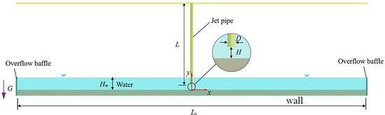
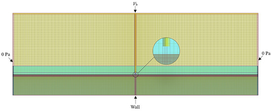
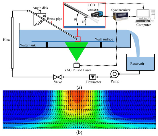
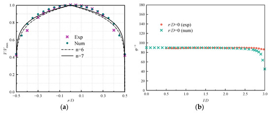
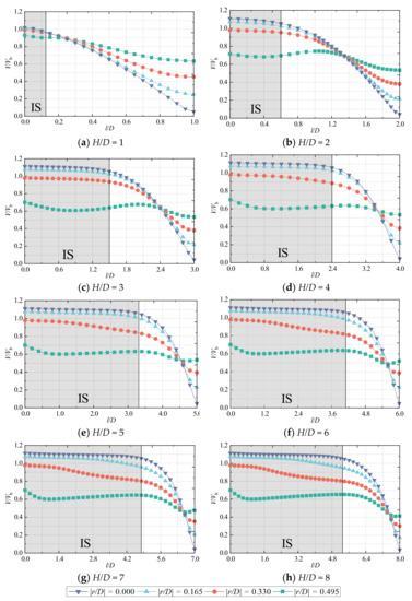
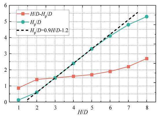
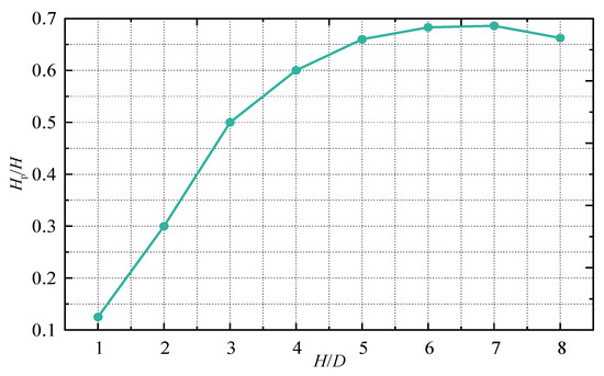
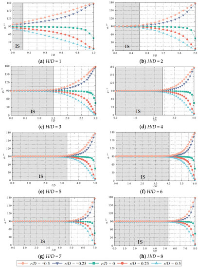
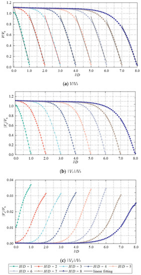
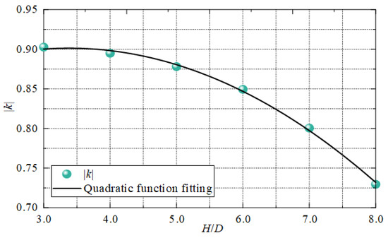
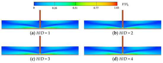
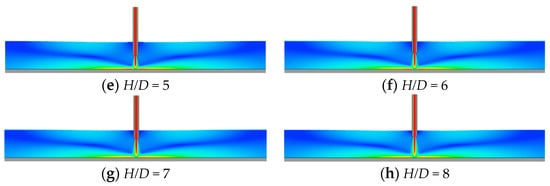
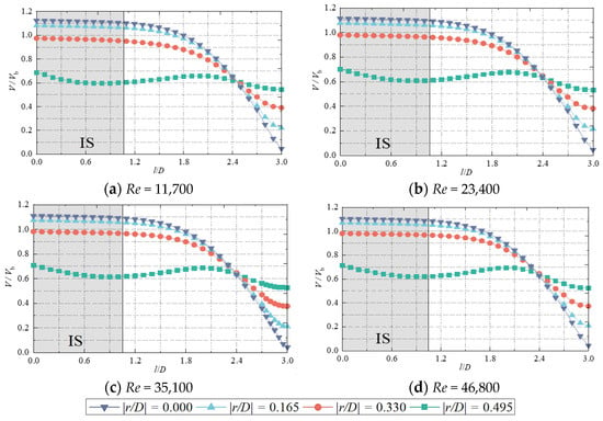
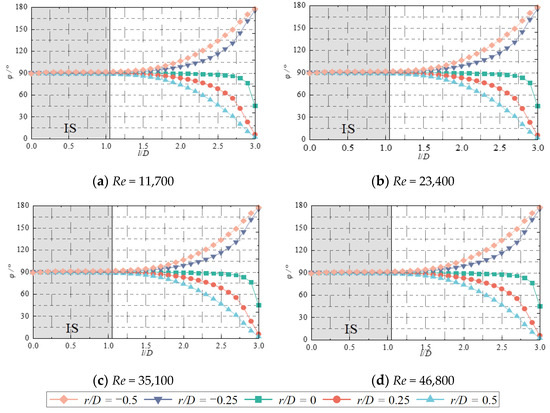
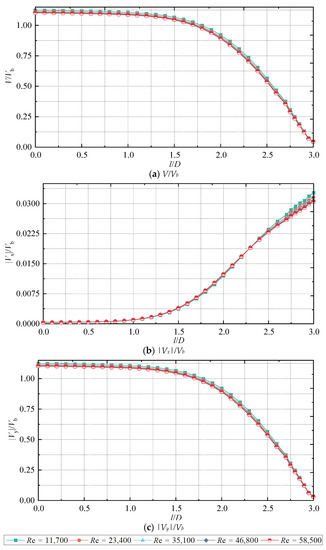
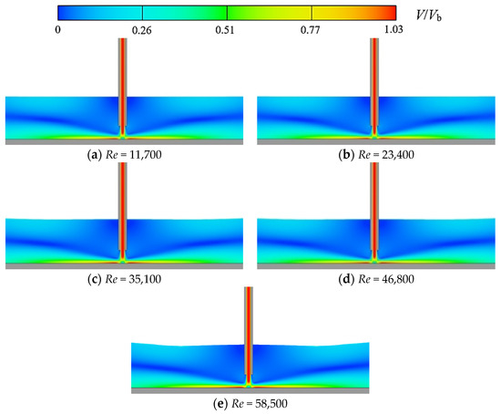


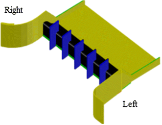
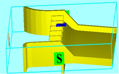
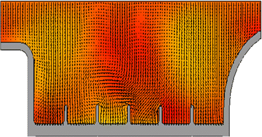
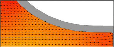
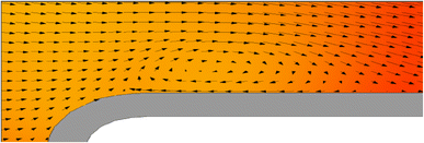
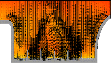
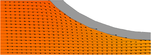
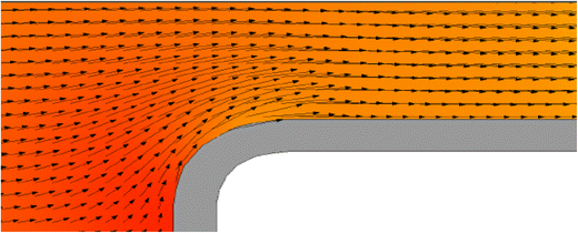
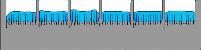
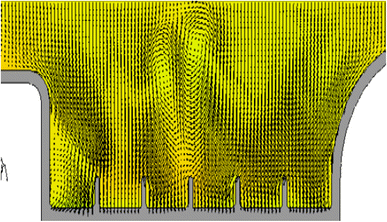
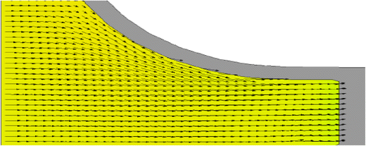
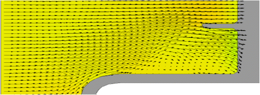

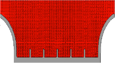
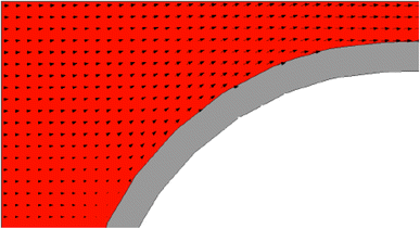
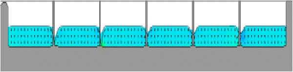


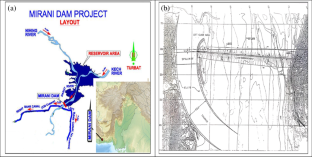
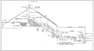
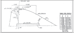
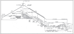
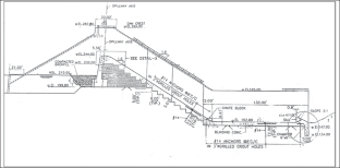
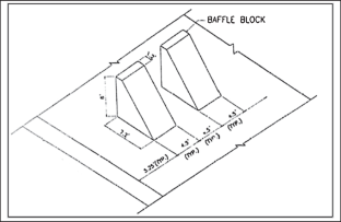
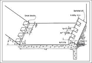
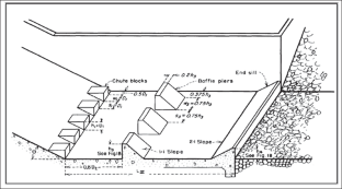
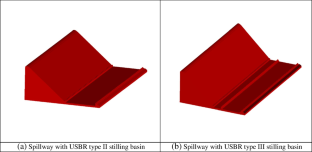

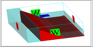
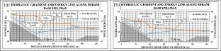
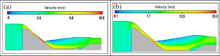
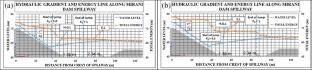
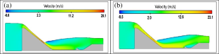

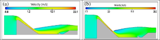
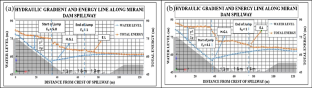
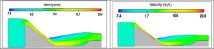
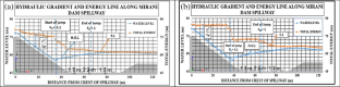
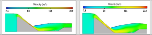


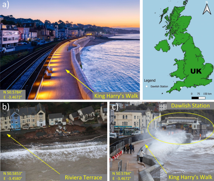
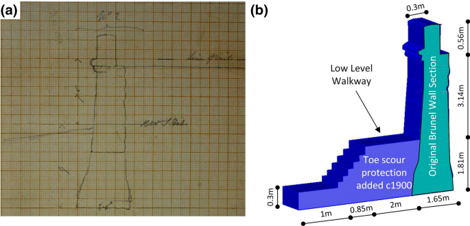
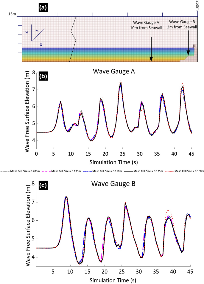
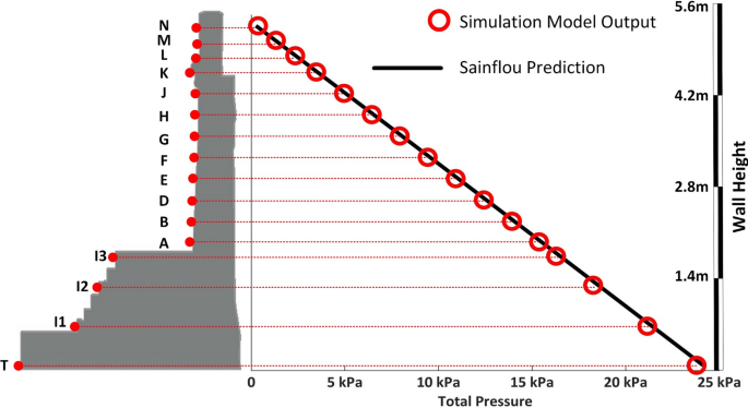
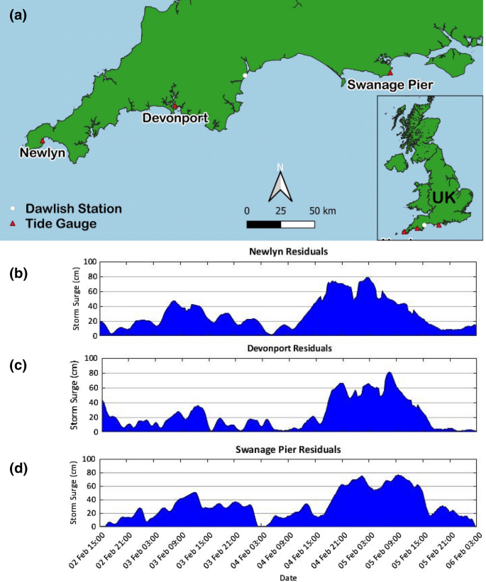
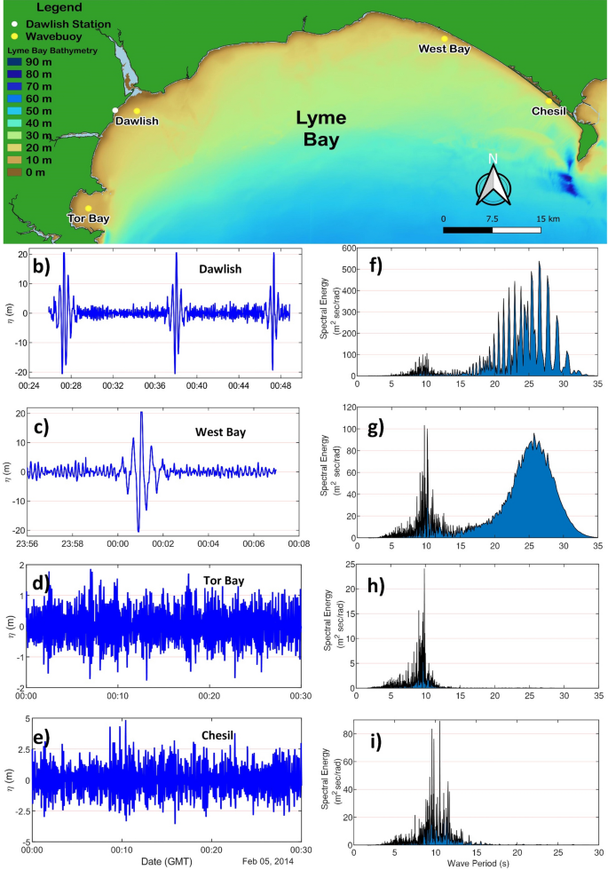
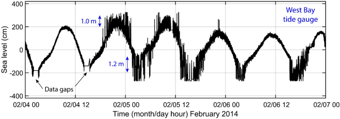
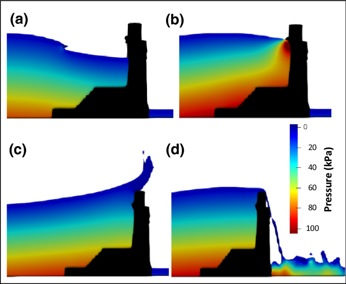
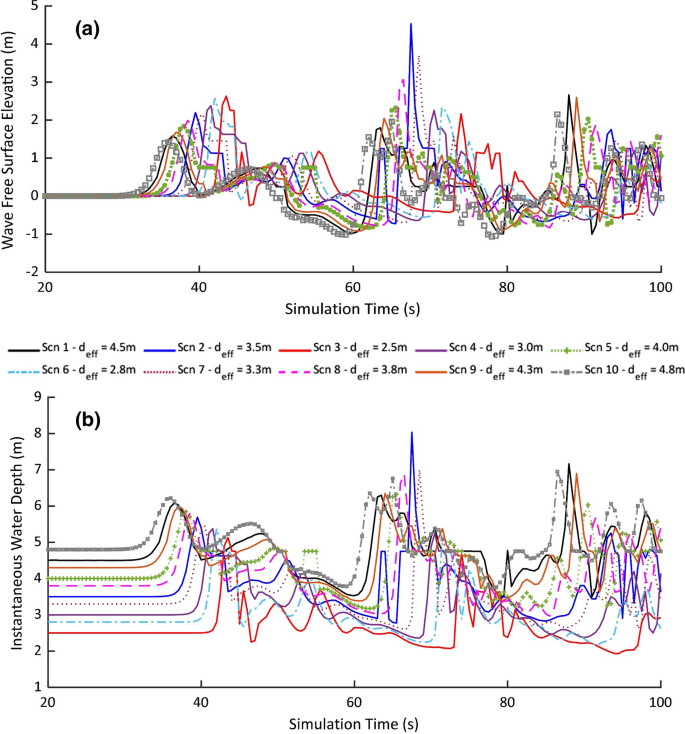
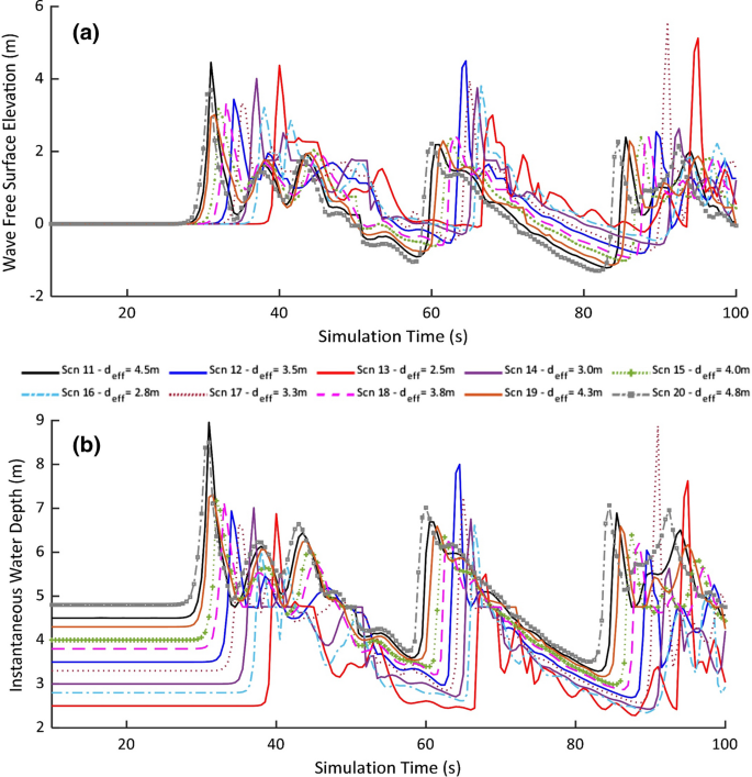
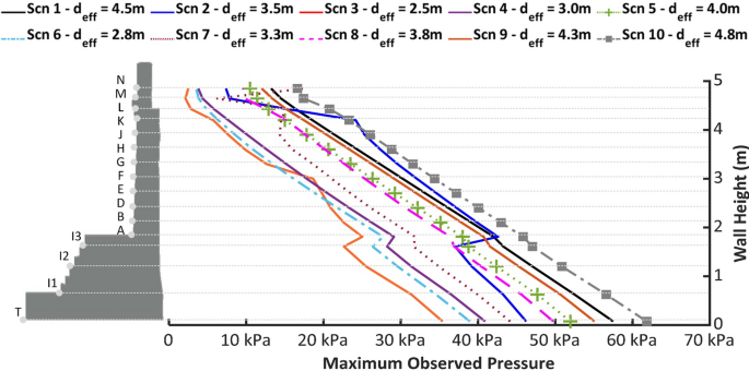
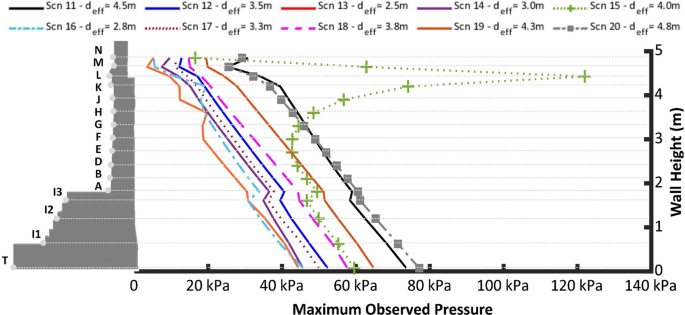
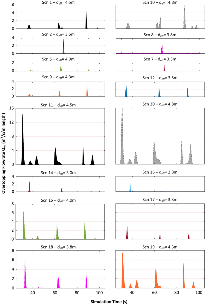
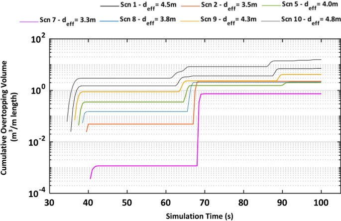
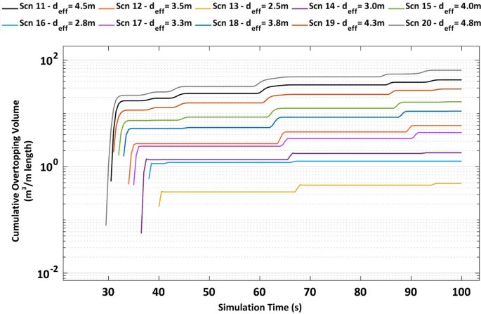


![Figure 2.1: Types of Landslides[2]](https://flow3d.co.kr/wp-content/uploads/Figure-2.1-Types-of-Landslides2.png)
![Figure 2.2: Landslide Glossary [2]](https://flow3d.co.kr/wp-content/uploads/Figure-2.2-Landslide-Glossary-2.png)