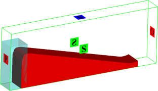
Figure 3 Simulation PTC pipes enhanced with copper foam and nanoparticles in FLOW-3D software.

다공성 미디어 및 나노유체에 의해 강화된 수집기로 태양광 CCHP 시스템의 최적화

Optimization of Solar CCHP Systems with Collector Enhanced by Porous Media and Nanofluid


Navid Tonekaboni,1Mahdi Feizbahr,2 Nima Tonekaboni,1Guang-Jun Jiang,3,4 and Hong-Xia Chen3,4

Abstract

태양열 집열기의 낮은 효율은 CCHP(Solar Combined Cooling, Heating, and Power) 사이클의 문제점 중 하나로 언급될 수 있습니다. 태양계를 개선하기 위해 나노유체와 다공성 매체가 태양열 집열기에 사용됩니다.

다공성 매질과 나노입자를 사용하는 장점 중 하나는 동일한 조건에서 더 많은 에너지를 흡수할 수 있다는 것입니다. 이 연구에서는 평균 일사량이 1b인 따뜻하고 건조한 지역의 600 m2 건물의 전기, 냉방 및 난방을 생성하기 위해 다공성 매질과 나노유체를 사용하여 태양열 냉난방 복합 발전(SCCHP) 시스템을 최적화했습니다.

본 논문에서는 침전물이 형성되지 않는 lb = 820 w/m2(이란) 정도까지 다공성 물질에서 나노유체의 최적량을 계산하였다. 이 연구에서 태양열 집열기는 구리 다공성 매체(95% 다공성)와 CuO 및 Al2O3 나노 유체로 향상되었습니다.

나노유체의 0.1%-0.6%가 작동 유체로 물에 추가되었습니다. 나노유체의 0.5%가 태양열 집열기 및 SCCHP 시스템에서 가장 높은 에너지 및 엑서지 효율 향상으로 이어지는 것으로 밝혀졌습니다.

본 연구에서 포물선형 집열기(PTC)의 최대 에너지 및 엑서지 효율은 각각 74.19% 및 32.6%입니다. 그림 1은 태양 CCHP의 주기를 정확하게 설명하기 위한 그래픽 초록으로 언급될 수 있습니다.

The low efficiency of solar collectors can be mentioned as one of the problems in solar combined cooling, heating, and power (CCHP) cycles. For improving solar systems, nanofluid and porous media are used in solar collectors. One of the advantages of using porous media and nanoparticles is to absorb more energy under the same conditions. In this research, a solar combined cooling, heating, and power (SCCHP) system has been optimized by porous media and nanofluid for generating electricity, cooling, and heating of a 600 m2 building in a warm and dry region with average solar radiation of Ib = 820 w/m2 in Iran. In this paper, the optimal amount of nanofluid in porous materials has been calculated to the extent that no sediment is formed. In this study, solar collectors were enhanced with copper porous media (95% porosity) and CuO and Al2O3 nanofluids. 0.1%–0.6% of the nanofluids were added to water as working fluids; it is found that 0.5% of the nanofluids lead to the highest energy and exergy efficiency enhancement in solar collectors and SCCHP systems. Maximum energy and exergy efficiency of parabolic thermal collector (PTC) riches in this study are 74.19% and 32.6%, respectively. Figure 1 can be mentioned as a graphical abstract for accurately describing the cycle of solar CCHP.

1. Introduction

Due to the increase in energy consumption, the use of clean energy is one of the important goals of human societies. In the last four decades, the use of cogeneration cycles has increased significantly due to high efficiency. Among clean energy, the use of solar energy has become more popular due to its greater availability [1]. Low efficiency of energy production, transmission, and distribution system makes a new system to generate simultaneously electricity, heating, and cooling as an essential solution to be widely used. The low efficiency of the electricity generation, transmission, and distribution system makes the CCHP system a basic solution to eliminate waste of energy. CCHP system consists of a prime mover (PM), a power generator, a heat recovery system (produce extra heating/cooling/power), and thermal energy storage (TES) [2]. Solar combined cooling, heating, and power (SCCHP) has been started three decades ago. SCCHP is a system that receives its propulsive force from solar energy; in this cycle, solar collectors play the role of propulsive for generating power in this system [3].

Increasing the rate of energy consumption in the whole world because of the low efficiency of energy production, transmission, and distribution system causes a new cogeneration system to generate electricity, heating, and cooling energy as an essential solution to be widely used. Building energy utilization fundamentally includes power required for lighting, home electrical appliances, warming and cooling of building inside, and boiling water. Domestic usage contributes to an average of 35% of the world’s total energy consumption [4].

Due to the availability of solar energy in all areas, solar collectors can be used to obtain the propulsive power required for the CCHP cycle. Solar energy is the main source of energy in renewable applications. For selecting a suitable area to use solar collectors, annual sunshine hours, the number of sunny days, minus temperature and frosty days, and the windy status of the region are essentially considered [5]. Iran, with an average of more than 300 sunny days, is one of the suitable countries to use solar energy. Due to the fact that most of the solar radiation is in the southern regions of Iran, also the concentration of cities is low in these areas, and transmission lines are far apart, one of the best options is to use CCHP cycles based on solar collectors [6]. One of the major problems of solar collectors is their low efficiency [7]. Low efficiency increases the area of collectors, which increases the initial cost of solar systems and of course increases the initial payback period. To increase the efficiency of solar collectors and improve their performance, porous materials and nanofluids are used to increase their workability.

There are two ways to increase the efficiency of solar collectors and mechanical and fluid improvement. In the first method, using porous materials or helical filaments inside the collector pipes causes turbulence of the flow and increases heat transfer. In the second method, using nanofluids or salt and other materials increases the heat transfer of water. The use of porous materials has grown up immensely over the past twenty years. Porous materials, especially copper porous foam, are widely used in solar collectors. Due to the high contact surface area, porous media are appropriate candidates for solar collectors [8]. A number of researchers investigated Solar System performance in accordance with energy and exergy analyses. Zhai et al. [9] reviewed the performance of a small solar-powered system in which the energy efficiency was 44.7% and the electrical efficiency was 16.9%.

Abbasi et al. [10] proposed an innovative multiobjective optimization to optimize the design of a cogeneration system. Results showed the CCHP system based on an internal diesel combustion engine was the applicable alternative at all regions with different climates. The diesel engine can supply the electrical requirement of 31.0% and heating demand of 3.8% for building.

Jiang et al. [11] combined the experiment and simulation together to analyze the performance of a cogeneration system. Moreover, some research focused on CCHP systems using solar energy. It integrated sustainable and renewable technologies in the CCHP, like PV, Stirling engine, and parabolic trough collector (PTC) [21215].

Wang et al. [16] optimized a cogeneration solar cooling system with a Rankine cycle and ejector to reach the maximum total system efficiency of 55.9%. Jing et al. analyzed a big-scale building with the SCCHP system and auxiliary heaters to produced electrical, cooling, and heating power. The maximum energy efficiency reported in their work is 46.6% [17]. Various optimization methods have been used to improve the cogeneration system, minimum system size, and performance, such as genetic algorithm [1819].

Hirasawa et al. [20] investigated the effect of using porous media to reduce thermal waste in solar systems. They used the high-porosity metal foam on top of the flat plate solar collector and observed that thermal waste decreased by 7% due to natural heat transfer. Many researchers study the efficiency improvement of the solar collector by changing the collector’s shapes or working fluids. However, the most effective method is the use of nanofluids in the solar collector as working fluid [21]. In the experimental study done by Jouybari et al. [22], the efficiency enhancement up to 8.1% was achieved by adding nanofluid in a flat plate collector. In this research, by adding porous materials to the solar collector, collector efficiency increased up to 92% in a low flow regime. Subramani et al. [23] analyzed the thermal performance of the parabolic solar collector with Al2O3 nanofluid. They conducted their experiments with Reynolds number range 2401 to 7202 and mass flow rate 0.0083 to 0.05 kg/s. The maximum efficiency improvement in this experiment was 56% at 0.05 kg/s mass flow rate.

Shojaeizadeh et al. [24] investigated the analysis of the second law of thermodynamic on the flat plate solar collector using Al2O3/water nanofluid. Their research showed that energy efficiency rose up to 1.9% and the exergy efficiency increased by a maximum of 0.72% compared to pure water. Tiwari et al. [25] researched on the thermal performance of solar flat plate collectors for working fluid water with different nanofluids. The result showed that using 1.5% (optimum) particle volume fraction of Al2O3 nanofluid as an absorbing medium causes the thermal efficiency to enhance up to 31.64%.

The effect of porous media and nanofluids on solar collectors has already been investigated in the literature but the SCCHP system with a collector embedded by both porous media and nanofluid for enhancing the ratio of nanoparticle in nanofluid for preventing sedimentation was not discussed. In this research, the amount of energy and exergy of the solar CCHP cycles with parabolic solar collectors in both base and improved modes with a porous material (copper foam with 95% porosity) and nanofluid with different ratios of nanoparticles was calculated. In the first step, it is planned to design a CCHP system based on the required load, and, in the next step, it will analyze the energy and exergy of the system in a basic and optimize mode. In the optimize mode, enhanced solar collectors with porous material and nanofluid in different ratios (0.1%–0.7%) were used to optimize the ratio of nanofluids to prevent sedimentation.

2. Cycle Description

CCHP is one of the methods to enhance energy efficiency and reduce energy loss and costs. The SCCHP system used a solar collector as a prime mover of the cogeneration system and assisted the boiler to generate vapor for the turbine. Hot water flows from the expander to the absorption chiller in summer or to the radiator or fan coil in winter. Finally, before the hot water wants to flow back to the storage tank, it flows inside a heat exchanger for generating domestic hot water [26].

For designing of solar cogeneration system and its analysis, it is necessary to calculate the electrical, heating (heating load is the load required for the production of warm water and space heating), and cooling load required for the case study considered in a residential building with an area of 600 m2 in the warm region of Iran (Zahedan). In Table 1, the average of the required loads is shown for the different months of a year (average of electrical, heating, and cooling load calculated with CARRIER software).Table 1 The average amount of electric charges, heating load, and cooling load used in the different months of the year in the city of Zahedan for a residential building with 600 m2.

According to Table 1, the maximum magnitude of heating, cooling, and electrical loads is used to calculate the cogeneration system. The maximum electric load is 96 kW, the maximum amount of heating load is 62 kW, and the maximum cooling load is 118 kW. Since the calculated loads are average, all loads increased up to 10% for the confidence coefficient. With the obtained values, the solar collector area and other cogeneration system components are calculated. The cogeneration cycle is capable of producing 105 kW electric power, 140 kW cooling capacity, and 100 kW heating power.

2.1. System Analysis Equations

An analysis is done by considering the following assumptions:(1)The system operates under steady-state conditions(2)The system is designed for the warm region of Iran (Zahedan) with average solar radiation Ib = 820 w/m2(3)The pressure drops in heat exchangers, separators, storage tanks, and pipes are ignored(4)The pressure drop is negligible in all processes and no expectable chemical reactions occurred in the processes(5)Potential, kinetic, and chemical exergy are not considered due to their insignificance(6)Pumps have been discontinued due to insignificance throughout the process(7)All components are assumed adiabatic

Schematic shape of the cogeneration cycle is shown in Figure 1 and all data are given in Table 2.

Figure 1 Schematic shape of the cogeneration cycle.Table 2 Temperature and humidity of different points of system.

Based on the first law of thermodynamic, energy analysis is based on the following steps.

First of all, the estimated solar radiation energy on collector has been calculated:where α is the heat transfer enhancement coefficient based on porous materials added to the collector’s pipes. The coefficient α is increased by the porosity percentage, the type of porous material (in this case, copper with a porosity percentage of 95), and the flow of fluid to the collector equation.

Collector efficiency is going to be calculated by the following equation [9]:

Total energy received by the collector is given by [9]

Also, the auxiliary boiler heat load is [2]

Energy consumed from vapor to expander is calculated by [2]

The power output form by the screw expander [9]:

The efficiency of the expander is 80% in this case [11].

In this step, cooling and heating loads were calculated and then, the required heating load to reach sanitary hot water will be calculated as follows:

First step: calculating the cooling load with the following equation [9]:

Second step: calculating heating loads [9]:

Then, calculating the required loud for sanitary hot water will be [9]

According to the above-mentioned equations, efficiency is [9]

In the third step, calculated exergy analysis as follows.

First, the received exergy collector from the sun is calculated [9]:

In the previous equation, f is the constant of air dilution.

The received exergy from the collector is [9]

In the case of using natural gas in an auxiliary heater, the gas exergy is calculated from the following equation [12]:

Delivering exergy from vapor to expander is calculated with the following equation [9]:

In the fourth step, the exergy in cooling and heating is calculated by the following equation:

Cooling exergy in summer is calculated [9]:

Heating exergy in winter is calculated [9]:

In the last step based on thermodynamic second law, exergy efficiency has been calculated from the following equation and the above-mentioned calculated loads [9]:

3. Porous Media

The porous medium that filled the test section is copper foam with a porosity of 95%. The foams are determined in Figure 2 and also detailed thermophysical parameters and dimensions are shown in Table 3.

Figure 2 Copper foam with a porosity of 95%.Table 3 Thermophysical parameters and dimensions of copper foam.

In solar collectors, copper porous materials are suitable for use at low temperatures and have an easier and faster manufacturing process than ceramic porous materials. Due to the high coefficient conductivity of copper, the use of copper metallic foam to increase heat transfer is certainly more efficient in solar collectors.

Porous media and nanofluid in solar collector’s pipes were simulated in FLOW-3D software using the finite-difference method [27]. Nanoparticles Al2O3 and CUO are mostly used in solar collector enhancement. In this research, different concentrations of nanofluid are added to the parabolic solar collectors with porous materials (copper foam with porosity of 95%) to achieve maximum heat transfer in the porous materials before sedimentation. After analyzing PTC pipes with the nanofluid flow in FLOW-3D software, for energy and exergy efficiency analysis, Carrier software results were used as EES software input. Simulation PTC with porous media inside collector pipe and nanofluids sedimentation is shown in Figure 3.

Figure 3 Simulation PTC pipes enhanced with copper foam and nanoparticles in FLOW-3D software.

3.1. Nano Fluid

In this research, copper and silver nanofluids (Al2O3, CuO) have been added with percentages of 0.1%–0.7% as the working fluids. The nanoparticle properties are given in Table 4. Also, system constant parameters are presented in Table 4, which are available as default input in the EES software.Table 4 Properties of the nanoparticles [9].

System constant parameters for input in the software are shown in Table 5.Table 5 System constant parameters.

The thermal properties of the nanofluid can be obtained from equations (18)–(21). The basic fluid properties are indicated by the index (bf) and the properties of the nanoparticle silver with the index (np).

The density of the mixture is shown in the following equation [28]:where ρ is density and ϕ is the nanoparticles volume fraction.

The specific heat capacity is calculated from the following equation [29]:

The thermal conductivity of the nanofluid is calculated from the following equation [29]:

The parameter β is the ratio of the nanolayer thickness to the original particle radius and, usually, this parameter is taken equal to 0.1 for the calculated thermal conductivity of the nanofluids.

The mixture viscosity is calculated as follows [30]:

In all equations, instead of water properties, working fluids with nanofluid are used. All of the above equations and parameters are entered in the EES software for calculating the energy and exergy of solar collectors and the SCCHP cycle. All calculation repeats for both nanofluids with different concentrations of nanofluid in the solar collector’s pipe.

4. Results and Discussion

In the present study, relations were written according to Wang et al. [16] and the system analysis was performed to ensure the correctness of the code. The energy and exergy charts are plotted based on the main values of the paper and are shown in Figures 4 and 5. The error rate in this simulation is 1.07%.

Figure 4 Verification charts of energy analysis results.

Figure 5 Verification charts of exergy analysis results.

We may also investigate the application of machine learning paradigms [3141] and various hybrid, advanced optimization approaches that are enhanced in terms of exploration and intensification [4255], and intelligent model studies [5661] as well, for example, methods such as particle swarm optimizer (PSO) [6062], differential search (DS) [63], ant colony optimizer (ACO) [616465], Harris hawks optimizer (HHO) [66], grey wolf optimizer (GWO) [5367], differential evolution (DE) [6869], and other fusion and boosted systems [4146485054557071].

At the first step, the collector is modified with porous copper foam material. 14 cases have been considered for the analysis of the SCCHP system (Table 6). It should be noted that the adding of porous media causes an additional pressure drop inside the collector [922263072]. All fourteen cases use copper foam with a porosity of 95 percent. To simulate the effect of porous materials and nanofluids, the first solar PTC pipes have been simulated in the FLOW-3D software and then porous media (copper foam with porosity of 95%) and fluid flow with nanoparticles (AL2O3 and CUO) are generated in the software. After analyzing PTC pipes in FLOW-3D software, for analyzing energy and exergy efficiency, software outputs were used as EES software input for optimization ratio of sedimentation and calculating energy and exergy analyses.Table 6 Collectors with different percentages of nanofluids and porous media.

In this research, an enhanced solar collector with both porous media and Nanofluid is investigated. In the present study, 0.1–0.5% CuO and Al2O3 concentration were added to the collector fully filled by porous media to achieve maximum energy and exergy efficiencies of solar CCHP systems. All steps of the investigation are shown in Table 6.

Energy and exergy analyses of parabolic solar collectors and SCCHP systems are shown in Figures 6 and 7.

Figure 6 Energy and exergy efficiencies of the PTC with porous media and nanofluid.

Figure 7 Energy and exergy efficiency of the SCCHP.

Results show that the highest energy and exergy efficiencies are 74.19% and 32.6%, respectively, that is achieved in Step 12 (parabolic collectors with filled porous media and 0.5% Al2O3). In the second step, the maximum energy efficiency of SCCHP systems with fourteen steps of simulation are shown in Figure 7.

In the second step, where 0.1, −0.6% of the nanofluids were added, it is found that 0.5% leads to the highest energy and exergy efficiency enhancement in solar collectors and SCCHP systems. Using concentrations more than 0.5% leads to sediment in the solar collector’s pipe and a decrease of porosity in the pipe [73]. According to Figure 7, maximum energy and exergy efficiencies of SCCHP are achieved in Step 12. In this step energy efficiency is 54.49% and exergy efficiency is 18.29%. In steps 13 and 14, with increasing concentration of CUO and Al2O3 nanofluid solution in porous materials, decreasing of energy and exergy efficiency of PTC and SCCHP system at the same time happened. This decrease in efficiency is due to the formation of sediment in the porous material. Calculations and simulations have shown that porous materials more than 0.5% nanofluids inside the collector pipe cause sediment and disturb the porosity of porous materials and pressure drop and reduce the coefficient of performance of the cogeneration system. Most experience showed that CUO and AL2O3 nanofluids with less than 0.6% percent solution are used in the investigation on the solar collectors at low temperatures and discharges [74]. One of the important points of this research is that the best ratio of nanofluids in the solar collector with a low temperature is 0.5% (AL2O3 and CUO); with this replacement, the cost of solar collectors and SCCHP cycle is reduced.

5. Conclusion and Future Directions

In the present study, ways for increasing the efficiency of solar collectors in order to enhance the efficiency of the SCCHP cycle are examined. The research is aimed at adding both porous materials and nanofluids for estimating the best ratio of nanofluid for enhanced solar collector and protecting sedimentation in porous media. By adding porous materials (copper foam with porosity of 95%) and 0.5% nanofluids together, high efficiency in solar parabolic collectors can be achieved. The novelty in this research is the addition of both nanofluids and porous materials and calculating the best ratio for preventing sedimentation and pressure drop in solar collector’s pipe. In this study, it was observed that, by adding 0.5% of AL2O3 nanofluid in working fluids, the energy efficiency of PTC rises to 74.19% and exergy efficiency is grown up to 32.6%. In SCCHP cycle, energy efficiency is 54.49% and exergy efficiency is 18.29%.

In this research, parabolic solar collectors fully filled by porous media (copper foam with a porosity of 95) are investigated. In the next step, parabolic solar collectors in the SCCHP cycle were simultaneously filled by porous media and different percentages of Al2O3 and CuO nanofluid. At this step, values of 0.1% to 0.6% of each nanofluid were added to the working fluid, and the efficiency of the energy and exergy of the collectors and the SCCHP cycle were determined. In this case, nanofluid and the porous media were used together in the solar collector and maximum efficiency achieved. 0.5% of both nanofluids were used to achieve the biggest efficiency enhancement.

In the present study, as expected, the highest efficiency is for the parabolic solar collector fully filled by porous material (copper foam with a porosity of 95%) and 0.5% Al2O3. Results of the present study are as follows:(1)The average enhancement of collectors’ efficiency using porous media and nanofluids is 28%.(2)Solutions with 0.1 to 0.5% of nanofluids (CuO and Al2O3) are used to prevent collectors from sediment occurrence in porous media.(3)Collector of solar cogeneration cycles that is enhanced by both porous media and nanofluid has higher efficiency, and the stability of output temperature is more as well.(4)By using 0.6% of the nanofluids in the enhanced parabolic solar collectors with copper porous materials, sedimentation occurs and makes a high-pressure drop in the solar collector’s pipe which causes decrease in energy efficiency.(5)Average enhancement of SCCHP cycle efficiency is enhanced by both porous media and nanofluid 13%.

Nomenclature

:Solar radiation
a:Heat transfer augmentation coefficient
A:Solar collector area
Bf:Basic fluid
:Specific heat capacity of the nanofluid
F:Constant of air dilution
:Thermal conductivity of the nanofluid
:Thermal conductivity of the basic fluid
:Viscosity of the nanofluid
:Viscosity of the basic fluid
:Collector efficiency
:Collector energy receives
:Auxiliary boiler heat
:Expander energy
:Gas energy
:Screw expander work
:Cooling load, in kilowatts
:Heating load, in kilowatts
:Solar radiation energy on collector, in Joule
:Sanitary hot water load
Np:Nanoparticle
:Energy efficiency
:Heat exchanger efficiency
:Sun exergy
:Collector exergy
:Natural gas exergy
:Expander exergy
:Cooling exergy
:Heating exergy
:Exergy efficiency
:Steam mass flow rate
:Hot water mass flow rate
:Specific heat capacity of water
:Power output form by the screw expander
Tam:Average ambient temperature
:Density of the mixture.

Greek symbols

ρ:Density
ϕ:Nanoparticles volume fraction
β:Ratio of the nanolayer thickness.

Abbreviations

CCHP:Combined cooling, heating, and power
EES:Engineering equation solver.

Data Availability

For this study, data were generated by CARRIER software for the average electrical, heating, and cooling load of a residential building with 600 m2 in the city of Zahedan, Iran.

Conflicts of Interest

The authors declare that they have no conflicts of interest.

Acknowledgments

This work was partially supported by the National Natural Science Foundation of China under Contract no. 71761030 and Natural Science Foundation of Inner Mongolia under Contract no. 2019LH07003.

References

  1. A. Fudholi and K. Sopian, “Review on solar collector for agricultural produce,” International Journal of Power Electronics and Drive Systems (IJPEDS), vol. 9, no. 1, p. 414, 2018.View at: Publisher Site | Google Scholar
  2. G. Yang and X. Zhai, “Optimization and performance analysis of solar hybrid CCHP systems under different operation strategies,” Applied Thermal Engineering, vol. 133, pp. 327–340, 2018.View at: Publisher Site | Google Scholar
  3. J. Wang, Z. Han, and Z. Guan, “Hybrid solar-assisted combined cooling, heating, and power systems: a review,” Renewable and Sustainable Energy Reviews, vol. 133, p. 110256, 2020.View at: Publisher Site | Google Scholar
  4. Y. Tian and C. Y. Zhao, “A review of solar collectors and thermal energy storage in solar thermal applications,” Applied Energy, vol. 104, pp. 538–553, 2013.View at: Publisher Site | Google Scholar
  5. J. M. Hassan, Q. J. Abdul-Ghafour, and M. F. Mohammed, “CFD simulation of enhancement techniques in flat plate solar water collectors,” Al-Nahrain Journal for Engineering Sciences, vol. 20, no. 3, pp. 751–761, 2017.View at: Google Scholar
  6. M. Jahangiri, O. Nematollahi, A. Haghani, H. A. Raiesi, and A. Alidadi Shamsabadi, “An optimization of energy cost of clean hybrid solar-wind power plants in Iran,” International Journal of Green Energy, vol. 16, no. 15, pp. 1422–1435, 2019.View at: Publisher Site | Google Scholar
  7. I. H. Yılmaz and A. Mwesigye, “Modeling, simulation and performance analysis of parabolic trough solar collectors: a comprehensive review,” Applied Energy, vol. 225, pp. 135–174, 2018.View at: Google Scholar
  8. F. Wang, J. Tan, and Z. Wang, “Heat transfer analysis of porous media receiver with different transport and thermophysical models using mixture as feeding gas,” Energy Conversion and Management, vol. 83, pp. 159–166, 2014.View at: Publisher Site | Google Scholar
  9. H. Zhai, Y. J. Dai, J. Y. Wu, and R. Z. Wang, “Energy and exergy analyses on a novel hybrid solar heating, cooling and power generation system for remote areas,” Applied Energy, vol. 86, no. 9, pp. 1395–1404, 2009.View at: Publisher Site | Google Scholar
  10. M. H. Abbasi, H. Sayyaadi, and M. Tahmasbzadebaie, “A methodology to obtain the foremost type and optimal size of the prime mover of a CCHP system for a large-scale residential application,” Applied Thermal Engineering, vol. 135, pp. 389–405, 2018.View at: Google Scholar
  11. R. Jiang, F. G. F. Qin, X. Yang, S. Huang, and B. Chen, “Performance analysis of a liquid absorption dehumidifier driven by jacket-cooling water of a diesel engine in a CCHP system,” Energy and Buildings, vol. 163, pp. 70–78, 2018.View at: Publisher Site | Google Scholar
  12. F. A. Boyaghchi and M. Chavoshi, “Monthly assessments of exergetic, economic and environmental criteria and optimization of a solar micro-CCHP based on DORC,” Solar Energy, vol. 166, pp. 351–370, 2018.View at: Publisher Site | Google Scholar
  13. F. A. Boyaghchi and M. Chavoshi, “Multi-criteria optimization of a micro solar-geothermal CCHP system applying water/CuO nanofluid based on exergy, exergoeconomic and exergoenvironmental concepts,” Applied Thermal Engineering, vol. 112, pp. 660–675, 2017.View at: Publisher Site | Google Scholar
  14. B. Su, W. Han, Y. Chen, Z. Wang, W. Qu, and H. Jin, “Performance optimization of a solar assisted CCHP based on biogas reforming,” Energy Conversion and Management, vol. 171, pp. 604–617, 2018.View at: Publisher Site | Google Scholar
  15. F. A. Al-Sulaiman, F. Hamdullahpur, and I. Dincer, “Performance assessment of a novel system using parabolic trough solar collectors for combined cooling, heating, and power production,” Renewable Energy, vol. 48, pp. 161–172, 2012.View at: Publisher Site | Google Scholar
  16. J. Wang, Y. Dai, L. Gao, and S. Ma, “A new combined cooling, heating and power system driven by solar energy,” Renewable Energy, vol. 34, no. 12, pp. 2780–2788, 2009.View at: Publisher Site | Google Scholar
  17. Y.-Y. Jing, H. Bai, J.-J. Wang, and L. Liu, “Life cycle assessment of a solar combined cooling heating and power system in different operation strategies,” Applied Energy, vol. 92, pp. 843–853, 2012.View at: Publisher Site | Google Scholar
  18. J.-J. Wang, Y.-Y. Jing, and C.-F. Zhang, “Optimization of capacity and operation for CCHP system by genetic algorithm,” Applied Energy, vol. 87, no. 4, pp. 1325–1335, 2010.View at: Publisher Site | Google Scholar
  19. L. Ali, “LDA–GA–SVM: improved hepatocellular carcinoma prediction through dimensionality reduction and genetically optimized support vector machine,” Neural Computing and Applications, vol. 87, pp. 1–10, 2020.View at: Google Scholar
  20. S. Hirasawa, R. Tsubota, T. Kawanami, and K. Shirai, “Reduction of heat loss from solar thermal collector by diminishing natural convection with high-porosity porous medium,” Solar Energy, vol. 97, pp. 305–313, 2013.View at: Publisher Site | Google Scholar
  21. E. Bellos, C. Tzivanidis, and Z. Said, “A systematic parametric thermal analysis of nanofluid-based parabolic trough solar collectors,” Sustainable Energy Technologies and Assessments, vol. 39, p. 100714, 2020.View at: Publisher Site | Google Scholar
  22. H. J. Jouybari, S. Saedodin, A. Zamzamian, M. E. Nimvari, and S. Wongwises, “Effects of porous material and nanoparticles on the thermal performance of a flat plate solar collector: an experimental study,” Renewable Energy, vol. 114, pp. 1407–1418, 2017.View at: Publisher Site | Google Scholar
  23. J. Subramani, P. K. Nagarajan, S. Wongwises, S. A. El-Agouz, and R. Sathyamurthy, “Experimental study on the thermal performance and heat transfer characteristics of solar parabolic trough collector using Al2O3 nanofluids,” Environmental Progress & Sustainable Energy, vol. 37, no. 3, pp. 1149–1159, 2018.View at: Publisher Site | Google Scholar
  24. E. Shojaeizadeh, F. Veysi, and A. Kamandi, “Exergy efficiency investigation and optimization of an Al2O3-water nanofluid based Flat-plate solar collector,” Energy and Buildings, vol. 101, pp. 12–23, 2015.View at: Publisher Site | Google Scholar
  25. A. K. Tiwari, P. Ghosh, and J. Sarkar, “Solar water heating using nanofluids–a comprehensive overview and environmental impact analysis,” International Journal of Emerging Technology and Advanced Engineering, vol. 3, no. 3, pp. 221–224, 2013.View at: Google Scholar
  26. D. R. Rajendran, E. Ganapathy Sundaram, P. Jawahar, V. Sivakumar, O. Mahian, and E. Bellos, “Review on influencing parameters in the performance of concentrated solar power collector based on materials, heat transfer fluids and design,” Journal of Thermal Analysis and Calorimetry, vol. 140, no. 1, pp. 33–51, 2020.View at: Publisher Site | Google Scholar
  27. M. Feizbahr, C. Kok Keong, F. Rostami, and M. Shahrokhi, “Wave energy dissipation using perforated and non perforated piles,” International Journal of Engineering, vol. 31, no. 2, pp. 212–219, 2018.View at: Google Scholar
  28. K. Khanafer and K. Vafai, “A critical synthesis of thermophysical characteristics of nanofluids,” International Journal of Heat and Mass Transfer, vol. 54, no. 19-20, pp. 4410–4428, 2011.View at: Publisher Site | Google Scholar
  29. K. Farhana, K. Kadirgama, M. M. Rahman et al., “Improvement in the performance of solar collectors with nanofluids – a state-of-the-art review,” Nano-Structures & Nano-Objects, vol. 18, p. 100276, 2019.View at: Publisher Site | Google Scholar
  30. M. Turkyilmazoglu, “Condensation of laminar film over curved vertical walls using single and two-phase nanofluid models,” European Journal of Mechanics-B/Fluids, vol. 65, pp. 184–191, 2017.View at: Publisher Site | Google Scholar
  31. X. Zhang, J. Wang, T. Wang, R. Jiang, J. Xu, and L. Zhao, “Robust feature learning for adversarial defense via hierarchical feature alignment,” Information Sciences, vol. 2020, 2020.View at: Google Scholar
  32. X. Zhang, T. Wang, W. Luo, and P. Huang, “Multi-level fusion and attention-guided CNN for image dehazing,” IEEE Transactions on Circuits and Systems for Video Technology, vol. 1, 2020.View at: Publisher Site | Google Scholar
  33. X. Zhang, M. Fan, D. Wang, P. Zhou, and D. Tao, “Top-k feature selection framework using robust 0-1 integer programming,” IEEE Transactions on Neural Networks and Learning Systems, vol. 1, pp. 1–15, 2020.View at: Publisher Site | Google Scholar
  34. X. Zhang, D. Wang, Z. Zhou, and Y. Ma, “Robust low-rank tensor recovery with rectification and alignment,” IEEE Transactions on Pattern Analysis and Machine Intelligence, vol. 43, no. 1, pp. 238–255, 2019.View at: Google Scholar
  35. X. Zhang, R. Jiang, T. Wang, and J. Wang, “Recursive neural network for video deblurring,” IEEE Transactions on Circuits and Systems for Video Technology, vol. 1, 2020.View at: Publisher Site | Google Scholar
  36. X. Zhang, T. Wang, J. Wang, G. Tang, and L. Zhao, “Pyramid channel-based feature attention network for image dehazing,” Computer Vision and Image Understanding, vol. 1, 2020.View at: Google Scholar
  37. M. Mirmozaffari, “Machine learning algorithms based on an optimization model,” 2020.View at: Google Scholar
  38. M. Mirmozaffari, M. Yazdani, A. Boskabadi, H. Ahady Dolatsara, K. Kabirifar, and N. Amiri Golilarz, “A novel machine learning approach combined with optimization models for eco-efficiency evaluation,” Applied Sciences, vol. 10, no. 15, p. 5210, 2020.View at: Publisher Site | Google Scholar
  39. M. Vosoogha and A. Addeh, “An intelligent power prediction method for wind energy generation based on optimized fuzzy system,” Computational Research Progress in Applied Science & Engineering (CRPASE), vol. 5, pp. 34–43, 2019.View at: Google Scholar
  40. A. Javadi, N. Mikaeilvand, and H. Hosseinzdeh, “Presenting a new method to solve partial differential equations using a group search optimizer method (GSO),” Computational Research Progress in Applied Science and Engineering, vol. 4, no. 1, pp. 22–26, 2018.View at: Google Scholar
  41. F. J. Golrokh, Gohar Azeem, and A. Hasan, “Eco-efficiency evaluation in cement industries: DEA malmquist productivity index using optimization models,” ENG Transactions, vol. 1, pp. 1–8, 2020.View at: Google Scholar
  42. H. Yu, “Dynamic Gaussian bare-bones fruit fly optimizers with abandonment mechanism: method and analysis,” Engineering with Computers, vol. 1, pp. 1–29, 2020.View at: Google Scholar
  43. C. Yu, “SGOA: annealing-behaved grasshopper optimizer for global tasks,” Engineering with Computers, vol. 1, pp. 1–28, 2021.View at: Google Scholar
  44. W. Shan, Z. Qiao, A. A. Heidari, H. Chen, H. Turabieh, and Y. Teng, “Double adaptive weights for stabilization of moth flame optimizer: balance analysis, engineering cases, and medical diagnosis,” Knowledge-Based Systems, vol. 1, p. 106728, 2020.View at: Google Scholar
  45. J. Tu, H. Chen, J. Liu et al., “Evolutionary biogeography-based whale optimization methods with communication structure: towards measuring the balance,” Knowledge-Based Systems, vol. 212, p. 106642, 2021.View at: Publisher Site | Google Scholar
  46. Y. Zhang, “Towards augmented kernel extreme learning models for bankruptcy prediction: algorithmic behavior and comprehensive analysis,” Neurocomputing, vol. 1, 2020.View at: Google Scholar
  47. Y. Zhang, R. Liu, X. Wang, H. Chen, and C. Li, “Boosted binary Harris hawks optimizer and feature selection,” Engineering with Computers, vol. 1, pp. 1–30, 2020.View at: Google Scholar
  48. H.-L. Chen, G. Wang, C. Ma, Z.-N. Cai, W.-B. Liu, and S.-J. Wang, “An efficient hybrid kernel extreme learning machine approach for early diagnosis of Parkinson’s disease,” Neurocomputing, vol. 184, pp. 131–144, 2016.View at: Publisher Site | Google Scholar
  49. L. Hu, G. Hong, J. Ma, X. Wang, and H. Chen, “An efficient machine learning approach for diagnosis of paraquat-poisoned patients,” Computers in Biology and Medicine, vol. 59, pp. 116–124, 2015.View at: Publisher Site | Google Scholar
  50. L. Shen, H. Chen, Z. Yu et al., “Evolving support vector machines using fruit fly optimization for medical data classification,” Knowledge-Based Systems, vol. 96, pp. 61–75, 2016.View at: Publisher Site | Google Scholar
  51. J. Xia, H. Chen, Q. Li et al., “Ultrasound-based differentiation of malignant and benign thyroid Nodules: an extreme learning machine approach,” Computer Methods and Programs in Biomedicine, vol. 147, pp. 37–49, 2017.View at: Publisher Site | Google Scholar
  52. C. Li, L. Hou, B. Y. Sharma et al., “Developing a new intelligent system for the diagnosis of tuberculous pleural effusion,” Computer Methods and Programs in Biomedicine, vol. 153, pp. 211–225, 2018.View at: Publisher Site | Google Scholar
  53. X. Zhao, X. Zhang, Z. Cai et al., “Chaos enhanced grey wolf optimization wrapped ELM for diagnosis of paraquat-poisoned patients,” Computational Biology and Chemistry, vol. 78, pp. 481–490, 2019.View at: Publisher Site | Google Scholar
  54. M. Wang and H. Chen, “Chaotic multi-swarm whale optimizer boosted support vector machine for medical diagnosis,” Applied Soft Computing Journal, vol. 88, 2020.View at: Publisher Site | Google Scholar
  55. X. Xu and H.-L. Chen, “Adaptive computational chemotaxis based on field in bacterial foraging optimization,” Soft Computing, vol. 18, no. 4, pp. 797–807, 2014.View at: Publisher Site | Google Scholar
  56. R. U. Khan, X. Zhang, R. Kumar, A. Sharif, N. A. Golilarz, and M. Alazab, “An adaptive multi-layer botnet detection technique using machine learning classifiers,” Applied Sciences, vol. 9, no. 11, p. 2375, 2019.View at: Publisher Site | Google Scholar
  57. A. Addeh, A. Khormali, and N. A. Golilarz, “Control chart pattern recognition using RBF neural network with new training algorithm and practical features,” ISA Transactions, vol. 79, pp. 202–216, 2018.View at: Publisher Site | Google Scholar
  58. N. Amiri Golilarz, H. Gao, R. Kumar, L. Ali, Y. Fu, and C. Li, “Adaptive wavelet based MRI brain image de-noising,” Frontiers in Neuroscience, vol. 14, p. 728, 2020.View at: Publisher Site | Google Scholar
  59. N. A. Golilarz, H. Gao, and H. Demirel, “Satellite image de-noising with Harris hawks meta heuristic optimization algorithm and improved adaptive generalized Gaussian distribution threshold function,” IEEE Access, vol. 7, pp. 57459–57468, 2019.View at: Publisher Site | Google Scholar
  60. M. Eisazadeh and J. Rezapour, “Multi-objective optimization of the composite sheets using PSO algorithm,” 2017.View at: Google Scholar
  61. I. Bargegol, M. Nikookar, R. V. Nezafat, E. J. Lashkami, and A. M. Roshandeh, “Timing optimization of signalized intersections using shockwave theory by genetic algorithm,” Computational Research Progress in Applied Science & Engineering, vol. 1, pp. 160–167, 2015.View at: Google Scholar
  62. B. Bai, Z. Guo, C. Zhou, W. Zhang, and J. Zhang, “Application of adaptive reliability importance sampling-based extended domain PSO on single mode failure in reliability engineering,” Information Sciences, vol. 546, pp. 42–59, 2021.View at: Publisher Site | Google Scholar
  63. J. Liu, C. Wu, G. Wu, and X. Wang, “A novel differential search algorithm and applications for structure design,” Applied Mathematics and Computation, vol. 268, pp. 246–269, 2015.View at: Publisher Site | Google Scholar
  64. X. Zhao, D. Li, B. Yang, C. Ma, Y. Zhu, and H. Chen, “Feature selection based on improved ant colony optimization for online detection of foreign fiber in cotton,” Applied Soft Computing, vol. 24, pp. 585–596, 2014.View at: Publisher Site | Google Scholar
  65. D. Zhao, “Chaotic random spare ant colony optimization for multi-threshold image segmentation of 2D Kapur entropy,” Knowledge-Based Systems, vol. 24, p. 106510, 2020.View at: Google Scholar
  66. H. Chen, A. A. Heidari, H. Chen, M. Wang, Z. Pan, and A. H. Gandomi, “Multi-population differential evolution-assisted Harris hawks optimization: framework and case studies,” Future Generation Computer Systems, vol. 111, pp. 175–198, 2020.View at: Publisher Site | Google Scholar
  67. J. Hu, H. Chen, A. A. Heidari et al., “Orthogonal learning covariance matrix for defects of grey wolf optimizer: insights, balance, diversity, and feature selection,” Knowledge-Based Systems, vol. 213, p. 106684, 2021.View at: Publisher Site | Google Scholar
  68. G. Sun, B. Yang, Z. Yang, and G. Xu, “An adaptive differential evolution with combined strategy for global numerical optimization,” Soft Computing, vol. 24, pp. 1–20, 2019.View at: Google Scholar
  69. G. Sun, C. Li, and L. Deng, “An adaptive regeneration framework based on search space adjustment for differential evolution,” Neural Computing and Applications, vol. 24, pp. 1–17, 2021.View at: Google Scholar
  70. A. Addeh and M. Iri, “Brain tumor type classification using deep features of MRI images and optimized RBFNN,” ENG Transactions, vol. 2, pp. 1–7, 2021.View at: Google Scholar
  71. F. J. Golrokh and A. Hasan, “A comparison of machine learning clustering algorithms based on the DEA optimization approach for pharmaceutical companies in developing countries,” Soft Computing, vol. 1, pp. 1–8, 2020.View at: Google Scholar
  72. H. Tyagi, P. Phelan, and R. Prasher, “Predicted efficiency of a low-temperature nanofluid-based direct absorption solar collector,” Journal of Solar Energy Engineering, vol. 131, no. 4, 2009.View at: Publisher Site | Google Scholar
  73. S. Rashidi, M. Bovand, and J. A. Esfahani, “Heat transfer enhancement and pressure drop penalty in porous solar heat exchangers: a sensitivity analysis,” Energy Conversion and Management, vol. 103, pp. 726–738, 2015.View at: Publisher Site | Google Scholar
  74. N. Akram, R. Sadri, S. N. Kazi et al., “A comprehensive review on nanofluid operated solar flat plate collectors,” Journal of Thermal Analysis and Calorimetry, vol. 139, no. 2, pp. 1309–1343, 2020.View at: Publisher Site | Google Scholar
Fig. 2 Schematic diagram of the experimental Rijke tube

RIJKE 튜브 내부의 열음향 장에 대한 새로운 조사

A novel investigation of the thermoacoustic field inside a Rijke tube

B. EntezamW. Van Moorhem and J. MajdalaniPublished Online:22 Aug 2012 https://doi.org/10.2514/6.1998-2582

Abstract

이 논문에서는 Rijke 튜브 내부의 시간 종속 유동장의 실험 연구 및 계산 시뮬레이션에서 진행한 결과를 제시하고 해석합니다. 기존의 추측과 스케일링 분석을 기반으로 한 이론적 논의가 진행됩니다. 주요 결과에는 열 구동 진동에서 중요한 역할을 하는 것으로 보이는 유사성 매개변수가 포함됩니다. 이 매개변수는 열 섭동을 속도, 압력 및 특성 길이의 제곱과 관련시킵니다. 열 진동을 압력 및 속도 진동의 결합된 효과에 기인하는 간단한 이론은 계산, 실험 및 스케일링 고려 사항을 통해 논의됩니다. 이전의 분석 이론은 열 진동을 속도 또는 압력 진동에 연결했기 때문에 현재 분석 모델은 기존 추측에 동의하고 조정합니다. Rayleigh 기준에 따라 열원은 Rijke-tube 하단에서 1/4의 임계 거리에 위치해야 공명이 발생합니다. 이 관찰은 결합이 최대화되는 임계점이 음향 속도와 압력의 곱인 음향 강도가 가장 큰 공간 위치에 해당하기 때문에 제안된 해석을 확인합니다. 수치 시뮬레이션은 Rijke 튜브 내부의 압력 진동이 열 입력이 증가함에 따라 기하급수적으로 증가한다는 것을 보여줍니다. 충분히 작은 열 입력으로 음향 싱크가 소스를 초과하고 음향 감쇠가 발생합니다. 열 입력이 임계 임계값 이상으로 증가하면 음향 싱크가 불충분해져서 ​​내부 에너지 축적으로 인해 빠른 음향 증폭이 발생합니다.

In this paper, results proceeding from experimental studies and computational simulations of the time-dependent flowfield inside a Rijke tube are presented and interpreted. A theoretical discussion based on existing speculations and scaling analyses is carried out. The main results include a similarity parameter that appears to play an important role in the heat driven oscillations. This parameter relates heat perturbations to velocity, pressure, and the square of a characteristic length. A simple theory that attributes heat oscillations to the combined effects of pressure and velocity oscillations is discussed via computational, experimental, and scaling considerations. Since previous analytical theories link heat oscillations to either velocity or pressure oscillations, the current analytical model agrees with and reconciles between existing speculations. In compliance with the Rayleigh criterion, it is found that the heat source must be positioned at a critical distance of 1/4 from the Rijke-tube lower end for resonance to occur. This observation confirms our proposed interpretation since the critical point where coupling is maximized corresponds to a spatial location where the acoustic intensity, product of both acoustic velocities and pressures, is largest. Numerical simulations show that pressure oscillations inside the Rijke tube grow exponentially with increasing heat input With a sufficiently small heat input, the acoustic sinks exceed the sources and acoustic damping takes place. When the heat input is augmented beyond a critical threshold, acoustic sinks become insufficient causing rapid acoustic amplification by virtue of internal energy accumulation.

Fig. 2 Schematic diagram of the experimental Rijke tube
A novel investigation of the thermoacoustic field inside a Rijke tube

References

‘Entezam, B., Majdalani, J., and Van Moorhem, W. K.,
“Modeling of a Rijke-Tube Pulse Combustor Using
Computational Fluid Dynamics,” AIAA Paper 97-2718,
Seattle, WA, July 1997.

2George, W., and Reethof, G., “On the Fragility of
Acoustically Agglomerated Submicron Fly Ash
Particles,” Journal of Vibration, Acoustics, Stress, and
Reliability in Design, Vol. 108, July 1986, pp. 322-329.
3Tiwary R., and Reethof, G., “Hydrodynamic
Interaction of Spherical Aerosol Particles in a High
Intensity Acoustic Field,” Journal of Sound and
Vibration, Vol. 108, 1986, pp. 33-49.
4Reethof, G., “Acoustic Agglomeration of Power Plant
Fly Ash for Environmental and Hot Gas Clean-up,”
Transaction of the ASME, Vol. 110, Oct., 1988, pp.
552-557.
5
Song, L., Reethof, G., and Koopmann, G. H., “An
Improved Simulation Model of Acoustic
Agglomeration,” NCA Vol. 5, 89-WA, American
Society of Mechanical Engineers, Winter Annual
Meeting, San Francisco, CA, Dec., 10-15, 1989.
6Reethof, G., Koopmann, G. H., and Dorchak, T.,
“Acoustic Agglomeration for Paniculate Control at
High Temperature and high Pressure – Some Recent
results,” NCA Vol. 4, 89-WA, American Society of
Mechanical Engineers, Winter Annual Meeting, San
Francisco, CA, Dec., 10-15, 1989.
7Richards , G. A., and Bedick, R. C, “Application of
Acoustics in Advanced Energy Systems,” NCA Vol. 3,
89-WA, American Society of Mechanical Engineers,
Winter Annual Meeting, San Francisco, CA, Dec., 10-
15, 1989.
8Yavuzkurt, S., Ha, M. Y., Reethof, G., and Koopmann,
G., “Effect of Acoustic Field on the Combustion of
Coal Particles in a Rat Flame Burner,” Proceedings of
the Ist
Annual Pittsburgh Coal Conference, Pittsburgh,
PA, Sep., 1984, pp. 53-58.
^rice, E. W., “Review of Combustion Instability
Characteristics of Solid Propellants,” Advances in
Tactical Rocket Propulsion, AGARD Conference
Proceedings, No. 1, Part 2, Chap. 5, Technivision
Services, Maidenhead, England, 1968, pp. 141-194.
10Zinn, B.T., “State of the Art and Research Needs of
Pulsating Combustion,” NCA Vol. 19, 84-WA,
American Society of Mechanical Engineers, 1984.
“Rayleigh, J.W.S., The Theory of Sound, Vol. 1 and 2,
Dover Publications, New York, 1945, pp. 231-235.
12Zinn, B.T., Miller, N., Carvalho, J.A. Jr., and Daniel.
B. R., “Pulsating Combustion of Coal in a Rijke Type
Combustor,” Proceedings of the 19th International
Symposium on Combustion, 1982, pp. 1197-1203.
13Evans, R.E., and Putnam, A.A., “Rijke Tube
Apparatus,” Journal of Applied Physics, Vol. 360,
1966.
14Feldman, K. T., “Review of the Literature on Rijke
Thermoacoustic Phenomena, ” Journal of Sound and
Vibration, Vol. 7, 1968, pp. 83-89.
15Carvalho, J.R., Ferreira, C., Bressan, C., and Ferreira,
G., “Definition of Heater Location to Drive Maximum
Amplitude Acoustic Oscillations hi a Rijke Tube,”
Combustion and Flame, Vol. 76, 1989, pp. 17-27.
16Raun, R.L., Beckstead, M. W., Finlinson, J. C. , and
Brooks, K. P., “A Review of Rijke Tubes, Rijke
Burners and Related Devices,” Progress in Energy and
Combustion Science, Vol. 19, 1993, pp. 313-364.
17Chu, B. T., “Stability of Systems Containing a HeatSource-The Rayleigh Criterion, “NACA Research
Memorandum 56D27, 1956.
18Zinn, B. T., Daniel, B. R., and Shesdari, T.S.,
“Application of Pulsating Combustion in the Burning of
Solid Fuels,” Proceedings of the Symposium on Pulse
Combustion Technology for Heating Applications,
Argonne National Laboratory, 1979, pp. 239-248.
19Feldman, K.T., “Review of the Literature on
Soundhauss Thermoacoustic Phenomena ” Journal of
Sound and Vibration, Vol. 7, 1968, pp. 71-82.
20Flow Science Incorporated, Los Alamos, New
Mexico.

Fig. 2. Schematic indication of the separate parts comprising the rotary kiln model, together with the energy fluxes from Eq. (1).

화염 모델링, 열 전달 및 클링커 화학을 포함한 시멘트 가마에 대한 CFD 예측

E Mastorakos Massias 1C.D Tsakiroglou D.A Goussis V.N Burganos A.C Payatakes 2

Abstract

실제 작동 조건에서 석탄 연소 회전 시멘트 가마의 클링커 형성은 방사선에 대한 Monte Carlo 방법, 가마 벽의 에너지 방정식에 대한 유한 체적 코드 및 클링커에 대한 화학 반응을 포함한 에너지 보존 방정식 및 종에 대한 새로운 코드. 기상의 온도 장, 벽으로의 복사 열유속, 가마 및 클링커 온도에 대한 예측 간의 반복적인 절차는 내부 벽 온도의 분포를 명시적으로 예측하는 데 사용됩니다. 여기에는 열 흐름 계산이 포함됩니다. 수갑. 가스와 가마 벽 사이의 주요 열 전달 모드는 복사에 의한 것이며 내화물을 통해 환경으로 손실되는 열은 입력 열의 약 10%이고 추가로 40%는 장입 가열 및 클링커 형성. 예측은 실제 규모의 시멘트 가마에서 경험과 제한된 측정을 기반으로 한 경향과 일치합니다.

키워드

산업용 CFD, 로타리 가마, 클링커 형성, 복사 열전달, Industrial CFD, Rotary kilns, Clinker formation, Radiative heat transfer

1 . 소개

시멘트 산업은 에너지의 주요 소비자이며, 미국에서 산업 사용자의 총 화석 연료 소비량의 약 1.4%를 차지하며 [1] 일반적인 비에너지 사용량은 제조된 클링커 1kg당 약 3.2MJ [2] 입니다. CaCO 3  →  CaO  +  CO 2 반응이 일어나기 때문입니다., 클링커 형성의 첫 번째 단계는 높은 흡열성입니다. 시멘트 가마에서 에너지를 절약하기 위한 현재의 경향은 일반적으로 길이가 약 100m이고 직경이 약 5m인 회전 실린더인 가마를 떠나는 배기 가스로부터 에너지를 보다 효율적으로 회수하는 것과 저열량 연료의 사용에 중점을 둡니다. 값. 2-5초 정도의 화염 체류 시간을 허용하고 2200K의 높은 온도에 도달하는 회전 가마의 특성은 또한 시멘트 가마를 유기 폐기물 및 용제에 대한 상업용 소각로에 대한 경쟁력 있는 대안으로 만듭니다 [3]. 클링커의 형성이 이러한 2차 액체 연료의 사용으로 인한 화염의 변화로부터 어떤 식으로든 영향을 받지 않도록 하고, 대기 중으로 방출되는 오염 물질의 양에 대한 현재 및 미래 제한을 준수할 수 있도록, 화염 구조의 세부 사항과 화염에서 고체 충전물로의 열 전달을 더 잘 이해할 필요가 있습니다.

최근 시멘트 가마 4 , 5 , 6 , 7 에서 유동장 및 석탄 연소의 이론적 모델링복사 열 전달을 포함한 전산 유체 역학(CFD) 코드를 사용하여 달성되었습니다. 이러한 결과는 시멘트 가마에 대한 최초의 결과였으며 화염 길이, 산소 소비 등과 관련하여 실험적으로 관찰된 경향을 재현했기 때문에 그러한 코드가 수용 가능한 정확도로 대규모 산업용 용광로에 사용될 수 있음을 보여주었습니다. 킬른과 클링커는 포함하지 않았고, 벽온도의 경계조건은 가스온도와 용액영역의 열유속에 영향을 미치므로 계산에 필요한 경계조건은 예측하지 않고 실험적 측정에 기초하였다. 기상에 대한 CFD 솔루션은 앞으로의 주요 단계이지만 회전 가마를 포괄적으로 모델링하는 데만으로는 충분하지 않습니다.

내화물의 열 전달과 전하에 대한 세부 사항은 다양한 저자 8 , 9 , 10 , 11에 의해 조사되었습니다 . 충전물(보통 잘 혼합된 것으로 가정)은 노출된 표면에 직접 복사되는 열 외에도 전도에 의해 가마 벽에서 가열됩니다. 가장 완전한 이론적 노력에서, 가마 벽 (내화물)에 대한 3 차원 열전도 방정식을 해결하고, 두 개 또는 세 개의 인접하는 영역으로 한정 한 좌표 축 방향에서 어느 방사선 방사선 열전달 영역 모델과 결합 [ 10] 또는 자세히 해결 [11]. 그러나 클링커 형성 중에 일어나는 화학 반응은 고려되지 않았고 기체 상이 균일한 온도로 고정되어 필요한 수준의 정확도로 처리되지 않았습니다.

최종적으로 연소에 의해 방출되는 에너지(일부)를 받는 고체 전하가 화학 반응을 거쳐 최종 제품인 클링커를 형성합니다. 이것들은 [12]에 설명된 주요 특징에 대한 단순화된 모델과 함께 시멘트 화학 문헌에서 광범위한 조사의 주제였습니다 . 그 작업에서, 고체 온도 및 조성의 축 방향 전개를 설명하는 odes가 공식화되고 해결되었지만, 전하에 대한 열유속 및 따라서 클링커 형성 속도를 결정하는 가스 및 벽 온도는 1차원으로 근사되었습니다. 자세한 화염 계산이 없는 모델.

화염, 벽 및 장입물에 대한 위의 이론적 모델 중 어느 것도 회전식 가마 작동을 위한 진정한 예측 도구로 충분하지 않다는 것이 분명합니다. 국부 가스 온도(CFD 계산 결과 중 하나)는 벽 온도에 크게 의존합니다. 클링커 형성은 에너지를 흡수하므로 지역 가스 및 벽 온도에 따라 달라지며 둘 다 화염에 의존합니다. 벽은 화염에서 클링커로의 순 열 전달에서 “중개자” 역할을 하며, 내화재 두께에 따라 환경으로 피할 수 없는 열 손실이 발생합니다. 이러한 상호 의존성은 가마의 거동에 중요하며 개별 프로세스를 개별적으로 계산하는 데 중점을 두었기 때문에 문헌에서 발견된 수학적 모델로는 다루기 어렵습니다.

본 논문에서 우리는 위에 설명된 유형의 세 가지 개별 모델을 결합하여 수행되는 회전식 시멘트 가마에서 발생하는 대부분의 공정에 대한 포괄적인 모듈식 모델을 제시합니다. 우리 작업은 4 , 5 , 6 , 7 에서와 같이 석탄 연소를 위한 다차원 CFD 코드로 기체 상태를 처리합니다 . 10 , 11 에서와 같이 가마 벽의 3차원 열전도 방정식을 풉니다 . 9 , 12 와 유사한 모델로 잘 혼합된 전하 온도 및 조성을 해결합니다.. 3개의 모듈(화염, 벽, 전하)은 내화물에 입사하는 열유속의 축 분포에 대해 수렴이 달성될 때까지 반복적으로 계산됩니다. 충전 온도 및 구성. 따라서 이전 작업에 비해 현재의 주요 이점은 완전성에 있습니다. 이는 가스-킬른-클링커 시스템의 다양한 부분에서 에너지 흐름의 정량화를 통해 킬른 작동에 대한 더 나은 이해를 가능하게 하고 여기에서 사용된 방법을 건조 및 소각과 같은 다른 회전 킬른 응용 분야에 적용할 수 있게 합니다.

이 문서의 특정 목적은 회전식 시멘트 가마에 대한 포괄적인 모델을 제시하고 화염에서 클링커로의 에너지 플럭스와 가마에서 열 손실을 정량화하는 것입니다. 이 문서의 나머지 부분은 다음과 같이 구성됩니다. 2장 에서는 다양한 모델과 해법을 제시하고 3장 에서는 그 결과를 제시하고 논의한다 . 여기에는 본격적인 회전식 시멘트 가마의 제한된 측정값과의 비교가 포함됩니다. 이 논문은 가장 중요한 결론의 요약으로 끝납니다.

2 . 모델 공식화

2.1 . 개요

Fig. 1 은 시멘트 로터리 킬른의 단면을 보여준다. 가마의 회전은 전하의 움직임을 유도하여 후자를 대략적으로 잘 혼합되도록 합니다 [10] , 여기에서 채택할 가정입니다. 우리는 이 코팅을 클링커와 유사한 물리적 특성의 고체 재료로 모델링하여 가마 내화물에 부착된 클링커의 존재를 허용할 것입니다. 우리는 이 층의 두께가 가마를 따라 균일하다고 가정합니다. 이것은 아마도 지나치게 단순화한 것일 수 있지만 관련 데이터를 사용할 수 없습니다. 모델 설명을 진행하기 전에 그림 2 에 개략적으로 표시된 회전식 가마의 다양한 에너지 흐름을 이해하는 것이 중요합니다 .

석탄 연소에 의해 방출되는 에너지(단위 시간당)( 석탄 )는 배기 가스(Δ 가스 )와 함께 가마 밖으로 흘러 가마 벽에 직접 복사( rad ) 및 대류( conv )됩니다. 공급 및 배기 덕트( rad,1  + rad,2 ) 에 대한 축 방향의 복사에 의해 작은 부분이 손실됩니다 . 전하 가마 시스템은 복사( rad ) 및 대류( conv )에 의해 가스로부터 에너지(Δ cl )를 흡수 하고 주변으로 열을 잃습니다( Q 손실 ). 전체 에너지 균형에서 개별 항의 계산, 즉(1a)큐석탄=ΔH가스-Q라드-Q전환-Q일, 1-Q일, 2,(1b)큐라드+Q전환=ΔH클+Q손실여기에서 다음 섹션에 설명된 대로 가스, 가마 및 클링커에 대한 이산화 에너지를 국부적으로 해결함으로써 수행됩니다.

2.2 . CFD 코드

가스 운동량, 종 농도 및 에너지의 Favre 평균 방정식은 표준 k – ε 모델을 사용하여 방사 모듈(RAD-3D)과 함께 상업적으로 이용 가능한 축대칭 CFD 코드(FLOW-3D)에 의해 해결됩니다. [13] . 기하학이 실제로 3차원이고 벽 온도의 각도 분포가 존재하지만 합리적인 시간과 현재 워크스테이션에서 완전한 3으로 솔루션을 얻을 수 있도록 기체상을 축대칭으로 취급합니다. -D를 요구하는 해상도로 계산하려면 슈퍼컴퓨터에 의존해야 합니다. FLOW-3D에서 사용되는 다양한 하위 모델의 일부 기능과 벽 경계 조건에 대한 특수 처리는 다음과 같습니다.

2.2.1 . 석탄 연소

Rossin-Rammler 크기 분포(45μm 평균 직경, 1.3 지수 [6] )를 따르는 석탄 입자 는 CPU 시간을 줄이기 위해 솔루션 영역(즉, 확률적 구성 요소 없이)에서 결정론적으로 추적되었지만 분산을 과소 평가하는 단점이 있습니다 . 14] . 입자는 2-반응 모델에 따라 휘발되도록 허용되었고 휘발성 연소는 무한히 빠른 것으로 간주되었습니다. 석탄 연소에 대한 설명의 세부 사항은 FLOW-3D에서 석탄 휘발 및 열분해의 “표준” 상수 집합이 합리적인 결과를 제공하고 Ref. [5] .

2.2.2 . 복사와 대류

가스의 복사 강도는 RAD-3D 모듈을 사용하여 80,000개의 입자로 Monte-Carlo 방법으로 계산되었습니다. 가마는 반경 방향으로 7개, 축 방향으로 19개(크기가 0.1  ×  1.0 m와 0.2  ×  5.0 m 사이)로 불균일한 구역으로 나뉘었으며 각 구역 에서 방사선 강도가 균일하다고 가정했습니다. 방사선 모듈의 출력은 내부적으로 FLOW-3D에 대한 유체 계산에 인터페이스되고 외부적으로 벽 및 클링커에 대한 코드에 인터페이스되었습니다( 섹션 2.3 섹션 2.4 참조). 방사선 패키지의 이산화된 구역은 CFD 그리드의 셀보다 훨씬 커야 하므로 구역에 온도 평균이 형성될 수 있는 많은 셀이 포함될 수 있다는 점을 이해하는 것이 중요합니다. 상대적으로 조잡한 복사 구역의 분해능과 Monte-Carlo 방법의 통계적 특성은 구역의 복사 열유속이 더 미세한 구역화 및 더 많은 입자로 몇 번의 실행에 의해 결정된 바와 같이 최대 약 10%까지 부정확할 수 있음을 의미합니다. 또한 경계면에 입사하는 열유속은 영역 크기보다 미세한 분해능으로 결정할 수 없으므로 복사 열유속은 벽에 인접한 19개 영역 각각의 중심에서만 계산됩니다. 0.15m -1 의 흡수 계수는 Ref.[11] . 엄밀히 말하면, 흡수 계수는 국부적 가스 조성과 온도의 함수이므로 균일하지 않아야 합니다. 그러나 가스 조성은 가마의 일부만 차지하는 화염 내에서만 변 하므로( 3절 참조 ) 균일한 흡수 계수를 가정하는 것이 합리적입니다. 또한, 현재 버전의 소프트웨어는 FLOW-3D의 반복 프로세스 동안 이 요소의 자동 재조정을 허용하지 않습니다. 여기서 로컬 가스 특성이 계산되므로 일정하고 균일한 흡수 계수가 필요합니다.

최종적으로, 벽에서 대류 열전달이 플로우 3D 패키지에서 표준 출력 표준 “벽 기능”제형에 혼입 난류 경계층에 대한 식에 기초하고,의 속도 경계 조건과 유사한 K – ε 모델. FLOW-3D 및 RAD-3D에서 입력으로 사용하고 출력으로 계산된 다양한 양은 그림 3에 개략적으로 표시 됩니다.

2.2.3 . 그리드

반경 방향 47개, 축 방향 155개 노드를 갖는 불균일한 격자를 사용하였으며 격자 독립성 연구를 수행한 결과 충분하다고 판단하였다. 유사한 크기의 그리드도 Refs에서 적절한 것으로 밝혀졌습니다. 4 , 5 , 6 , 7 . 매우 높은 축 방향 및 소용돌이 속도로 인해 석탄 버너 유정에 가까운 지역을 해결하기 위해 특별한 주의를 기울였습니다. HP 715/100MHz 워크스테이션에서 이 그리드의 일반적인 CPU 시간은 10시간이었습니다.

2.2.4 . 경계 조건

벽 온도에 대한 경계 조건은 기체상 및 복사 솔버 모두에 필요하다는 것을 인식하는 것이 중요합니다. 아래에서는 4 , 5 , 6 , 7 을 규정하기 보다는 축대칭 그리드에 대한 이 온도 분포를 예측하는 대략적인 방법을 설명합니다 .

내벽 온도 w ( in , x , ϕ ) 의 각도 분포 가 알려져 있다고 가정합니다 . 그런 다음 전체 3차원 문제를 “동등한” 축대칭 문제로 줄이기 위해 가상의 내벽 온도 RAD ( x )는(2)2πε에티4라드(x) = ε클∫0ㄷ티4클(엑스)디ϕ + ε에∫ㄷ2π티4에(아르 자형~에, x, ϕ)디ϕ”효과적인” 경계 조건으로 사용할 수 있습니다. RAD ( x )는 방위각으로 평균화된 “복사 가중” 온도입니다. 필요한 경계 조건으로 이 온도를 사용하는 것은 복사가 열 전달을 지배한다는 기대에 의해 동기가 부여됩니다(후반부 확인, 섹션 3.4 ). 따라서 전체 3차원 문제와 이 “유효한” 축대칭 문제에서 가스에서 가마로의 전체 에너지 흐름은 거의 동일할 것으로 예상됩니다.  의 사용 (2) 축대칭 코드로 기체상 및 복사장을 계산할 수 있으므로 엔지니어링 워크스테이션을 사용하여 문제를 다루기 쉽습니다.

고려되는 가마의 규모와 온도에서 가스는 광학적으로 두꺼운 것으로 간주될 수 있습니다. 솔루션(나중에 제시됨)은 평균 경로 길이(즉, “광자”의 모든 에너지가 흡수되기 전의 평균 길이)가 약 3.2m임을 보여주며, 이는 가마 내경 4.1m보다 작습니다. 이것은 내벽에 입사하는 복사 플럭스가 국부적 벽과 가스 온도에 강하게 의존하고 더 먼 축 또는 방위각 위치에서 벽의 온도에 약하게만 의존함을 의미합니다. 이것은 기체상에 사용된 축대칭 근사에 대한 신뢰를 줍니다. 그것은 또한 Refs의 “구역 방법”을 의미합니다. 8 , 9 , 10표면에 입사하는 방사선이 1-2 구역 길이보다 더 먼 축 위치와 무관한 것으로 간주되는 경우에는 충분했을 것입니다.

2.3 . 가마 온도

내부 소성로 표면 온도 w ( in , x , ϕ )는 Eq. 에서 필요합니다 (2) 및 가마 벽 에너지 방정식의 솔루션 결과의 일부입니다. 각속도 ω로 회전하는 좌표계 에서 후자는 [10] 이 됩니다 .(3)ω∂(ϱ에씨피티에)∂ϕ=1아르 자형∂∂아르 자형에게에아르 자형∂티에∂아르 자형+1아르 자형2∂∂ϕ에게에∂티에∂ϕ+∂∂엑스에게에∂티에∂엑스경계 조건에 따라(3a)r=R~에,Θ<ϕ⩽2π:에게∂티에∂아르 자형=q라드(x)+q전환(엑스),(3b)r=R~에, 0 <ϕ⩽Θ:에게∂티에∂아르 자형=qw–cl(x, ϕ) = hw–cl티클(x)-T에(아르 자형~에, x, ϕ),(3c)r=R밖, 0 <ϕ⩽2π:.케이∂티에∂아르 자형=h쉿티쉿-T∞+ ε쉿티4쉿-T4∞.

전도도, 밀도 및 비열용량에 대한 값은 실제 가마에 사용되는 내화물 재료에 대한 제조업체 정보에서 가져옵니다 [15] . 외부 쉘 온도 sh = w ( out , x , ϕ )는 x 및 ϕ 에 따라 달라질 수 있습니다 .

위 방정식에 대한 몇 가지 의견이 있습니다. 에서는 식. (3a) 에서 열유속의 방위각 의존성이 제거되었습니다. 이전에 언급했듯이 흐름은 광학적으로 두꺼운 것으로 간주됩니다. 즉, 화염이 너무 방사되고 너무 넓기 때문에 벽면 요소가 화염을 가로질러 반대쪽 벽을 “보지” 않습니다. 따라서 rad ( x , ϕ ) 의 계산은 다른 각도 위치로부터의 복사를 포함할 필요 없이 가스 ( r , x ) 및 로컬 w ( in , x , ϕ )를 기반으로 할 수 있습니다. 여기부터 qrad ( x )는 Eq. 의 방위각 평균 온도를 기반으로 하는 축대칭 RAD-3D 솔루션에서 가져옵니다 (2) , 결과적인 rad ( x )는 어떤 의미에서 방위각으로 평균된 열유속입니다. 식 따라서 (3a) 는 우리가 이 열유속을 모든 ϕ 에 등분포한다는 것을 의미합니다 . Eq 에서 rad 의 각도 변화를 무시한다는 점에 유의하십시오 . (3a) 는 Refs. [10] 또는 [11] 이 우선되어야 합니다.

소성로와 장입물 사이의 열전달 계수 w-cl 은 소성로의 에너지 흐름과 온도를 정확하게 예측하는 데 중요하지만 잘 알려져 있지 않습니다. 500 W / m의 전형적인 값  K는 여기에 제시된 결과 사용되고있다 [8] . 계산된 w ( r , x , ϕ ) 및 RAD ( x) 이 계수의 선택에 따라 달라지지만 예측은 질적으로 변하지 않습니다. 껍질에서 대기로의 열 전달은 복사와 별도로 강제 및 자연 대류를 통해 발생합니다. 자연 대류에 대한 열전달 계수는 Ref. [11] , 현재 조건에서 약 5 W/m 2 K의 일반적인 값 을 사용합니다. 그러나 쉘에 불어오는 외부 팬은 과열을 피하기 위해 산업에서 종종 사용되며 이러한 효과는 총 sh =30 W/m 2 K 를 사용하여 여기에서 모델링 되었습니다. 방사율에는 다음 값이 사용되었습니다. ε w = ε cl = 0.9 및 ε sh = 0.8.

식 (3) 은 가마의 방사형 기울기가 훨씬 더 가파르기 때문에 방위각 및 축 전도를 무시한 후 명시적 유한 체적 방법으로 해결되었습니다. 방사형으로 50개 노드와 축 방향으로 19개 노드가 있는 균일하지 않은 그리드가 사용되었으며 회전으로 인한 화염에 주기적으로 노출되는 표면으로 인해 발생하는 빠른 온도 변화를 따르기 위해 내부 표면에서 적절한 방사형 분해능이 사용되었습니다. 동일한 이유로 사용 된 작은 단계(Δ ϕ = π /100)는 가마의 큰 열 관성과 함께 가마 벽 온도가 수렴되도록 하기 위해 2시간 정도의 CPU 시간이 필요했습니다.

2.4 . 수갑

가마에 대한 모델의 마지막 부분은 클링커 온도 및 조성 보존 방정식에 관한 것으로, 축 방향 기울기만 고려하고 전도는 무시합니다.(4)씨피V클디(ϱ클티클)디엑스=−엘wclㄷㅏ클∫0ㄷ큐w–cl(x, ϕ)디ϕ +엘gclㅏ클큐라드(x)+q전환(엑스)−∑나Nsp아르 자형나시간0, 나는에프+씨피티,(5)V클디(ϱ클와이나)디엑스=r나,(6)V클디ϱ클디엑스=−r무엇2,여기서 cl 은 속도 cl 로 흐르는 전하가 덮는 단면적 이며 둘 다 일정하다고 가정하고 gcl =2 in sin( Θ /2) 전하로 덮인 섹터의 현( 그림 1 ) , WCL = Θ 에서는 , SP 화학 종의 수와 r에 난을 (kg / m의 형성 속도 순 3 종의) I를 . 전하의 밀도는 Eq를 감소시킵니다 (6) CO 2 에 대한 질량 손실로 인한하소하는 동안 초기 값은 총 질량 유량이 ϱ cl cl cl 과 같도록 선택되었습니다 . 참고 ρ (CL)이 있다 하지 전하 느슨하게 포장 된 입자로 이루어지는 것으로 생각 될 수있는 바와 같이, 충전 재료 밀도하지만 벌크 밀도. 우리는 또한 전하의 실제 입상 흐름 패턴을 조사하는 것보다 적은 것은 모델의 신뢰성에 크게 추가되지 않는 임시 설명 [10] 이라고 믿기 때문에 전하의 전도를 무시 합니다. 전하는 CaCO 3 , CaO, SiO 2 , Al 2 O 3 , Fe 로 구성된 것으로 가정합니다.2 O 3 , C2S, C3S, C3A 및 C4AF로, 마지막 4종은 클링커화 중에 형성된 복합 염에 대해 시멘트 화학자가 사용하는 특수 표기법으로 표시됩니다. 다음과 같은 화학 반응을 가정합니다 [12] .

(나)CaCO3→높은+무엇2k = 108특급(−175728/RT)
(Ⅱ)높은+2SiO2→C2Sk = 107특급(−240000/RT)
(Ⅲ)높은+C2S→C3Sk = 109특급(−420000/RT)
(IV)3높은+로2그만큼3→C3Ak = 108특급(−310000/RT)
(V)4높은+로2그만큼3+철2그만큼3→Q4AFk = 108특급(−330000/RT)

상기 시행 착오에 의해 선택되는 아 레니 우스 식에 사용되는 사전 지수 인자 및 활성화 온도는 카코에 대한 활성화 에너지를 제외하고, 가마의 출구에서의 전하의 예상 조성물을 얻었다 (3) 에서 촬영 한 분해 참조 [16] . 우리는 이러한 반응이 임시 모델임을 강조합니다. 실제로 고체상의 화학반응은 다양한 종의 결정들 사이의 계면에서 일어나며 확산이 제한적 이지만 [17] , 클링커 화학에 대한 상세한 처리는 본 연구의 범위를 벗어난다.

클링커 형성의 마지막 단계로 간주되는 반응 (III)은 고온에서 액상이 존재할 때만 발생합니다. 클링커의 용융은 액체 분획 fus 에 대해서도 해결함으로써 모델링되었습니다 .(7)엘소란V클디(ϱ클와이소란)디엑스=RHS의식(4)만약 T의 CL이 융해 온도와 같거나보다 커진다 T의 FUS 와 T의 FUS 의 = 1560 K. 상한 Y의 FUS = 0.3 수행 하였다 [17] 상기 식을. (7) 무시되었다.

상미분 방정식, , Gear 방식과 통합되었습니다. 가마 온도에 대한 유한 체적 코드( 2.3절 )와 클링커에 대한 코드는 반복적으로 해결되었으며( 그림 4 ), 이는 벽 클링커 열유속 w–cl ( x , ϕ ).

2.5 . 최종 커플링

전체 문제(가스, 가마, 장입)는 반복 방식으로 해결되었습니다. RAD 의 균일한 분포에서 시작 하여 기체상은 rad ( x ) 및 conv ( x ) 의 축 분포를 제공하도록 해결되었습니다 . 이것들은 다음에서 사용되었습니다., 그 솔루션의 새로운 추정 결과 RAD ( X 통해) 식. (2) . 그런 다음 FLOW3D-RAD3D 실행이 6차 다항식 피팅의 계수 형태로 프로그램에 도입된 새로운 경계 조건으로 반복되었습니다. 의 연속 추정치 사이에 0.5 미만의 밑에 이완 인자 RAD ( X)는 벽 온도에 대한 복사 열유속의 민감도가 크기 때문에 필요한 것으로 밝혀졌습니다. 일반적으로 HP 715 워크스테이션에서 10일 정도의 총 CPU 시간에 해당하는 내벽 온도(연속 반복이 40K 이상 변하지 않을 때 정의됨)의 수렴을 달성하기 위해 이러한 단계 사이에 약 10번의 반복이 필요했습니다. . 그림 5 는 균일한 값(1600K)에서 시작하여 최종 프로파일까지 RAD ( x ) 의 수렴 이력을 보여줍니다 .

2.6 . 가마 조건

사용된 일부 매개변수에 대한 작동 조건 및 값은 표 1 표 2 표 3에 나와 있습니다. 이 값은 시멘트 회전 가마의 전형입니다.

표 1 . 공기 및 석탄 입자 입구 조건

수송소용돌이중고등 학년석탄
m (kg/s)2.2531.7592.91045.9304.0
 (m/s)77.136.576.112.7336.5
V (m/s)−20.7063.900
W (m/s)00112.800
 (케이)3183833181273383

표 2 . 클링커 조성(질량 분율)

밀가루가마 입구가마 출구
m (kg/s)50.37439.81532.775
 (케이)11001785
CACO 30.79470.402180
높은00.338010.0229
그런가 20.14340.181430
알 2 O 30.03490.04420
철 2 O 30.02700.034160
C2S000.1808
C3S000.5981
C3A000.0731
Q4AF000.1242
소성 인자00.61.0

소성 계수 카코의 비율을 3 의 CaO로 변환 된 FARINE있다.

표 3 . 재료 속성 및 기타 매개변수

ω (래드/초)0.5
V의 CL (m / s)0.035
 (K)300
sh (W/m 2 K)30
w–cl (W/m 2 K)500
ε w , ε cl0.9
ε 0.8
C의 P (클링커) (킬로 / kg K)1.5
ϱ cl (kg/m 3 )1200
fus (kJ/kg)418.4
p (벽) (kJ/kg K)1.5
ϱ w (kg/m 3 )1600–3000
k는 w (W / m K)0.6–3.0
석탄 열 방출(kJ/kg)25475

3 . 결과 및 토론

이 섹션에서는 먼저 화염 구조에 대한 정보와 함께 예측된 공기역학적 패턴의 세부사항을 제시합니다. 소성로 내화물의 온도 분포와 클링커 조성의 변화를 설명합니다. 이 섹션은 가마의 전체 에너지 균형과 가능한 모델 개선에 대한 논의로 끝납니다.

3.1 . 화염 구조

그림 6 은 명확성을 위해 방사상 좌표가 과장된 온도의 등고선 플롯을 보여줍니다. 석탄은 주입 지점에서 약 1m 지점에서 약간 축에서 벗어나 점화되며 최대 화염 온도(약 2400K)는 경험에 따라 약 40m 하류에서 도달합니다 [15] . 완전한 입자 소진에 대한 가장 긴 시간은 버너에서 45m에 해당하는 약 1.4초였습니다. 방사형 온도 프로파일( 그림 7 ) 은 온도의 상당한 불균일성이 있음을 보여주지만 출구 프로파일이 본질적으로 평평해짐에 따라 하류에서 감소합니다. 또한 벽에 인접한 가스가 더 차가운 열 경계층이 존재한다는 것이 분명합니다.석탄 노즐에서 최대 30m까지 벽보다 이것은 이 영역에서 대류에 의한 열 전달이 음(즉, 기체 쪽으로)임을 의미하며, 3.4절 에서 더 자세히 논의된 지점 입니다.

버너 출구 바로 하류에 길이가 약 1 버너 직경인 재순환 구역이 있는데( 그림 8 ), 여기에서 화염이 더 하류에서 발화하기 때문에 소용돌이 안정화 화염 [7] 에서와 같이 화염 안정화에 기여하지 않습니다 . 그러나 액체 연료를 사용할 때는 중요할 수 있으므로 버너에 가까운 그리드의 세부 사항을 강조해야 합니다. 버너에서 처음 몇 미터는 매우 높은 전단력과 높은 난류 에너지 생산을 포함하며 이것이 그리드 미세 조정을 강조하는 또 다른 이유입니다. 휘발성 물질 연소 영역( x =10m, r =1m) 에서 k 및 ε 의 일반적인 예측 값 은 24.3 및 142m 2 /s입니다.3 , 각각. 대규모 난류 시간은 171ms이고 Kolmogorov 시간 규모는 1.1ms입니다. 휘발성 물질의 연소는 0.1ms(일반적인 탄화수소 연료) 정도의 시간 규모에서 발생하며, 이는 가마의 소규모 난류 시간보다 10배 더 짧습니다. 따라서 이 흐름에서 연소에 대한 유한 속도 동역학을 포함할 필요는 없으며 “혼합 연소” 근사가 합리적입니다.

3.2 . 가마 온도 분포

중심선에서 계산된 가스 온도, 온도 RAD ( x ) 및 클링커 온도는 그림 9 에서 비교됩니다 . 최고 가스 온도는 25~40m 사이에 위치하며 내화 내부 표면 온도도 최고점입니다. 클링커는 놀랍게도 가마에서 나오기 전 마지막 몇 미터 동안 벽보다 뜨겁 습니다. 복사에 의해 내화물에 입사하는 열유속은 대류에 의한 것보다 1-2 배 더 높으며( 그림 10 ) 가마의 처음 10m에 대한 총 열 전달 은 가스를  합니다. 이 관찰의 중요성은 나중에 논의됩니다.

대류로 인한 에너지 플럭스는 화염에서 가마까지의 전체 에너지 플럭스의 매우 작은 부분인 것으로 밝혀졌습니다( 그림 10 ). 여기서 예측된 대류의 작은 기여는 Ref. [11] . 그 작업에서 대류 열 전달 계산에 사용된 가스 온도는 가마 단면의 평균이었고 따라서 축 근처에 있는 화염의 기여로 인해 벽 부근의 온도보다 훨씬 높았습니다. . 여기에서 우리는 온도와 가스 속도 및 난류 운동 에너지의 국부적 값을 기반으로 하는 보다 정확한 열전달 계수를 사용했기 때문에 보다 정확한 결과를 기대합니다.

예측된 벽 온도는 모든 방향에서 불균일합니다. Fig. 11 은 가마가 회전함에 따라 화염에 노출되었을 때 벽이 가스에 의해 연속적으로 가열되고 클링커에 열을 공급하여 냉각되는 것을 보여준다. 이것은 약 100K의 일반적인 각도 온도 변화를 갖는 대부분의 가마 길이에 해당됩니다. 대조적으로 버너에 가까우면 벽 은 (0 < ϕ < π /2) 동안 클링커에서 열을 얻고 다음으로 열을  습니다. 노출될 때의 가스( π /2 < ϕ < 2 π ). 벽과 클링커 온도가 같으면서 방위각 변화가 없는 경우가 발생할 수 있습니다( 그림 11 ,        x = 17.5m). 이 온도 변화가 작은 것으로 간주될 수 있지만 벽에서 클링커까지의 열유속을 계산하는 위치에 있으려면 전체 3차원 내벽 온도 분포를 계산해야 합니다(0  < ϕ 범위에서 발생 < π /2).   

그림 12 는 ϕ에 독립적인 외부(쉘) 온도와 함께 고체의 큰 비열로 인해 각도 방향의 변화 영역이 벽으로 약 1cm만 확장됨을 보여줍니다( 그림 12b) .. 벽 온도 방사 분포는 가스 온도, 입사 방사선 및 내화 재료의 특성이 변하기 때문에 축 방향 거리에 따라 달라집니다. 정확한 예측을 위해서는 내화물에 부착된 클링커 코팅의 두께에 대한 정확한 지식이 필요합니다. 여기에서 우리는 이 코팅을 클링커와 유사한 물성을 가진 균일한 두께의 재료로 취급했습니다. 그러나 이 코팅층의 실제 물리적 특성과 두께 분포에 관한 실험 데이터를 사용하여 예측의 신뢰성이 향상될 것입니다.

마지막으로, 그림 13 은 외부 쉘 온도가 화염 영역에서 최고조에 달하고 대략적으로 실험 경향을 따른다는 것을 보여줍니다 [15] . 외부 가마 외피는 다양한 강철 두께, 방사율(외피 착색으로 인한) 및 열 전달 계수(송풍기 간격으로 인한)를 갖고 가마는 가변 내화 두께(에 의한 침식으로 인해)를 갖기 때문에 정확한 비교는 의미가 없습니다. 클링커), 여기에 사용된 가정과 반대입니다. 전체 규모 가마는 또한 차등 코팅 및 내화 침식으로 인한 최대 ±100K의 쉘 온도 각도 변동을 보여줍니다 [15] . 따라서 우리는 그림 13 의 일치 가 실제 가마의 복잡성을 고려할 때 예상할 수 있는 만큼 우수 하다고 믿습니다 .

이 섹션에 제시된 예측은 가마 내부의 열 전달 경로에 대한 다음 그림을 뒷받침합니다. 대부분의 가마 길이에서 장입물은 화염으로부터의 복사와 벽으로부터의 열 전도에 의해 가열되고 있습니다. 장입물이 내화물보다 더 차갑기 때문입니다. 가마가 회전함에 따라 내화물은 화염에 노출될 때 열을 얻고 이를 클링커에 공급합니다( 그림 11 ). 벽의 이 “재생” 작용은 Refs. 9 , 10 및 현재 결과에서 재현되었습니다. 그러나 버너 근처에서 반대 에너지 흐름이 발생합니다( 그림 11 , 작은 x). 여기의 가스는 아직 충분히 뜨겁지 않아 내화물이나 장입물에 에너지를 공급하지 않습니다. 이 영역에서 벽은 다가오는 전하에 의해 열을 얻으므로 고체가 없을 때보다 더 뜨겁게 유지됩니다. 벽과 전하가 대류와 복사에 의해 가스에 열을 공급합니다. 우리는 이것을 “음의 재생” 작용으로 식별할 수 있으며 가마의 더 높은 온도 영역( x  >  15m) 에서 클링커에 의해 흡수된 에너지에 의해 유지됩니다 . 전반적으로 클링커는 x  >  15 m 에서 열을 흡수 하고 0  < x < 15 m 에서 일부를 가스로 되돌려 줍니다.   

이 상호 작용은 간단하지 않으며 쉽게 예상할 수 없습니다. 이는 예를 들어 고체를 액체 연료로 대체하여 화염을 수정하면 열유속 분포를 변경하여 최종 클링커 온도에 중대한 영향을 미칠 수 있음을 의미합니다. 현재의 포괄적인 모델이 제공하는 세부 사항은 가마에서 이러한 변화를 평가하는 데 도움이 될 것입니다.

3.3 . 클링커 온도 및 조성

클링커 온도( 그림 9 )는 가장 높은 화염 온도에 도달하는 축 방향 위치에서 거의 최고조에 달하며 클링커는 약 1780K에서 킬른에 존재하며 이는 시멘트 킬른에서 실험 측정값에 가까운 값입니다 [15] . 초기 및 최종 클링커 조성은 표 2 에 나와 있으며 실제 가마에서 작동 값에 가깝습니다 [15] . 다양한 클링커 성분의 축방향 분포( 그림 14 )는 완전한 하소를 위해 고체 유입구에서 약 25m, C2S, C3A 및 C4AF 생성을 위해 추가로 10m가 소요됨을 보여줍니다. 첫 번째 액체상은 x 에서 발견됩니다.=50m이고 액화는 경험과 일치하는 예측인 매우 직후에 완료됩니다 [17] . 클링커화 반응(R-III)은 모델에서 액체가 나타날 때 시작되는 것으로 가정되었으며, 그림 14 에서 클링커화에는 나머지 길이의 거의 전체가 완료되어야 한다는 것이 분명 합니다. 예측은 전체적으로 시멘트 가마 운영의 경험과 일치하며 여기에 사용된 화학적 및 물리적 매개변수가 현실적인 값을 가지고 있음을 의미합니다.

3.4 . 글로벌 에너지 균형

전지구적 에너지 균형은 기체상(FLOW-3D 및 RAD-3D에 의한)과 소성로 장입 시스템에 대한 솔루션에서 쉽게 계산할 수 있으며 표 4 에 나와 있습니다. CFD 코드는 방사 모듈과 함께 에너지를 약 2%까지 절약합니다. 작은 것으로 간주되는 이 오류는 주로 RAD-3D의 영역 이산화와 Monte-Carlo 계산의 유한한 입자 수로 인해 발생하는 오류에 기인하며 CPU 시간을 희생하여 개선할 수 있습니다. 소성로-클링커 계산의 정확도는 더 나쁩니다. 소성로-클링커 시스템에 입력되는 에너지의 약 10% 오류( rad  + conv )입니다. 이는 수렴된 솔루션이 식 (3) , 그리고 보다 정확한 암시적 솔버에 의해 개선될 수 있습니다.

표 4 . CFD 그리드 및 가마-클링커 조합에 대한 글로벌 에너지 균형

가스(MW)
라드 , 1−2.47
라드 , 2−2.72
큐 라드−57.12
전환0.04
석탄101.2
Δ 가스41.25
균형2.32
가마 클링커
큐 라드57.12
전환−0.04
손실−10.45
Δ H의 CL40.99
균형5.64

에너지 흐름의 정의는 그림 2 를 참조하십시오 .

시멘트 회전식 가마의 에너지 사용에 관한 몇 가지 흥미로운 결론은 표 4 의 결과를 통해 얻을 수 있습니다 . 연소에 의해 방출되는 에너지의 약 40%는 전하 가열 및 클링커 형성에 필요하고 약 10%는 내화물을 통해 대기로 손실됩니다. 나머지의 대부분은 본질적으로 배기 가스와 함께 소성로 밖으로 흐릅니다. 이 중 일부는 소성로 외부의 예비 하소기 및 사이클론에서 회수됩니다. 내부 가마 벽과 장입 온도를 자세히 다루는 여기에 제시된 포괄적인 모델에 의존하지 않고는 국지적 가스 온도를 정확하게 예측하고 이에 따라 향후 연구에서 오염 물질 형성을 예측하는 것이 불가능하다는 것이 분명합니다.

3.5 . 논의

여기에 제시된 회전식 시멘트 가마 작동에 대한 포괄적인 모델의 결과는 합리적이며 실험적으로 관찰된 경향을 재현합니다. 이전 모델링 작업에 비해 이 작업의 주요 이점은 가마에서 발생하는 대부분의 물리적 프로세스를 포함한다는 점입니다. 특히, 가스 온도와 클링커로의 열유속 및 이에 따른 클링커 형성을 결정하는 데 가장 중요한 양인 내벽 온도는 실험 데이터를 사용하여 규정된 것이 아니라 예측되었습니다. 이 특정 기능은 현재 모델을 진정한 예측형으로 만듭니다.

우리는 전체 3차원 문제를 공기역학에 대한 “동등한” 축대칭 문제로 줄이는 방법을 포함했습니다( 식 (2) ). 이를 통해 현재 워크스테이션에서 솔루션을 얻을 수 있습니다. 모델의 모듈식 특성, 즉 공기역학, 복사, 가마 및 장입에 대한 별도의 코드는 해당 모듈만 수정하면 다른 회전 가마 응용 프로그램(예: 소각 및 건조)에도 사용할 수 있음을 의미합니다. 예를 들어, 고형 폐기물의 소각은 현재 코드로 모델링할 수 있지만 적절한 화학.

실험 데이터와의 상세한 비교는 이용 가능한 측정이 거의 없고 현지 시멘트 회사에서 제공한 경험적 데이터로 제한되어 매우 어렵습니다 [15] . 비교는 앞서 지적한 바와 같이 출구 클링커 조성과 온도가 산업적 경험( 표 2 ) 이내 이고, 배기 가스 조성은 공장 굴뚝에서 측정된 값에 가깝고(“가짜 공기” 희석을 허용한 후), 가마 외피 온도는 측정 범위 내에 있습니다( 그림 13 ). 이 동의는 모델이 프로세스의 정확한 표현임을 시사합니다.

더 높은 정확도의 예측을 달성하려면 모델의 다양한 부분에서 개선이 필요합니다. 내화물의 정확한 두께(즉, 내화물과 부착된 클링커)를 설정해야 합니다. 이는 가마 벽을 통해 주변으로 열 손실이 발생하여 외부 쉘 온도에 영향을 미치기 때문입니다. 새 내화물이 있는 가마에서 쉘 온도 측정과 자세한 비교가 이루어져야 합니다(불균일한 코팅 두께가 방지되도록). 벽 재료의 물리적 특성(열용량, 밀도, 전도도)의 적절한 값을 사용해야 합니다. 가장 큰 불확실성은 클링커 코팅의 가정된 특성에 관한 것입니다. 내벽 표면의 방사율과 가스의 흡수 계수를 더 자세히 조사해야 합니다. 가마에 입사하는 복사 열유속에 영향을 미치므로 벽 온도에 영향을 줄 수 있습니다. 클링커의 온도는 사용된 비열 용량에 따라 달라지므로 정확한 평가에 각별한 주의가 필요합니다. 화염의 국지적 온도와 종 구성에 대한 지식은 CFD 코드를 검증하는 데 매우 유용할 것이지만 그러한 적대적인 환경에서 측정은 분명히 달성하기 매우 어렵습니다. 마지막으로 클링커 화학 및 전하 이동은 개선할 수 있는 영역입니다. 그러한 적대적인 환경에서의 측정은 분명히 달성하기 매우 어렵습니다. 마지막으로 클링커 화학 및 전하 이동은 개선할 수 있는 영역입니다. 그러한 적대적인 환경에서의 측정은 분명히 달성하기 매우 어렵습니다. 마지막으로 클링커 화학 및 전하 이동은 개선할 수 있는 영역입니다.

이러한 모든 잠재적 개선과 모델과 관련된 불확실성에도 불구하고 가마의 모든 에너지 경로가 적절한 세부 사항으로 모델링되었기 때문에 전체 동작은 최소한 질적으로 정확합니다. 클링커 출구 구성, 쉘 온도 및 배기 가스 구성과 같은 중요한 양은 허용 가능한 정확도로 예측됩니다. 이 모델은 버너, 연료 유형, 품질 및 수량, 예비 하소 수준( 표 2 ) 또는 고형물 유량 등의 변경과 같은 많은 상황에서 산업계에 매우 유용할 것으로 예상됩니다 . 소성로 운영자는 최종 클링커 구성이 여전히 허용 가능하고 현재의 포괄적인 모델이 이 방향에 도움이 될 수 있는지 확인해야 합니다.

4 . 결론

실제 작동 조건에서 석탄 연소 회전 시멘트 가마의 클링커 형성은 석탄 화염과 가마 사이의 열 교환, 가마와 역류 고체 사이의 열 교환, 고형물을 최종 제품(클링커)으로 변환합니다. 방사선에 대한 Monte-Carlo 방법을 포함하는 축대칭 CFD 코드(상용 패키지 FLOW-3D)가 기상에 사용되었습니다. 가마 벽의 온도는 유한 체적 열전도 코드로 계산되었으며 클링커에 대한 종 및 에너지 보존 방정식도 공식화 및 해결되었습니다. 기체 온도 필드에 대한 예측 사이의 반복적인 절차, 벽에 대한 복사 열 유속, 가마 및 클링커 온도는 실험에서 이러한 정보를 사용한 이전 모델링 노력과 달리 내벽 온도 분포를 명시적으로 계산하는 데 사용되었습니다. 접선 좌표에 대한 통합은 CFD 코드에 필요한 경계 조건으로 사용되는 “유효” 내벽 온도의 축 분포를 초래했습니다. 이 절차를 통해 클링커로의 열 흐름 계산이 가능하고 축대칭 CFD 코드로 3차원 문제를 대략적으로 처리할 수 있습니다. CFD 코드에 필요한 경계 조건으로 사용됩니다. 이 절차를 통해 클링커로의 열 흐름 계산이 가능하고 축대칭 CFD 코드로 3차원 문제를 대략적으로 처리할 수 있습니다. CFD 코드에 필요한 경계 조건으로 사용됩니다. 이 절차를 통해 클링커로의 열 흐름 계산이 가능하고 축대칭 CFD 코드로 3차원 문제를 대략적으로 처리할 수 있습니다.

결과는 복사가 가스와 가마 벽 사이의 대부분의 열 전달을 설명하는 반면 내화물을 통한 환경으로의 열 손실은 입력 열의 약 10%를 설명한다는 것을 보여줍니다. 화학 반응과 충전물의 가열은 연소 에너지의 약 40%를 흡수합니다. 따라서 이러한 사항을 반드시 고려해야 합니다. 예측은 실제 규모의 시멘트 가마에서 얻은 경험과 측정값을 기반으로 한 경향과 일치합니다.

감사의 말

이 작업은 과학 및 기술을 위한 그리스 사무국 프로젝트 EPET-II/649의 자금 지원을 받았습니다. Mr.P에게 진심으로 감사드립니다. 시멘트 가마에 관한 지침 및 데이터는 그리스 TITAN SA의 Panagiotopoulos에게 문의하십시오.

References
1 S.R. Turns, An Introduction to Combustion, Concepts and Applications, McGraw-Hill, New York, 1996
Google Scholar
2 V. Johansen, T.V. Kouznetsova, Clinker formation and new processes, Presented at the Ninth International Congress on the Chemistry of Cement, India, 1992; also RAMBOLL Bulletin No. 42, 1993
Google Scholar
3 Basel Convention, UNEP Document No. 93-7758, 1993
Google Scholar
4 N.C Markatos
Mathematical modelling of single and two-phase flow problems in the process industries
Revue de l’Institut Français du Pétrole, 48 (1993), p. 631
View PDFCrossRefView Record in ScopusGoogle Scholar
5 T. Avgeropoulos, J.P. Glekas, C. Papadopoulos, Numerical simulation of the combustion aerodynamics inside a rotary cement kiln, in: Pilavachi (Ed.), Energy Efficiency in Process Technology, Elsevier, London, 1993, p. 767
Google Scholar
6 F.C. Lockwood, B. Shen, T. Lowes, Numerical study of petroleum coke fired cement kiln flames, Presented at the Third International Conference on Combustion Technologies for a Clean Environment, Lisbon, 1995
Google Scholar
7 F.C. Lockwood, B. Shen, Performance predictions of pulverised-coal flames of power station furnace and cement kiln types, Twenty-Fifth Symposium International on Combustion, The Combustion Institute, 1994 p. 503
Google Scholar
8 P.V Barr, J.K Brimacombe, A.P Watkinson
A heat-transfer model for the rotary kiln: Part II, development of the cross-section model
Metallurgical Transactions B, 20B (1989), p. 403
View Record in ScopusGoogle Scholar
9 V Frisch, R Jeschar
Possibilities for optimizing the burning process in rotary cement kilns
Zement-Kalk-Gips, 36 (1983), p. 549
View Record in ScopusGoogle Scholar
10 A.A Boateng, P.V Barr
A thermal model for the rotary kiln including heat transfer within the bed
Int. J. Heat Mass Transfer, 39 (1996), p. 2131
ArticleDownload PDFView Record in ScopusGoogle Scholar
11 M.G. Carvahlo, T. Farias, A. Martius, A three-dimensional modelling of the radiative heat transfer in a cement kiln, in: Carvahlo et al. (Eds.), Combustion Technologies for a Clean Environment, Gordon and Breach, London, 1995, p. 146
Google Scholar
12 H.A Spang
A dynamic model of a cement kiln
Automatica, 8 (1972), p. 309
ArticleDownload PDFView Record in ScopusGoogle Scholar
13 CFDS, FLOW-3D Users Manual, AEA Harwell, UK
Google Scholar
14 E Mastorakos, J.J McGuirk, A.M.K.P Taylor
The origin of turbulence acquired by heavy particles in a round, turbulent jet
Part. Part. Syst. Charact., 7 (1990), p. 203
View PDFCrossRefView Record in ScopusGoogle Scholar
15 P. Panagiotopoulos, TITAN S.A. Cement Company, Personal communication, 1996
Google Scholar
16 M.S Murthy, B.R Harish, K.S Rajanandam, K.Y Ajoy Pavan Kumar
Investigation on the kinetics of thermal decomposition of calcium carbonate
Chem. Eng. Sci., 49 (1996), p. 2198
Google Scholar
17 V. Johansen, Cement production and chemistry, Presented at the Symposium on Cement Manufacturing and Chemistry, Anaheim, November 1989; also RAMBOLL Bulletin No. 41, 1993
Google Scholar
1 Also at Department of Mechanical Engineering, University of Patras, Greece.

2 Also at Department of Chemical Engineering, University of Patras, Greece.

Fig.(9) Turbulent dissipation for (hs/H)= 0.5, 0.33, 0.25, 0.17and 0.11) for Q = 40 l/s

실험적 및 수치적 계단식 배수로의 에너지 소산 연구

The energy dissipation of Stepped Spillways experimentally and numerically

계단식 여수로는 댐의 통합된 부분인 수압 구조로, 넘침 흐름의 안전한 통과를 허용합니다. 이 논문에서는 에너지 소산을 최대한 활용하기 위해 여수로의 상대적인 계단 높이가 다른 영향을 조사하기 위해 실험적 및 수치적 연구를 수행했습니다.

여수로 위의 흐름 모델링은 RANS(Reynolds Averaged Navier-Stokes) 방정식을 푸는 상용 3D CFD 모델인 FLOW-3D를 사용하여 수행되었습니다.

FLOW-3D는 에너지 소산율을 분석하고 얻기 위해 사용되었습니다. 최대 에너지 소산을 달성할 수 있는 계단의 최상의 기하학은 관련 문헌을 검토하고 FLOW-3D에서 제안된 모델을 발명하여 결정되었습니다.

결과는 배수로의 상대적 계단 높이(hs/H) = 0.25. FLOW-3D를 사용한 수치모델은 다양한 실험모델에 대한 측정 데이터와 잘 일치하는 것으로 나타났습니다.

A. ShawkyAwada ,T. Hemdan Nasr-Allah a , Y. Abdallah Mohamed , b G. Mohamed Abdel-Aalb.
a Benah University, Faculty of Engineering, Egypt
b Zagazig University, Faculty of Engineering, Egypt

KEYWORDS

Stepped spillway, FLOW-3D, energy dissipation

Photo (1) general view of laboratory apparatus and flow direction
Photo (2) stepped spillways for (hs/H) =0.17,0.25
Fig.(6) Pressure contours for (hs/H)= 0.5, 0.33, 0.25, 0.17and 0.11) for Q = 40 l/s Fig.(7) Velocity magnitude for (hs/H)= 0.5, 0.33, 0.25, 0.17and 0.11) for Q = 40 l/s
Fig.(8) Flow depth for (hs/H)= 0.5, 0.33, 0.25, 0.17and 0.11) for Q = 40 l/s
Fig.(9) Turbulent dissipation for (hs/H)= 0.5, 0.33, 0.25, 0.17and 0.11) for Q = 40 l/s

REFERENCE

1- A. Hazzab, C. Chafi (2006),” Experimental investigation of flow and energy dissipation in stepped spillways “,
Larhyss Journal, ISSN 1112-3680,vol. 05, pp.91-104.
2- H. Chanson and S. Felder (2007), “Dynamic Similarity and Scale Effects in Turbulent Free-Surface Flows above
Triangular Cavities”, 16th Australasian Fluid Mechanics Conference Crown Plaza, Gold Coast, Australia.
3- G.A. Barani, M.B. Rahnama and N. Sohrabipoor (2005), “Investigation of Flow Energy Dissipation over Different
Stepped Spillways”, American Journal of Applied Sciences 2 (6): 1101-1105, ISSN 1546-9239.
4- Iman Naderi Rad and Mehdi Teimouri (2010),”An Investigation of Flow Energy Dissipation in Simple Stepped
Spillways by Numerical Model”, European Journal of Scientific Research ISSN 1450-216X Vol.47 No.4, pp.544-553.
5- Felder, S., and Chanson, H. (2011). “Energy Dissipation down a Stepped Spillway with Non-Uniform Step
Heights.” Journal of Hydraulic Engineering, ASCE, Vol. 137, No. 11, pp. 1543-1548 (DOI 10.1061/(ASCE)HY.1943-
7900.0000455) (ISSN 0733-9429).
6- Hubert Chanson (2008), “Physical modeling scale effects and self similarity of stepped spillways flows”, World
Environmental and Water Resources Congress, Ahupua’a.
7- Chanson, H., YASUDA, Y., and OHTSU, I. (2002). “Flow Resistance in Skimming Flows and its Modelling.” Can
Jl of Civ. Eng., Vol. 29, No. 6, pp. 809-819 (ISSN 0315-1468).

8- Chanson (2004), Hydraulics of stepped chutes: The transition flow, Journal of Hydraulic Research Vol. 42, No. 1 ,
pp. 43–54.
9- Moussa Rassaei, Sedigheh Rahbar (2014), Numerical flow model stepped spillways in order to maximize energy
dissipation using FLUENT software, IOSR Journal of Engineering (IOSRJEN) www.iosrjen.org ISSN (e): 2250-3021,
ISSN (p): 2278-8719 Vol. 04, Issue 06 , PP 17-25.
10- Jean G Chatila & Bassam R Jurdi (2004), Stepped Spillway as an Energy Dissipater, Canadian Water Resources
Journal Vol. 29(3): 147–158 .
11- A.H. Nikseresht, N. Talebbeydokhti and M.J. Rezaei, (2013), Numerical simulation of two-phase flow on steppool spillways, Scientia Iranica A ,20 (2), 222–230.
12- Khosro Morovati , Afshin Eghbalzadeh and Saba Soori,(2016), Numerical Study of Energy Dissipation of Pooled
Stepped Spillways, Civil Engineering Journal , Vol. 2, No. 5.
13- Abbas Mansoori , Shadi Erfanian and Farhad Khamchin Moghadam (2017), A Study of the Conditions of Energy
Dissipation in Stepped Spillways with Λ -shaped step Using FLOW-3D, Civil Engineering Journal Vol. 3, No. 10,
October, 2017

Mesh conditions: a) mesh block; b) computational cells c) boundary conditions applied in simulation

FLOW-3D를 이용한 Λ자 단차가 있는 계단식 배수로의 에너지 소산 조건 연구

A Study of the Conditions of Energy Dissipation in Stepped Spillways with Λ-shaped step Using FLOW-3D

Authors:

Abbas Mansoori at Islamic Azad University

Abbas Mansoori

Shadi Erfanian

Abstract and Figures

본 연구에서는 특정 유형의 계단식 배수로에서 에너지 소산을 조사했습니다. 목적은 여수로 하류에서 최고 수준의 에너지 소산을 달성하는 것이었습니다.

큰 러프니스로 계단에 대한 특정 유형의 기하학을 제공하여 수행되었습니다. 여기에서 계단은 흐름에 대한 큰 거칠기로 인식되었습니다.

이 단계에서 최대 흐름 에너지가 최소화될 수 있도록 모양과 수를 설계했습니다. 따라서 하류의 구조에서 가장 높은 에너지 소산률을 얻을 수 있다고 말할 수 있습니다. 또한, 이에 따라 프로젝트에서 저유조를 설계하고 건설함으로써 부과되는 막대한 비용을 최소화할 수 있었습니다.

이 연구에서는 FLOW-3D를 사용하여 에너지 소산율을 분석하고 구했습니다. 최대 에너지 소산을 달성할 수 있는 계단의 최상의 기하학은 관련 문헌을 검토하고 FLOW-3D에서 제안된 모델을 발명하여 결정되었습니다.

제안된 방법을 평가하기 위해 앞서 언급한 방법들과 함께 시행착오를 통해 메쉬망 크기를 분석하고 그 결과를 다른 연구들과 비교하였습니다. 즉, 스무드 스텝에 비해 에너지 소산율이 25도 각도에서 Λ자 스텝으로 가장 최적의 상태를 얻었습니다.

In the present study, energy dissipation was investigated in a specific type of stepped spillways. The purpose was to achieve the highest level of energy dissipation in downstream of the spillway. It was performed by providing a specific type of geometry for step as a great roughness. Here, steps were recognized as great roughness against flow. Their shape and number were designed in such a way that the maximum flow energy can be minimized in this stage, i.e. over steps before reaching to downstream. Accordingly, it can be stated that the highest energy dissipation rate will be obtained in the structure at downstream. Moreover, thereby, heavy costs imposed by designing and constructing stilling basin on project can be minimized. In this study, FLOW-3D was employed to analyse and obtain energy dissipation rate. The best geometry of the steps, through which the maximum energy dissipation can be achieved, was determined by reviewing related literature and inventing the proposed model in FLOW-3D. To evaluate the proposed method, analyses were performed using trial and error in mesh networks sizes as well as the mentioned methods and the results were compared to other studies. In other words, the most optimal state was obtained with Λ-shaped step at angel of 25 degree with respect to energy dissipation rate compare to smooth step.

Figure 2. Three-dimensional design of the spillway using SolidWorks 2012
The results obtained from energy dissipation computation
Geometrical characteristics of the í µíº²-shaped stepped spillway To investigate flow filed and hydraulic conditions, boundary and initial conditions should be applied to each of the models in FLOW-3D. 
Mesh conditions: a) mesh block; b) computational cells; c) boundary conditions applied in simulation 
Figure 6. a) 3D Numerical modelling of flow over Spillway; b) 3D experimental modelling of flow over Spillway (with the discharge of  )
Figure 7. 2D model of flow depth for each angle of the-shaped steps

References

[1] Chanson, Hubert. Hydraulics of stepped chutes and spillways. CRC Press, 2002.
[2] Cassidy, John J. “Irrotational flow over spillways of finite height.” Journal of the Engineering Mechanics Division 91, no. 6 (1965): 155-176.
[3] Sorensen, Robert M. “Stepped spillway hydraulic model investigation.” Journal of Hydraulic Engineering 111, no. 12 (1985): 1461-1472.
[4] Pegram, Geoffrey GS, Andrew K. Officer, and Samuel R. Mottram. “Hydraulics of skimming flow on modeled stepped spillways.” Journal of hydraulic engineering 125, no. 5 (1999): 500-510.
[5] Tabbara, Mazen, Jean Chatila, and Rita Awwad. “Computational simulation of flow over stepped spillways.” Computers & structures 83, no. 27 (2005): 2215-2224.
[6] Pedram, A and Mansoori, A. “Study on the end sill stepped spillway energy dissipation”, Seventh Iranian Hydraulic Conference, Power and Water University of Technology, Tehran, Iran, (2008) (In Persian).
[7] Naderi Rad, A et al. “Energy dissipation in various types of stepped spillways including simple, sills, and sloped ones using FLUENT numerical model”, journal of civil and environmental engineering 39, no 1 (2009) (In Persian).
[8] Stephenson, D. “Energy dissipation down stepped spillways.” International water power & dam construction 43, no. 9 (1991): 27-30.
[9] Soori, S and Mansoori, A. “compared energy dissipation in Nappe flow and Skimming flow regime using FLOW-3D”, International Conference on Civil, Architecture and Urban Development, Islamic Azad University, Tabriz, Iran, (2013) (In Persian).
[10] Pfister, Michael, Willi H. Hager, and Hans-Erwin Minor. “Bottom aeration of stepped spillways.” Journal of Hydraulic Engineering 132, no. 8 (2006): 850-853.
[11] Pfister, Michael, and Willi H. Hager. “Self-entrainment of air on stepped spillways.” International Journal of Multiphase Flow 37, no. 2 (2011): 99-107.
[12] Hamedi, Amirmasoud, Mohammad Hajigholizadeh, and Abbas Mansoori. “Flow Simulation and Energy Loss Estimation in the Nappe Flow Regime of Stepped Spillways with Inclined Steps and End Sill: A Numerical Approach.” Civil Engineering Journal 2, no. 9 (2016): 426-437.
[13] Sedaghatnejad, S. “Investigation of energy dissipation in the end sill stepped spillways”, Master thesis, Sharif University of Technology, (2009).

Figure 1 Location map of barrier lakes, Sichuan-Tibet region, China

Barrier Lake의 홍수 침수 진행 및 평가지역 생태 시공간 반응 사례 연구 (쓰촨-티베트 지역)

Flood Inundation Evolution of Barrier Lake and Evaluation of Regional Ecological Spatiotemporal Response — A Case Study of Sichuan-Tibet Region

Abstract

중국 쓰촨-티베트 지역은 댐 호수의 발생과 붕괴를 동반한 지진 재해가 빈번한 지역이었습니다. 댐 호수의 붕괴는 하류 직원의 생명과 재산 안전을 심각하게 위협합니다.

동시에 국내외 학자들은 주변의 댐 호수에 대해 우려하고 있으며 호수에 대한 생태 연구는 거의 없으며 댐 호수가 생태에 미치는 영향은 우리 호수 건설 프로젝트에서 매우 중요한 계몽 의의를 가지고 있습니다.

이 기사의 목적은 방벽호의 댐 붕괴 위험을 과학적으로 예측하고 생태 환경에 대한 영향을 조사하며 통제 조치를 제시하는 것입니다. 본 논문은 쓰촨-티베트 지역의 Diexihaizi, Tangjiashan 댐호, Hongshihe 댐의 4대 댐 호수 사건을 기반으로 원격 감지 이미지에서 수역을 추출하고 HEC-RAS 모델을 사용하여 위험이 있는지 여부를 결정합니다.

댐 파손 여부 및 댐의 경로 예측; InVEST 모델을 이용하여 1990년부터 2020년까지 가장 작은 행정 구역(군/구)이 위치한 서식지를 평가 및 분석하고, 홍수 침수 결과를 기반으로 평가합니다. 결과는 공학적 처리 후 안정적인 댐 호수(Diexi Haizi)가 서식지 품질 지수에 안정화 효과가 있음을 보여줍니다.

댐 호수의 형성은 인근 토지 이용 유형과 지역 경관 생태 패턴을 변화 시켰습니다. 서식지 품질 지수는 사이 호수 주변 1km 지역에서 약간 감소하지만 3km 지역과 5km 지역에서 서식지 품질이 향상됩니다. 인공 홍수 방류 및 장벽 호수의 공학적 보강이 필요합니다.

이 논문에서 인간의 통제가 강한 지역은 다른 지역의 서식지 질 지수보다 더 잘 회복될 것입니다.

The Sichuan-Tibet region of China has always been an area with frequent earthquake disasters, accompanied by the occurrence and collapse of dammed lakes. The collapse of dammed lakes seriously threatens the lives and property safety of downstream personnel.

At the same time, domestic and foreign scholars are concerned about the surrounding dammed lake there are few ecological studies on the lake, and the impact of the dammed lake on the ecology has very important enlightenment significance for our lake construction project. It is the purpose of this article to scientifically predict the risk of dam break in a barrier lake, explore its impact on the ecological environment and put forward control measures.

Based on the four major dammed lake events of Diexihaizi, Tangjiashan dammed lake, and Hongshihe dammed lake in the Sichuan-Tibet area, this paper extracts water bodies from remote sensing images and uses the HEC-RAS model to determine whether there is a risk of the dam break and whether Forecast the route of the dam; and use the InVEST model to evaluate and analyze the habitat of the smallest administrative district (county/district) where it is located from 1990 to 2020 and make an evaluation based on the results of flood inundation.

The results show that the stable dammed lake (Diexi Haizi) after engineering treatment has a stabilizing effect on the habitat quality index. The formation of the dammed lake has changed the nearby land-use types and the regional landscape ecological pattern.

The habitat quality index will decrease slightly in the 1 km area around Sai Lake, but the habitat quality will increase in the 3 km area and the 5 km area. Artificial flood discharge and engineering reinforcement of barrier lakes are necessary. In this paper, the areas with strong human control will recover better than other regions’ habitat quality index.

Fengshan Jiang (  florachaing@mail.ynu.edu.cn )
Yunnan University https://orcid.org/0000-0001-6231-6180
Xiaoai Dai
Chengdu University of Technology https://orcid.org/0000-0003-1342-6417
Zhiqiang Xie
Yunnan University
Tong Xu
Yunnan University
Siqiao Yin
Yunnan University
Ge Qu
Chengdu University of Technology
Shouquan Yang
Yunnan University
Yangbin Zhang
Yunnan University
Zhibing Yang
Yunnan University
Jiarui Xu
Yunnan University
Zhiqun Hou
Kunming institute of surveying and mapping

Keywords

dammed lake, regional ecology, flood simulation, habitat quality

Figure 1 Location map of barrier lakes, Sichuan-Tibet region, China
Figure 8 Habitat quality changes in Maoxian County
Figure 9 Habitat quality changes in Beichuan County
Figure 10 Habitat quality change map of Qingchuan County

References

  1. Chaoying Hu H S, Tianming Zhang. 2017. Environmental impact assessment of barrier lake treatment project based on
    ecological footprint[J]. People’s Yangtze River, 48: 30-32
  2. Dai F C, Lee C F, Deng J H, et al. 2004. The 1786 earthquake-triggered landslide dam and subsequent dam-break flood on
    the Dadu River, southwestern China[J]. Geomorphology, 65.
  3. Dongjing Chen Z X 2002. Research on Ecological Security Evaluation of Inland River Basin in Northwest China——A Case
    Study of Zhangye Region in the Middle Reaches of Heihe River Basin[J]. Arid zone geography: 219-224
  4. Dongsheng Chang L Z, Yao Xu, Runqiu Huang. 2009. Risk Assessment of Overtopping Dam Burst in Hongshi River Barrier
    Lake[J]. Journal of Engineering Geology, 17: 50-55
  5. Fan X, Yunus Ali P, Jansen John D, et al. 2019. Comment on ‘Gigantic rockslides induced by fluvial incision in the Diexi
    area along the eastern margin of the Tibetan Plateau’ by Zhao et al. (2019) Geomorphology 338, 27–42[J].
    Geomorphology.
  6. Feng Yu X L, Hong Wang, Hongjing Yu. 2006. Land Use Change and Ecological Security Evaluation in Huangfuchuan
    Watershed[J]. Acta Geographica Sinica: 645-653.
  7. Hafiyyan Q, Adityawan M B, Harlan D, et al. 2021. Comparison of Taylor Galerkin and FTCS models for dam-break
    simulation[J]. IOP Conference Series: Earth and Environmental Science, 737.
  8. Haiwen Li X B 2020. Comprehensive Evaluation of the Restoration Status of Damaged Ecological Space along the
    Plateau Fragile Area of the Sichuan-Tibet Railway[J]. Journal of Railway Science and Engineering, 17: 2412-2422.
  9. Haohao Li X R, Huabin Yang. 2008. Rescue construction and thinking of Hongshihe dammed lake in Qingchuan
    County[J]. Water Conservancy and Hydropower Technology (Chinese and English): 50-51+62
  10. Hejun Chai, Runqiu Huang, Hanchao Liu I O E G, Chengdu University of Technology 1997. Analysis and Evaluation of the
    Dangerous Degree of Landslide Blocking the River[J]. Chinese Journal of Geological Hazard and Control: 2-8+16
  11. Hong Wang Y L, Lili Song, Yun Chen. 2020. Comparison of characteristics of thunderstorm and gale activity and
    environmental factors in Sichuan-Tibet area[J]. Journal of Applied Meteorology, 31: 435-446.
  1. Hongyan X, Xu H, Jiang H, et al. 2020. Potential pollen evidence for the 1933 M 7.5 Diexi earthquake and implications for
    post-seismic landscape recovery[J]. Environmental Research Letters, 15.
  2. Hui Xu J C, Zhijiu Cui, Pei Guo. 2019. Analysis of Grain Size Characteristics of Sediment in Dammed Lake——Taking Diexi
    Ancient Dammed Lake in the Upper Minjiang River as an Example[J]. Acta Sedimentologica Sinica, 37: 51-61
  3. Jian Yang B P, Min Zhao. 2014. Research on Ecological Restoration Technology in Wenchuan Earthquake-Stricken Area
    ——Taking Tangjiashan Barrier Lake Area as an Example[J]. Sichuan Building Science Research, 40: 164-167.
  4. Jian Yang B P 2017. Evaluation of Ecological Quality of Tangjiashan Dammed Lake Region in Beichuan County[J].
    People’s Yangtze River, 48: 27-32
  5. Jianfeng Chen Y W, Yang Li. 2006. Application of HEC-RAS model in flood simulation[J]. Northeast Water Resources and
    Hydropower: 12-13+42+71.
  6. Jiankang Liu Z C, Tao Yu. 2016. Dam failure risk and its impact of Hongshiyan dammed lake in Ludian, Yunnan[J].
    Journal of Mountain Science, 34: 208-215
  7. Jianrong Fan B T, Genwei Cheng, Heping Tao, Jianqiang Zhang,Dong Yan, Fenghuan Su. 2008. Information extraction of
    dammed bodies induced by the May 12 Wenchuan earthquake based on multi-source remote sensing data[J]. Journal of
    Mountain Science: 257-262.
  8. Jinghuan Tian K Z, Meng Chen, Fuxin Chai. 2012. Research on the application of HEC-RAS model in flood risk analysis
    and assessment[J]. Hydropower Energy Science, 30: 23-25
  9. Juan He X W 2015. Dam-break flood analysis based on HEC-RAS and HEC-GeoRAS[J]. Journal of Water Resources and
    Water Transport Engineering: 112-116
  10. Junwei Gan L Y, Jinjun Li. 2017. Research on the Influencing Factors of Sichuan-Tibet Tourism Industry Competitiveness
    Based on DEMATEL[J]. Arid Land Resources and Environment, 31: 197-202
  11. Lansheng Wang L Y, Xiaoqun Wang, Liping Duan 2005. Discovery of the ancient dammed lake in Diexi, Minjiang River[J].
    Journal of Chengdu University of Technology (Natural Science Edition): 1-11
  12. Ma S, Zhu J, Ya. H. Year. Construction of Risk Assessment System of Dam-break in Barrier Lake Based on Collaborative
    Workflow: 9.
  13. Ming Zeng Y C, Bingyu Zou. 2019. Discussion on the Method of Forecasting the Flood Evolution of Barrier Lake Burst——
    Taking “11·3” Jinsha River Baige Barrier Lake as an Example[J]. Water Resources and Hydropower Express, 40: 11-14
  14. Ouyang C, An H, Zhou S, et al. 2019. Insights from the failure and dynamic characteristics of two sequential landslides at
    Baige village along the Jinsha River, China Landslides[J]. 16.
  15. Peng M, Zhang L M 2012. Analysis of human risks due to dam-break floods—part 1: a new model based on Bayesian
    networks[J]. Natural Hazards, 64.
  16. Qianfeng Li Y L, Gang Liu, Zhiyun Ouyang, Hua Zheng. 2013. The Impact of Land Use Change on Ecosystem Service
    Function——Taking Miyun Reservoir Watershed as an Example[J]. Acta Ecologica Sinica, 33: 726-736.
  17. Qiang Xu G Z, Weile Li, Zhaoyang He, Xiujun Dong, Chen Guo, Wenkai Feng. 2018. Analysis and study of two landslides
    and dams blocking the river in Baige on the Jinsha River in October and November 2018[J]. Journal of Engineering
    Geology, 26: 1534-1551
  18. Qin Ji J Y, Hongju Chen, Man Li. 2019. Analysis of Economic Differences Along the Sichuan-Tibet Railway from the
    Perspective of Spatial and Industrial Decomposition[J]. Glacier permafrost: 1-14
  19. Qingchun Li Y H, Yubing Shi. 2020. Study on the stability of the residual dam in Tangjiashan dammed lake[J]. Journal of
    Underground Space and Engineering, 16: 993-998
  20. Qiwen Xiang J P, Guangze Zhang, Zhengxuan Xu, Dingkai Zhang, Wenli Tu. 2020. Monitoring and Analysis of Surface
    Deformation in Zheduo Mountain Area of Sichuan-Tibet Railway Based on SBAS Technology[J]. Surveying Engineering,
    29: 48-54+59
  1. Shangfu Kuang X W, Jinchi Huang, Yinqi Wei 2008. Analysis and Evaluation of Dam-Break Risk of Barred Lake and Its
    Influence[J]. China Water Resources: 17-21.
  2. Sheng-Hsueh Y, Yii-Wen P, Jia-Jyun D, et al. 2013. A systematic approach for the assessment of flooding hazard and risk
    associated with a landslide dam[J]. Natural Hazards, 65.
  3. Sun L 2021. Research on Fast Perception and Simulation Calculation Method of Landslide Dam in Alpine and Gorge
    Area: Taking Baige Dammed Lake as an Example[J]. Water Conservancy and Hydropower Technology (Chinese and
    English), 52: 44-52
  4. Tamiru H, O. D M 2021. Application of ANN and HEC-RAS model for flood inundation mapping in lower Baro Akobo River
    Basin, Ethiopia[J]. Journal of Hydrology: Regional Studies, 36.
  5. Tao Pan S W, Erfu Dai, Yujie Liu. 2013. Spatio-temporal changes of water supply services in the ecosystem of the Three
    Rivers Source Region based on InVEST model[J]. Journal of Applied Ecology, 24: 183-189
  6. Vera K, Sergey C, Inna K, et al. 2017. Modeling potential scenarios of the Tangjiashan Lake outburst and risk assessment
    in the downstream valley[J]. Frontiers of Earth Science, 11.
  7. Wang Z 1985. Preliminary Discussion on the Evaluation of Ecological Environment Quality in Minjiang River Basin[J].
    Journal of ecology: 29-32
  8. Wei Chen Z S, Hui Guo,Hao Wang, Ting Wei, Nan Li, Kaiyi Zhang Shuxiang Yang, Kaijia Dai. 2007. Analysis of Bird
    Resources and Habitats in Wuhan Urban Lakes and Urban Wetlands in Winter[J]. Forestry Investigation and Planning: 46-
    50
  9. Wei G, Gaohong X, Jun S, et al. 2020. Simulation of Flood Process Based on the Model of Improved Barrier Lake’s
    Gradual Dam Break Model %J Journal of Coastal Research[J]. 104.
  10. Wei X, Jiang H, Xu H, et al. 2021. Response of sedimentary and pollen records to the 1933 Diexi earthquake on the
    eastern Tibetan Plateau[J]. Ecological Indicators, 129.
  11. Wei Xu M L, Jie Yang, Chunzhi Li, Xiaojuan Shang. 2011. Risk Analysis of Flood Overflow in Huainan Section of Huaihe
    River Based on HEC-RAS[J]. Journal of Yangtze River Scientific Research Institute, 28: 13-18
  12. Weiwei Zhan R H, Xiangjun Pei, Weile Li. 2017. Research on empirical prediction model of channel type landslide-debris
    flow movement distance[J]. Journal of Engineering Geology, 25: 154-163
  13. Xianju Zheng H L, Wenhai Huang. 2015. Numerical Simulation of Reconstruction of Natural Dams Induced by Heavy Rain
    ——An Example of Tangjiashan Dammed Lake[J]. Business story: 62-63
  14. Xiao-Qun W, Xin H, Man S, et al. 2020. Possible relatedness between the outburst of the Diexi ancient dammed lake and
    ancient Chengdu’s cultural change[J]. Journal of Mountain Science, 17: 2497-2511.
  15. Xingbo Zhou X D, Yu Yao. 2019. Analysis of the dam-break flood of the Baige dammed lake on the Jinsha River[J].
    Hydroelectric Power, 45: 8-12+32
  16. Xinhua Zhang R X, Ming Wang, Zhiqiu Yu, Bingdong Li, Bo Wang. 2020. Investigation and analysis of flood disaster
    caused by dam break of Baige landslide on Jinsha River[J]. Engineering Science and Technology, 52: 89-100
  17. Xinxiao Yu B Z, Xizhi Lv, Zhige Yang. 2012. Evaluation of Forest Water Conservation Function of Beijing Mountainous
    Area Based on InVEST Model[J]. Forestry Science, 48: 1-5
  18. Xu J, Guo J, Zhang J, et al. 2021. Route choice model based on cellular automata and cumulative prospect theory: Case
    analysis of transportation network in Sichuan-Tibet region[J]. Journal of Intelligent & Fuzzy Systems, 40.
  19. Xuan Liang Z Z 2021. Research on the Influence of Numerical Simulation of Tailings Pond Based on FLOW-3D on
    Downstream[J]. Jiangxi Water Conservancy Science and Technology, 47: 11-20
  20. Yu Zheng P Z, Feng Tang, Li Zhao, Xu Zhao. 2018. Research on the Impact of Land Use Change on Habitat Quality in
    Changli County Based on InVEST Model[J]. China’s Agricultural Resources and Regionalization, 39: 121-128
  21. Yuanyuan Yang E D, Hua Fu. 2012. Research Framework of Value Evaluation of Ecosystem Service Function Based on
    InVEST Model[J]. Journal of Capital Normal University (Natural Science Edition), 33: 41-47
  1. Yunfei Ma T L, Jinbiao Xiong. 2021. Numerical simulation of dam-break flow based on VOF method and DFBI model[J].
    Applied Technology, 48: 23-28
  2. Zhe Wu X C, Beibei Liu, Jinfeng Chu, Lixu Peng. 2013. Research progress of InVEST model and its application[J]. Tropical
    Agriculture Science, 33: 58-62
  3. Zhengpeng Li Y H, Yilun Li, Yuehong Ying, Zehua Huangfu. 2021. Numerical simulation of dam-break flood in Qianping
    Reservoir based on BIM+GIS technology[J]. People’s Yellow River, 43: 160-164
  4. Zhenming Shi X X, Ming Peng, Minglang Lin. 2015. Analysis of Seepage Stability of Barrier Dam with High Permeability
    Area——Taking Hongshihe Barrier Dam as an Example[J]. Journal of Hydraulic Engineering, 46: 1162-1171.
  5. Zhu J, Qi H, Hu Y, et al. 2012. A DVGE service system for risk assessment of dam-break in barrier lake[J]. International
    Conference on Automatic Control and Artificial Intelligence (ACAI 2012).
  6. Zhu Y, Peng M, Cai S, et al. 2021. Risk-Based Warning Decision Making of Cascade Breaching of the Tangjiashan
    Landslide Dam and Two Smaller Downstream Landslide Dams[J]. Frontiers in Earth Science.
  7. Zuyu Chen G H, Qiang Zhang, Shuaifeng Wu. 2020. Disaster Mitigation Analysis of Cascade Hydropower Stations on the
    Jinsha River in “11.03” Baige Barrier Lake Emergency Treatment[J]. Hydropower, 46: 59-63
  8. Zuyu Chen S C, Lin Wang, Qiming Zhong, Qiang Zhang, Songli Jin. 2020. Inversion analysis of the “11.03” Baige barrier
    lake burst flood in the upper reaches of the Jinsha River[J]. Science in China: Technological Science, 50: 763-774.
여수로 방류에 따른 여수로 바닥 슬래브의 손상 메커니즘 검토

여수로 방류에 따른 여수로 바닥 슬래브의 손상 메커니즘 검토

Examinations of Damage Mechanism on the Chuteway Slabs of Spillway under Various Flow Conditions

  • Yoo, Hyung Ju ;
  • Shin, Dong-Hoon ;
  • Lee, Seung Oh
  • 유형주 (홍익대학교 공과대학 건설환경공학과) ;
  • 신동훈 (K-water연구원 물인프라안전연구소) ;
  • 이승오 (홍익대학교 공과대학 건설환경공학과)
  • Published : 2021.06.03

Abstract

최근 기후변화로 인한 집중호우의 영향으로 홍수 시 댐으로의 유입량이 설계 당시보다 증가하여 댐의 안전성 확보가 필요하다(감사원, 2003). 이에 건설교통부(2003)는 기후변화와 댐 노후화에 대비하여 치수능력증대사업을 추진하여 댐의 홍수배제능력을 확보하였고, 환경부(2020)에서는 40년 이상 경과된 댐을 대상으로 스마트 안전관리체계 구축을 통한 선제적 보수보강, 성능개선 및 자산관리로 댐의 장수명화를 목적으로 댐의 국가안전대진단을 추진하고 있다. 이에 본 연구에서는 댐 시설(여수로)의 노후도 평가 시 활용 될 수 있는 여수로 표면손상 원인규명에 대하여 3차원 수치모형(FLOW-3D 및 COMSOL Multiphysics)을 통해 검토하고자 한다. 연구대상 댐은 𐩒𐩒댐으로 지형 및 여수로를 구축하였으며, 계획방류량(200년 빈도) 및 최대방류량(PMF) 조건에서 모의를 수행하였다. 수치모의 계산의 정확도 검토를 위하여 Baffle의 설치를 통하여 시간에 따른 유량의 변화를 설계 값과 비교하였고 오차가 1.0% 이내를 만족하는 것을 확인하였다. 여수로 표면손상의 다양한 원인 중 기존연구(USBR, 2019)를 통하여 공동침식(Cavitation Erosion) 및 수력잭킹(Hydraulic Jacking)에 초점을 두었으며 방류조건 별 공동지수(Cavitation Index)산정을 통하여 공동침식 위험 구간을 확인하였다. 이음부의 균열 및 공동으로 인한 표층부 콘크리트의 탈락현상을 가속화시키는 수력잭킹 검토를 위하여 국부모형을 구축하였고 음압력(Negative Pressure), 정체압력(Stagnation Pressure), 양압력(Uplift Pressure)의 분포를 확인하였다. 최종적으로 COMSOL Multiphysics를 통하여 압력분포에 따른 구조해석을 수행하여 폰 미세스(Von Mises) 등가응력 및 변위를 검토하여 콘크리트의 탈락가능성을 확인하였다. 본 연구는 여수로 공동부 및 균열부에서의 손상메커니즘을 확인할 수 있는 기초적인 연구이지만 향후에는 다양한 지형조건 및 흐름조건에서의 압력분포 분석 및 유체-구조물 상호작용(Fluid-Structure Interaction, FSI)모의를 수행한다면 구조물 노후도 및 잔존수명 평가에 필요한 손상한계함수 도출이 가능할 것으로 기대된다.

Keywords

Figure 15. Localized deformations on revetment due to run-down and sliding of armor from body laboratory model (left) and numerical modeling (right).

지속 가능한 해안 보호 구조로서 굴절식 콘크리트 블록 매트리스의 손상 메커니즘의 수치적 모델링

Numerical Modeling of Failure Mechanisms in Articulated Concrete Block Mattress as a Sustainable Coastal Protection Structure

Author

Ramin Safari Ghaleh(Department of Civil Engineering, K. N. Toosi University of Technology, Tehran 19967-15433, Iran)

Omid Aminoroayaie Yamini(Department of Civil Engineering, K. N. Toosi University of Technology, Tehran 19967-15433, Iran)

S. Hooman Mousavi(Department of Civil Engineering, K. N. Toosi University of Technology, Tehran 19967-15433, Iran)

Mohammad Reza Kavianpour(Department of Civil Engineering, K. N. Toosi University of Technology, Tehran 19967-15433, Iran)

Abstract

해안선 보호는 전 세계적인 우선 순위로 남아 있습니다. 일반적으로 해안 지역은 석회암과 같은 단단하고 비자연적이며 지속 불가능한 재료로 보호됩니다. 시공 속도와 환경 친화성을 높이고 개별 콘크리트 블록 및 보강재의 중량을 줄이기 위해 콘크리트 블록을 ACB 매트(Articulated Concrete Block Mattress)로 설계 및 구현할 수 있습니다. 이 구조물은 필수적인 부분으로 작용하며 방파제 또는 해안선 보호의 둑으로 사용할 수 있습니다. 물리적 모델은 해안 구조물의 현상을 추정하고 조사하는 핵심 도구 중 하나입니다. 그러나 한계와 장애물이 있습니다. 결과적으로, 본 연구에서는 이러한 구조물에 대한 파도의 수치 모델링을 활용하여 방파제에서의 파도 전파를 시뮬레이션하고, VOF가 있는 Flow-3D 소프트웨어를 통해 ACB Mat의 불안정성에 영향을 미치는 요인으로는 파괴파동, 옹벽의 흔들림, 파손으로 인한 인양력으로 인한 장갑의 변위 등이 있다. 본 연구의 가장 중요한 목적은 수치 Flow-3D 모델이 연안 호안의 유체역학적 매개변수를 모사하는 능력을 조사하는 것입니다. 콘크리트 블록 장갑에 대한 파동의 상승 값은 파단 매개변수( 0.5 < ξ m – 1 , 0 < 3.3 )가 증가할 때까지(R u 2 % H m 0 = 1.6) ) 최대값에 도달합니다. 따라서 차단파라미터를 증가시키고 파괴파(ξ m − 1 , 0 > 3.3 ) 유형을 붕괴파/해일파로 변경함으로써 콘크리트 블록 호안의 상대파 상승 변화 경향이 점차 증가합니다. 파동(0.5 < ξ m − 1 , 0 < 3.3 )의 경우 차단기 지수(표면 유사성 매개변수)를 높이면 상대파 런다운의 낮은 값이 크게 감소합니다. 또한, 천이영역에서는 파단파동이 쇄도파에서 붕괴/서징으로의 변화( 3.3 < ξ m – 1 , 0 < 5.0 )에서 상대적 런다운 과정이 더 적은 강도로 발생합니다.

Shoreline protection remains a global priority. Typically, coastal areas are protected by armoring them with hard, non-native, and non-sustainable materials such as limestone. To increase the execution speed and environmental friendliness and reduce the weight of individual concrete blocks and reinforcements, concrete blocks can be designed and implemented as Articulated Concrete Block Mattress (ACB Mat). These structures act as an integral part and can be used as a revetment on the breakwater body or shoreline protection. Physical models are one of the key tools for estimating and investigating the phenomena in coastal structures. However, it does have limitations and obstacles; consequently, in this study, numerical modeling of waves on these structures has been utilized to simulate wave propagation on the breakwater, via Flow-3D software with VOF. Among the factors affecting the instability of ACB Mat are breaking waves as well as the shaking of the revetment and the displacement of the armor due to the uplift force resulting from the failure. The most important purpose of the present study is to investigate the ability of numerical Flow-3D model to simulate hydrodynamic parameters in coastal revetment. The run-up values of the waves on the concrete block armoring will multiply with increasing break parameter ( 0.5 < ξ m − 1 , 0 < 3.3 ) due to the existence of plunging waves until it ( R u 2 % H m 0 = 1.6 ) reaches maximum. Hence, by increasing the breaker parameter and changing breaking waves ( ξ m − 1 , 0 > 3.3 ) type to collapsing waves/surging waves, the trend of relative wave run-up changes on concrete block revetment increases gradually. By increasing the breaker index (surf similarity parameter) in the case of plunging waves ( 0.5 < ξ m − 1 , 0 < 3.3 ), the low values on the relative wave run-down are greatly reduced. Additionally, in the transition region, the change of breaking waves from plunging waves to collapsing/surging ( 3.3 < ξ m − 1 , 0 < 5.0 ), the relative run-down process occurs with less intensity.

Figure 1.  Armor  geometric  characteristics  and  drawing  three-dimensional  geometry  of  a  breakwater section  in SolidWorks software.
Figure 1. Armor geometric characteristics and drawing three-dimensional geometry of a breakwater section in SolidWorks software.
Figure  5.  Wave  overtopping on  concrete block  mattress in (a)  laboratory  and (b)  numerical  model.
Figure 5. Wave overtopping on concrete block mattress in (a) laboratory and (b) numerical model.
Figure  7.  Mesh  block  for  calibrated  numerical  model  with  686,625  cells  and  utilization  of  FAVOR  tab to assess figure geometry.
Figure 7. Mesh block for calibrated numerical model with 686,625 cells and utilization of FAVOR tab to assess figure geometry.
Figure  10.  How to place different layers  (core, filter,  and revetment)  of the structure on slope.
Figure 10. How to place different layers (core, filter, and revetment) of the structure on slope.

Suggested Citation

Figure 11. Wave run-up on ACB Mat blocks in (a) laboratory model and (b) numerical modeling.
Figure  15.  Localized  deformations  on  revetment  due  to  run-down  and  sliding  of  armor  from  body  laboratory  model  (left) and  numerical  modeling (right).
Figure 15. Localized deformations on revetment due to run-down and sliding of armor from body laboratory model (left) and numerical modeling (right).

References

  1. Capobianco, V.; Robinson, K.; Kalsnes, B.; Ekeheien, C.; Høydal, Ø. Hydro-Mechanical Effects of Several Riparian Vegetation Combinations on the Streambank Stability—A Benchmark Case in Southeastern Norway. Sustainability 2021, 13, 4046. [CrossRef]
  2. MarCom Working Group 113. PIANC Report No 113: The Application of Geosynthetics in Waterfront Areas; PIANC: Brussels, Belgium, 2011; p. 113, ISBN 978-2-87223-188-1.
  3. Hunt, W.F.; Collins, K.A.; Hathaway, J.M. Hydrologic and Water Quality Evaluation of Four Permeable Pavements in North Carolina, USA. In Proceedings of the 9th International Conference on Concrete Block Paving, Buenos Aires, Argentina, 18–21 October 2009.
  4. Kirkpatrick, R.; Campbell, R.; Smyth, J.; Murtagh, J.; Knapton, J. Improvement of Water Quality by Coarse Graded Aggregates in Permeable Pavements. In Proceedings of the 9th International Conference on Concrete Block Paving, Buenos Aires, Argentina, 18–21 October 2009.
  5. Chinowsky, P.; Helman, J. Protecting Infrastructure and Public Buildings against Sea Level Rise and Storm Surge. Sustainability 2021, 13, 10538. [CrossRef]
  6. Breteler, M.K.; Pilarczyk, K.W.; Stoutjesdijk, T. Design of alternative revetments. Coast. Eng. 1998 1999, 1587–1600. [CrossRef]
  7. Pilarczyk, K.W. Design of Revetments; Dutch Public Works Department (Rws), Hydraulic Engineering Division: Delft, The Netherlands, 2003.
  8. Hughes, S.A. Combined Wave and Surge Overtopping of Levees: Flow Hydrodynamics and Articulated Concrete Mat Stability; Engineer Research and Development Center Vicksburg Ms Coastal and Hydraulics Lab: Vicksburg, MS, USA, 2008.
  9. Gier, F.; Schüttrumpf, H.; Mönnich, J.; Van Der Meer, J.; Kudella, M.; Rubin, H. Stability of Interlocked Pattern Placed Block Revetments. Coast. Eng. Proc. 2012, 1, Structures-46. [CrossRef]
  10. Najafi, J.A.; Monshizadeh, M. Laboratory Investigations on Wave Run-up and Transmission over Breakwaters Covered by Antifer Units; Scientia Iranica: Tehran, Iran, 2010.
  11. Oumeraci, H.; Staal, T.; Pförtner, S.; Ludwigs, G.; Kudella, M. Hydraulic Performance, Wave Loading and Response of Elastocoast Revetments and their Foundation—A Large Scale Model Study; Leichtweiß Institut für Wasserbau: Braunschweig, Germany, 2010.
  12. Tripathy, S.K. Significance of Traditional and Advanced Morphometry to Fishery Science. J. Hum. Earth Future 2020, 1, 153–166. [CrossRef]
  13. Nut, N.; Mihara, M.; Jeong, J.; Ngo, B.; Sigua, G.; Prasad, P.V.V.; Reyes, M.R. Land Use and Land Cover Changes and Its Impact on Soil Erosion in Stung Sangkae Catchment of Cambodia. Sustainability 2021, 13, 9276. [CrossRef]
  14. Xu, C.; Pu, L.; Kong, F.; Li, B. Spatio-Temporal Change of Land Use in a Coastal Reclamation Area: A Complex Network Approach. Sustainability 2021, 13, 8690. [CrossRef]
  15. Mousavi, S.; Kavianpour, H.M.R.; Yamini, O.A. Experimental analysis of breakwater stability with antifer concrete block. Mar. Georesour. Geotechnol. 2017, 35, 426–434. [CrossRef]
  16. Yamini, O.; Aminoroayaie, S.; Mousavi, H.; Kavianpour, M.R. Experimental Investigation of Using Geo-Textile Filter Layer In Articulated Concrete Block Mattress Revetment On Coastal Embankment. J. Ocean Eng. Mar. Energy 2019, 5, 119–133. [CrossRef]
  17. Ghasemi, A.; Far, M.S.; Panahi, R. Numerical Simulation of Wave Overtopping From Armour Breakwater by Considering Porous Effect. J. Mar. Eng. 2015, 11, 51–60. Available online: http://dorl.net/dor/20.1001.1.17357608.1394.11.22.8.4 (accessed on 21 October 2021).
  18. Nourani, O.; Askar, M.B. Comparison of the Effect of Tetrapod Block and Armor X block on Reducing Wave Overtopping in Breakwaters. Open J. Mar. Sci. 2017, 7, 472–484. [CrossRef]
  19. Aminoroaya, A.O.; Kavianpour, M.R.; Movahedi, A. Performance of Hydrodynamics Flow on Flip Buckets Spillway for Flood Control in Large Dam Reservoirs. J. Hum. Earth Future 2020, 1, 39–47.
  20. Milanian, F.; Niri, M.Z.; Najafi-Jilani, A. Effect of hydraulic and structural parameters on the wave run-up over the berm breakwaters. Int. J. Nav. Archit. Ocean Eng. 2017, 9, 282–291. [CrossRef]
  21. Yamini, O.A.; Kavianpour, M.R.; Mousavi, S.H. Experimental investigation of parameters affecting the stability of articulated concrete block mattress under wave attack. Appl. Ocean Res. 2017, 64, 184–202. [CrossRef]
  22. Yakhot, V.; Orszag, S.A.; Thangam, S.; Gatski, T.B.; Speziale, C.G. Development of turbulence models for shear flows by a double expansion technique. Phys. Fluids 1992, 4, 1510–1520. [CrossRef]
  23. Bayon, A.; Valero, D.; García-Bartual, R.; López-Jiménez, P.A. Performance assessment of OpenFOAM and FLOW-3D in the numerical modeling of a low Reynolds number hydraulic jump. Environ. Model. Softw. 2016, 80, 322–335. [CrossRef]
  24. Jin, J.; Meng, B. Computation of wave loads on the superstructures of coastal highway bridges. Ocean Eng. 2011, 38, 2185–2200. [CrossRef]
  25. Yang, S.; Yang, W.; Qin, S.; Li, Q.; Yang, B. Numerical study on characteristics of dam-break wave. Ocean Eng. 2018, 159, 358–371. [CrossRef]
  26. Ersoy, H.; Karahan, M.; Geli¸sli, K.; Akgün, A.; Anılan, T.; Sünnetci, M.O.; Yah¸si, B.K. Modelling of the landslide-induced impulse waves in the Artvin Dam reservoir by empirical approach and 3D numerical simulation. Eng. Geol. 2019, 249, 112–128. [CrossRef]
  27. Zhan, J.M.; Dong, Z.; Jiang, W.; Li, Y.S. Numerical simulation of wave transformation and runup incorporating porous media wave absorber and turbulence models. Ocean Eng. 2010, 37, 1261–1272. [CrossRef]
  28. Owen, M.W. The Hydroulic Design of Seawall Profiles, Proceedings Conference on Shoreline Protection; ICE: London, UK, 1980; pp. 185–192.
  29. Pilarczyk, K.W. Geosythetics and Geosystems in Hydraulic and Coastal Engineering; CRC Press: Balkema, FL, USA, 2000; p. 913, ISBN 90.5809.302.6.
  30. Van der Meer, J.W.; Allsop, N.W.H.; Bruce, T.; De Rouck, J.; Kortenhaus, A.; Pullen, T.; Schüttrumpf, H.; Troch, P.; Zanuttigh, B. (Eds.) Manual on Wave Overtopping of Sea Defences and Related Structures–Assessment Manual; EurOtop.: London, UK, 2016; Available online: www.Overtopping-manual.com (accessed on 21 October 2021).
  31. Battjes, J.A. Computation of Set-up, Longshore Currents, Run-up and Overtopping Due to Wind-Generated Waves; TU Delft Library: Delft, The Netherlands, 1974.
  32. Van der Meer, J.W. Rock Slopes and Gravel Beaches under Wave Attack; Delft Hydraulics: Delft, The Netherlands, 1988.
  33. Ten Oever, E. Theoretical and Experimental Study on the Placement of Xbloc; Delft Hydraulics: Delft, The Netherlands, 2006.
  34. Flow Science, Inc. FLOW-3D User Manual Version 9.3; Flow Science, Inc.: Santa Fe, NM, USA, 2008.
  35. Lebaron, J.W. Stability of A-Jacksarmored Rubble-Mound Break Waters Subjected to Breaking and Non-Breaking Waves with No Overtopping; Master of Science in Civil Engineering, Oregon State University: Corvallis, OR, USA, 1999.
  36. McLaren RW, G.; Chin, C.; Weber, J.; Binns, J.; McInerney, J.; Allen, M. Articulated Concrete Mattress block size stability comparison in omni-directional current. In Proceedings of the OCEANS 2016 MTS/IEEE Monterey, Monterey, CA, USA, 19–23 September 2016; pp. 1–6. [CrossRef]
Figure 1- The experimental model [17]

와류형 우수 저류지의 수치 모델링에 대한 난류 슈미트 수의 영향 조사

Investigation of the Turbulent Schmidt Number Effects On Numerical Modelling Of Vortex-Type Stormwater Retention Ponds

S. M. Yamini1; H. Shamloo2; S. H. Ghafari3
1M.Eng., Dep. of Civil Engineering K.N. Toosi University of Technology, Valiasr St., Tehran, Iran.
smyamini@alumni.kntu.ac.ir
2Associate Professor, Dep. of Civil Engineering K.N. Toosi University of Technology, Valiasr St., Tehran, Iran.
hshamloo@kntu.ac.ir
3Ph.D., Dep. of Civil Engineering Univ. of Tehran, Enqelab St., Tehran, Iran. sarvenazghafari@ut.ac.ir

Abstract

정확하고 신뢰할 수 있는 CFD 모델링 결과를 얻는 것은 이러한 시뮬레이션에서 입력의 중요성 때문에 종종 정밀 조사의 대상입니다.

난류 모델링이 RANS(Reynolds-Averaged Navier-Stokes) 방정식을 기반으로 하는 경우 난류 스칼라 전송을 추정하려면 난류 흐름에서 질량 1에 대한 운동량 확산의 비율로 정의되는 난류 슈미트 수(Sct)의 정의가 필요합니다.

그러나 이 매개변수는 난류 흐름의 속성이므로 보편적인 값이 허용되지 않았습니다. 우수 저류지의 수치 연구에서 적절한 Sct를 설정하는 실제 역할은 수력 효율의 평가가 추적자 테스트의 출력 질량 농도를 기반으로 하기 때문에 가장 중요합니다.

본 연구에서는 FLOW-3D를 사용하여 와류형 우수 저류지의 여러 수치 시뮬레이션을 체계적으로 수행했습니다. 다양한 난류 슈미트 수의 범위는 메쉬 감도를 조사하기 위해 다른 수의 계산 셀에 의해 수행된 수치 시뮬레이션에 도입되었습니다.

또한 사용자 정의 또는 자동 계산 값으로 최대 난류 혼합 길이의 영향을 평가했습니다. 이 연구의 결과는 실험 결과와 밀접한 일치를 제공하는 Sct= 0.625와 함께 수리학적 직경의 7%와 동일한 최대 난류 혼합 길이의 일정한 값을 갖는 확립된 수치 모델입니다.

특히 수치적 무차원 RDT 곡선의 피크 값은 극적으로 감소하여 실험 결과와 거의 일치했습니다. 이것은 FLOW-3D가 난류 유동의 와류형 물리학에서 질량 확산도를 적절하게 예측하는 상당한 능력을 가지고 있다는 결론을 내립니다.

– Achieving accurate and reliable CFD modelling results often is the subject of scrutiny because of the importance of the inputs in those simulations. If turbulence modelling is based on Reynolds-Averaged Navier-Stokes (RANS) equations, estimating the turbulent scalar transport requires the definition of the turbulent Schmidt number (Sct), defined as the ratio of momentum diffusivity to mass one in a turbulent flow. However, no universal value has been accepted for this parameter as it is a property of turbulent flows.

The practical role of establishing a suitable Sct in numerical studies of stormwater retention ponds is of the utmost importance because the assessment of the hydraulic efficiency of them is based on output mass concentration of tracer tests. In this study, several numerical simulations of a vortex-type stormwater retention pond were systematically carried out using FLOW-3D. A range of various turbulent Schmidt numbers were introduced in numerical simulations performed by different number of computational cells to investigate mesh sensitivity.

Moreover, the effects of maximum turbulent mixing length as a user-defined or automatically computed value were assessed. The outcome of this study is an established numerical model with a constant value of maximum turbulent mixing length equal to 7% of the hydraulic diameter along with Sct= 0.625 which provides a close agreement with experimental results.

Noticeably, the peak values of numerical dimensionless RDT curves are dramatically decreased, resulted in a close match with experimental results. This concludes that FLOW-3D has a considerable ability to appropriately predict mass diffusivity in vortex-type physics of turbulent flows.

Keywords:

turbulent Schmidt number – maximum turbulent mixing length – CFD – mesh sensitivity – vortex-type
stormwater retention pond – environmental fluid mechanics

Figure 1- The experimental model [17]
Figure 2- Schematic of boundary conditions in the numerical model
Figure 3- Positioning of mesh blocks

References

[1] C. Gualtieri, A. Angeloudis, F. Bombardelli, S. Jha, and T. Stoesser, “On the Values for the Turbulent Schmidt Number
in Environmental Flows,” Fluids, vol. 2, p. 17, 2017.
[2] Å. Adamsson, L. Bergdahl, and S. Lyngfelt, “Measurement and three-dimensional simulation of flow in a rectangular
detention tank,” Urban Water Journal, vol. 2, no. 4, pp. 277-287, 2005/12/01 2005, doi: 10.1080/15730620500386545.
[3] C. Gualtieri, “Numerical simulation of flow and tracer transport in a disinfection contact tank,” 2006.
[4] S. Khan, B. Melville, and A. Shamseldin, Modeling the Layouts of Stormwater Retention Ponds using Residence Time.
2009, pp. 77-83.
[5] F. Martínez-Solano, P. L. I. Rey, C. Gualtieri, and P. López-Jiménez, “Modelling flow and concentration field in
rectangular water tanks,” 2010.
[6] W. B. Rauen, A. Angeloudis, and R. A. Falconer, “Appraisal of chlorine contact tank modelling practices,” Water
Research, vol. 46, no. 18, pp. 5834-5847, 2012/11/15/ 2012, doi: https://doi.org/10.1016/j.watres.2012.08.013.

[7] J. Zhang, A. Tejada-Martínez, and Q. Zhang, “Evaluation of LES and RANS for Determining Hydraulic Performance
of Disinfection Systems for Water Treatment,” Journal of Fluids Engineering, vol. 136, 05/15 2014, doi:
10.1115/1.4027652.
[8] J. Zhang, A. E. Tejada-Martínez, and Q. Zhang, “Developments in computational fluid dynamics-based modeling for
disinfection technologies over the last two decades: A review,” Environmental Modelling & Software, vol. 58, pp. 71-
85, 2014/08/01/ 2014, doi: https://doi.org/10.1016/j.envsoft.2014.04.003.
[9] C. Gualtieri and F. Salzano, “DIscussion on “The effect of baffle spacing on hydrodynamics and solute transport in
serpentine contact tanks”,” Journal of Hydraulic Research, vol. 52, pp. 152-154, 02/28 2014, doi:
10.1080/00221686.2013.877528.
[10] A. Angeloudis, T. Stoesser, R. A. Falconer, and D. Kim, “Flow, transport and disinfection performance in small- and
full-scale contact tanks,” Journal of Hydro-environment Research, vol. 9, no. 1, pp. 15-27, 2015/03/01/ 2015, doi:
https://doi.org/10.1016/j.jher.2014.07.001.
[11] A. Angeloudis, T. Stoesser, C. Gualtieri, and R. A. Falconer, “Contact Tank Design Impact on Process Performance,”
Environmental Modeling & Assessment, vol. 21, no. 5, pp. 563-576, 2016/10/01 2016, doi: 10.1007/s10666-016-9502-
x.
[12] D. Valero and D. B. Bung, “Sensitivity of turbulent Schmidt number and turbulence model to simulations of jets in
crossflow,” Environmental Modelling & Software, vol. 82, pp. 218-228, 2016/08/01/ 2016, doi:
https://doi.org/10.1016/j.envsoft.2016.04.030.
[13] F. Sonnenwald, I. Guymer, and V. Stovin, “Computational fluid dynamics modelling of residence times in vegetated
stormwater ponds,” Proceedings of the Institution of Civil Engineers – Water Management, vol. 171, pp. 1-11, 11/07
2017, doi: 10.1680/jwama.16.00117.
[14] F. Sonnenwald, I. Guymer, and V. Stovin, “A CFD-Based Mixing Model for Vegetated Flows,” Water Resources
Research, vol. 55, no. 3, pp. 2322-2347, 2019, doi: https://doi.org/10.1029/2018WR023628.
[15] S. B. Pope, Turbulent Flows. Cambridge, UK: Cambridge University Press, 2000.
[16] R. Rossi and G. Iaccarino, “Numerical simulation of scalar dispersion downstream of a square obstacle using gradienttransport type models,” Atmospheric Environment, vol. 43, no. 16, pp. 2518-2531, 2009/05/01/ 2009, doi:
https://doi.org/10.1016/j.atmosenv.2009.02.044.
[17] R. Chowdhury, M. Ahadi, K. A. Mazurek, G. Putz, D. Bergstrom, and C. Albers, “Physical Scale and Computational
Modeling in the Development of a Vortex-Type Stormwater Retention Pond,” in World Environmental and Water
Resources Congress 2016, 2016, pp. 388-397.
[18] V. Yakhot and L. M. Smith, “The renormalization group, the ɛ-expansion and derivation of turbulence models,” Journal
of Scientific Computing, vol. 7, no. 1, pp. 35-61, 1992/03/01 1992, doi: 10.1007/BF01060210.
[19] Flow Science, Inc., FLOW-3D User manual. Santa Fe, NM, USA. (2015).
[20] M. M. Bishop, J. M. Morgan, B. Cornwell, and D. K. Jamison, “Improving the Disinfection Detention Time of a Water
Plant Clearwell,” Journal AWWA, vol. 85, no. 3, pp. 68-75, 1993, doi: https://doi.org/10.1002/j.1551-
8833.1993.tb05958.x.
[21] F. L. Hart, “Improved Hydraulic Performance of Chlorine Contact Chambers.,” Jounal of Water Pollution Control
Federation, vol. 51(12), pp. 2868–2875, 1979.

Hydraulic Analysis of Submerged Spillway Flows and Performance Evaluation of Chute Aerator Using CFD Modeling: A Case Study of Mangla Dam Spillway

CFD 모델링을 이용한 침수 배수로 흐름의 수리학적 해석 및 슈트 폭기장치 성능 평가: Mangla Dam 배수로 사례 연구

Hydraulic Analysis of Submerged Spillway Flows and Performance Evaluation of Chute Aerator Using CFD Modeling: A Case Study of Mangla Dam Spillway

Muhammad Kaleem SarwarZohaib NisarGhulam NabiFaraz ul HaqIjaz AhmadMuhammad Masood & Noor Muhammad Khan 

Abstract

대용량 배출구가 있는 수중 여수로는 일반적으로 홍수 처리 및 침전물 세척의 이중 기능을 수행하기 위해 댐 정상 아래에 제공됩니다. 이 방수로를 통과하는 홍수 물은 난류 거동을 나타냅니다. 

게다가 이러한 난류의 수력학적 분석은 어려운 작업입니다. 

따라서 본 연구는 파키스탄 Mangla Dam에 건설된 수중 여수로의 수리학적 거동을 수치해석을 통해 조사하는 것을 목적으로 한다. 또한 다양한 작동 조건에서 화기의 유압 성능을 평가했습니다. 

Mangla Spillway의 흐름을 수치적으로 모델링하는 데 전산 유체 역학 코드 FLOW 3D가 사용되었습니다. 레이놀즈 평균 Navier-Stokes 방정식은 난류 흐름을 수치적으로 모델링하기 위해 FLOW 3D에서 사용됩니다. 

연구 결과에 따르면 개발된 모델은 최대 6%의 허용 오차로 흐름 매개변수를 계산하므로 수중 여수로 흐름을 시뮬레이션할 수 있습니다. 

또한, 여수로 슈트 베드 주변 모델에 의해 계산된 공기 농도는 폭기 장치에 램프를 설치한 후 6% 이상으로 상승한 3%로 개발된 모델도 침수형 폭기 장치의 성능을 평가할 수 있음을 보여주었습니다.

Submerged spillways with large capacity outlets are generally provided below the dam crest to perform the dual functions of flood disposal and sediment flushing. Flood water passing through these spillways exhibits turbulent behavior. Moreover; hydraulic analysis of such turbulent flows is a challenging task. Therefore, the present study aims to use numerical simulations to examine the hydraulic behavior of submerged spillways constructed at Mangla Dam, Pakistan. Besides, the hydraulic performance of aerator was also evaluated at different operating conditions. Computational fluid dynamics code FLOW 3D was used to numerically model the flows of Mangla Spillway. Reynolds-averaged Navier–Stokes equations are used in FLOW 3D to numerically model the turbulent flows. The study results indicated that the developed model can simulate the submerged spillway flows as it computed the flow parameters with an acceptable error of up to 6%. Moreover, air concentration computed by model near spillway chute bed was 3% which raised to more than 6% after the installation of ramp on aerator which showed that developed model is also capable of evaluating the performance of submerged spillway aerator.

Keywords

  • Aerator
  • CFD
  • FLOW 3D
  • Froude number
  • Submerged spillway
  • Fig. 1extended data figure 1Fig. 2extended data figure 2Fig. 3extended data figure 3Fig. 4extended data figure 4Fig. 5extended data figure 5Fig. 6extended data figure 6Fig. 7extended data figure 7Fig. 8

References

  1. Aydin MC (2018) Aeration efficiency of bottom-inlet aerators for spillways. ISH J Hydraul Eng 24(3):330–336. https://doi.org/10.1080/09715010.2017.1381576Article Google Scholar 
  2. Bennett P, Chesterton J, Neeve D, Ucuncu M, Wearing M, Jones SEL (2018) Use of CFD for modelling spillway performance. Dams Reserv 28(2):62–72. https://doi.org/10.1680/jdare.18.00001Article Google Scholar 
  3. Bhosekar VV, Jothiprakash V, Deolalikar PB (2012) Orifice Spillway Aerator: Hydraulic Design. J Hydraul Eng 138(6):563–572. https://doi.org/10.1061/(ASCE)HY.1943-7900.0000548Article Google Scholar 
  4. Chanel PG, Doering JC (2008) Assessment of spillway modeling using computational fluid dynamics. Can J Civ Eng 35(12):1481–1485. https://doi.org/10.1139/L08-094Article Google Scholar 
  5. Flow Sciences, Inc. (2013) FLOW 3D user manual version 10.1.
  6. Gadge PP, Jothiprakash V, Bhosekar VV (2018) Hydraulic investigation and design of roof profile of an orifice spillway using experimental and numerical models. J Appl Water Eng Res 6(2):85–94. https://doi.org/10.1080/23249676.2016.1214627Article Google Scholar 
  7. Gadge PP, Jothiprakash V, Bhosekar VV (2019) Hydraulic design considerations for orifice spillways. ISH J Hydraul Eng 25(1):12–18. https://doi.org/10.1080/09715010.2018.1423579Article Google Scholar 
  8. Gu S, Ren L, Wang X, Xie H, Huang Y, Wei J, Shao S (2017) SPHysics simulation of experimental spillway hydraulics. Water 9(12):973. https://doi.org/10.3390/w9120973Article Google Scholar 
  9. Gurav NV (2015) Physical and Numerical Modeling of an Orifice Spillway. Int J Mech Prod Eng 3(10):71–75Google Scholar 
  10. Hirt CW, Nichols BD (1981) Volume of fluid (VOF) method for the dynamics of free boundaries. J Comput Phys 39(1):201–225. https://doi.org/10.1016/0021-9991(81)90145-5Article MATH Google Scholar 
  11. Ho DKH, Riddette KM (2010) Application of computational fluid dynamics to evaluate hydraulic performance of spillways in Australia. Aust J Civ Eng 6(1):81–104. https://doi.org/10.1080/14488353.2010.11463946Article Google Scholar 
  12. Jothiprakash V, Bhosekar VV, Deolalikar PB (2015) Flow characteristics of orifice spillway aerator: numerical model studies. ISH J Hydraul Eng 21(2):216–230. https://doi.org/10.1080/09715010.2015.1007093Article Google Scholar 
  13. Kumcu SY (2017) Investigation of flow over spillway modeling and comparison between experimental data and CFD analysis. KSCE J Civ Eng 21(3):994–1003. https://doi.org/10.1007/s12205-016-1257-zArticle Google Scholar 
  14. Lian J, Qi C, Liu F, Gou W, Pan S, Ouyang Q (2017) Air entrainment and air demand in the spillway tunnel at the Jinping-I Dam. Appl Sci 7(9):930. https://doi.org/10.3390/app7090930Article Google Scholar 
  15. Luo M, Khayyer A, Lin P (2021) Particle methods in ocean and coastal engineering. Appl Ocean Res 114:102734Article Google Scholar 
  16. Moreira A, Leroy A, Violeau D, Taveira-Pinto F (2019) Dam spillways and the SPH method: two case studies in Portugal. J Appl Water Eng Res 7(3):228–245. https://doi.org/10.1080/23249676.2019.1611496Article Google Scholar 
  17. Moreira AB, Leroy A, Violeau D, Taveira-Pinto FA (2020) Overview of large-scale smoothed particle hydrodynamics modeling of dam hydraulics. J Hydraul Eng 146(2):03119001. https://doi.org/10.1061/(ASCE)HY.1943-7900.0001658Article Google Scholar 
  18. O’Connor J, Rogers BD (2021) A fluid–structure interaction model for free-surface flows and flexible structures using smoothed particle hydrodynamics on a GPU. J Fluids Struct. https://doi.org/10.1016/j.jfluidstructs.2021.103312Article Google Scholar 
  19. Sarwar MK, Bhatti MT, Khan NM (2016) Evaluation of air vents and ramp angles on the performance of orifice spillway aerators. J Eng Appl Sci 35(1):85–93Google Scholar 
  20. Sarwar MK, Ahmad I, Chaudary ZA, Mughal H-U-R (2020) Experimental and numerical studies on orifice spillway aerator of Bunji Dam. J Chin Inst Eng 43(1):27–36. https://doi.org/10.1080/02533839.2019.1676652Article Google Scholar 
  21. Saunders K, Prakash M, Cleary PW, Cordell M (2014) Application of smoothed particle hydrodynamics for modelling gated spillway flows. Appl Math Model 38(17–18):4308–4322. https://doi.org/10.1016/j.apm.2014.05.008Article MATH Google Scholar 
  22. Savage BM, Johnson MC (2001) Flow over ogee spillway: physical and numerical model case study. J Hydraul Eng 127(8):640–649. https://doi.org/10.1061/(ASCE)0733-9429(2001)127:8(640)Article Google Scholar 
  23. Shadloo MS, Oger G, le Touzé D (2016) Smoothed particle hydrodynamics method for fluid flows, towards industrial applications: Motivations, current state, and challenges. Comput Fluids. https://doi.org/10.1016/j.compfluid.2016.05.029MathSciNet Article MATH Google Scholar 
  24. Shao Z, Jahangir Z, MuhammadYasir Q, Atta-ur-Rahman, Mahmood S (2020) Identification of potential sites for a multi-purpose dam using a dam suitability stream model. Water 12(11):3249. https://doi.org/10.3390/w12113249Article Google Scholar 
  25. Shimizu Y, Khayyer A, Gotoh H, Nagashima K (2020) An enhanced multiphase ISPH-based method for accurate modeling of oil spill. Coast Eng J 62(4):625–646. https://doi.org/10.1080/21664250.2020.1815362Article Google Scholar 
  26. Teng P, Yang J (2016) CFD modeling of two-phase flow of a spillway chute aerator of large width. J Appl Water Eng Res 4(2):163–177. https://doi.org/10.1080/23249676.2015.1124030Article Google Scholar 
  27. Teng P, Yang J, Pfister M (2016) Studies of two-phase flow at a chute aerator with experiments and CFD modelling. Model Simul Eng 2016:1–11. https://doi.org/10.1155/2016/4729128Article Google Scholar 
  28. Wapda (2004) Mangla dam raising project-sectional physical model study report of main spillway: Wapda model study cell, Gujrawala, Pakistan
  29. Yang J, Andreasson P, Teng P, Xie Q (2019) The past and present of discharge capacity modeling for spillways—a Swedish perspective. Fluids 4(1):10. https://doi.org/10.3390/fluids4010010Article Google Scholar 
  30. Yang J, Teng P, Xie Q, Li S (2020) Understanding water flows and air venting features of spillway—a case study. Water 12(8):2106. https://doi.org/10.3390/w12082106Article Google Scholar 
  31. Ye T, Pan D, Huang C, Liu M (2019) Smoothed particle hydrodynamics (SPH) for complex fluid flows: recent developments in methodology and applications. Phys Fluids 31(1):011301Article Google Scholar 
  32. Zhan X, Qin H, Liu Y, Yao L, Xie W, Liu G, Zhou J (2020) Variational Bayesian neural network for ensemble flood forecasting. Water 12(10):2740. https://doi.org/10.3390/w12102740Article Google Scholar 

Download references

Numerical investigation on effective parameters on hydraulic flows in a sluice gate with sill on free-flow condition

자유 흐름 조건에서 문턱이 있는 수문의 유압 흐름에 대한 유효 매개변수에 대한 수치적 조사

Numerical investigation on effective parameters on hydraulic flows in a sluice gate with sill on free-flow condition

Authors

1 Department of Civil Engineering, Faculty of Engineering, University of Maragheh, Iran

2 Water Engineering Department, University of Tabriz, Tabriz, Iran

3 M.Sc. Student, Department of Civil Engineering, Faculty of Engineering, University of Maragheh, Maragheh, Iran

Abstract

The importance of water control and distribution in irrigation and behind dams requires the use of practical and modern methods. The presence of sill under sluice gate is one of the solutions to control the flow rate. Therefore, this study was conducted to numerically investigate the discharge coefficient (Cd) of sluice gate with different heights and widths of sills in free flow conditions. The simulations were performed using FLOW-3D software and finite volume method. The results of numerical study showed that the gate opening has a good effect on the Cd with sill and non-sill condition. In both cases, the gate opening is inversely related to the Cd. This means that the Cd increases as the gate opening decreases. Results showed that reducing the gate opening from 5 cm to 2 cm increases the Cd in the gate with sill by 9% compared to the non-sill gate. The results also indicate that the height of the sill is one of the parameters affecting the Cd. The minimum and maximum discharge coefficients in gate with sill compared to the non-sill condition were estimated at 1.5% and 18%, respectively. Examination of sill width changes showed that decreasing the width reduces the discharge coefficient by reducing the amount of velocity and flow pressure along the sill sides. The effect of three parameters of gate opening, sill height and sill width were compared. The results showed that increasing the sill width compared to the two mentioned parameters has the maximum increase in the Cd

관개 및 댐 뒤에서 물 관리 및 분배의 중요성은 실용적이고 현대적인 방법의 사용을 요구합니다. 수문 아래 문턱의 존재는 유량을 제어하는 ​​솔루션 중 하나입니다. 

따라서 본 연구는 자유유동 조건에서 문턱의 높이와 너비가 다른 수문의 토출계수(Cd)를 수치적으로 조사하기 위해 수행되었습니다. 시뮬레이션은 FLOW-3D 소프트웨어와 유한 체적 방법을 사용하여 수행되었습니다. 

수치 연구의 결과는 게이트 개방이 sill 및 non-sill 조건에서 Cd에 좋은 영향을 미치는 것으로 나타났습니다. 두 경우 모두 게이트 개방은 Cd와 반비례합니다. 이것은 게이트 개방이 감소함에 따라 Cd가 증가한다는 것을 의미합니다. 

결과에 따르면 게이트 개구부를 5cm에서 2cm로 줄이면 비문이 있는 게이트에 비해 씰이 있는 게이트의 Cd가 9% 증가합니다. 결과는 또한 문턱의 높이가 Cd에 영향을 미치는 매개변수 중 하나임을 나타냅니다. 

문턱이 없는 문에 비해 문턱이 있는 문에서 최소 및 최대 배출 계수는 각각 1.5% 및 18%로 추정되었습니다. 문턱 너비 변화를 조사하면 너비를 줄이면 문턱 측면을 따라 유속과 흐름 압력의 양이 감소하여 배출 계수가 감소하는 것으로 나타났습니다. 

게이트 개방, 문턱 높이 및 문턱 너비의 세 가지 매개변수의 효과를 비교했습니다. 결과는 언급된 두 매개변수에 비해 씰 너비를 늘리면 Cd가 최대로 증가한다는 것을 보여주었습니다. 

결과는 또한 문턱의 높이가 Cd에 영향을 미치는 매개변수 중 하나임을 나타냅니다. 문턱이 없는 문에 비해 문턱이 있는 문에서 최소 및 최대 배출 계수는 각각 1.5% 및 18%로 추정되었습니다. 문턱 너비 변화를 조사하면 너비를 줄이면 문턱 측면을 따라 유속과 흐름 압력의 양이 감소하여 배출 계수가 감소하는 것으로 나타났습니다. 

게이트 개방, 문턱 높이 및 문턱 너비의 세 가지 매개변수의 효과를 비교했습니다. 결과는 언급된 두 매개변수와 비교하여 문턱 너비를 늘리면 Cd가 최대로 증가한다는 것을 보여주었습니다. 

결과는 또한 문턱의 높이가 Cd에 영향을 미치는 매개변수 중 하나임을 나타냅니다. 문턱이 없는 문에 비해 문턱이 있는 문에서 최소 및 최대 배출 계수는 각각 1.5% 및 18%로 추정되었습니다. 

문턱 너비 변화를 조사하면 너비를 줄이면 문턱 측면을 따라 유속과 흐름 압력의 양이 감소하여 배출 계수가 감소하는 것으로 나타났습니다. 게이트 개방, 문턱 높이 및 문턱 너비의 세 가지 매개변수의 효과를 비교했습니다. 결과는 언급된 두 매개변수에 비해 씰 너비를 늘리면 Cd가 최대로 증가한다는 것을 보여주었습니다. 문턱 너비 변화를 조사하면 너비를 줄이면 문턱 측면을 따라 유속과 흐름 압력의 양이 감소하여 배출 계수가 감소하는 것으로 나타났습니다. 

게이트 개방, 문턱 높이 및 문턱 너비의 세 가지 매개변수의 효과를 비교했습니다. 결과는 언급된 두 매개변수에 비해 씰 너비를 늘리면 Cd가 최대로 증가한다는 것을 보여주었습니다. 문턱 너비 변화를 조사하면 너비를 줄이면 문턱 측면을 따라 유속과 흐름 압력의 양이 감소하여 배출 계수가 감소하는 것으로 나타났습니다. 

게이트 개방, 문턱 높이 및 문턱 너비의 세 가지 매개변수의 효과를 비교했습니다. 결과는 언급된 두 매개변수와 비교하여 문턱 너비를 늘리면 Cd가 최대로 증가한다는 것을 보여주었습니다.

Keywords

Figure 4. FLOW-3D model results for the preliminary and optimized layout of the proposed spillway at John Hart Dam.

Spillway Hydraulics Assessments

Spillway Hydraulics Assessments

이 기사는 BC Hydro의 Hydrotechnical부서의 전문 엔지니어인 M.A.Sc., P.Eng의 FaizalYusuf에 의해 기고되었다.

브리티시 콜롬비아의 공공 전력 회사인 BC Hydro는 FLOW-3D를 사용하여 현존하는 여러 댐의 복잡한 유압 문제를 조사하고 제안된 시설의 설계와 최적화를 지원합니다. 본 기사에서는 FLOW-3D를 다양한 유형의 드릴에 적용하는 방법과 신뢰할 수 있는 프로토 타입 또는 수치 모델 보정용 물리적 유압 모델 데이터의 중요성을 강조하는 세가지 사례가 제시됩니다.

W.A.C. Bennett Dam

Shock Waves in Spillway Chute

W.C. Bennett 댐에서는 1960년대 물리적 유압 모델과 프로토 타입 사이에 있었던 레일 궤도의 차이로 인해 충격파 형성에 대한 신뢰할 수 있는 결론을 도출하기 어렵습니다. 이 자료는 실제 모델 테스트 결과의 슈트 용량을 제공합니다. 콘크리트 라인 스풀 레이 슈트의 충격 파장의 크기는 헤드 워크에 있는 세 개의 방사형 게이트의 다운 스트림이 44% 감소되는데 크게 영향을 받습니다. 방사형 관문의 방사형 개구부의 충격파는 지역적으로 더 높은 수위로 이어져 특정 과거 작업에서 슈트 월의 과다 주입을 야기합니다.

2012년에 최대 2,865 m3/s 의 배출에 대한 프로토 타입 유출 테스트가 실행되어 슈트 벽, 슈트 내 물 표면에 대한 3D레이저 스캔 및 FLOW-3D model 보정을 위한 흐름 패턴. 수치 모델과 현장 관찰 간에, 특히 슈트 월의 첫번째 충격파의 위치와 높이 사이에 훌륭한 일치가 이루어졌습니다.

Figure 1. Comparison between prototype observations and FLOW-3D for a spill discharge of 2,865 m^3/s at Bennett Dam spillway

보정된 FLOW-3D모델은 기존에 규정된 바와 같이 3개의 방사형 관문이 모두 열리는 한, 유출되지 않고 설계 홍수를 안전하게 통과할 수 있음을 확인했습니다. 바깥쪽 문을 이용한 허가 명령은 안쪽 문보다 더 많이 열립니다.
CFD모델 또한 spillway 슈트의 콘크리트 손상에 대한 통찰력을 제공했습니다. FLOW-3D시뮬레이션 결과로부터 계산된 공동지수를 USBR의 경험적 데이터와 비교했고, spillway의 과거 성능과 일치하는 것으로 확인되었습니다. 수치 해석을 통해 현장 검사를 지원하였으며, 이를 통해 슈트의 콘크리트 상태의 악화가 캐비테이션 때문이 아니라는 결론을 내렸습니다.

Strathcona Dam

Poor Approach Conditions and Uncertainty of Spillway Rating Curves

FLOW-3D는 댐 우측 교대에 수직 리프트 게이트가 3개 포함된 Strathcona댐 배수로의 등급 곡선과 관련한 열악한 접근 조건 및 불확실성을 조사하는 데 사용되었습니다. Strathcona spillway의 등급 곡선은 경험적인 조정과 교각의 기하학적 구조가 포함되지 않은 flume의 제한적인 물리적 유압 모델 테스트의 조합으로부터 개발되었습니다.
수치 모델 테스트 및 보정은 세개의 게이트가 모두 열려 있었던 1982년부터의 프로토 타입 유출 관측치와 비교하여 이루어진 것입니다. 맨 왼쪽 베이의 streamline입니다. 최좌측 베이로의 흐름은 댐 축에 평행하게 흐르는 물과 지하수 댐의 상류 경사에 인접한 콘크리트 옹벽 위로 곤두박질쳐 왜곡됩니다. 이 흐름은 다른 두 베이로 훨씬 더 부드럽게 들어갑니다. 프로토 타입과 비교하여 수치 모델에서 생성된 매우 유사한 흐름 패턴 외에도, 게이트 섹션에서 시뮬레이션된 수위는 1982년의 현장 측정 값과 0.1m이내에 일치했습니다.

Figure 2. Prototype observations and FLOW-3D results for a Strathcona Dam spill in 1982 with all three gates fully open.
Figure 2-2. Prototype observations and FLOW-3D results for a Strathcona Dam spill in 1982 with all three gates fully open

보정된 CFD모델은 모든 게이트가 완전히 열린 상태에서 탱크의 정상 작동 범위에 대해 배수로 정격 곡선의 5%이내에서 배출을 생성합니다. 그러나 큰 홍수가 지나가는 동안 발생할 수 있는 더 높은 저장소 수준에서(그림 3) 시뮬레이션 배출과 등급 곡선 간의 차이는 다음과 같이 10%보다 큽니다. 단순화된 기하학적 구조와 경험적 보정을 사용한 물리적 모델 시험은 복잡한 접근 흐름 패턴을 적절히 나타내지 않았습니다. FLOW-3D모델은 개별 베이의 등급 곡선 정확도, 게이트 조건 및 오리피스와 자유 표면 흐름 사이의 전환에 대한 추가적인 통찰력을 제공합니다.

John Hart Dam

Optimization of a Proposed Spillway

John Hart 콘크리트 댐은 기존의 게이트 배수로와 현재 건설 중인 낮은 층의 출구 구조 사이에 위치할 새로운 free crest spillway를 포함하도록 개조될 것입니다. FLOW-3D를 사용한 체계적인 최적화 프로세스를 통해 제안된 배수로 설계가 크게 개선되었습니다.
free crest 배수로의 예비 설계는 엔지니어링 유압 설계 가이드에 기초했습니다. 콘크리트 에이프런 블록은 댐의 끝에 있는 바위를 보호하기 위한 것입니다. 새로운 우측 도류벽이 새 배수로에서 테일 레일 풀로 흐르는 흐름을 유도하고 낮은 레벨의 배수로 구조물을 배수로로부터 보호합니다.

그림 4는 새 레일의 초기 설계와 최적화 설계에 대한 FLOW-3D모델 결과를 보여 줍니다. CFD분석을 통해 배수 용량이 10%증가하고 도로가 심하게 감소했습니다. 배수로 돌출부 위에 있고 제안된 오른쪽 벽을 따라 최대 5m의 수위 감소를 포함한 흐름 패턴을 개선합니다. 제안된 설계를 확인하기 위해 물리적 유압 모델 테스트가 사용됩니다.

Figure 4. FLOW-3D model results for the preliminary and optimized layout of the proposed spillway at John Hart Dam.

Conclusion

BC Hydro는 다양한 유형의 댐과 물 운반 구조의 흐름 패턴 및 성능 대한 광범위한 유압 장치 문제를 조사하기 위해 FLOW-3D를 사용해 왔습니다. 프로토 타입 데이터와 신뢰할 수 있는 물리적 유압 모델 테스트는 수치 모델 결과에 대한 신뢰도를 높이기 위해 가능할 때마다 사용됩니다

Solved Aging Dam Dilemma

노후 댐 대책

How Computational Fluid Dynamics Modeling Solved Aging Dam Dilemma

By AyresApril 6, 2021No Comments

Solved Aging Dam Dilemma

Keyword : 3D Hydraulic Modeling,CFD, CFD Model, Computational Fluid Dynamics, Dam Hydraulics, Hydrology structure damage

급격한 변화나 예기치 못한 노후화로 인해 댐에서 복잡한 문제가 발생하는 경우 20세기에 개발된 산업 표준 설계 방정식과 방법론이 많은 경우 올바른 솔루션을 제공할 수는 없습니다. 다행스럽게도 엔지니어들은 적절한 조치나 수리를 적용할 수 있도록 유압 상황을 확인하기 위해 전산유체역학(CFD) 모델을 사용할 수 있게 되었습니다.

About the Expert:

Matthew Hickox, PE, brings civil engineering expertise in stormwater and river design, planning, and construction phase services. His experience is founded on a solid understanding of hydrologic modeling, 1- and 2-dimensional hydraulic modeling, in-stream hydraulic structures, scour protection measures, culvert and bridge hydraulics, and the regulatory environment for stormwater projects.

How Does CFD Work in Practice?

최근의 한 사례에서 하천 수문학 및 지형학은 낮은 수두 전환 댐 주변에서 변경되었습니다. 지난 수십 년 동안 빠르게 발전해 온 도시 지역의 하류에 있는 모래 바닥 하천 시스템에 위치한 댐의 문제는 주변 하천 시스템에서 일어나는 여러 가지 일들로 인해 복잡해졌습니다. 증가하는 도시화는 배출 빈도를 증가시켰을 뿐만 아니라 기본 흐름을 증가시켰습니다. 수리학적으로 가파른 시스템은 일시적인 지류에서 연간 베이스 흐름으로의 변화가 상류가 침식됨에 따라 퇴적물 부하도 증가했음을 의미했습니다.

이 조합은 전환 댐의 하류 수로가 지난 15년 동안 3-4피트 감소했고, 배수가 감소된 정수장 apron에서 속도가 증가했으며 구조물 표면에 마모를 유발하는 퇴적물 하중이 감소했음을 의미합니다. 이러한 문제 중 어느 것도 전환 댐의 원래 설계의 잘못이 아니었지만 변화하는 하천 수문 및 지형학으로 인해 원래 설계자가 예상하지 못한 조건이 발생했습니다.

기존 구조물의 단위 너비 CFD 모델은 기존 현장 조건으로 인해 정수기 계류장에 수압 점프가 형성되지 않았다는 현장 관찰을 확인했습니다. 1).

Figure 1. Existing conditions unit width CFD model results showing velocity, cross section view of structure.

설계 표고(열화 전)에서 하류 하류 바닥 표고와 함께 개발된 유사한 단위 너비 CFD 모델은 원래 설계가 정수 유역 계류장과 배수로 전면 근처에서 수압 점프를 생성한다는 것을 보여주었습니다. 이 단위 너비 CFD 모델은 구조에 영향을 미치는 수력학의 가치 있는 검증을 제공하지만 구조 손상이 구조 중간에서 매우 뚜렷하고 다른 영역에서는 거의 손대지 않았기 때문에 이것만으로는 충분하지 않습니다. (그림 2)

Figure 2. Original design conditions unit width CFD model results showing velocity, cross section view of structure. The only difference with Figure 1 is the downstream bed elevation.

전체 기존 조건 CFD 모델은 정수조 앞치마 마모의 범위와 그에 따른 손상을 확인했습니다. (그림 3 및 4)

Figure 3. Existing conditions CFD model results showing velocity streamlines at 2-year event discharge. High velocities are areas of significant abrasion damage, low velocity areas have little or no abrasion damage.
Figure 4. Existing conditions shows rebar exposed from significant abrasion damage to stilling basin apron in high velocity areas

이 구조물에 대한 수리를 위한 예비 설계 동안 간단한 분석에 따르면 구조물의 미수를 높이는 것이 방수로 토우 근처의 구조물에 수력학적 점프를 만드는 데 도움이 될 것이며, 이는 정수 유역 계류장과 계류장을 가로지르는 극한 속도를 감소시킬 것입니다. 따라서 구조의 마모를 크게 줄입니다(그림 5 참조). 이 예비 제안 조건 CFD 모델은 엔드 실 높이만 높였습니다. 구조물 하류의 하천 시스템의 상태와 지형은 나머지 설계 수명 동안 구조물의 안정성을 보장하기 위해 모든 최종 설계 조건에 대해 평가되어야 합니다.

Figure 5. Preliminary design check to verify velocities under a raised tailwater condition at a 2-year event discharge. Velocity cross section slices shown.

CFD 모델은 설계 상황이 확립된 설계 방정식 및 절차의 한계 내에 깔끔하게 속하지 않을 때 유압을 확인하는 또 다른 도구를 제공합니다. 구조와 유역의 개요에 대해 자세히 설명하는 전체적인 관점은 프로젝트 현장의 현재와 미래의 상태를 평가하는 데 필요합니다. 이 예에서 구조의 설계 및 작동은 원래 설계와 매우 유사하게 유지됩니다. 구조 주변에서 변경된 것은 하천 시스템입니다. CFD는 현장 조건 변경으로 인해 예기치 않은 수리력 및 구조 손상이 발생할 때 복잡한 수리력을 분석할 수 있는 도구 상자의 또 다른 도구를 제공합니다.

CFD 또는 여기 Ayres에서 제공하는 유압 엔지니어링 서비스에 대한 자세한 내용은 Matthew Hickox, PE에게 문의하십시오.

Fig. 11. Velocity vectors along x-direction through the center of the box culvert for B0, B30, B50, and B70 respectively.

Numerical investigation of scour characteristics downstream of blocked culverts

막힌 암거 하류의 세굴 특성 수치 조사

NesreenTahabMaged M.El-FekyaAtef A.El-SaiadaIsmailFathya
aDepartment of Water and Water Structures Engineering, Faculty of Engineering, Zagazig University, Zagazig 44519, Egypt
bLab Manager, Faculty of Engineering, Zagazig University, Zagazig 44519, Egypt

Abstract

횡단 구조물을 통한 막힘은 안정성을 위협하는 위험한 문제 중 하나입니다. 암거의 막힘 형상 및 하류 세굴 특성에 미치는 영향에 관한 연구는 거의 없습니다.

이 연구의 목적은 수면과 세굴 모두에서 상자 암거를 통한 막힘의 작용을 수치적으로 논의하는 것입니다. 이를 위해 FLOW 3D v11.1.0을 사용하여 퇴적물 수송 모델을 조사했습니다.

상자 암거를 통한 다양한 차단 비율이 연구되었습니다. FLOW 3D 모델은 실험 데이터로 보정되었습니다. 결과는 FLOW 3D 프로그램이 세굴 다운스트림 상자 암거를 정확하게 시뮬레이션할 수 있음을 나타냅니다.

막힌 경우에 대한 속도 분포, 최대 세굴 깊이 및 수심을 플롯하고 비차단된 사례(기본 사례)와 비교했습니다.

그 결과 암거 높이의 70% 차단율은 상류의 수심을 암거 높이의 2.3배 증가시키고 평균 유속은 기본 경우보다 3배 더 증가시키는 것으로 입증되었다. 막힘 비율의 함수로 상대 최대 세굴 깊이를 추정하는 방정식이 만들어졌습니다.

Blockage through crossing structures is one of the dangerous problems that threaten its stability. There are few researches concerned with blockage shape in culverts and its effect on characteristics of scour downstream it.

The study’s purpose is to discuss the action of blockage through box culvert on both water surface and scour numerically. A sediment transport model has been investigated for this purpose using FLOW 3D v11.1.0. Different ratios of blockage through box culvert have been studied. The FLOW 3D model was calibrated with experimental data.

The results present that the FLOW 3D program was capable to simulate accurately the scour downstream box culvert. The velocity distribution, maximum scour depth and water depths for blocked cases have been plotted and compared with the non-blocked case (base case).

The results proved that the blockage ratio 70% of culvert height makes the water depth upstream increases by 2.3 times of culvert height and mean velocity increases by 3 times more than in the base case. An equation has been created to estimate the relative maximum scour depth as a function of blockage ratio.

1. Introduction

Local scour is the removal of granular bed material by the action of hydrodynamic forces. As the depth of scour hole increases, the stability of the foundation of the structure may be endangered, with a consequent risk of damage and failure [1]. So the prediction and control of scour is considered to be very important for protecting the water structures from failure. Most previous studies were designed to study the different factors that impact on scour and their relationship with scour hole dimensions like fluid characteristics, flow conditions, bed properties, and culvert geometry. Many previous researches studied the effect of flow rate on scour hole by information Froude number or modified Froude number [2][3][4][5][6]. Cesar Mendoza [6] found a good correlation between the scour depth and the discharge Intensity (Qg−.5D−2.5). Breusers and Raudkiv [7] used shear velocity in the outlet-scour prediction procedure. Ali and Lim [8] used the densimetric Froude number in estimation of the scour depth [1][8][9][10][11][12][13][14]. “The densimetric Froude number presents the ratio of the tractive force on sediment particle to the submerged specific weight of the sediment” [15](1)Fd=uρsρ-1gD50

Ali and Lim [8] pointed to the consequence of tailwater depth on scour behavior [1][2][8][13]. Abida and Townsend [2] indicated that the maximum depth of local scour downstream culvert was varying with the tailwater depth in three ways: first, for very shallow tailwater depths, local scouring decreases with a decrease in tailwater depth; second, when the ratio of tailwater depth to culvert height ranged between 0.2 and 0.7, the scour depth increases with decreasing tailwater depth; and third for a submerged outlet condition. The tailwater depth has only a marginal effect on the maximum depth of scour [2]. Ruff et al. [16] observed that for materials having similar mean grain sizes (d50) but different standard deviations (σ). As (σ) increased, the maximum scour hole depth decreased. Abt et al. [4] mentioned to role of soil type of maximum scour depth. It was noticed that local scour was more dangerous for uniform sands than for well-graded mixtures [1][2][4][9][17][18]. Abt et al [3][19] studied the culvert shape effect on scour hole. The results evidenced that the culvert shape has a limited effect on outlet scour. Under equivalent discharge conditions, it was noted that a square culvert with height equal to the diameter of a circular culvert would reduce scour [16][20]. The scour hole dimension was also effected by the culvert slope. Abt et al. [3][21] showed that the culvert slope is a key element in estimating the culvert flow velocity, the discharge capacity, and sediment transport capability. Abt et al. [21][22] tested experimentally culvert drop height effect on maximum scour depth. It was observed that as the drop height was increasing, the depth of scour was also increasing. From the previous studies, it could have noticed that the most scour prediction formula downstream unblocked culvert was the function of densimetric Froude number, soil properties (d50, σ), tailwater depth and culvert opening size. Blockage is the phenomenon of plugging water structures due to the movement of water flow loaded with sediment and debris. Water structures blockage has a bad effect on water flow where it causes increasing of upstream water level that may cause flooding around the structure and increase of scour rate downstream structures [23][24]. The blockage phenomenon through was studied experimentally and numerical [15][25][26][27][28][29][30][31][32][33]. Jaeger and Lucke [33] studied the debris transport behavior in a natural channel in Australia. Froude number scale model of an existing culvert was used. It was noticed that through rainfall event, the mobility of debris was impressed by stream shape (depth and width). The condition of the vegetation (size and quantities) through the catchment area was the main factor in debris transport. Rigby et al. [26] reported that steep slope was increasing the ability to mobilize debris that form field data of blocked culverts and bridges during a storm in Wollongong city.

Streftaris et al. [32] studied the probability of screen blockage by debris at trash screens through a numerical model to relate between the blockage probability and nature of the area around. Recently, many commercial computational fluid programs (CFD) such as SSIIM, Fluent, and FLOW 3D are used in the analysis of the scour process. Scour and sediment transport numerical model need to validate by using experimental data or field data [34][35][36][37][38]. Epely-Chauvin et al. [36] investigated numerically the effect of a series of parallel spur diked. The experimental data were compared by SSIIM and FLOW 3D program. It was found that the accuracy of calibrated FLOW 3D model was better than SSIIM model. Nielsen et al. [35] used the physical model and FLOW 3D model to analyze the scour process around the pile. The soil around the pile was uniform coarse stones in the physical models that were simulated by regular spheres, porous media, and a mixture of them. The calibrated porous media model can be used to determine the bed shear stress. In partially blocked culverts, there aren’t many studies that explain the blockage impact on scour dimensions. Sorourian et al. [14][15] studied the effect of inlet partial blockage on scour characteristics downstream box culvert. It resulted that the partial blockage at the culvert inlet could be the main factor in estimating the depth of scour. So, this study is aiming to investigate the effects of blockage through a box culvert on flow and scour characteristics by different blockage ratios and compares the results with a non-blocked case. Create a dimensionless equation relates the blockage ratio of the culvert with scour characteristics downstream culvert.

2. Experimental data

The experimental work of the study was conducted in the Hydraulics and Water Engineering Laboratory, Faculty of Engineering, Zagazig University, Egypt. The flume had a rectangular cross-section of 66 cm width, 65.5 cm depth, and 16.2 m long. A rectangular culvert was built with 0.2 m width, 0.2 m height and 3.00 m long with θ = 25° gradually outlet and 0.8 m fixed apron. The model was located on the mid-point of the channel. The sediment part was extended for a distance 2.20 m with 0.66 m width and 0.20 m depth of coarse sand with specific weight 1.60 kg/cm3, d50 = 2.75 mm and σ (d90/d50) = 1.50. The particle size distribution was as shown in Fig. 1. The experimental model was tested for different inlet flow (Q) of 25, 30, 34, 40 l/s for different submerged ratio (S) of 1.25, 1.50, 1.75.

3. Dimensional analysis

A dimensional analysis has been used to reduce the number of variables which affecting on the scour pattern downstream partial blocked culvert. The main factors affecting the maximum scour depth are:(2)ds=f(b.h.L.hb.lb.Q.ud.hu.hd.D50.ρ.ρs.g.ls.dd.ld)

Fig. 2 shows a definition sketch of the experimental model. The maximum scour depth can be written in a dimensionless form as:(3)dsh=f(B.Fd.S)where the ds/h is the relative maximum scour depth.

4. Numerical work

The FLOW 3D is (CFD) program used by many researchers and appeared high accuracy in solving hydrodynamic and sediment transport models in the three dimensions. Numerical simulation with FLOW 3D was performed to study the impacts of blockage ratio through box culvert on shear stress, velocity distribution and the sediment transport in terms of the hydrodynamic features (water surface, velocity and shear stress) and morphological parameters (scour depth and sizes) conditions in accurately and efficiently. The renormalization group (RNG) turbulence model was selected due to its high ability to predict the velocity profiles and turbulent kinetic energy for the flow through culvert [39]. The one-fluid incompressible mode was used to simulate the water surface. Volume of fluid (VOF) method was employed in FLOW 3D to tracks a liquid interface through arbitrary deformations and apply the correct boundary conditions at the interface [40].1.

Governing equations

Three-dimensional Reynolds-averaged Navier Stokes (RANS) equation was applied for incompressible viscous fluid motion. The continuity equation is as following:(4)VF∂ρ∂t+∂∂xρuAx+∂∂yρvAy+∂∂zρwAz=RDIF(5)∂u∂t+1VFuAx∂u∂x+vAy∂u∂y+ωAz∂u∂z=-1ρ∂P∂x+Gx+fx(6)∂v∂t+1VFuAx∂v∂x+vAy∂v∂y+ωAz∂v∂z=-1ρ∂P∂y+Gy+fy(7)∂ω∂t+1VFuAx∂ω∂x+vAy∂ω∂y+ωAz∂ω∂z=-1ρ∂P∂z+Gz+fz

ρ is the fluid density,

VF is the volume fraction,

(x,y,z) is the Cartesian coordinates,

(u,v,w) are the velocity components,

(Ax,Ay,Az) are the area fractions and

RDIF is the turbulent diffusion.

P is the average hydrodynamic pressure,

(Gx, Gy, Gz) are the body accelerations and

(fx, fy, fz) are the viscous accelerations.

The motion of sediment transport (suspended, settling, entrainment, bed load) is estimated by predicting the erosion, advection and deposition process as presented in [41].

The critical shields parameter is (θcr) is defined as the critical shear stress τcr at which sediments begin to move on a flat and horizontal bed [41]:(8)θcr=τcrgd50(ρs-ρ)

The Soulsby–Whitehouse [42] is used to predict the critical shields parameter as:(9)θcr=0.31+1.2d∗+0.0551-e(-0.02d∗)(10)d∗=d50g(Gs-1ν3where:

d* is the dimensionless grain size

Gs is specific weight (Gs = ρs/ρ)

The entrainment coefficient (0.005) was used to scale the scour rates and fit the experimental data. The settling velocity controls the Soulsby deposition equation. The volumetric sediment transport rate per width of the bed is calculated using Van Rijn [43].2.

Meshing and geometry of model

After many trials, it was found that the uniform cell size with 0.03 m cell size is the closest to the experimental results and takes less time. As shown in Fig. 3. In x-direction, the total model length in this direction is 700 cm with mesh planes at −100, 0, 300, 380 and 600 cm respectively from the origin point, in y-direction, the total model length in this direction is 66 cm at distances 0, 23, 43 and 66 cm respectively from the origin point. In z-direction, the total model length in this direction is 120 cm. with mesh planes at −20, 0, 20 and 100 cm respectively.3.

Boundary condition

As shown in Fig. 4, the boundary conditions of the model have been defined to simulate the experimental flow conditions accurately. The upstream boundary was defined as the volume flow rate with a different flow rate. The downstream boundary was defined as specific pressure with different fluid elevation. Both of the right side, the left side, and the bottom boundary were defined as a wall. The top boundary defined as specified pressure with pressure value equals zero.

5. Validation of experimental results and numerical results

The experimental results investigated the flow and scour characteristics downstream culvert due to different flow conditions. The measured value of maximum scour depth is compared with the simulated depth from FLOW 3D model as shown in Fig. 5. The scour results show that the simulated results from the numerical model is quite close to the experimental results with an average error of 3.6%. The water depths in numerical model results is so close to the experimental results as shown in Fig. 6 where the experiment and numerical results are compared at different submerged ratios and flow rates. The results appear maximum error percentage in water depths upstream and downstream the culvert is about 2.37%. This indicated that the FLOW 3D is efficient for the prediction of maximum scour depth and the flow depths downstream box culvert.

6. Computation time

The run time was chosen according to reaching to the stability limit. Hydraulic stability was achieved after 50 s, where the scour development may still go on. For run 1, the numerical simulation was run for 1000 s as shown in Fig. 7 where it mostly reached to scour stability at 800 s. The simulation time was taken 500 s at about 95% of scour stability.

7. Analysis and discussions

Fig. 8 shows the study sections where sec 1 represents to upstream section, sec2 represents to inside section and sec3 represents to downstream stream section. Table 1 indicates the scour hole dimensions at different blockage case. The symbol (B) represents to blockage and the number points to blockage ratio. B0 case signifies to the non-blocked case, B30 is that blockage height is 30% to the culvert height and so on.

Table 1. The scour results of different blockage ratio.

Casehb cmB = hb/hQ lit/sSFdd50 mmds/h measuredls/hdd/hld/hds/h estimated
B000351.261.692.50.581.500.275.000.46
B3060.30351.261.682.50.481.250.274.250.40
B50100.50351.221.742.50.451.100.244.000.37
B70140.70351.231.732.50.431.500.165.500.33

7.1. Scour hole geometry

The scour hole geometry mainly depends on the properties of soil of the bed downstream the fixed apron. From Table 1, the results show that the maximum scour depth in B0 case is about 0.58 of culvert height while the maximum deposition in B0 is 0.27 culvert height. There is a symmetric scour hole as shown in Fig. 9 in B0 case. An asymmetric scour hole is created in B50 and B70 due to turbulences that causes the deviation of the jet direction from the center of the flume where appear in Fig. 11 and Fig. 19.

7.2. Flow water surface

Fig. 10 presents the relative free surface water (hw/h) along the x-direction at center of the box culvert. From the mention Figure, it is easy to release the effect of different blockage ratios. The upstream water level rises by increasing the blockage ratio. Increasing upstream water level may cause flooding over the banks of the waterway. In the 70% blockage case, the upstream water level rises to 2.3 times of culvert height more than the non-blocked case at the same discharge and submerged ratio. The water surface profile shows an increase in water level upstream the culvert due to a decrease in transverse velocity. Because of decreasing velocity downstream culvert, there is an increase in water level before it reaches its uniform depth.

7.3. Velocity vectors

Scour downstream hydraulic structures mainly affects by velocities distribution and bed shear stress. Fig. 11 shows the velocity vectors and their magnitude in xz plane at the same flow conditions. The difference in the upstream water level due to the different blockage ratios is so clear. The maximum water level is in B70 and the minimum level is in B0. The inlet mean velocity value is about 0.88 m/s in B0 increases to 2.86 m/s in B70. As the blockage ratio increases, the inlet velocity increases. The outlet velocity in B0 case makes downward jet causes scour hole just after the fixed apron in the middle of the bed while the blockage causes upward water flow that appears clearly in B70. The upward jet decreases the scour depth to 0.13 culvert height less than B0 case. After the scour hole, the velocity decreases and the flow becomes uniform.

7.4. Velocity distribution

Fig. 12 represents flow velocity (Vx) distribution along the vertical depth (z/hu) upstream the inlet for the different blockage ratios at the same flow conditions. From the Figure, the maximum velocity creates closed to bed in B0 while in blocked case, the maximum horizontal velocity creates at 0.30 of relative vertical depth (z/hu). Fig. 13 shows the (Vz) distribution along the vertical depth (z/hu) upstream culvert at sec 1. From the mentioned Figure, it is easy to note that the maximum vertical is in B70 which appears that as the blockage ratio increases the vertical ratio also increases. In the non-blocked case. The vertical velocity (Vz) is maximum at (z/hu) equals 0.64. At the end of the fixed apron (sec 3), the horizontal velocity (Vx) is slowly increasing to reach the maximum value closed to bed in B0 and B30 while the maximum horizontal velocity occurs near to the top surface in B50 and B70 as shown in Fig. 14. The vertical velocity component along the vertical depth (z/hd) is presented in Fig. 15. The vertical velocity (Vz) is maximum in B0 at vertical depth (z/hd) 0.3 with value 0.45 m/s downward. Figs. 16 and 17 observe velocity components (Vx, Vz) along the vertical depth just after the end of blockage length at the centerline of the culvert barrel. It could be noticed the uniform velocity distribution in B0 case with horizontal velocity (Vx) closed to 1.0 m/s and vertical velocity closed to zero. In the blocked case, the maximum horizontal velocity occurs in depth more than the blockage height.

7.5. Bed velocity distribution

Fig. 18 presents the x-velocity vectors at 1.5 cm above the bed for different blockage ratios from the velocity vectors distribution and magnitude, it is easy to realize the position of the scour hole and deposition region. In B0 and B30, the flow is symmetric so that the scour hole is created around the centerline of flow while in B50 and B70 cases, the flow is asymmetric and the scour hole creates in the right of flow direction in B50. The maximum scour depth is found in the left of flow direction in B70 case where the high velocity region is found.

8. Maximum scour depth prediction

Regression analysis is used to estimate maximum scour depth downstream box culvert for different ratios of blockage by correlating the maximum relative scour by other variables that affect on it in one formula. An equation is developed to predict maximum scour depth for blocked and non-blocked. As shown in the equation below, the relative maximum scour depth(ds/hd) is a function of densimetric Froude number (Fd), blockage ratio (B) and submerged ratio (S)(11)dsh=0.56Fd-0.20B+0.45S-1.05

In this equation the coefficient of correlation (R2) is 0.82 with standard error equals 0·08. The developed equation is valid for Fd = [0.9 to 2.10] and submerged ratio (S) ≥ 1.00. Fig. 19 shows the comparison between relative maximum scour depths (ds/h) measured and estimated for different blockage ratios. Fig. 20 clears the comparison between residuals and ds/h estimated for the present study. From these figures, it could be noticed that there is a good agreement between the measured and estimated relative scour depth.

9. Comparison with previous scour equations

Many previous scour formulae have been produced for calculation the maximum scour depth downstream non-blockage culvert. These equations have been included the effect of flow regime, culvert shape, soil properties and the flow rate on maximum scour depth. Two of previous experimental studies data have been chosen to be compared with the present study results in non-blocked study data. Table 2 shows comparison of culvert shape, densmetric Froude number, median particle size and scour equations for these previous studies. By applying the present study data in these studies scour formula as shown in Fig. 21, it could be noticed that there are a good agreement between present formula results and others empirical equations results. Where that Lim [44] and Abt [4] are so closed to the present study data.

Table 2. Comparison of some previous scour formula.

ResearchersFdCulvert shaped50(mm)Proposed equationSubmerged ratio
Present study0.9–2.11square2.75dsh=0.56Fd-0.20B+0.45S-1.051.25–1.75
Lim [44]1–10Circular1.65dsh=0.45Fd0.47
Abt [4]Fd ≥ 1Circular0.22–7.34-dsh=3.67Fd0.57∗D500.4∗σ-0.4

10. Conclusions

The present study has shown that the FLOW 3D model can accurately simulate water surface and the scour hole characteristics downstream the box culvert with error percentage in water depths does not exceed 2.37%. Velocities distribution through and outlets culvert barrel helped on understanding the scour hole shape.

The blockage through culvert had caused of increasing of water surface upstream structure where the upstream water level in B70 was 2.3 of culvert height more than non-blocked case at the same discharge that could be dangerous on the stability of roads above. The depth averaged velocity through culvert barrel increased by 3 times its value in non-blocked case.

On the other hand, blockage through culvert had a limited effect on the maximum scour depth. The little effect of blockage on maximum scour depth could be noticed in Fig. 11. From this Figure, it could be noted that the residual part of culvert barrel after the blockage part had made turbulences. These turbulences caused the deviation of the flow resulting in the formation of asymmetric scour hole on the side of channel. This not only but in B70 the blockage height caused upward jet which made a wide far scour hole as cleared from the results in Table 1.

An empirical equation was developed from the results to estimate the maximum scour depth relative to culvert height function of blockage ratio (B), submerged ratio (S), and densimetric Froude number (Fd). The equation results was compared with some scour formulas at the same densimetric Froude number rang where the present study results was in between the other equations results as shown in Fig. 21.

Declaration of Competing Interest

The authors declare that they have no known competing financial interests or personal relationships that could have appeared to influence the work reported in this paper.

References

[1]P. Sarathi, M. Faruque, R. BalachandarInfluence of tailwater depth, sediment size and densimetric Froude number on scour by submerged square wall jetsJ. Hydraul. Res., 46 (2) (2008), pp. 158-175CrossRefView Record in ScopusGoogle Scholar[2]H. Abida, R. TownsendLocal scour downstream of box-culvert outletsJ. Irrig. Drain. Eng., 117 (3) (1991), pp. 425-440CrossRefView Record in ScopusGoogle Scholar[3]S.R. Abt, C.A. Donnell, J.F. Ruff, F.K. DoehringCulvert Slope and Shape Effects on Outlet ScourTransp. Res. Rec., 1017 (1985), pp. 24-30View Record in ScopusGoogle Scholar[4]S.R. Abt, R.L. Kloberdanz, C. MendozaUnified culvert scour determinationJ. Hydraul. Eng., 110 (10) (1984), pp. 1475-1479CrossRefView Record in ScopusGoogle Scholar[5]J.P. Bohan, Erosion And Riprap Requirements At Culvert And Storm-Drain Outlets, ARMY ENGINEER WATERWAYS EXPERIMENT STATION VICKSBURG MISS1970.Google Scholar[6]C. Mendoza, S.R. Abt, J.F. RuffHeadwall influence on scour at culvert outletsJ. Hydraul. Eng., 109 (7) (1983), pp. 1056-1060CrossRefView Record in ScopusGoogle Scholar[7]H. Breusers, A. Raudkivi, Scouring, hydraulic structures design manual, vol. 143, IAHR, AA Balkema, Rotterdam, 1991.Google Scholar[8]K. Ali, S. LimLocal scour caused by submerged wall jetsProc. Inst. Civ. Eng., 81 (4) (1986), pp. 607-645CrossRefView Record in ScopusGoogle Scholar[9]O. Aderibigbe, N. RajaratnamEffect of sediment gradation on erosion by plane turbulent wall jetsJ. Hydraul. Eng., 124 (10) (1998), pp. 1034-1042View Record in ScopusGoogle Scholar[10]F.W. Blaisdell, C.L. AndersonA comprehensive generalized study of scour at cantilevered pipe outletsJ. Hydraul. Res., 26 (4) (1988), pp. 357-376CrossRefView Record in ScopusGoogle Scholar[11]Y.-M. Chiew, S.-Y. LimLocal scour by a deeply submerged horizontal circular jetJ. Hydraul. Eng., 122 (9) (1996), pp. 529-532View Record in ScopusGoogle Scholar[12]R.A. Day, S.L. Liriano, W.R. WhiteEffect of tailwater depth and model scale on scour at culvert outletsProc. Instit. Civil Eng. – Water Marit. Eng., 148 (3) (2001), pp. 189-198http://www.icevirtuallibrary.com/doi/10.1680/wame.2001.148.3.18910.1680/wame.2001.148.3.189View Record in ScopusGoogle Scholar[13]S. Emami, A.J. SchleissPrediction of localized scour hole on natural mobile bed at culvert outletsScour and Erosion (2010), pp. 844-853CrossRefView Record in ScopusGoogle Scholar[14]S. Sorourian, A. Keshavarzi, J. Ball, B. SamaliStudy of Blockage Effect on Scouring Pattern Downstream of a Box Culvert under Unsteady FlowAustr. J Water Resor. (2013)Google Scholar[15]S. Sorourian, Turbulent Flow Characteristics At The Outlet Of Partially Blocked Box Culverts, in: 36th IAHR World Congress, The Hague, the Netherlands, 2015.Google Scholar[16]J. Ruff, S. Abt, C. Mendoza, A. Shaikh, R. KloberdanzScour at culvert outlets in mixed bed materialsUnited States. Federal Highway Administration. Office of Research and Development (1982)Google Scholar[17]S.A. Ansari, U.C. Kothyari, K.G.R. RajuInfluence of cohesion on scour under submerged circular vertical jetsJ. Hydraul. Eng., 129 (12) (2003), pp. 1014-1019View Record in ScopusGoogle Scholar[18]B. Crookston B. Tullis, Scour and Riprap Protection in a Bottomless Arch Culvert, in: World Environmental and Water Resources Congress 2008: Ahupua’A, 2008, pp. 1–10.Google Scholar[19]S.R. Abt, J. Ruff, F. Doehring, C. DonnellInfluence of culvert shape on outlet scourJ. Hydraul. Eng., 113 (3) (1987), pp. 393-400View Record in ScopusGoogle Scholar[20]Y.H. Chen, Scour at outlets of box culverts, Colorado State University, 1970.Google Scholar[21]S. Abt, P. Thompson, T. LewisEnhancement of the culvert outlet scour estimation equationsTransp. Res. Rec. J. Transp. Res. Board, 1523 (1996), pp. 178-185View Record in ScopusGoogle Scholar[22]F.K. Doehring, S.R. AbtDrop height influence on outlet scourJ. Hydraul. Eng., 120 (12) (1994), pp. 1470-1476CrossRefView Record in ScopusGoogle Scholar[23]W. Weeks, A. Barthelmess, E. Rigby, G. Witheridge, R. Adamson, Australian rainfall and runoff revison project 11: blockage of hydraulic structures, 2009.Google Scholar[24]W. Weeks, G. Witheridge, E. Rigby, A. BarthelmessProject 11: blockage of hydraulic structuresEngineers Australia (2013)Google Scholar[25]S.R. Abt, T.E. Brisbane, D.M. Frick, C.A. McKnightTrash rack blockage in supercritical flowJ. Hydraul. Eng., 118 (12) (1992), pp. 1692-1696View Record in ScopusGoogle Scholar[26]E. Rigby, M. Boyd, S. Roso, P. Silveri, A. Davis, Causes and effects of culvert blockage during large storms, in: Global solutions for urban drainage, 2002, pp. 1–16.Google Scholar[27]S. Roso, M. Boyd, E. Rigby, R. VanDrie“Prediction of increased flooding in urban catchments due to debris blockage and flow diversionsProceedings Novatech (2004), pp. 8-13View Record in ScopusGoogle Scholar[28]C.-D. Jan, C.-L. ChenDebris flows caused by Typhoon Herb in Taiwanin Debris-Flow Hazards and Related Phenomena, Springer (2005), pp. 539-563CrossRefGoogle Scholar[29]L.W. Zevenbergen, P.F. Lagasse, P.E. Clopper, Effects of debris on bridge pier scour, in: World Environmental and Water Resources Congress 2007: Restoring Our Natural Habitat, 2007, pp. 1–10.Google Scholar[30]A. Barthelmess, E. Rigby, Estimating Culvert and Bridge Blockages-a Simplified Procedure, in: Proceedings of the 34th World Congress of the International Association for Hydro-Environment Research and Engineering: 33rd Hydrology and Water Resources Symposium and 10th Conference on Hydraulics in Water Engineering, Engineers Australia, 2011, pp. 39.Google Scholar[31]E. Rigby, A. Barthelmess, Culvert Blockage Mechanisms and their Impact on Flood Behaviour, in: Proceedings of the 34th World Congress of the International Association for Hydro-Environment Research and Engineering: 33rd Hydrology and Water Resources Symposium and 10th Conference on Hydraulics in Water Engineering, Engineers Australia, 2011, pp. 380.Google Scholar[32]G. Streftaris, N. Wallerstein, G. Gibson, S. ArthurModeling probability of blockage at culvert trash screens using Bayesian approachJ. Hydraul. Eng., 139 (7) (2012), pp. 716-726Google Scholar[33]R. Jaeger, T. LuckeInvestigating the relationship between rainfall intensity, catchment vegetation and debris mobilityInt. J. GEOMATE, 12 (33) (2017), pp. 22-29 Download PDFView Record in ScopusGoogle Scholar[34]S. Amiraslani, J. Fahimi, H. Mehdinezhad, The Numerical Investigation of Free Falling Jet’s Effect On the Scour of Plunge Pool, in: XVIII International conference on water resources, Tehran University, Iran, 2008.Google Scholar[35]A.W. Nielsen, X. Liu, B.M. Sumer, J. FredsøeFlow and bed shear stresses in scour protections around a pile in a currentCoast. Eng., 72 (2013), pp. 20-38ArticleDownload PDFView Record in ScopusGoogle Scholar[36]G. Epely-Chauvin, G. De Cesare, S. SchwindtNumerical modelling of plunge pool scour evolution in non-cohesive sedimentsEng. Appl. Comput. Fluid Mech., 8 (4) (2014), pp. 477-487 Download PDFCrossRefView Record in ScopusGoogle Scholar[37]H. Karami, H. Basser, A. Ardeshir, S.H. HosseiniVerification of numerical study of scour around spur dikes using experimental dataWater Environ. J., 28 (1) (2014), pp. 124-134CrossRefView Record in ScopusGoogle Scholar[38]S.-H. Oh, K.S. Lee, W.-M. JeongThree-dimensional experiment and numerical simulation of the discharge performance of sluice passageway for tidal power plantRenew. Energy, 92 (2016), pp. 462-473ArticleDownload PDFView Record in ScopusGoogle Scholar[39]M.A. Khodier, B.P. TullisExperimental and computational comparison of baffled-culvert hydrodynamics for fish passageJ. Appl. Water Eng. Res. (2017), pp. 1-9CrossRefView Record in ScopusGoogle Scholar[40]F.S. Inc., FLOW-3D user’s manual, Flow Science, Inc., 2009.Google Scholar[41]G. Wei, J. Brethour, M. Grünzner, J. BurnhamSedimentation scour modelFlow Science Report, 7 (2014), pp. 1-29View Record in ScopusGoogle Scholar[42]R. Soulsby, R. Whitehouse, Threshold of sediment motion in coastal environments, in: Pacific Coasts and Ports’ 97: Proceedings of the 13th Australasian Coastal and Ocean Engineering Conference and the 6th Australasian Port and Harbour Conference, vol. 1, Centre for Advanced Engineering, University of Canterbury, 1997, pp. 145.Google Scholar[43]L.C.v. RijnSediment transport, part II: suspended load transportJ. Hydraul. Eng., 110 (11) (1984), pp. 1613-1641View Record in ScopusGoogle Scholar[44]S Y LIMScour below unsubmerged full-flowing culvert outletsProc. Instit. Civil Eng. – Water Marit. Energy, 112 (2) (1995), pp. 136-149http://www.icevirtuallibrary.com/doi/10.1680/iwtme.1995.2765910.1680/iwtme.1995.27659View Record in ScopusGoogle Scholar

Peer review under responsibility of Faculty of Engineering, Alexandria University.

Figure 1- Schematic diagram of pooled stepped spillway conducted by Felder et al. (2012A): Notes: h step height (10 cm): w pool height (3.1 cm): l horizontal step length (20 cm): lw pool weir length (1.5 cm): d' is the water depth above the crest; y' is the distance normal to the crest invert

Study of inception point, void fraction and pressure over pooled stepped spillways using Flow-3D

Khosro Morovati , Afshin Eghbalzadeh 
International Journal of Numerical Methods for Heat & Fluid Flow

ISSN: 0961-5539

Article publication date: 3 April 2018

Abstract

많은 계단식 배수로 지오메트리 설계 지침이 평평한 단계를 위해 개발되었지만 통합 단계를 설계하는 것이 더 효율적으로 작동하는 배수로에 대한 적절한 대안이 될 수 있습니다.

이 논문은 POOL의 다른 높이에서 공기 연행과 보이드 비율의 시작점을 다루는 것을 목표로 합니다. 그 후, FLOW-3D 소프트웨어를 사용하여 POOL과 경사면의 높이를 다르게 하여 폭기된 지역과 폭기되지 않은 지역에서 압력 분포를 평가했습니다.

얻어진 수치 결과와 실험 결과의 비교는 본 연구에 사용된 모든 방류에 대해 잘 일치했습니다. POOL 높이는 시작 지점 위치에 미미한 영향을 미쳤습니다. 공극률의 값은 높은 방류에 비해 낮은 방전에서 더 많은 영향을 받았습니다.

여수로의 마루(통기되지 않은 지역)에서는 음압이 나타나지 않았으며 각 방류에서 마루를 따라 높이가 15cm인 수영장에서 최대 압력 값이 얻어졌습니다.

모든 사면에서 웅덩이 및 평평한 계단형 여수로의 계단층 부근에서는 음압이 형성되지 않았습니다. 그러나 평단식 여수로에 비해 평단식 여수로의 수직면 부근에서 음압이 더 많이 형성되어 평단식 슈트에서 캐비테이션 현상이 발생할 확률이 증가하였습니다.

Study of inception point, void fraction and pressure over pooled
stWhile many stepped spillways geometry design guidelines were developed for flat steps, designing pooled steps might be an appropriate alternative to spillways working more efficiency. This paper aims to deal with the inception point of air-entrainment and void fraction in the different height of the pools. Following that, pressure distribution was evaluated in aerated and non-aerated regions under the effect of different heights of the pools and slopes through the use of the FLOW-3D software. Comparison of obtained numerical results with experimental ones was in good agreement for all discharges used in this study. Pools height had the insignificant effect on the inception point location. The value of void fraction was more affected in lower discharges in comparison with higher ones. Negative pressure was not seen over the crest of spillway (non-aerated region), and the maximum pressure values were obtained for pools with 15 cm height along the crest in each discharge. In all slopes, negative pressure was not formed near the step bed in the pooled and flat stepped spillways. However, negative pressure was formed in more area near the vertical face in the flat stepped spillway compared with the pooled stepped spillway which increases the probability of cavitation phenomenon in the flat stepped chute.

Design/methodology/approach

압력, 공극률 및 시작점을 평가하기 위해 POOL된 계단식 여수로가 사용되었습니다. 또한 POOL의 다른 높이가 사용되었습니다. 이 연구의 수치 시뮬레이션은 Flow-3D 소프트웨어를 통해 수행되었습니다. 얻어진 결과는 풀이 압력, 공극률 및 시작점을 포함한 2상 유동 특성에 영향을 미칠 수 있음을 나타냅니다.

Findings

마루 위에는 음압이 보이지 않았습니다. 압력 값은 사용된 모든 높이와 15cm 높이에서 얻은 최대 값에 대해 다릅니다. 또한, 풀링 스텝은 플랫 케이스에 비해 음압점 감소에 더 효과적인 역할을 하였습니다. 시작 지점 위치는 특히 9 및 15cm 높이에 대해 스키밍 흐름 영역과 비교하여 낮잠 및 전환 흐름 영역에서 더 많은 영향을 받았습니다.

Keywords

Citation

Morovati, K. and Eghbalzadeh, A. (2018), “Study of inception point, void fraction and pressure over pooled stepped spillways using Flow-3D”, International Journal of Numerical Methods for Heat & Fluid Flow, Vol. 28 No. 4, pp. 982-998. https://doi.org/10.1108/HFF-03-2017-0112

Figure 1- Schematic diagram of pooled stepped spillway conducted by Felder et al. (2012A): Notes: h  step height (10 cm): w pool height (3.1 cm): l horizontal step length (20 cm): lw pool weir length (1.5 cm):  d' is the water depth above the crest; y' is the distance normal to the crest invert
Figure 1- Schematic diagram of pooled stepped spillway conducted by Felder et al. (2012A): Notes: h step height (10 cm): w pool height (3.1 cm): l horizontal step length (20 cm): lw pool weir length (1.5 cm): d’ is the water depth above the crest; y’ is the distance normal to the crest invert
Figure 2- meshing domain and distribution of blocks
Figure 3- Comparison of numerical simulation with experimental data by Felder et al. (2012A);  mesh convergence analysis; pooled stepped spillway (slope: 26.6 0 )
Figure 3- Comparison of numerical simulation with experimental data by Felder et al. (2012A); mesh convergence analysis; pooled stepped spillway (slope: 26.6 0 )
Figure 4- Comparison of numerical simulation with experimental data by Felder et al. (2012A);  Flat stepped spillway (slope: 0 26 6. )
Figure 4- Comparison of numerical simulation with experimental data by Felder et al. (2012A); Flat stepped spillway (slope: 0 26 6. )
Figure 5-Comparison of numerical simulation with experimental data by Felder et al. (2012B); pooled  and flat stepped spillways (slope: 0 9.8 )
Figure 5-Comparison of numerical simulation with experimental data by Felder et al. (2012B); pooled and flat stepped spillways (slope: 0 9.8 )
Figure 6- TKE distribution on steps 8, 9 and 10 for four different mesh numbers: 261252 (model 1),  288941 (model 2), 323578 (model 3) and 343154 (model 4)
Figure 6- TKE distribution on steps 8, 9 and 10 for four different mesh numbers: 261252 (model 1), 288941 (model 2), 323578 (model 3) and 343154 (model 4)
Figure 7- Comparison of obtained Void fraction distribution on step 10 in numerical simulation with  experimental work conducted by Felder et al. (2012A); (slope 26.60 )
Figure 7- Comparison of obtained Void fraction distribution on step 10 in numerical simulation with experimental work conducted by Felder et al. (2012A); (slope 26.60 )
Figure 8- Results of inception point of air entrainment in different height of the pools: comparison with  empirical correlations (Eqs 8-9), experimental (Felder et al. (2012A)) and numerical data
Figure 8- Results of inception point of air entrainment in different height of the pools: comparison with empirical correlations (Eqs 8-9), experimental (Felder et al. (2012A)) and numerical data
Figure 9- Void fraction distribution for different pool heights on steps 10; slope 26.6 0
Figure 10- Comparison of pressure distribution between numerical simulation and experimental work  conducted by Zhang and Chanson (2016); flat stepped spillway (slope: 0 45 )
Figure 10- Comparison of pressure distribution between numerical simulation and experimental work conducted by Zhang and Chanson (2016); flat stepped spillway (slope: 0 45 )
Figure 11- A comparison of the pressure distribution above the crest of the spillway; B comparison of the  free surface profile along the crest of the spillway.  Note: x' indicates the longitudinal distance from the starting point of the crest.
Figure 11- A comparison of the pressure distribution above the crest of the spillway; B comparison of the free surface profile along the crest of the spillway. Note: x’ indicates the longitudinal distance from the starting point of the crest.
Figure 12- pressure distribution along crest of spillway in different discharges; slope 26.6
Figure 13- Pressure distribution near the last step bed for different slopes and discharges: x'' indicatesthe  longitudinal distance from the intersection of the horizontal and vertical faces of step 10; y" is the distance from the intersection of the horizontal and vertical faces in the vertical direction
Figure 13- Pressure distribution near the last step bed for different slopes and discharges: x” indicatesthe longitudinal distance from the intersection of the horizontal and vertical faces of step 10; y” is the distance from the intersection of the horizontal and vertical faces in the vertical direction
Figure 14- Pressure distribution adjacent the vertical face of step 9 for different discharges and slopes
Table1- Used discharges for assessments of mesh convergence analysis and hydraulic  characteristics
Table1- Used discharges for assessments of mesh convergence analysis and hydraulic characteristics

Conclusion

본 연구에서는 자유표면을 모사하기 위해 VOF 방법과 k -ε (RNG) 난류 모델을 활용하여 FLOW-3D 소프트웨어를 사용하였고, 계단식 배수로의 유동을 모사하기 위한 목적으로 난류 특성을 모사하였다. 얻은 결과는 수치 모델이 시작점 위치, 보이드 비율 및 압력을 적절하게 시뮬레이션했음을 나타냅니다. 풀의 높이는 공기 유입 위치에 미미한 영향을 미치므로 얻은 결과는 이 문서에서 제시된 상관 관계와 잘 일치했습니다. 즉, 사용 가능한 상관 관계를 서로 다른 풀 높이에 사용할 수 있습니다. 공극률의 결과는 스텝 풀 근처의 나프 유동 영역에서 공극율 값이 다른 배출보다 더 큰 것으로 나타났다. 더욱이 고방출량 .0 113m3/s에서 수영장 높이를 변경해도 수영장 표면 근처의 공극률 값에는 영향을 미치지 않았습니다.

낮잠 및 전환 체제의 압력 분포에 대한 0 및 3cm 높이의 수영장 효과는 많은 지점에서 대부분 유사했습니다. 더욱이 조사된 모든 높이에서 여수로의 마루를 따라 부압이 없었습니다. 여수로 끝단의 바닥 부근의 압력 결과는 평평하고 고인 경우 부압이 발생하지 않았음을 나타냅니다. 수직면 부근의 음압은 웅덩이에 비해 평평한 계단형 여수로의 깊이(w=0 cm)의 대부분에서 발생하였다. 또한 더 큰 사면에 대한 풀링 케이스에서 음압이 제거되었습니다. 평단식 여수로에서는 계단의 수직면에 인접한 더 넓은 지역에서 음압이 발생하였기 때문에 이 여수로에서는 고형단식여수로보다 캐비테이션 현상이 발생할 가능성이 더 큽니다.

In this study, the FLOW-3D software was used through utilizing the VOF method and k −ε (RNG) turbulence model in order to simulate free surface, and turbulence characteristics for the purpose of simulating flow over pooled stepped spillway. The results obtained indicated that the numerical model properly simulated the inception point location, void fraction, and pressure. The height of the pools has the insignificant effect on the location of air entrainment, so that obtained results were in good agreement with the correlations presented in this paper. In other words, available correlations can be used for different pool heights. The results of void fraction showed that the void fraction values in nappe flow regime near the step pool were more than the other discharges. Furthermore in high discharge, 0.113m3/s, altering pool height had no effect on the value of void fraction near the pool surface.

The effect of the pools with 0 and 3 cm heights over the pressure distribution in nappe and transition regimes was mostly similar in many points. Furthermore, in all examined heights there was no negative pressure along the crest of the spillway. The pressure results near the bed of the step at the end of the spillway indicated that negative pressure did not occur in the flat and pooled cases. Negative pressure near the vertical face occurred in the most part of the depth in the flat stepped spillway (w=0 cm) in comparison with the pooled case. Also, the negative pressure was eliminated in the pooled case for the larger slopes. Since negative pressure occurred in a larger area adjacent the vertical face of the steps in the flat stepped spillways, it is more likely that cavitation phenomenon occurs in this spillway rather than the pooled stepped spillways.

References

  1. André, S. (2004), “High velocity aerated flows on stepped chutes with macro-roughness elements.” Ph.D. thesis,
    Laboratoire de Constructions Hydraulics (LCH), EPFL, Lausanne, Switzerland, 272 pages.
  2. Attarian, A. Hosseini, Kh. Abdi, H and Hosseini, M. (2014), “The Effect of the Step Height on Energy
    Dissipation in Stepped Spillways Using Numerical Simulation”. Arabian Journal for Science and
    Engineering, 39(4), 2587-2594.
  3. Bombardelli, F.A. Meireles. I. Matos, J. (2011), “Laboratory measurements and multi-block numerical
    simulations of the mean flow and turbulence in the non-aerated skimming flow region of steep stepped
    spillways”. Environmental fluid mechanics, 11(3) 263-288.
  4. Chakib, B. (2013), “Numerical Computation of Inception Point Location for Flat-sloped Stepped Spillway”.
    International Journal of Hydraulic Engineering; 2(3): 47-52.
  5. Chakib, B. Mohammed, H. (2015), “Numerical Simulation of Air Entrainment for Flat-Sloped Stepped Spillway.
    Journal of computational multiphase flows”, Volume 7. Number 1.
  6. Chanson, H. Toombes, L. (2002), “Air–water flows down stepped chutes: turbulence and flow structure
    observations”. International Journal of Multiphase Flow, 28(11) 1737-1761
  7. Chen, Q. Dai, G. Liu, H. (2002), “Volume of Fluid Model for Turbulence Numerical Simulation
    of Stepped Spillway Overflow”. DOI: 10.1061/(ASCE)0733-9429128:7(683).
  8. Cheng, X. Chen, Y. Luo, L. (2006), “Numerical simulation of air-water two-phase flow over stepped spillways”.
    Science in China Series E: Technological Sciences, 49(6), 674-684.
  9. Cheng, X. Luo, L. Zhao, W. (2004), “Study of aeration in the water flow over stepped spillway”. In: Proceedings
    of the world water congress.
  10. Chinnarasri, Ch. Kositgittiwong, D. Julien, Y. (2013), “Model of flow over spillways by computational fluid
    dynamics”. Proceedings of the ICE – Water Management, Volume 167(3) 164 –175.
  11. Dastgheib, A. Niksokhan, M.H. and Nowroozpour, A.R. (2012), “Comparing of Flow Pattern and Energy
    Dissipation over different forms of Stepped Spillway”. World Environmental and Water Resources
    Congress ASCE.
  12. Eghbalzadeh, A. Javan, M. (2012), “Comparison of mixture and VOF models for numerical simulation of air
    entrainment in skimming flow over stepped spillway”. Procedia Engineering, 28. 657-660.
  13. Felder, S, Chanson, H. (2012), “Free-surface Profiles, Velocity and Pressure Distributions on a
    Broad-Crested Weir: a Physical study “Free-surface Profiles, Velocity and Pressure Distributions on a
    Broad-Crested Weir: a Physical study
  14. Felder, S. Fromm, Ch. Chanson, H. (2012B), “Air entrainment and energy dissipation on a 8.9 slope stepped
    spillway with flat and pooled steps”, School of Civil Engineering, The University of Queensland,.
    Brisbane, Australia.
  15. Felder, S. Chanson, H. (2014A), Triple decomposition technique in air–water flows: application to instationary
    flows on a stepped spillway. International Journal of Multiphase Flow, 58, 139-153.
  16. Felder, S. Chanson, H. (2014B), Effects of step pool porosity upon flow aeration and energy dissipation on
    pooled stepped spillways. Journal of Hydraulic Engineering, 140(4), 04014002.
  17. Felder, S. Chanson, H. (2013A), “Air entrainment and energy dissipation on porous pooled stepped spillways”.
    Paper presented at the International Workshop on Hydraulic Design of Low-Head Structures.
  18. Felder, S. Chanson, H. (2013B), “Aeration, flow instabilities, and residual energy on pooled stepped spillways of
    embankment dams”. Journal of irrigation and drainage engineering, 139(10) 880-887.
  19. Felder, S. Guenther, Ph. Chanson, H. (2012A). “Air-water flow properties and energy dissipation on stepped
    spillways: a physical study of several pooled stepped configurations”, School of Civil Engineering, The
    University of Queensland,. Brisbane, Australia.
  20. Flow Science, (2013). “FLOW-3D user’s manual”, version 10.1. Flow Science, Inc, Los Alamos.
  21. Frizell, K.W. Renna, F.M. Matos, J. (2012), “Cavitation potential of flow on stepped spillways”. Journal of
    Hydraulic Engineering, 139(6), 630-636.
  22. Gonzalez, C. (2005), “An experimental study of free-surface aeration on embankment stepped chutes”,
    department of civil engineering, Brisbane, Australia, Phd thesis.
  23. Gonzalez, C.A. Chanson, H. (2008), “Turbulence manipulation in air–water flows on a stepped chute: An
    experimental study”. European Journal of Mechanics-B/Fluids, 27(4), 388-408.
  24. Guenther, Ph.. Felder, S. Chanson, H. (2013), “Flow aeration, cavity processes and energy dissipation on flat and
    pooled stepped spillways for embankments”. Environmental fluid mechanics, 13(5) 503-525.
  25. Hamedi, A. Mansoori, A. Malekmohamadi, I. Roshanaei, H. (2011), “Estimating Energy Dissipation in Stepped
    Spillways with Reverse Inclined Steps and End Sill”. World Environmental and Water Resources
    Congress, ASCE.
  26. Hirt, C.W. (2003), “Modeling Turbulent Entrainment of Air at a Free Surface”. Flow Science Inc.
  27. Hunt, S.L. Kadavy, K.C. (2013), “Inception point for enbankment dam stepped spillway”. J. Hydraul. Eng.,
    139(1), 60–64.
  28. Hunt, S.L. Kadavy, K.C. (2010), “Inception Point Relationship for Flat-Sloped Stepped
    Spillways”. DOI: 10.1061/ASCEHY.1943-7900.0000297.
  29. Matos, J. Quintela, A. (2000), “Air entrainment and safety against cavitation damage in stepped spillways over
    RCC dams. In: Proceeding Intl. Workshop on Hydraulics of Stepped Spillways”, VAW, ETH-Zurich, H.E.
    Minor and W.H. Hager. Balkema. 69–76.
  30. Meireles, I. Matos, J. (2009), “Skimming flow in the nonaerated region of stepped spillways over embankment
    dams”. J. Hydraul. Eng., 135(8), 685–689.
  31. Miang-liang, ZH. Yong-ming, SH. (2008), “Three dimentional simulation of meandering river basin on 3-D
    RNG k − ε turbulence model”. Journal of hydrodynamics, 20(4): 448-455.
  32. Morovati, Kh. Eghbalzadeh, A. Javan, M. (2015), “Numerical investigation of the configuration of the pools on
    the flowPattern passing over pooled stepped spillway in skimming flow regime. Acta Mech, DOI
    10.1007/s00707-015-1444-x
  33. Morovati, Kh. Eghbalzadeh, A. Soori, S. (2016), “Numerical Study of Energy Dissipation of Pooled Stepped
    spillway”. Civil Engineering Journal. Vol. 2, No. 5.
  34. Nikseresht, A.H. Talebbeydokhti, N. and Rezaei, M.J. (2013), “Numerical simulation of two-phase flow on steppool spillways”. Scientia Iranica, A 20 (2), 222–230.
  35. Peyras, L. Royet, P. Degoutte, G. (1990), “Flow and energy dissipation over stepped gabion weirs”. ASCE
    Convention.
  36. Qun, Ch. Guang-qing, D. Feu-qing, Zh. Qing, Y. (2004). “Three-dimensional turbulence numerical simulation of
    a stepped spillway overflow”. Journal of hydrodynamics, Ser. B, 1, 74-79.
  37. Relvas, A. T. Pinheiro, A. N. (2008), Inception point and air concentration in flows on stepped chutes lined with
    wedge-shaped concrete blocks. Journal of Hydraulic Engineering, 134(8), 1042-1051
  38. Sanchez, M. (2000), “Pressure field in skimming flow over a stepped spillways”. In: Proceeding Intl. Workshop
    on Hydraulics of Stepped Spillways, VAW, ETH-Zurich, H.E. Minor and W.H. Hager. Balkema,
    137–146.
  39. Sarfaraz, M. Attari, J. Pfister, M. (2012), “Numerical Computation of Inception Point Location for Steeply
    Sloping Stepped Spillways”. 9th International Congress on Civil Engineering, May 8-10. Isfahan
    University of Technology (IUT), Isfahan, Iran.
  40. Savage, Bruce M. Michael C. Johnson. (2001), “Flow over ogee spillway: Physical and numerical model case
    study.” Journal of Hydraulic Engineering 127.8:640-649.
  41. Shahhedari, H. Jafari Nodoshan, E. Barati, R. Azhdary moghadam, M. (2014). “Discharge coeficient and energy
    dissipation over stepped spillway under skimming flow regime”. KSCE Journal of Civil Engineering, DOI
    10.1007/s12205-013-0749-3.
  42. Tabbara, M. Chatila, J. Awwad, R. (2005), “Computational simulation of flow over stepped spillways”.
    Computers & structures, 83(27) 2215-2224.
  43. Thorwarth, J. (2008), “Hydraulisches Verhalten der Treppengerinne mit eingetieften Stufen—Selbstinduzierte
    Abflussinstationaritäten und Energiedissipation” [Hydraulics of pooled stepped spillways— Self-induced
    unsteady flow and energy dissipation]. Ph.D. thesis, Univ. of Aachen, Aachen, Germany (in German).
  44. WeiLin, XU. ShuJing, LUO, QiuWen, ZH. Jing, LUO. (2015), “Experimental study on pressure and aeration
    characteristics in stepped chute flows. SCIENCE CHINA. Vol.58 No.4: 720–726. doi: 10.1007/s11431-015-
    5783-6.
  45. Xiangju, Ch. Yongcan, C. Lin, L. (2006), “Numerical simulation of air-water two-phase flow over stepped
    spillways”. Science in China Series E: Technological Sciences, 49(6), 674-684.
  46. Zare, K.H. Doering, J.C. (2012), “Inception Point of Air Entrainment and Training Wall
    Characteristics of Baffles and Sills on Stepped Spillways”. DOI: 10.1061/(ASCE)HY
    .1943-7900.0000630.
  47. Zhan, J. Zhang, J. Gong, Y. (2016), “Numerical investigation of air-entrainment in skimming flow over stepped
    spillways”. Theoretical and Applied Mechanics Letters. Volume 6. Pages 139–142.
  48. Zhang, G. Chanson, H. (2016), Hydraulics of the developing flow region of stepped spillways. II: Pressure and
    velocity fields. Journal of Hydraulic Engineering, 142(7).
  49. Zhenwei, M. Zhiyan, Zh. Tao, Zh. (2012), “Numerical Simulation of 3-D Flow Field of Spillway based on VOF
    Method”. Procedia Engineering, 28, 808-812.
  50. Zhi-yong, D. Hun-wei, L.J. (2006), “Numerical simulation of skimming flow over mild stepped channel”.
    Journal of Hydrodynamics, Ser. B, 18(3) 367-371.
  51. ZhongDong, Q. XiaoQing, H. WenXin, H. António, A. (2009), “Numerical simulation and analysis of water
    flow over stepped spillways”. Science in China Series E: Technological Sciences, 52(7) 1958-1965.
Figure 3.4 Upstream View of the Radial Gated-Spillway

방사형 게이트 아래의 흐름에 대한 실험 및 수치 조사

EXPERIMENTAL AND NUMERICAL INVESTIGATION OF FLOW UNDER RADIAL GATES

submitted by MAHMUT TANYERİ in partial fulfillment of the requirements for
the degree of Master of Science in Civil Engineering, Middle East Technical
University by,
Prof. Dr. Halil Kalıpçılar
Dean, Graduate School of Natural and Applied Sciences
Prof. Dr. Ahmet Türer
Head of the Department, Civil Engineering
Prof. Dr. Mete Köken
Supervisor, Civil Engineering, METU
Prof. Dr. İsmail Aydın
Co-Supervisor, Civil Engineering, METU

Abstract

방사형 게이트는 여수로에서 일반적으로 사용됩니다. 부분 게이트 개구부에서 60년대에 수행된 실험 작업에서 얻은 경험 방정식을 사용하여 통과하는 방전을 계산합니다.

그러나 이러한 방정식에서 얻은 배출 값과 유한 체적 방법 및 수리적 모델을 기반으로 한 수치 계산에서 얻은 값 사이에는 약간의 불일치가 있습니다. 이러한 차이의 원인을 밝히는 것이 목적입니다.

이를 위해 다양한 게이트 구성에 대한 실험과 수치 계산이 수행되었습니다. 수많은 수치 시뮬레이션에서 나온 경향을 활용하여 연구 말미에 새로운 방전 방정식을 도출했습니다.

하나의 수리학적 매개변수와 두 개의 기하학적 매개변수가 있는 제안된 방정식을 사용하면 설계자가 지루한 정격 곡선 없이도 쉽게 배출을 계산할 수 있습니다.

Keywords

Radial Gate, Spillway, Empirical Equations, Discharge Coefficient, Discharge Rating Curve

Introduction

방사형 수문(또는 테인터 수문)은 특히 수두가 높은 댐에서 홍수 방출을 제어하기 위해 광범위하게 사용되는 오버플로 수문 유형 중 하나입니다. 그것은 강철 곡선 리프, 지지 암 및 슈트 채널의 측벽에 장착된 고정 조인트로 구성됩니다.

게이트는 하류의 물 수요를 충족시키거나 상류 수두를 조절하기 위해 원하는 각도로 피벗 지점을 중심으로 쉽게 회전할 수 있습니다. 방사형 게이트는 다른 유형에 비해 많은 장점이 있습니다. 그들의 가장 놀라운 특성은 게이트를 움직이는 데 필요한 호이스트 힘이 적다는 것입니다.

이는 상류의 물이 게이트에 양력을 가할 수 있는 아치형 덕분에 에너지 소비도 감소합니다. 더욱이, 방사형 게이트는 슬롯이 필요하지 않으며, 시간이 지남에 따라 떠다니는 파편이 그 안에 쌓일 수 있기 때문에 때때로 작동 문제를 일으킬 수 있습니다. 그 활용 분야는 여러 가지가 있지만, 본 연구의 범위는 오지형 여수로에만 수반되는 방사형 게이트로 제한됩니다.

부분적으로 열리면 래디얼 게이트 아래를 통과하는 흐름은 다양한 수리적 및 기하학적 요인의 영향을 받습니다. 따라서 정확한 배출 추정은 어려운 문제입니다. 이 문제는 주로 게이트 근처에서 유선형 ​​동작의 복잡성으로 인해 발생합니다.

유동 영역은 고도의 곡선 유선을 포함하기 때문에 유속에 대한 해석적 솔루션이 불가능합니다. 이러한 이유로 방전은 대부분 실험적 모델에서 조사되었으며 이에 따라 실증적 관계가 도출되었습니다.

방전 방정식은 유선의 총 에너지 변환과 관련된 베르누이 방정식을 기반으로 개발되었습니다. 게이트 바로 아래의 평균 속도는 에너지 방정식에서 추론할 수 있으며, 게이트 개방의 순 면적을 곱하면 체적 유량의 이론적인 값을 얻을 수 있습니다.

그러나 실제로는 바닥 게이트 립과 같은 날카로운 모서리를 유선이 완벽하게 따라갈 수 없고 마찰로 인해 이론 속도가 약간 감소하기 때문에 실제로 분사되는 워터젯의 단면적이 수축합니다.

이러한 효과 때문에 실제 배출량을 추정하기 위해 배출 계수라고 하는 경험적 보정 계수가 방정식에 도입됩니다(Tokyay, 2019). 사례 연구로 터키의 민간 엔지니어링 회사인 TEMELSU(2018)에서 수행한 Lower Kaleköy 댐에 속한 방사형 여수로의 수리학적 계산을 조사했습니다.

그들은 세계적으로 인기 있는 수력 설계 책인 ‘Design of Small Dams’에 제공된 배출 계수 등급 곡선을 사용하여 이러한 계산을 수행했습니다. 이러한 곡선을 기반으로 산출된 토출량 값을 CFD(Computational Fluid Dynamics) 프로그램에서 생성한 수치모델 결과와 비교하였다.

게이트가 부분적으로 열린 경우 이러한 결과 사이에 명백한 불일치가 있는 것으로 관찰되었습니다. 일반적으로 제안된 경험식은 시뮬레이션에 비해 최대 20%까지 유량을 과소평가한다.

본 연구의 목적은 크게 두 가지이다. 첫 번째 목표는 언급된 실험식과 수치해석 간의 불일치 이유를 조사하는 것이고, 두 번째 목표는 어떤 수리적 및 기하학적 매개변수가 방사형 게이트 아래의 배출에 실제로 영향을 미치는지 탐구하는 것입니다.

먼저 METU 수력학 연구소에서 건설한 Lower Kaleköy 댐의 물리적 모델에서 미리 결정된 수문 개구부의 배출 값을 측정했습니다. 이러한 실험에서 얻은 데이터 세트를 수치 모델의 결과와 비교하여 일치 여부를 확인했습니다.

이러한 방식으로 수치적 결과를 검증한 후 원래 수력 조건이 동일하게 유지되는 경우 수치 모델의 게이트 위치, 배수로 형상과 같은 다양한 구성을 시뮬레이션했습니다.

분석은 연구 전반에 걸쳐 모델 규모로 수행되었습니다. 상술한 효과와 관련된 연구 결과, 수치해를 기반으로 새로운 방전방정식을 공식화하였다. 마지막으로 기존 실험식과 새로운 공식에서 얻은 결과를 수치해와 비교하여 정확도를 관찰하였다.

Figure 3.3 General View of the Experimental Setup
Figure 3.4 Upstream View of the Radial Gated-Spillway
Figure 3.5 Side View of the Radial Gate During Operation
Figure 4.2 Mesh Detail of the 3D Models
Figure 4.7 Mesh Details of the 2D Numerical Model
Figure 4.12 Velocity Magnitude Contours of T1, T2, T3 and T4 at the Design Head (d=10cm)
Dynamic Pressure at Flip Buckets of Chute Spillways

낙하 배수로의 플립 버킷에서의 동적 압력: 수치 해석

Dynamic Pressure at Flip Buckets of Chute Spillways: A Numerical Study

International Journal of Civil Engineering (2021)Cite this article

Abstract

이 연구는 이러한 구조물의 가장 중요한 설계 매개변수 중 하나인 슈트 여수로의 플립 버킷에서 동적 압력을 조사합니다. 첫째, 압력에 영향을 미치는 무차원 매개변수를 치수해석을 통해 결정하였다.

그 후, 플립 버킷으로 이어지는 슈트 여수로가 있는 선택된 댐의 특성에 따라 플립 버킷으로의 특정 Froude 수 간격과 슈트 경사 각도, 반경 및 플립 버킷 곡률 각도가 분석을 위해 선택되었습니다.

이러한 매개변수의 조합으로 FLOW-3D에서 총 137개 모델을 시뮬레이션하여 플립 버킷의 바닥 압력과 최대 압력 값을 얻었습니다.

다음으로 고려된 무차원 매개변수를 기반으로 다중 회귀 분석을 사용하여 슈트의 플립 버킷 다운스트림에서 바닥 압력과 최대 압력을 결정하기 위한 방정식이 제안되었습니다. 수치 모델링 실행 결과와 다중 회귀 분석을 사용하여 무차원 압력 관계의 미지의 계수를 결정하고 바닥 압력과 최대 압력에 대한 최종 방정식을 제시했습니다.

저압과 최고압을 결정하기 위해 제안된 식의 상관계수와 MAPE(Mean Absolute Percentage Error) 값은 각각 0.94와 0.96, 6.75%와 8.49%였습니다.

이 값은 제안된 방정식의 적절한 정확도를 나타냅니다. 제안된 방정식에서 Froude 수, 상대 곡률, 슈트 경사각, 이륙 각도 및 플립 버킷의 곡률 각도가 각각 저면 압력과 최대 압력에 가장 큰 영향을 미쳤습니다.

This study investigates the dynamic pressure at the flip buckets of chute spillways, which is one of the most important design parameters of these structures. First, the dimensionless parameters affecting pressure were determined by dimensional analysis. Following that, according to the characteristics of selected dams with chute spillways leading to flip buckets, certain Froude number intervals of inflow to the flip bucket, as well as the chute slope angle, radius, and flip bucket curvature angle were selected for analysis. The combination of these parameters resulted in a total of 137 models simulated in FLOW-3D to obtain bottom pressure and maximum pressure values in the flip bucket. Next, based on the dimensionless parameters considered, equations were proposed to determine the bottom pressure and maximum pressure in the flip bucket downstream of the chute, using multiple regression analysis. Using the numerical modeling run results, along with multiple regression analyses, the unknown coefficients of the dimensionless pressure relationship were determined, and final equations for the bottom pressure and maximum pressure were presented. The correlation coefficient and Mean Absolute Percentage Error (MAPE) values of the proposed equations for determining the bottom pressure and maximum pressure were 0.94 and 0.96, and, 6.75% and 8.49%, respectively. These values indicate the appropriate accuracy of the proposed equations. In the proposed equations, the Froude number, relative curvature, chute slope angle, takeoff angle, and flip bucket’s curvature angle, respectively, had the highest impacts on the bottom pressure and maximum pressure.

Keywords

  • Dam spillway
  • Flip bucket
  • Ski jump
  • Dynamic pressure
  • Numerical modeling
  • FLOW-3D
  • Fig. 1extended data figure 1
  • Fig. 2extended data figure 2
  • Fig. 3extended data figure 3
  • Fig. 4extended data figure 4
  • Fig. 5extended data figure 5
  • Fig. 6extended data figure 6
  • Fig. 7extended data figure 7
  • Fig. 8extended data figure 8
  • Fig. 9extended data figure 9
  • Fig. 10extended data figure 10

References

  1. 1.Vischer DL, Hager WH (1995) Energy dissipators. Balkema, Rotterdam, The NetherlandsGoogle Scholar 
  2. 2.Khatsuria RM (2005) Hydraulics of spillways and energy dissipators. CRC Press, Dekker, New YorkGoogle Scholar 
  3. 3.Novak P, Moffat AIB, Nalluri C, Narayanan R (2006) Hydraulics structures. Spon, LondonGoogle Scholar 
  4. 4.Chow VT (1959) Open channel hydraulics. McGraw-Hill Book Co., New YorkGoogle Scholar 
  5. 5.Balloffet A (1961) Pressures on spillway flip buckets. J Hydraul Div ASCE 87(5):87–98. https://doi.org/10.1061/JYCEAJ.0000650Article Google Scholar 
  6. 6.Chen TC, Yu YS (1965) Pressure distribution on spillway flip buckets. J Hydraul Div ASCE 91(2):51–63. https://doi.org/10.1061/JYCEAJ.0001228Article Google Scholar 
  7. 7.Lenau CW, Cassidy JJ (1969) Flow through spillway flip bucket. Journal of the Hydraulics Division ASCE 95(2):633–648. https://doi.org/10.1061/JYCEAJ.0002029Article Google Scholar 
  8. 8.Juon R, Hager WH (2000) Flip bucket without and with deflectors. J Hydraul Eng 126(11):837–845. https://doi.org/10.1061/(ASCE)0733-9429(2000)126:11(837)Article Google Scholar 
  9. 9.Savage BM, Johnson MC (2001) Flow over ogee spillway: physical and numerical model case study. J Hydraul Eng 127(8):640–649. https://doi.org/10.1061/(ASCE)0733-9429(2001)127:8(640)Article Google Scholar 
  10. 10.Heller V, Hager WH, Minor HE (2005) Ski jump hydraulics. J Hydraul Eng 131(5):347–355. https://doi.org/10.1061/(ASCE)0733-9429(2005)131:5(347)Article Google Scholar 
  11. 11.Larese A, Rossi R, Onate E, Idelsohn SR (2008) Validation of the particle finite element method (PFEM) for simulation of free surface flows. Eng Comput 25(4):385–425. https://doi.org/10.1108/02644400810874976Article MATH Google Scholar 
  12. 12.Steiner R, Heller V, Hager WH, Minor HE (2008) Deflector ski jump hydraulics. J Hydraul Eng 134(5):562–571. https://doi.org/10.1061/(ASCE)0733-9429(2008)134:5(562)Article Google Scholar 
  13. 13.Kirkgoz MS, Akoz MS, Oner AA (2009) Numerical modeling of flow over a chute spillway. J Hydraul Res 47(6):790–797. https://doi.org/10.3826/jhr.2009.3467Article Google Scholar 
  14. 14.Jorabloo M, Maghsoodi R, Sarkardeh H (2011) 3D simulation of flow over flip buckets at dams. J Am Sci 7(6):931–936Google Scholar 
  15. 15.Nazari O, Jabbari E, Sarkardeh H (2015) Dynamic pressure analysis at chute flip buckets of five dam model studies. Int J Civil Eng 13(1):45–54. http://ijce.iust.ac.ir/article-1-951-en.html
  16. 16.Yamini OA, Kavianpour MR, Movahedi A (2015) Pressure distribution on the bed of the compound flip buckets. J Comput Multiphase Flows 7(3):181–194. https://doi.org/10.1260/1757-482X.7.3.181Article Google Scholar 
  17. 17.Hojjati SH, Mohammadiun S, Salehi Neyshabouri SAA (2016) Effects of different turbulence models on flow over a triangular flip- bucket. Modares Civil Eng J 16(4):69–81 (in Persian)Google Scholar 
  18. 18.Lauria A, Alfonsi G (2020) Numerical investigation of ski jump hydraulics. J Hydraul Eng 146(4):121–127. https://doi.org/10.1061/(ASCE)HY.1943-7900.0001718Article MATH Google Scholar 
  19. 19.Muralha A, Melo J, Ramos HM (2020) Assessment of CFD solvers and turbulent models for water free jets in spillways. Fluids 5(3):104. https://doi.org/10.3390/fluids5030104Article Google Scholar 
  20. 20.Novak P, Cabelka J (1981) Model in hydraulic engineering. Pitman Advanced Publishing Program, LondonGoogle Scholar 
  21. 21.Flow Science, Inc. FLOW-3D User Manual Version 11.2.
  22. 22.Water Research Institute (2003) Hydraulic model of Shafaroud Dam flood control system. Final Report, vol 5. Hydraulic structures Divisions, Tehran, Iran, Chapter 5, pp 1–35 (in Persian)Google Scholar
e) 표시 탭에서 결과를 볼 수 있으며 필요한 경우 슬라이스 옵션을 사용하여 특정 영역을 분석할 수 있습니다.

유체 역학 및 응용 유압 분야에서 사용하기 위한 수치 모델링(CFD)을 적용한 가상 실험실 실습 매뉴얼

This manual was developed with the purpose of presenting and executing basic numerical models in the software known as Flow 3D within the virtual laboratories of Fluid Mechanics and Applied Hydraulics, to complement and reinforce what was learned in class, the development of the manual covers a theoretical content and an exemplified práctical part for the handling of the software, besides including some feedback for the students, in order to mark the characteristics that the software has. With the handling of the Flow 3D program, the student will be introduced to the concept of Computational Fluid Dynamics or CFD, and a simple procedure to represent numerically and graphically the behavior of hydraulic structures. The hydraulic structures presented in the laboratory manual are: thin and thick wall orifices, gates with free and submerged discharge, thin and thick wall spillways with free and submerged discharge, WES type spillway, submerged intake with pressure conduction and as a complement, hydrostatic pressures on vertical, curved and inclined walls were added. Each of the mentioned hydraulic structures obtained a práctical verification as a verification within the Flow 3D software, presenting a consistency in the results obtained in both ways.

이 매뉴얼은 Fluid Mechanics 및 Applied Hydraulics의 가상 연구실 내에서 Flow 3D로 알려진 소프트웨어에서 기본 수치 모델을 제시하고 실행하기 위해 개발되었으며, 수업에서 배운 내용을 보완하고 강화하기 위해 개발되었으며, 매뉴얼 개발은 이론적인 내용을 다룹니다. 소프트웨어의 특성을 표시하기 위해 학생들을 위한 일부 피드백을 포함하는 것 외에도 소프트웨어 처리에 대한 내용 및 예시된 실제적인 부분. Flow 3D 프로그램을 다루면서 학생은 전산유체역학(Computational Fluid Dynamics) 또는 CFD의 개념과 수력학적 구조의 거동을 수치 및 그래픽으로 표현하는 간단한 절차를 소개합니다. 실험실 매뉴얼에 제시된 유압 구조는 얇고 두꺼운 벽 오리피스, 자유 및 수중 배출이 있는 수문, 자유 및 수중 배출이 있는 얇고 두꺼운 벽 여수로, WES 유형 방수로, 압력 전도 및 보완으로 수중 유입이 있는 수중 흡입구입니다. 수직, 곡선 및 경사 벽에 추가되었습니다. 언급된 각 수력학적 구조는 Flow 3D 소프트웨어 내에서 검증으로 실제 검증을 획득하여 두 가지 방식에서 얻은 결과의 일관성을 나타냅니다.

Keywords: Flow 3D, numerical modeling, manual, practice, Fluid Mechanics.

e) 표시 탭에서 결과를 볼 수 있으며 필요한 경우 슬라이스 옵션을 사용하여 특정 영역을 분석할 수 있습니다.

REFERENCIAS

Anguisa, M., & Maza, X.(2012). Estudio de los procesos de flujo en una obra de
camptación mediante experimentación de un modelo físico de escala reducida.
[Tesis de grado,Universidad de Cuenca]. Archivo Digital
http://dspace.ucuenca.edu.ec/bitstream/123456789/775/1/ti901.pdf
Arreaga, W., & Mantilla, D. (2016). Determinación de coeficientes de descarga en
orificios circulares, de pared delgada en descarga libre para diferentes
diámetros en modelos físicos. [Tesis de grado,Universidad de Guayaquil].
Archivo Digital
http://repositorio.ug.edu.ec/bitstream/redug/15855/1/ARREAGA_WILLIAM_
MANTILLA_DIEGO_TRABAJO_TITULACIÓN_HIDRÁULICA_DICIEMB
RE_2016.pdf
Arrecis, J., (2018). Evaluación de las carácterísticas del prefil tipo Creager. [Tesis de
grado,Universidad de San Carlos de Guatemala]. Archivo Digital
http://www.repositorio.usac.edu.gt/11372/1/Jared%20Alexander%20V%C3%A
9liz%20Arrecis.pdf
Barba, C. A. B. (2020). Modelación numérica (CDF) del flujo combinado superior e
inferior en una compuerta plana con el program Flow 3D. [Tesis de
Maestria,Escuela Politénica Nacional]. Archivo Digital
Bureau of Reclamation, (2007). Traducida por: Martínez, M., Batanero, A., Martínez,
G., Martínez, O., Gonzáles, O.: Diseño de Presas Peuqeñas(3ra ed). España:
Editorial Bellisco.
Calderon, F. V., Cazares, L. G., & Camacho, F. F. (2017). Dificultades conceptuales
para la comprensión de la Ecuación de Bernoulli. Revista Eureka Sobre
Enseñanza y Divulgación de Las Ciencias, 14(12), 339–352.
Fernández, J.(2012).Técnicas numéricas en ingeniería de fluido: Introducción a la
dinámica de fluidos computacional (CFD) por el método de volúmenes
finitos.Barcelona , España.:Editorial Reverté, S.A.
Flow Science. (2008). Manual de Flow 3D.
https://www.google.com/url?sa=t&rct=j&q=&esrc=s&source=web&cd=&cad=r
ja&uact=8&ved=2ahUKEwie6p3mpfTsAhWJpFkKHRWpAHcQFjADegQIBh
AC&url=https%3A%2F%2Fwww.researchgate.net%2Fprofile%2FAli_Agha7%
2Fpost%2FSomebody_can_recommend_me_the_tutorials_pdf_video_of_Flow_
3d_v101_software%2Fattachment%2F59d6285e79197b8077986bf3%2FAS%2
53A330000659173377%25401455689696420%2Fdownload%2F%255BFlow_
Science%255D_FLOW3D_V9.3_User_Manual%252C_Volume_1%2528BookZZ.org%2529.pdf&usg
=AOvVaw3ALDHf9jsqn-wDYnhAXNB1
Intituto Internacional de la Investigación de Tecnología Educativa INITE. (2006).
Ecuaciones fundamentales de la hidráulica.
https://gc.scalahed.com/recursos/files/r144r/w226w/Problema_2/Problema2_Hi
draulica_Ecuaciones.pdf
Inciso, C. (2016). Análisis comparativo de las descargas en orificios y boquillas en
laboratorio de Hidráulica de un UPN, Cajamarca. [Tesis de grado,Universidad
Privada del Norte, Cajamarca. Perú]. Archivo Digital
https://repositorio.upn.edu.pe/bitstream/handle/11537/9980/Inciso%20Pajares%
20%20Carlos%20Jonathan.pdf?sequence=1&isAllowed=y

Gutiérrez, Y. (2016). Modelación numérica computacional del diseño de un vertedor
de pared delgada de sección compuesta. [Tesis de grado,Universidad Central
Marta Abreu de las Villas]. Archivo Digital
https://dspace.uclv.edu.cu/bitstream/handle/123456789/6671/Tesis%20Yunior%
20Gutierrez.pdf?sequence=1&isAllowed=y
Guncay, K. (2017). Estudio del desempeño hidráulico del canal multipropósito del
laboratorio de hidráulica y dinámica de fluidos LH&DF del campus Balzay.
[Tesis de grado,Universidad de Cuenca]. Archivo Digital
Jiménez, J., Jiménez J. (2018). Elaboración del modelo físico y la guia metodológica
para la práctica: vertederos de pared delgada, de la asignatura Mecánica de
Fluidos de la Universidad de Azuay. [Tesis de grado,Universidad de Cuenca].
Archivo Digital
http://dspace.uazuay.edu.ec/bitstream/datos/8371/1/14091.pdf
Monroy, M. (2010). Medidores De Flujo En Canales Abiertos. [Tesis de
grado,Universidad de San Carlos de Guatemala]. Archivo Digital
http://biblioteca.usac.edu.gt/tesis/08/08_3165_C.pdf
Penagos, D. F. R. (2012). Diseño y modelación de las uniones soldadas de las
compuertas planas para presas. [Tesis de posgrado,Universidad Libre de
Colombia]. Archivo Digital
https://core.ac.uk/download/pdf/198447125.pdf
Sotelo, A. (1997). Hidráulica General, Volumen 1(18va ed). Balderas 95, México,
D.F.: Editorial Limusa, S.A.
Vega, D. (2004). Vertederos de pared delgada.Centro Andino para la gestión y uso
del agua. Cochabamba.
https://www.academia.edu/6129654/Serie_T%C3%A9cnica_Agua_y_Suelo_N_
1_VERTEDEROS_DE_PARED_DELGADA_Rectangular_y_Triangular
Ven Te Chow. (1994). Hidráulica de canales abiertos. Santafé de Bogotá, Colombia.:
Editorial Martha Edna Suárez R.

Figure 1. Photorealistic view of an inclined axis TAST (photo A. Stergiopoulou).

그리스 수로의 작은 수력 전위를 활용하는 관형 아르키메데스 스크류 터빈의 CFD 시뮬레이션

CFD Simulations of Tubular Archimedean Screw Turbines Harnessing the Small Hydropotential of Greek Watercourses

Alkistis Stergiopoulou1
, Vassilios Stergiopoulos2
1
Institut für Wasserwirtschaft, Hydrologie und Konstruktiven Wasserbau, B.O.K.U. University,
Muthgasse 18, 1190 Vienna, (actually Senior Process Engineer at the VTU Engineering in Vienna,
Zieglergasse 53/1/24, 1070 Vienna, Austria).
2 School of Pedagogical and Technological Education, Department of Civil Engineering Educators,
ASPETE Campus, Eirini Station, 15122 Amarousio, Athens, Greece.

Abstract

이 논문은 “그리스 아르키메데스의 부활: 아르키메데스 달팽이관 물레방아의 수리역학 및 유체역학적 거동 연구, 그리스 자연 및 기술 수로의 수력 잠재력 회복에 대한 기여”. 라는  제목의 최근 연구에서 수행한 최초의 아르키메데스 나사 터빈 CFD 모델링 결과에 대한 간략한 견해를 제시합니다.

FLOW-3D 코드를 기반으로 하는 이 CFD 분석은 일반적인 TAST(Tubular Archimedean Screw Turbines)에 관한 것으로, 그리스의 자연 및 기술 수로의 중요한 미개척 수력 잠재력을 활용하는 소규모 수력 발전 시스템에 대한 TWh/년 및 수천 MW 범위의 총 설치 용량등 몇 가지 유망한 성능을 보여줍니다.

This paper presents a short view of the first Archimedean Screw Turbines CFD modelling results, which were carried out within the recent research entitled “Rebirth of Archimedes in Greece: contribution to the study of hydraulic mechanics and hydrodynamic behavior of Archimedean cochlear waterwheels, for recovering the hydraulic potential of Greek natural and technical watercourses”. This CFD analysis, based to the Flow-3D code, concerns typical Tubular Archimedean Screw Turbines (TASTs) and shows some promising performances for such small hydropower systems harnessing the important unexploited hydraulic potential of natural and technical watercourses of Greece, of the order of several TWh / year and of a total installed capacity in the range of thousands MWs.

Keywords

CFD; Flow-3D; TAST; Small Hydro; Renewable Energy; Greek Watercourses.

Figure 1. Photorealistic view of an inclined axis TAST (photo A. Stergiopoulou).
Figure 4. Creation of the 3bladed Archimedean Screw with Solidworks.
Figure 8. Comparison of Archimedean Screw Turbine power performances P(W) for angle of orientation θ = 22ο and 32ο and for various water discharge values Q = 0.15, 0.30, 0.45 m3 /s.
Figure 12. Various performances of the Archimedean Screw (MKE/Mean Kinetic Energy, Torque, Turbulent Kinetic Energy, Turbulent Dissipation) for flow discharge Q = 0.45 m3 /s and an angle of orientation θ = 32ο .

References

[1] A. Stergiopoulou, Computational and experimental investigation of the hydrodynamic behaviour of
screw hydro turbine, Ph.D. Thesis, NTUA, 2017.
[2] B. Pelikan, A. Lashofer, Verbesserung der Strömungseigenschaften sowie Planungs-und
Betriebsoptimierung von Wasserkraftschnecken, Research Project, BOKU University, Vienna,
2012.
[3] G. Müller, J. Senior, Simplified theory of Archimedean screws, Journal of Hydraulic Research 47
(5) (2009) 666-669.
[4] C. Rorres, The turn of the screw: Optimal design of an Archimedes screw, Journal of Hydraulic
Engineering, 80 (2000) 72-80.
[5] A. Stergiopoulou, V. Stergiopoulos, Return of Archimedes: Harnessing with new Archimedean
spirals the hydraulic potential of the Greek watercourses, in: Proceedings of the Conference for
Climate Change, Thessaloniki, 2009.
[6] A. Stergiopoulou, V. Stergiopoulos, from the old Archimedean screw pumps to the new
Archimedean screw turbines for hydropower production in Greece, in: Proceedings of CEMEPE
Conference, Mykonos, June 21-26, 2009.

[7] V. Stergiopoulos, A. Stergiopoulou, E. Kalkani, Quo Vadis Archimedes Nowadays in Greece?
Towards Modern Archimedean Turbines for Recovering Greek Small Hydropower Potential, in:
Proceedings of 3rd International Scientific “Energy and Climate Change” Conference, Athens, 2010.
[8] A. Stergiopoulou, V. Stergiopoulos, E. Κalkani, Greece beyond the horizon of the era of transition:
Archimedean screw hydropower development terra incognita, International Journal of Energy and
Development, v.6, Issue 6, pp. 627-536, 2015.
[9] A. Stergiopoulou, V. Stergiopoulos, E. Κalkani, Experimental and theoretical research of zero head
innovative horizontal axis Archimedean screw turbines, Journal of Energy and Development, v.6,
Issue 5, pp. 471-478, 2015.
[10] A. Stergiopoulou, V. Stergiopoulos, E. Κalkani, Back to the Future: Rediscovering the Archimedean
screws as modern turbines for harnessing Greek small hydropower potential, in: Proceedings of the
Third International Conference CEMEPE 2011 & SECOTOX, Skiathos, 2011.
[11] A. Stergiopoulou, V. Stergiopoulos, Educational Renewable Energy Screw Wheel Technologies for
Pico Hydropower Generation, Modern Environmental Science and Engineering, v.4, No.5, pp. 439-
445, May 2018.
[12] A. Stergiopoulou, V. Stergiopoulos, Educational Renewable Energy Screw Wheel Technologies for
Pico Hydropower Generation, Modern Environmental Science and Engineering, v.4, No.5, pp. 439-
445, May 2018.
[13] A. Stergiopoulou, V. Stergiopoulos, Towards an inventory of the archimedean small hydropower
potential of Greece, INTERNATIONAL JOURNAL OF ENERGY AND ENVIRONMENT
Volume 11, Issue 2, 2020 pp.137-144.
[14] Flow Science, FLOW-3D Manual, 2013.
[15] K. Versteeg and W. Malalasekera, An Introduction to Computational Fluid Dynamics, Pearson,
2007.
[16] C. Hirsch, Numerical Computation of internal and external flows: The fundamentals of
Computational Fluid dynamics, John Wiley & Sons, 2007.
[17] A. Stergiopoulou, V. Stergiopoulos and E. Kalkani, An eagle’s CFD view of Studying Innovative
Archimedean Screw Renewable Hydraulic Energy Systems, Proceedings of the 4th International
Conference on Environmental Management, Engineering, Planning and Economics (CEMEPE) and
SECOTOX Conference, Mykonos island, Greece, pp.454-460 June 24-28, 2013.
[18] A. Stergiopoulou, V. Stergiopoulos, A., E. Kalkani, Computational Fluid Dynamics Study on a 3D
Graphic Solid Model of Archimedean Screw Turbines, Fresenius Environmental Bulletin, vol.23-
No1, 2014.
[19] Α. Stergiopoulou, Kalkani E., “Towards a First C.F.D. Study of Innovative Archimedean Inclined
Axis Hydropower Turbines”, International Journal of Engineering Research & Technology (IJERT),
Vol. 2 Issue 9, September – 2013, pp. 193-199.
[20] A. Stergiopoulou, V. Stergiopoulos, A first CFD study of small hydro energy recovery from the
Attica water supply network, INTERNATIONAL JOURNAL OF ENERGY AND
ENVIRONMENT, Volume 11, Issue 3, 2020 pp.157-166.

Figure 9. Scour morphology under different times for case 7.

Scour Characteristics and Equilibrium Scour Depth Prediction around Umbrella Suction Anchor Foundation under Random Waves

무작위 파동에서 우산 흡입 앵커 기초 주변의 세굴 특성 및 평형 세굴 깊이 예측

Ruigeng Hu 1
, Hongjun Liu 2
, Hao Leng 1
, Peng Yu 3 and Xiuhai Wang 1,2,*

1 College of Environmental Science and Engineering, Ocean University of China, Qingdao 266000, China;
huruigeng@stu.ouc.edu.cn (R.H.); lh4517@stu.ouc.edu.cn (H.L.)
2 Key Lab of Marine Environment and Ecology (Ocean University of China), Ministry of Education,
Qingdao 266000, China; hongjun@ouc.edu.cn
3 Qingdao Geo-Engineering Survering Institute, Qingdao 266100, China; yp6650@stu.ouc.edu.cn

Abstract

무작위 파동 하에서 우산 흡입 앵커 기초(USAF) 주변의 국부 세굴을 연구하기 위해 일련의 수치 시뮬레이션이 수행되었습니다. 본 연구에서는 먼저 본 모델의 정확성을 검증하기 위해 검증을 수행하였다.

또한, 세굴 진화와 세굴 메커니즘을 각각 분석하였다. 또한 USAF 주변의 평형 세굴 깊이 Seq를 예측하기 위해 두 가지 수정된 모델이 제안되었습니다. 마지막으로 Seq에 대한 Froude 수 Fr과 Euler 수 Eu의 영향을 연구하기 위해 매개변수 연구가 수행되었습니다.

결과는 현재 수치 모델이 무작위 파동에서 세굴 형태를 묘사하는 데 정확하고 합리적임을 나타냅니다.

수정된 Raaijmaker의 모델은 KCs,p < 8일 때 본 연구의 시뮬레이션 결과와 잘 일치함을 보여줍니다. 수정된 확률적 모델의 예측 결과는 KCrms,a < 4일 때 n = 10일 때 가장 유리합니다. Fr과 Eu가 높을수록 둘 다 더 집중적 인 말굽 소용돌이와 더 큰 결과를 초래합니다.

Figure 1. The close-up of umbrella suction anchor foundation (USAF).
Figure 2. (a) The sketch of seabed-USAF-wave three-dimensional model; (b) boundary condation:Wvwave boundary, S-symmetric boundary, O-outflow boundary; (c) USAF model.
Figure 5. Comparison of time evolution of scour between the present study and Khosronejad et al. [52], Petersen et al. [17].
Figure 9. Scour morphology under different times for case 7.

References

  1. Sumer, B.M.; Fredsøe, J.; Christiansen, N. Scour Around Vertical Pile in Waves. J. Waterw. Port. Coast. Ocean Eng. 1992, 118, 15–31.
    [CrossRef]
  2. Rudolph, D.; Bos, K. Scour around a monopile under combined wave-current conditions and low KC-numbers. In Proceedings of
    the 6th International Conference on Scour and Erosion, Amsterdam, The Netherlands, 1–3 November 2006; pp. 582–588.
  3. Nielsen, A.W.; Liu, X.; Sumer, B.M.; Fredsøe, J. Flow and bed shear stresses in scour protections around a pile in a current. Coast.
    Eng. 2013, 72, 20–38. [CrossRef]
  4. Ahmad, N.; Bihs, H.; Myrhaug, D.; Kamath, A.; Arntsen, Ø.A. Three-dimensional numerical modelling of wave-induced scour
    around piles in a side-by-side arrangement. Coast. Eng. 2018, 138, 132–151. [CrossRef]
  5. Li, H.; Ong, M.C.; Leira, B.J.; Myrhaug, D. Effects of Soil Profile Variation and Scour on Structural Response of an Offshore
    Monopile Wind Turbine. J. Offshore Mech. Arct. Eng. 2018, 140, 042001. [CrossRef]
  6. Li, H.; Liu, H.; Liu, S. Dynamic analysis of umbrella suction anchor foundation embedded in seabed for offshore wind turbines.
    Géoméch. Energy Environ. 2017, 10, 12–20. [CrossRef]
  7. Fazeres-Ferradosa, T.; Rosa-Santos, P.; Taveira-Pinto, F.; Vanem, E.; Carvalho, H.; Correia, J.A.F.D.O. Editorial: Advanced research
    on offshore structures and foundation design: Part 1. Proc. Inst. Civ. Eng. Marit. Eng. 2019, 172, 118–123. [CrossRef]
  8. Chavez, C.E.A.; Stratigaki, V.; Wu, M.; Troch, P.; Schendel, A.; Welzel, M.; Villanueva, R.; Schlurmann, T.; De Vos, L.; Kisacik,
    D.; et al. Large-Scale Experiments to Improve Monopile Scour Protection Design Adapted to Climate Change—The PROTEUS
    Project. Energies 2019, 12, 1709. [CrossRef]
  9. Wu, M.; De Vos, L.; Chavez, C.E.A.; Stratigaki, V.; Fazeres-Ferradosa, T.; Rosa-Santos, P.; Taveira-Pinto, F.; Troch, P. Large Scale
    Experimental Study of the Scour Protection Damage Around a Monopile Foundation Under Combined Wave and Current
    Conditions. J. Mar. Sci. Eng. 2020, 8, 417. [CrossRef]
  10. Sørensen, S.P.H.; Ibsen, L.B. Assessment of foundation design for offshore monopiles unprotected against scour. Ocean Eng. 2013,
    63, 17–25. [CrossRef]
  11. Prendergast, L.; Gavin, K.; Doherty, P. An investigation into the effect of scour on the natural frequency of an offshore wind
    turbine. Ocean Eng. 2015, 101, 1–11. [CrossRef]
  12. Fazeres-Ferradosa, T.; Chambel, J.; Taveira-Pinto, F.; Rosa-Santos, P.; Taveira-Pinto, F.; Giannini, G.; Haerens, P. Scour Protections
    for Offshore Foundations of Marine Energy Harvesting Technologies: A Review. J. Mar. Sci. Eng. 2021, 9, 297. [CrossRef]
  13. Yang, Q.; Yu, P.; Liu, Y.; Liu, H.; Zhang, P.; Wang, Q. Scour characteristics of an offshore umbrella suction anchor foundation
    under the combined actions of waves and currents. Ocean Eng. 2020, 202, 106701. [CrossRef]
  14. Yu, P.; Hu, R.; Yang, J.; Liu, H. Numerical investigation of local scour around USAF with different hydraulic conditions under
    currents and waves. Ocean Eng. 2020, 213, 107696. [CrossRef]
  15. Sumer, B.M.; Christiansen, N.; Fredsøe, J. The horseshoe vortex and vortex shedding around a vertical wall-mounted cylinder
    exposed to waves. J. Fluid Mech. 1997, 332, 41–70. [CrossRef]
  16. Sumer, B.M.; Fredsøe, J. Scour around Pile in Combined Waves and Current. J. Hydraul. Eng. 2001, 127, 403–411. [CrossRef]
  17. Petersen, T.U.; Sumer, B.M.; Fredsøe, J. Time scale of scour around a pile in combined waves and current. In Proceedings of the
    6th International Conference on Scour and Erosion, Paris, France, 27–31 August 2012.
  18. Petersen, T.U.; Sumer, B.M.; Fredsøe, J.; Raaijmakers, T.C.; Schouten, J.-J. Edge scour at scour protections around piles in the
    marine environment—Laboratory and field investigation. Coast. Eng. 2015, 106, 42–72. [CrossRef]
  19. Qi, W.; Gao, F. Equilibrium scour depth at offshore monopile foundation in combined waves and current. Sci. China Ser. E Technol.
    Sci. 2014, 57, 1030–1039. [CrossRef]
  20. Larsen, B.E.; Fuhrman, D.R.; Baykal, C.; Sumer, B.M. Tsunami-induced scour around monopile foundations. Coast. Eng. 2017, 129,
    36–49. [CrossRef]
  21. Corvaro, S.; Marini, F.; Mancinelli, A.; Lorenzoni, C.; Brocchini, M. Hydro- and Morpho-dynamics Induced by a Vertical Slender
    Pile under Regular and Random Waves. J. Waterw. Port. Coast. Ocean Eng. 2018, 144, 04018018. [CrossRef]
  22. Schendel, A.; Welzel, M.; Schlurmann, T.; Hsu, T.-W. Scour around a monopile induced by directionally spread irregular waves in
    combination with oblique currents. Coast. Eng. 2020, 161, 103751. [CrossRef]
  23. Fazeres-Ferradosa, T.; Taveira-Pinto, F.; Romão, X.; Reis, M.; das Neves, L. Reliability assessment of offshore dynamic scour
    protections using copulas. Wind. Eng. 2018, 43, 506–538. [CrossRef]
  24. Fazeres-Ferradosa, T.; Welzel, M.; Schendel, A.; Baelus, L.; Santos, P.R.; Pinto, F.T. Extended characterization of damage in rubble
    mound scour protections. Coast. Eng. 2020, 158, 103671. [CrossRef]
  25. Tavouktsoglou, N.S.; Harris, J.M.; Simons, R.R.; Whitehouse, R.J.S. Equilibrium Scour-Depth Prediction around Cylindrical
    Structures. J. Waterw. Port. Coast. Ocean Eng. 2017, 143, 04017017. [CrossRef]
  26. Ettema, R.; Melville, B.; Barkdoll, B. Scale Effect in Pier-Scour Experiments. J. Hydraul. Eng. 1998, 124, 639–642. [CrossRef]
  27. Umeda, S. Scour Regime and Scour Depth around a Pile in Waves. J. Coast. Res. Spec. Issue 2011, 64, 845–849.
  28. Umeda, S. Scour process around monopiles during various phases of sea storms. J. Coast. Res. 2013, 165, 1599–1604. [CrossRef]
  29. Baykal, C.; Sumer, B.; Fuhrman, D.R.; Jacobsen, N.; Fredsøe, J. Numerical simulation of scour and backfilling processes around a
    circular pile in waves. Coast. Eng. 2017, 122, 87–107. [CrossRef]
  30. Miles, J.; Martin, T.; Goddard, L. Current and wave effects around windfarm monopile foundations. Coast. Eng. 2017, 121,
    167–178. [CrossRef]
  1. Miozzi, M.; Corvaro, S.; Pereira, F.A.; Brocchini, M. Wave-induced morphodynamics and sediment transport around a slender
    vertical cylinder. Adv. Water Resour. 2019, 129, 263–280. [CrossRef]
  2. Yu, T.; Zhang, Y.; Zhang, S.; Shi, Z.; Chen, X.; Xu, Y.; Tang, Y. Experimental study on scour around a composite bucket foundation
    due to waves and current. Ocean Eng. 2019, 189, 106302. [CrossRef]
  3. Carreiras, J.; Larroudé, P.; Seabra-Santos, F.; Mory, M. Wave Scour Around Piles. In Proceedings of the Coastal Engineering 2000,
    American Society of Civil Engineers (ASCE), Sydney, Australia, 16–21 July 2000; pp. 1860–1870.
  4. Raaijmakers, T.; Rudolph, D. Time-dependent scour development under combined current and waves conditions—Laboratory
    experiments with online monitoring technique. In Proceedings of the 4th International Conference on Scour and Erosion, Tokyo,
    Japan, 5–7 November 2008; pp. 152–161.
  5. Khalfin, I.S. Modeling and calculation of bed score around large-diameter vertical cylinder under wave action. Water Resour. 2007,
    34, 357. [CrossRef]
  6. Zanke, U.C.; Hsu, T.-W.; Roland, A.; Link, O.; Diab, R. Equilibrium scour depths around piles in noncohesive sediments under
    currents and waves. Coast. Eng. 2011, 58, 986–991. [CrossRef]
  7. Myrhaug, D.; Rue, H. Scour below pipelines and around vertical piles in random waves. Coast. Eng. 2003, 48, 227–242. [CrossRef]
  8. Myrhaug, D.; Ong, M.C.; Føien, H.; Gjengedal, C.; Leira, B.J. Scour below pipelines and around vertical piles due to second-order
    random waves plus a current. Ocean Eng. 2009, 36, 605–616. [CrossRef]
  9. Myrhaug, D.; Ong, M.C. Random wave-induced onshore scour characteristics around submerged breakwaters using a stochastic
    method. Ocean Eng. 2010, 37, 1233–1238. [CrossRef]
  10. Ong, M.C.; Myrhaug, D.; Hesten, P. Scour around vertical piles due to long-crested and short-crested nonlinear random waves
    plus a current. Coast. Eng. 2013, 73, 106–114. [CrossRef]
  11. Yakhot, V.; Orszag, S.A. Renormalization group analysis of turbulence. I. Basic theory. J. Sci. Comput. 1986, 1, 3–51. [CrossRef]
  12. Yakhot, V.; Smith, L.M. The renormalization group, the e-expansion and derivation of turbulence models. J. Sci. Comput. 1992, 7,
    35–61. [CrossRef]
  13. Mastbergen, D.R.; Berg, J.V.D. Breaching in fine sands and the generation of sustained turbidity currents in submarine canyons.
    Sedimentology 2003, 50, 625–637. [CrossRef]
  14. Soulsby, R. Dynamics of Marine Sands; Thomas Telford Ltd.: London, UK, 1998. [CrossRef]
  15. Van Rijn, L.C. Sediment Transport, Part I: Bed Load Transport. J. Hydraul. Eng. 1984, 110, 1431–1456. [CrossRef]
  16. Zhang, Q.; Zhou, X.-L.; Wang, J.-H. Numerical investigation of local scour around three adjacent piles with different arrangements
    under current. Ocean Eng. 2017, 142, 625–638. [CrossRef]
  17. Yu, Y.X.; Liu, S.X. Random Wave and Its Applications to Engineering, 4th ed.; Dalian University of Technology Press: Dalian,
    China, 2011.
  18. Pang, A.; Skote, M.; Lim, S.; Gullman-Strand, J.; Morgan, N. A numerical approach for determining equilibrium scour depth
    around a mono-pile due to steady currents. Appl. Ocean Res. 2016, 57, 114–124. [CrossRef]
  19. Higuera, P.; Lara, J.L.; Losada, I.J. Three-dimensional interaction of waves and porous coastal structures using Open-FOAM®.
    Part I: Formulation and validation. Coast. Eng. 2014, 83, 243–258. [CrossRef]
  20. Corvaro, S.; Crivellini, A.; Marini, F.; Cimarelli, A.; Capitanelli, L.; Mancinelli, A. Experimental and Numerical Analysis of the
    Hydrodynamics around a Vertical Cylinder in Waves. J. Mar. Sci. Eng. 2019, 7, 453. [CrossRef]
  21. Flow3D User Manual, version 11.0.3; Flow Science, Inc.: Santa Fe, NM, USA, 2013.
  22. Khosronejad, A.; Kang, S.; Sotiropoulos, F. Experimental and computational investigation of local scour around bridge piers. Adv.
    Water Resour. 2012, 37, 73–85. [CrossRef]
  23. Stahlmann, A. Experimental and Numerical Modeling of Scour at Foundation Structures for Offshore Wind Turbines. Ph.D. Thesis,
    Franzius-Institute for Hydraulic, Estuarine and Coastal Engineering, Leibniz Universität Hannover, Hannover, Germany, 2013.
  24. Breusers, H.N.C.; Nicollet, G.; Shen, H. Local Scour Around Cylindrical Piers. J. Hydraul. Res. 1977, 15, 211–252. [CrossRef]
  25. Schendel, A.; Hildebrandt, A.; Goseberg, N.; Schlurmann, T. Processes and evolution of scour around a monopile induced by
    tidal currents. Coast. Eng. 2018, 139, 65–84. [CrossRef]
Fig. 1  Layout of spillway tunnel

Experimental study and numerical simulation of hydraulic characteristics of ogee spillway tunnel

WU Jingxia1
, ZHANG Chunjin2,3
(1. Xi’an Water Conservancy Survey Design Institute, Xi’an  710054, Shaanxi, China; 2. Key Laboratory of
Yellow River Sediment Research, M. W. R. , Yellow River Institute of Hydraulic Research, Zhengzhou 
450003, Henan, China; 3. State Key Laboratory of Hydrology-Water Resources and Hydraulic
Engineering, Hohai University, Nanjing  210098, Jiangsu, China)

수치 시뮬레이션을 통해 오지 여수로 터널의 수리적 특성 연구의 타당성을 탐색하기 위해 황하 Xiaolangdi 수질 관리 프로젝트의 2번 오지 여수로 터널을 연구 대상으로 취한 다음 오지의 수리 특성 설계 및 점검 홍수 수준 조건에서 여수로 터널은 RNG k-ε 난류 모델을 사용하여 배출 용량, 터널 크라운 잔류 공간, 단면 유속, 압전 수두, 유동 캐비테이션 수, 제트 흐름 범위 및 1 ∶ 40의 일반 수리 모델과 결합된 세굴 구덩이 깊이, 시뮬레이션 값과 실험 값 모두 비교됩니다.

연구결과 모의실험값이 실험값과 일치하여 오지 여수로터널의 수리적 특성을 수치모사를 통해 탐색할 수 있음을 확인하였다. 여수로터널 내부의 흐름은 안정적이고 터널 크라운 잔류 공간은 개방 흐름과 완전 흐름의 교대 흐름 패턴이 없는 25% 이상입니다.

체크 홍수 수위에서 시뮬레이션 값과 유량 계수의 실험 값은 모두 설계에서보다 높으므로 배출 용량은 홍수 제어 관련 설계 요구 사항을 충족할 수 있습니다. 오지 단면과 플립 단면의 유동 캐비테이션 수는 캐비테이션 손상이 발생할 가능성이 작기 때문에 캐비테이션 침식을 줄이기 위한 적절한 적절한 조치가 채택될 필요가 있습니다.

유압 모델의 고르지 않은 표면에 부압이 발생하면 표면 구조에 관련주의를 기울일 필요가 있습니다. 연구 결과는 여수로 터널의 설계 및 건설에 대한 관련 참고 및 이론적 근거를 제공할 수 있습니다.

Keywords

Xiaolangdi Water Control Project; ogee spillway tunnel; simulative calculation; hydraulic characteristics; turbulent
model

Fig. 1  Layout of spillway tunnel
Fig. 4  Hydraulic modeling
Fig. 6  Sectional surface profile distributions
Fig. 7  Comparison between simulated results and experimental results for flow velocity of section-cross

参考文献(References)

[1]  谢省宗, 吴一红, 陈文学. 我国高坝泄洪消能新技术的研究和创
新[J]. 水利学报, 2016, 47(3): 324-336.
XIE Shengzong, WU Yihong, CHEN Wenxue. New technology and
innovation on flood discharge and energy dissipation of high dams in
China [J]. Journal of Hydraulic Engineering, 2016, 47( 3): 324-
336.
[2]  刘嘉夫, 齐昕. 龙抬头水电站泄洪洞水力特性研究[ J]. 水利水
电技术, 2019, 50(2): 139-143.
LIU Jiafu, QI Xin. Study on hydraulic characteristics of ogee spillway
tunnel of hydropower station [ J]. Water Resources and Hydropower
Engineering, 2019, 50(2): 139-143.
[3]  范灵, 张宏伟, 刘之平, 等. 明流泄洪洞布置形式对水力特性影
响的数值研究[J]. 水力发电学报, 2009, 28(3): 126-131.
FAN Ling, ZHANG Hongwei, LIU Zhiping, et al. Numerical study
on hydraulic characteristic of free surface flow in spillway tunnel with
different configuration [ J ]. Journal of Hydroelectric Engineering,
2009, 28(3): 126-131.
[4]  张春晋, 李永业, 孙西欢. 明流泄洪洞水力特性的二维数值模拟
与试验研究[J]. 长江科学院院报, 2016, 33(1): 54-60.
ZHANG Chunjin, LI Yongye, SUN Xihuan. Two-dimensional numerical simulation and experimental research of hydraulic characteristics
in spillway tunnel with free water surface [ J]. Journal of Yangtze
River Scientific Research Institute, 2016, 33(1): 54-60.
[5]  徐国宾, 章环境, 刘昉, 等. 龙抬头泄洪洞水力特性的数值模拟
[J]. 长江科学院院报, 2015, 32(1): 84-87.
XU Guobin, ZHANG Huanjing, LIU Fang, et al. Numerical simulation on hydraulic characteristic of high head ogee spillway tunnel [J].
Journal of Yangtze River Scientific Research Institute, 2015, 32(1):
84-87.
[6]  陈瑞华, 杨吉健, 马麟, 等. 小湾水电站泄洪洞洞身数值模拟
[J]. 排灌机械工程学报, 2017, 35(6): 488-494.
CHEN Ruihua, YANG Jijian, MA Lin, et al. Numerical simulation
of tunnel of Xiaowan Hydropower Station [ J]. Journal of Drainage
and Irrigation Machinery Engineering, 2017, 35(6): 488-494.
[7]  翟保林, 刘亚坤. 高水头明流泄洪洞三维数值模拟[ J]. 水利与
建筑工程学报, 2017, 15(3): 31-34.
ZHAI Baolin, LIU Yakun. 3-D Numerical simulation of high water
head spillway tunnel with free surface [ J ]. Journal of Water
Resources and Architectural Engineering, 2017, 15(3): 31-34.
[8]  姜 攀, 尹进步, 何武全, 等. 有压泄洪洞弯道压力特性数值模拟
与试验研究[J]. 水力发电, 2016, 42(2): 49-53.
JIANG Pan, YIN Jinbu, HE Wuquan, et al. Numerical simulation
and experimental research on pressure characteristic of curved section
of pressure spillway tunnel [J]. Water Power, 2016, 42(2): 49-53.
[9]  邓 军, 许唯临, 雷军, 等. 高水头岸边泄洪洞水力特性的数值模
拟[J]. 水利学报, 2005(10): 1209-1212.
DENG Jun, XU Weilin, LEI Jun, et al. Numerical simulation of
hydraulic characteristics of high head spillway tunnel [J]. Journal of
Hydraulic Engineering, 2005(10): 1209-1212.
[10] 史晓薇, 王长新, 李琳. 高流速泄洪隧洞水力特性的三维数值模
拟[J]. 新疆农业大学学报, 2015, 38(6): 495-501.
SHI Xiaowei, WANG Changxin, LI Lin. Three dimensional numerical
simulation of hydraulic characteristics of spillway tunnel with high flow
velocity [ J]. Journal of Xinjiang Agricultural University, 2015, 38
(6): 495-501.
[11] 叶茂, 伍平, 王波, 等. 泄洪洞掺气水流的数值模拟研究[J]. 水
力发电学报, 2014, 33(4): 105-110.
YE Mao, WU Ping, WANG Bo, et al. Numerical simulation of
aerated flow in hydraulic tunnel [ J ]. Journal of Hydroelectric
Engineering, 2014, 33(4): 105-110.
[12] 胡涛, 王均星, 杜少磊. 大流量泄洪洞掺气坎水力特性数值模拟
[J]. 武汉大学学报(工学版), 2014, 47(5): 615-620.
HU Tao, WANG Junxing, DU Shaolei. Numerical simulation of
hydraulic characteristics of aerators in spillway tunnel with large
discharge [J]. Engineering Journal of Wuhan University, 2014, 47
(5): 615-620.
[13] 孙鹏飞, 姜哲, 崔维成, 等. 基于 CFD 的全海深载人潜水器直航
阻力性能研究[J]. 中国造船, 2019, 60(2): 77-87.
SUN Pengfei, JIANG Zhe, CUI Weicheng, et al. Numerical simulation of a full ocean depth manned submersible based on CFD method
[J]. Shipbuilding of China, 2019, 60(2): 77-87.
[14] 宛鹏翔, 范俊, 韩省思, 等. 冲击射流流动换热超大涡模拟研究
[J]. 推进技术, 2020, 41(10): 2237-2247.
WAN Pengxiang, FAN Jun, HAN Xingsi, et al. Very-large eddy
simulation of impinging jet flow and heat transfer [ J]. Journal of
Propulsion Technology, 2020, 41(10): 2237-2247.
[15] 李国杰, 黄萌, 陈斌. 基于 PISO 算法的非结构化网格 VOF 算法
[J]. 工程热物理学报, 2013, 34(3): 476-479.
LI Guojie, HUANG Meng, CHEN Bing. VOF method on unstructured
grid using PISO algorithm [ J]. Journal of Engineering Thermophysics, 2013, 34(3): 476-479.
[16] 董玮, 何庆南, 梁武科, 等. 双蜗壳离心泵泵腔轴向宽度与流动

DONG Wei, HE Qingnan, LIANG Wuke, et al. Relationship
between axial width and flow characteristics of pump chamber in
double volute centrifugal pump [ J ]. Journal of Northwestern
Polytechnical University, 2020, 38(6): 1322-1329.
[17] 陈恺, 张震宇, 王同光, 等. 基于 CFD 的水平轴风力机叶尖小翼
增功研究[J]. 太阳能学报, 2021, 42(1): 272-278.
CHEN Kai, ZHANG Zhenyu, WANG Tongguang, et al. CFD-Based
power enhancement of winglets for horizontal-axis wind turbines [ J].
Acta Energiae Solaris Sinica, 2021, 42(1): 272-278.
[18] 张志君, 金柱男, 辛相锦, 等. 基于 VOF 方法的湿式离合器润滑
油路 CFD 数值模拟[J]. 东北大学学报(自然科学版), 2020, 41
(5): 716-722.
ZHANG Zhijun, JIN Zhunan, XIN Xiangjin, et al. VOF method
based CFD numerical simulation for wet clutch lubricating oil passage
[ J]. Journal of Northeastern University (Natural Science), 2020, 41
(5): 716-722.
[19] 罗永钦, 刁明军, 何大明, 等. 高坝明流泄洪洞掺气减蚀三维数
值模拟分析[J]. 水科学进展, 2012, 23(1): 110-116.
LUO Yongqin, DIAO Mingjun, HE Daming, et al. Numerical simulation of aeration and cavitation in high dam spillway tunnels [ J].
Advances in Water Science, 2012, 23(1): 110-116.
[20] 许文海, 党彦, 李国栋, 等. 双洞式溢洪洞三维流动的数值模拟
[J]. 水力发电学报, 2007(1): 56-60.
XU Wenhai, DANG Yan, LI Guodong, et al. Three dimensional
numerical simulation of the bi-tunnel spillway flow [ J]. Journal of
Hydroelectric Engineering, 2007(1): 56-60.
[21] 李爱华, 王腾, 刘沛清. 溪洛渡坝区岩石河床冲刷过程数值模拟
[J]. 水力发电学报, 2012, 31(5): 154-158.
LI Aihua, WANG Teng, LIU Peiqing. Numerical simulation of rock
bed scour behind the dam of Xiluodu hydropower station [J]. Journal
of Hydroelectric Engineering, 2012, 31(5): 154-15

Flow velocity profiles for canals with a depth of 3 m and flow velocities of 5–5.3 m/s.

Optimization Algorithms and Engineering: Recent Advances and Applications

Mahdi Feizbahr,1 Navid Tonekaboni,2Guang-Jun Jiang,3,4 and Hong-Xia Chen3,4Show moreAcademic Editor: Mohammad YazdiReceived08 Apr 2021Revised18 Jun 2021Accepted17 Jul 2021Published11 Aug 2021

Abstract

Vegetation along the river increases the roughness and reduces the average flow velocity, reduces flow energy, and changes the flow velocity profile in the cross section of the river. Many canals and rivers in nature are covered with vegetation during the floods. Canal’s roughness is strongly affected by plants and therefore it has a great effect on flow resistance during flood. Roughness resistance against the flow due to the plants depends on the flow conditions and plant, so the model should simulate the current velocity by considering the effects of velocity, depth of flow, and type of vegetation along the canal. Total of 48 models have been simulated to investigate the effect of roughness in the canal. The results indicated that, by enhancing the velocity, the effect of vegetation in decreasing the bed velocity is negligible, while when the current has lower speed, the effect of vegetation on decreasing the bed velocity is obviously considerable.


강의 식생은 거칠기를 증가시키고 평균 유속을 감소시키며, 유속 에너지를 감소시키고 강의 단면에서 유속 프로파일을 변경합니다. 자연의 많은 운하와 강은 홍수 동안 초목으로 덮여 있습니다. 운하의 조도는 식물의 영향을 많이 받으므로 홍수시 유동저항에 큰 영향을 미칩니다. 식물로 인한 흐름에 대한 거칠기 저항은 흐름 조건 및 식물에 따라 다르므로 모델은 유속, 흐름 깊이 및 운하를 따라 식생 유형의 영향을 고려하여 현재 속도를 시뮬레이션해야 합니다. 근관의 거칠기의 영향을 조사하기 위해 총 48개의 모델이 시뮬레이션되었습니다. 결과는 유속을 높임으로써 유속을 감소시키는 식생의 영향은 무시할 수 있는 반면, 해류가 더 낮은 유속일 때 유속을 감소시키는 식생의 영향은 분명히 상당함을 나타냈다.

1. Introduction

Considering the impact of each variable is a very popular field within the analytical and statistical methods and intelligent systems [114]. This can help research for better modeling considering the relation of variables or interaction of them toward reaching a better condition for the objective function in control and engineering [1527]. Consequently, it is necessary to study the effects of the passive factors on the active domain [2836]. Because of the effect of vegetation on reducing the discharge capacity of rivers [37], pruning plants was necessary to improve the condition of rivers. One of the important effects of vegetation in river protection is the action of roots, which cause soil consolidation and soil structure improvement and, by enhancing the shear strength of soil, increase the resistance of canal walls against the erosive force of water. The outer limbs of the plant increase the roughness of the canal walls and reduce the flow velocity and deplete the flow energy in vicinity of the walls. Vegetation by reducing the shear stress of the canal bed reduces flood discharge and sedimentation in the intervals between vegetation and increases the stability of the walls [3841].

One of the main factors influencing the speed, depth, and extent of flood in this method is Manning’s roughness coefficient. On the other hand, soil cover [42], especially vegetation, is one of the most determining factors in Manning’s roughness coefficient. Therefore, it is expected that those seasonal changes in the vegetation of the region will play an important role in the calculated value of Manning’s roughness coefficient and ultimately in predicting the flood wave behavior [4345]. The roughness caused by plants’ resistance to flood current depends on the flow and plant conditions. Flow conditions include depth and velocity of the plant, and plant conditions include plant type, hardness or flexibility, dimensions, density, and shape of the plant [46]. In general, the issue discussed in this research is the optimization of flood-induced flow in canals by considering the effect of vegetation-induced roughness. Therefore, the effect of plants on the roughness coefficient and canal transmission coefficient and in consequence the flow depth should be evaluated [4748].

Current resistance is generally known by its roughness coefficient. The equation that is mainly used in this field is Manning equation. The ratio of shear velocity to average current velocity  is another form of current resistance. The reason for using the  ratio is that it is dimensionless and has a strong theoretical basis. The reason for using Manning roughness coefficient is its pervasiveness. According to Freeman et al. [49], the Manning roughness coefficient for plants was calculated according to the Kouwen and Unny [50] method for incremental resistance. This method involves increasing the roughness for various surface and plant irregularities. Manning’s roughness coefficient has all the factors affecting the resistance of the canal. Therefore, the appropriate way to more accurately estimate this coefficient is to know the factors affecting this coefficient [51].

To calculate the flow rate, velocity, and depth of flow in canals as well as flood and sediment estimation, it is important to evaluate the flow resistance. To determine the flow resistance in open ducts, Manning, Chézy, and Darcy–Weisbach relations are used [52]. In these relations, there are parameters such as Manning’s roughness coefficient (n), Chézy roughness coefficient (C), and Darcy–Weisbach coefficient (f). All three of these coefficients are a kind of flow resistance coefficient that is widely used in the equations governing flow in rivers [53].

The three relations that express the relationship between the average flow velocity (V) and the resistance and geometric and hydraulic coefficients of the canal are as follows:where nf, and c are Manning, Darcy–Weisbach, and Chézy coefficients, respectively. V = average flow velocity, R = hydraulic radius, Sf = slope of energy line, which in uniform flow is equal to the slope of the canal bed,  = gravitational acceleration, and Kn is a coefficient whose value is equal to 1 in the SI system and 1.486 in the English system. The coefficients of resistance in equations (1) to (3) are related as follows:

Based on the boundary layer theory, the flow resistance for rough substrates is determined from the following general relation:where f = Darcy–Weisbach coefficient of friction, y = flow depth, Ks = bed roughness size, and A = constant coefficient.

On the other hand, the relationship between the Darcy–Weisbach coefficient of friction and the shear velocity of the flow is as follows:

By using equation (6), equation (5) is converted as follows:

Investigation on the effect of vegetation arrangement on shear velocity of flow in laboratory conditions showed that, with increasing the shear Reynolds number (), the numerical value of the  ratio also increases; in other words the amount of roughness coefficient increases with a slight difference in the cases without vegetation, checkered arrangement, and cross arrangement, respectively [54].

Roughness in river vegetation is simulated in mathematical models with a variable floor slope flume by different densities and discharges. The vegetation considered submerged in the bed of the flume. Results showed that, with increasing vegetation density, canal roughness and flow shear speed increase and with increasing flow rate and depth, Manning’s roughness coefficient decreases. Factors affecting the roughness caused by vegetation include the effect of plant density and arrangement on flow resistance, the effect of flow velocity on flow resistance, and the effect of depth [4555].

One of the works that has been done on the effect of vegetation on the roughness coefficient is Darby [56] study, which investigates a flood wave model that considers all the effects of vegetation on the roughness coefficient. There are currently two methods for estimating vegetation roughness. One method is to add the thrust force effect to Manning’s equation [475758] and the other method is to increase the canal bed roughness (Manning-Strickler coefficient) [455961]. These two methods provide acceptable results in models designed to simulate floodplain flow. Wang et al. [62] simulate the floodplain with submerged vegetation using these two methods and to increase the accuracy of the results, they suggested using the effective height of the plant under running water instead of using the actual height of the plant. Freeman et al. [49] provided equations for determining the coefficient of vegetation roughness under different conditions. Lee et al. [63] proposed a method for calculating the Manning coefficient using the flow velocity ratio at different depths. Much research has been done on the Manning roughness coefficient in rivers, and researchers [496366] sought to obtain a specific number for n to use in river engineering. However, since the depth and geometric conditions of rivers are completely variable in different places, the values of Manning roughness coefficient have changed subsequently, and it has not been possible to choose a fixed number. In river engineering software, the Manning roughness coefficient is determined only for specific and constant conditions or normal flow. Lee et al. [63] stated that seasonal conditions, density, and type of vegetation should also be considered. Hydraulic roughness and Manning roughness coefficient n of the plant were obtained by estimating the total Manning roughness coefficient from the matching of the measured water surface curve and water surface height. The following equation is used for the flow surface curve:where  is the depth of water change, S0 is the slope of the canal floor, Sf is the slope of the energy line, and Fr is the Froude number which is obtained from the following equation:where D is the characteristic length of the canal. Flood flow velocity is one of the important parameters of flood waves, which is very important in calculating the water level profile and energy consumption. In the cases where there are many limitations for researchers due to the wide range of experimental dimensions and the variety of design parameters, the use of numerical methods that are able to estimate the rest of the unknown results with acceptable accuracy is economically justified.

FLOW-3D software uses Finite Difference Method (FDM) for numerical solution of two-dimensional and three-dimensional flow. This software is dedicated to computational fluid dynamics (CFD) and is provided by Flow Science [67]. The flow is divided into networks with tubular cells. For each cell there are values of dependent variables and all variables are calculated in the center of the cell, except for the velocity, which is calculated at the center of the cell. In this software, two numerical techniques have been used for geometric simulation, FAVOR™ (Fractional-Area-Volume-Obstacle-Representation) and the VOF (Volume-of-Fluid) method. The equations used at this model for this research include the principle of mass survival and the magnitude of motion as follows. The fluid motion equations in three dimensions, including the Navier–Stokes equations with some additional terms, are as follows:where  are mass accelerations in the directions xyz and  are viscosity accelerations in the directions xyz and are obtained from the following equations:

Shear stresses  in equation (11) are obtained from the following equations:

The standard model is used for high Reynolds currents, but in this model, RNG theory allows the analytical differential formula to be used for the effective viscosity that occurs at low Reynolds numbers. Therefore, the RNG model can be used for low and high Reynolds currents.

Weather changes are high and this affects many factors continuously. The presence of vegetation in any area reduces the velocity of surface flows and prevents soil erosion, so vegetation will have a significant impact on reducing destructive floods. One of the methods of erosion protection in floodplain watersheds is the use of biological methods. The presence of vegetation in watersheds reduces the flow rate during floods and prevents soil erosion. The external organs of plants increase the roughness and decrease the velocity of water flow and thus reduce its shear stress energy. One of the important factors with which the hydraulic resistance of plants is expressed is the roughness coefficient. Measuring the roughness coefficient of plants and investigating their effect on reducing velocity and shear stress of flow is of special importance.

Roughness coefficients in canals are affected by two main factors, namely, flow conditions and vegetation characteristics [68]. So far, much research has been done on the effect of the roughness factor created by vegetation, but the issue of plant density has received less attention. For this purpose, this study was conducted to investigate the effect of vegetation density on flow velocity changes.

In a study conducted using a software model on three density modes in the submerged state effect on flow velocity changes in 48 different modes was investigated (Table 1).Table 1 The studied models.

The number of cells used in this simulation is equal to 1955888 cells. The boundary conditions were introduced to the model as a constant speed and depth (Figure 1). At the output boundary, due to the presence of supercritical current, no parameter for the current is considered. Absolute roughness for floors and walls was introduced to the model (Figure 1). In this case, the flow was assumed to be nonviscous and air entry into the flow was not considered. After  seconds, this model reached a convergence accuracy of .

Figure 1 The simulated model and its boundary conditions.

Due to the fact that it is not possible to model the vegetation in FLOW-3D software, in this research, the vegetation of small soft plants was studied so that Manning’s coefficients can be entered into the canal bed in the form of roughness coefficients obtained from the studies of Chow [69] in similar conditions. In practice, in such modeling, the effect of plant height is eliminated due to the small height of herbaceous plants, and modeling can provide relatively acceptable results in these conditions.

48 models with input velocities proportional to the height of the regular semihexagonal canal were considered to create supercritical conditions. Manning coefficients were applied based on Chow [69] studies in order to control the canal bed. Speed profiles were drawn and discussed.

Any control and simulation system has some inputs that we should determine to test any technology [7077]. Determination and true implementation of such parameters is one of the key steps of any simulation [237881] and computing procedure [8286]. The input current is created by applying the flow rate through the VFR (Volume Flow Rate) option and the output flow is considered Output and for other borders the Symmetry option is considered.

Simulation of the models and checking their action and responses and observing how a process behaves is one of the accepted methods in engineering and science [8788]. For verification of FLOW-3D software, the results of computer simulations are compared with laboratory measurements and according to the values of computational error, convergence error, and the time required for convergence, the most appropriate option for real-time simulation is selected (Figures 2 and 3 ).

Figure 2 Modeling the plant with cylindrical tubes at the bottom of the canal.

Figure 3 Velocity profiles in positions 2 and 5.

The canal is 7 meters long, 0.5 meters wide, and 0.8 meters deep. This test was used to validate the application of the software to predict the flow rate parameters. In this experiment, instead of using the plant, cylindrical pipes were used in the bottom of the canal.

The conditions of this modeling are similar to the laboratory conditions and the boundary conditions used in the laboratory were used for numerical modeling. The critical flow enters the simulation model from the upstream boundary, so in the upstream boundary conditions, critical velocity and depth are considered. The flow at the downstream boundary is supercritical, so no parameters are applied to the downstream boundary.

The software well predicts the process of changing the speed profile in the open canal along with the considered obstacles. The error in the calculated speed values can be due to the complexity of the flow and the interaction of the turbulence caused by the roughness of the floor with the turbulence caused by the three-dimensional cycles in the hydraulic jump. As a result, the software is able to predict the speed distribution in open canals.

2. Modeling Results

After analyzing the models, the results were shown in graphs (Figures 414 ). The total number of experiments in this study was 48 due to the limitations of modeling.(a)
(a)(b)
(b)(c)
(c)(d)
(d)(a)
(a)(b)
(b)(c)
(c)(d)
(d)Figure 4 Flow velocity profiles for canals with a depth of 1 m and flow velocities of 3–3.3 m/s. Canal with a depth of 1 meter and a flow velocity of (a) 3 meters per second, (b) 3.1 meters per second, (c) 3.2 meters per second, and (d) 3.3 meters per second.

Figure 5 Canal diagram with a depth of 1 meter and a flow rate of 3 meters per second.

Figure 6 Canal diagram with a depth of 1 meter and a flow rate of 3.1 meters per second.

Figure 7 Canal diagram with a depth of 1 meter and a flow rate of 3.2 meters per second.

Figure 8 Canal diagram with a depth of 1 meter and a flow rate of 3.3 meters per second.(a)
(a)(b)
(b)(c)
(c)(d)
(d)(a)
(a)(b)
(b)(c)
(c)(d)
(d)Figure 9 Flow velocity profiles for canals with a depth of 2 m and flow velocities of 4–4.3 m/s. Canal with a depth of 2 meters and a flow rate of (a) 4 meters per second, (b) 4.1 meters per second, (c) 4.2 meters per second, and (d) 4.3 meters per second.

Figure 10 Canal diagram with a depth of 2 meters and a flow rate of 4 meters per second.

Figure 11 Canal diagram with a depth of 2 meters and a flow rate of 4.1 meters per second.

Figure 12 Canal diagram with a depth of 2 meters and a flow rate of 4.2 meters per second.

Figure 13 Canal diagram with a depth of 2 meters and a flow rate of 4.3 meters per second.(a)
(a)(b)
(b)(c)
(c)(d)
(d)(a)
(a)(b)
(b)(c)
(c)(d)
(d)Figure 14 Flow velocity profiles for canals with a depth of 3 m and flow velocities of 5–5.3 m/s. Canal with a depth of 2 meters and a flow rate of (a) 4 meters per second, (b) 4.1 meters per second, (c) 4.2 meters per second, and (d) 4.3 meters per second.

To investigate the effects of roughness with flow velocity, the trend of flow velocity changes at different depths and with supercritical flow to a Froude number proportional to the depth of the section has been obtained.

According to the velocity profiles of Figure 5, it can be seen that, with the increasing of Manning’s coefficient, the canal bed speed decreases.

According to Figures 5 to 8, it can be found that, with increasing the Manning’s coefficient, the canal bed speed decreases. But this deceleration is more noticeable than the deceleration of the models 1 to 12, which can be justified by increasing the speed and of course increasing the Froude number.

According to Figure 10, we see that, with increasing Manning’s coefficient, the canal bed speed decreases.

According to Figure 11, we see that, with increasing Manning’s coefficient, the canal bed speed decreases. But this deceleration is more noticeable than the deceleration of Figures 510, which can be justified by increasing the speed and, of course, increasing the Froude number.

With increasing Manning’s coefficient, the canal bed speed decreases (Figure 12). But this deceleration is more noticeable than the deceleration of the higher models (Figures 58 and 1011), which can be justified by increasing the speed and, of course, increasing the Froude number.

According to Figure 13, with increasing Manning’s coefficient, the canal bed speed decreases. But this deceleration is more noticeable than the deceleration of Figures 5 to 12, which can be justified by increasing the speed and, of course, increasing the Froude number.

According to Figure 15, with increasing Manning’s coefficient, the canal bed speed decreases.

Figure 15 Canal diagram with a depth of 3 meters and a flow rate of 5 meters per second.

According to Figure 16, with increasing Manning’s coefficient, the canal bed speed decreases. But this deceleration is more noticeable than the deceleration of the higher model, which can be justified by increasing the speed and, of course, increasing the Froude number.

Figure 16 Canal diagram with a depth of 3 meters and a flow rate of 5.1 meters per second.

According to Figure 17, it is clear that, with increasing Manning’s coefficient, the canal bed speed decreases. But this deceleration is more noticeable than the deceleration of the higher models, which can be justified by increasing the speed and, of course, increasing the Froude number.

Figure 17 Canal diagram with a depth of 3 meters and a flow rate of 5.2 meters per second.

According to Figure 18, with increasing Manning’s coefficient, the canal bed speed decreases. But this deceleration is more noticeable than the deceleration of the higher models, which can be justified by increasing the speed and, of course, increasing the Froude number.

Figure 18 Canal diagram with a depth of 3 meters and a flow rate of 5.3 meters per second.

According to Figure 19, it can be seen that the vegetation placed in front of the flow input velocity has negligible effect on the reduction of velocity, which of course can be justified due to the flexibility of the vegetation. The only unusual thing is the unexpected decrease in floor speed of 3 m/s compared to higher speeds.(a)
(a)(b)
(b)(c)
(c)(a)
(a)(b)
(b)(c)
(c)Figure 19 Comparison of velocity profiles with the same plant densities (depth 1 m). Comparison of velocity profiles with (a) plant densities of 25%, depth 1 m; (b) plant densities of 50%, depth 1 m; and (c) plant densities of 75%, depth 1 m.

According to Figure 20, by increasing the speed of vegetation, the effect of vegetation on reducing the flow rate becomes more noticeable. And the role of input current does not have much effect in reducing speed.(a)
(a)(b)
(b)(c)
(c)(a)
(a)(b)
(b)(c)
(c)Figure 20 Comparison of velocity profiles with the same plant densities (depth 2 m). Comparison of velocity profiles with (a) plant densities of 25%, depth 2 m; (b) plant densities of 50%, depth 2 m; and (c) plant densities of 75%, depth 2 m.

According to Figure 21, it can be seen that, with increasing speed, the effect of vegetation on reducing the bed flow rate becomes more noticeable and the role of the input current does not have much effect. In general, it can be seen that, by increasing the speed of the input current, the slope of the profiles increases from the bed to the water surface and due to the fact that, in software, the roughness coefficient applies to the channel floor only in the boundary conditions, this can be perfectly justified. Of course, it can be noted that, due to the flexible conditions of the vegetation of the bed, this modeling can show acceptable results for such grasses in the canal floor. In the next directions, we may try application of swarm-based optimization methods for modeling and finding the most effective factors in this research [27815188994]. In future, we can also apply the simulation logic and software of this research for other domains such as power engineering [9599].(a)
(a)(b)
(b)(c)
(c)(a)
(a)(b)
(b)(c)
(c)Figure 21 Comparison of velocity profiles with the same plant densities (depth 3 m). Comparison of velocity profiles with (a) plant densities of 25%, depth 3 m; (b) plant densities of 50%, depth 3 m; and (c) plant densities of 75%, depth 3 m.

3. Conclusion

The effects of vegetation on the flood canal were investigated by numerical modeling with FLOW-3D software. After analyzing the results, the following conclusions were reached:(i)Increasing the density of vegetation reduces the velocity of the canal floor but has no effect on the velocity of the canal surface.(ii)Increasing the Froude number is directly related to increasing the speed of the canal floor.(iii)In the canal with a depth of one meter, a sudden increase in speed can be observed from the lowest speed and higher speed, which is justified by the sudden increase in Froude number.(iv)As the inlet flow rate increases, the slope of the profiles from the bed to the water surface increases.(v)By reducing the Froude number, the effect of vegetation on reducing the flow bed rate becomes more noticeable. And the input velocity in reducing the velocity of the canal floor does not have much effect.(vi)At a flow rate between 3 and 3.3 meters per second due to the shallow depth of the canal and the higher landing number a more critical area is observed in which the flow bed velocity in this area is between 2.86 and 3.1 m/s.(vii)Due to the critical flow velocity and the slight effect of the roughness of the horseshoe vortex floor, it is not visible and is only partially observed in models 1-2-3 and 21.(viii)As the flow rate increases, the effect of vegetation on the rate of bed reduction decreases.(ix)In conditions where less current intensity is passing, vegetation has a greater effect on reducing current intensity and energy consumption increases.(x)In the case of using the flow rate of 0.8 cubic meters per second, the velocity distribution and flow regime show about 20% more energy consumption than in the case of using the flow rate of 1.3 cubic meters per second.

Nomenclature

n:Manning’s roughness coefficient
C:Chézy roughness coefficient
f:Darcy–Weisbach coefficient
V:Flow velocity
R:Hydraulic radius
g:Gravitational acceleration
y:Flow depth
Ks:Bed roughness
A:Constant coefficient
:Reynolds number
y/∂x:Depth of water change
S0:Slope of the canal floor
Sf:Slope of energy line
Fr:Froude number
D:Characteristic length of the canal
G:Mass acceleration
:Shear stresses.

Data Availability

All data are included within the paper.

Conflicts of Interest

The authors declare that they have no conflicts of interest.

Acknowledgments

This work was partially supported by the National Natural Science Foundation of China under Contract no. 71761030 and Natural Science Foundation of Inner Mongolia under Contract no. 2019LH07003.

References

  1. H. Yu, L. Jie, W. Gui et al., “Dynamic Gaussian bare-bones fruit fly optimizers with abandonment mechanism: method and analysis,” Engineering with Computers, vol. 20, pp. 1–29, 2020.
  2. X. Zhao, D. Li, B. Yang, C. Ma, Y. Zhu, and H. Chen, “Feature selection based on improved ant colony optimization for online detection of foreign fiber in cotton,” Applied Soft Computing, vol. 24, pp. 585–596, 2014.
  3. J. Hu, H. Chen, A. A. Heidari et al., “Orthogonal learning covariance matrix for defects of grey wolf optimizer: insights, balance, diversity, and feature selection,” Knowledge-Based Systems, vol. 213, Article ID 106684, 2021.
  4. C. Yu, M. Chen, K. Chen et al., “SGOA: annealing-behaved grasshopper optimizer for global tasks,” Engineering with Computers, vol. 4, pp. 1–28, 2021.
  5. W. Shan, Z. Qiao, A. A. Heidari, H. Chen, H. Turabieh, and Y. Teng, “Double adaptive weights for stabilization of moth flame optimizer: balance analysis, engineering cases, and medical diagnosis,” Knowledge-Based Systems, vol. 8, Article ID 106728, 2020.
  6. J. Tu, H. Chen, J. Liu et al., “Evolutionary biogeography-based whale optimization methods with communication structure: towards measuring the balance,” Knowledge-Based Systems, vol. 212, Article ID 106642, 2021
  7. Y. Zhang, R. Liu, X. Wang et al., “Towards augmented kernel extreme learning models for bankruptcy prediction: algorithmic behavior and comprehensive analysis,” Neurocomputing, vol. 430, 2020.
  8. H.-L. Chen, G. Wang, C. Ma, Z.-N. Cai, W.-B. Liu, and S.-J. Wang, “An efficient hybrid kernel extreme learning machine approach for early diagnosis of Parkinson׳s disease,” Neurocomputing, vol. 184, pp. 131–144, 2016.
  9. J. Xia, H. Chen, Q. Li et al., “Ultrasound-based differentiation of malignant and benign thyroid Nodules: an extreme learning machine approach,” Computer Methods and Programs in Biomedicine, vol. 147, pp. 37–49, 2017.
  10. C. Li, L. Hou, B. Y. Sharma et al., “Developing a new intelligent system for the diagnosis of tuberculous pleural effusion,” Computer Methods and Programs in Biomedicine, vol. 153, pp. 211–225, 2018.
  11. X. Xu and H.-L. Chen, “Adaptive computational chemotaxis based on field in bacterial foraging optimization,” Soft Computing, vol. 18, no. 4, pp. 797–807, 2014.
  12. M. Wang, H. Chen, B. Yang et al., “Toward an optimal kernel extreme learning machine using a chaotic moth-flame optimization strategy with applications in medical diagnoses,” Neurocomputing, vol. 267, pp. 69–84, 2017.
  13. L. Chao, K. Zhang, Z. Li, Y. Zhu, J. Wang, and Z. Yu, “Geographically weighted regression based methods for merging satellite and gauge precipitation,” Journal of Hydrology, vol. 558, pp. 275–289, 2018.
  14. F. J. Golrokh, G. Azeem, and A. Hasan, “Eco-efficiency evaluation in cement industries: DEA malmquist productivity index using optimization models,” ENG Transactions, vol. 1, 2020.
  15. D. Zhao, L. Lei, F. Yu et al., “Chaotic random spare ant colony optimization for multi-threshold image segmentation of 2D Kapur entropy,” Knowledge-Based Systems, vol. 8, Article ID 106510, 2020.
  16. Y. Zhang, R. Liu, X. Wang, H. Chen, and C. Li, “Boosted binary Harris hawks optimizer and feature selection,” Engineering with Computers, vol. 517, pp. 1–30, 2020.
  17. L. Hu, G. Hong, J. Ma, X. Wang, and H. Chen, “An efficient machine learning approach for diagnosis of paraquat-poisoned patients,” Computers in Biology and Medicine, vol. 59, pp. 116–124, 2015.
  18. L. Shen, H. Chen, Z. Yu et al., “Evolving support vector machines using fruit fly optimization for medical data classification,” Knowledge-Based Systems, vol. 96, pp. 61–75, 2016.
  19. X. Zhao, X. Zhang, Z. Cai et al., “Chaos enhanced grey wolf optimization wrapped ELM for diagnosis of paraquat-poisoned patients,” Computational Biology and Chemistry, vol. 78, pp. 481–490, 2019.
  20. Y. Xu, H. Chen, J. Luo, Q. Zhang, S. Jiao, and X. Zhang, “Enhanced Moth-flame optimizer with mutation strategy for global optimization,” Information Sciences, vol. 492, pp. 181–203, 2019.
  21. M. Wang and H. Chen, “Chaotic multi-swarm whale optimizer boosted support vector machine for medical diagnosis,” Applied Soft Computing Journal, vol. 88, Article ID 105946, 2020.
  22. Y. Chen, J. Li, H. Lu, and P. Yan, “Coupling system dynamics analysis and risk aversion programming for optimizing the mixed noise-driven shale gas-water supply chains,” Journal of Cleaner Production, vol. 278, Article ID 123209, 2020.
  23. H. Tang, Y. Xu, A. Lin et al., “Predicting green consumption behaviors of students using efficient firefly grey wolf-assisted K-nearest neighbor classifiers,” IEEE Access, vol. 8, pp. 35546–35562, 2020.
  24. H.-J. Ma and G.-H. Yang, “Adaptive fault tolerant control of cooperative heterogeneous systems with actuator faults and unreliable interconnections,” IEEE Transactions on Automatic Control, vol. 61, no. 11, pp. 3240–3255, 2015.
  25. H.-J. Ma and L.-X. Xu, “Decentralized adaptive fault-tolerant control for a class of strong interconnected nonlinear systems via graph theory,” IEEE Transactions on Automatic Control, vol. 66, 2020.
  26. H. J. Ma, L. X. Xu, and G. H. Yang, “Multiple environment integral reinforcement learning-based fault-tolerant control for affine nonlinear systems,” IEEE Transactions on Cybernetics, vol. 51, pp. 1–16, 2019.
  27. J. Hu, M. Wang, C. Zhao, Q. Pan, and C. Du, “Formation control and collision avoidance for multi-UAV systems based on Voronoi partition,” Science China Technological Sciences, vol. 63, no. 1, pp. 65–72, 2020.
  28. C. Zhang, H. Li, Y. Qian, C. Chen, and X. Zhou, “Locality-constrained discriminative matrix regression for robust face identification,” IEEE Transactions on Neural Networks and Learning Systems, vol. 99, pp. 1–15, 2020.
  29. X. Zhang, D. Wang, Z. Zhou, and Y. Ma, “Robust low-rank tensor recovery with rectification and alignment,” IEEE Transactions on Pattern Analysis and Machine Intelligence, vol. 43, no. 1, pp. 238–255, 2019.
  30. X. Zhang, J. Wang, T. Wang, R. Jiang, J. Xu, and L. Zhao, “Robust feature learning for adversarial defense via hierarchical feature alignment,” Information Sciences, vol. 560, 2020.
  31. X. Zhang, R. Jiang, T. Wang, and J. Wang, “Recursive neural network for video deblurring,” IEEE Transactions on Circuits and Systems for Video Technology, vol. 03, p. 1, 2020.
  32. X. Zhang, T. Wang, J. Wang, G. Tang, and L. Zhao, “Pyramid channel-based feature attention network for image dehazing,” Computer Vision and Image Understanding, vol. 197-198, Article ID 103003, 2020.
  33. X. Zhang, T. Wang, W. Luo, and P. Huang, “Multi-level fusion and attention-guided CNN for image dehazing,” IEEE Transactions on Circuits and Systems for Video Technology, vol. 3, p. 1, 2020.
  34. L. He, J. Shen, and Y. Zhang, “Ecological vulnerability assessment for ecological conservation and environmental management,” Journal of Environmental Management, vol. 206, pp. 1115–1125, 2018.
  35. Y. Chen, W. Zheng, W. Li, and Y. Huang, “Large group Activity security risk assessment and risk early warning based on random forest algorithm,” Pattern Recognition Letters, vol. 144, pp. 1–5, 2021.
  36. J. Hu, H. Zhang, Z. Li, C. Zhao, Z. Xu, and Q. Pan, “Object traversing by monocular UAV in outdoor environment,” Asian Journal of Control, vol. 25, 2020.: 
  37. P. Tian, H. Lu, W. Feng, Y. Guan, and Y. Xue, “Large decrease in streamflow and sediment load of Qinghai-Tibetan Plateau driven by future climate change: a case study in Lhasa River Basin,” Catena, vol. 187, Article ID 104340, 2020.
  38. A. Stokes, C. Atger, A. G. Bengough, T. Fourcaud, and R. C. Sidle, “Desirable plant root traits for protecting natural and engineered slopes against landslides,” Plant and Soil, vol. 324, no. 1, pp. 1–30, 2009.
  39. T. B. Devi, A. Sharma, and B. Kumar, “Studies on emergent flow over vegetative channel bed with downward seepage,” Hydrological Sciences Journal, vol. 62, no. 3, pp. 408–420, 2017.: 
  40. G. Ireland, M. Volpi, and G. Petropoulos, “Examining the capability of supervised machine learning classifiers in extracting flooded areas from Landsat TM imagery: a case study from a Mediterranean flood,” Remote Sensing, vol. 7, no. 3, pp. 3372–3399, 2015.
  41. L. Goodarzi and S. Javadi, “Assessment of aquifer vulnerability using the DRASTIC model; a case study of the Dezful-Andimeshk Aquifer,” Computational Research Progress in Applied Science & Engineering, vol. 2, no. 1, pp. 17–22, 2016.: 
  42. K. Zhang, Q. Wang, L. Chao et al., “Ground observation-based analysis of soil moisture spatiotemporal variability across a humid to semi-humid transitional zone in China,” Journal of Hydrology, vol. 574, pp. 903–914, 2019.
  43. L. De Doncker, P. Troch, R. Verhoeven, K. Bal, P. Meire, and J. Quintelier, “Determination of the Manning roughness coefficient influenced by vegetation in the river Aa and Biebrza river,” Environmental Fluid Mechanics, vol. 9, no. 5, pp. 549–567, 2009.
  44. M. Fathi-Moghadam and K. Drikvandi, “Manning roughness coefficient for rivers and flood plains with non-submerged vegetation,” International Journal of Hydraulic Engineering, vol. 1, no. 1, pp. 1–4, 2012.: 
  45. F.-C. Wu, H. W. Shen, and Y.-J. Chou, “Variation of roughness coefficients for unsubmerged and submerged vegetation,” Journal of Hydraulic Engineering, vol. 125, no. 9, pp. 934–942, 1999.
  46. M. K. Wood, “Rangeland vegetation-hydrologic interactions,” in Vegetation Science Applications for Rangeland Analysis and Management, vol. 3, pp. 469–491, Springer, 1988.
  47. C. Wilson, O. Yagci, H.-P. Rauch, and N. Olsen, “3D numerical modelling of a willow vegetated river/floodplain system,” Journal of Hydrology, vol. 327, no. 1-2, pp. 13–21, 2006.
  48. R. Yazarloo, M. Khamehchian, and M. R. Nikoodel, “Observational-computational 3d engineering geological model and geotechnical characteristics of young sediments of golestan province,” Computational Research Progress in Applied Science & Engineering (CRPASE), vol. 03, 2017.: 
  49. G. E. Freeman, W. H. Rahmeyer, and R. R. Copeland, “Determination of resistance due to shrubs and woody vegetation,” International Journal of River Basin Management, vol. 19, 2000.: 
  50. N. Kouwen and T. E. Unny, “Flexible roughness in open channels,” Journal of the Hydraulics Division, vol. 99, no. 5, pp. 713–728, 1973.
  51. S. Hosseini and J. Abrishami, Open Channel Hydraulics, Elsevier, Amsterdam, Netherlands, 2007.
  52. C. S. James, A. L. Birkhead, A. A. Jordanova, and J. J. O’Sullivan, “Flow resistance of emergent vegetation,” Journal of Hydraulic Research, vol. 42, no. 4, pp. 390–398, 2004.
  53. F. Huthoff and D. Augustijn, “Channel roughness in 1D steady uniform flow: Manning or Chézy?,,” NCR-days, vol. 102, 2004.: 
  54. M. S. Sabegh, M. Saneie, M. Habibi, A. A. Abbasi, and M. Ghadimkhani, “Experimental investigation on the effect of river bank tree planting array, on shear velocity,” Journal of Watershed Engineering and Management, vol. 2, no. 4, 2011.: 
  55. A. Errico, V. Pasquino, M. Maxwald, G. B. Chirico, L. Solari, and F. Preti, “The effect of flexible vegetation on flow in drainage channels: estimation of roughness coefficients at the real scale,” Ecological Engineering, vol. 120, pp. 411–421, 2018.
  56. S. E. Darby, “Effect of riparian vegetation on flow resistance and flood potential,” Journal of Hydraulic Engineering, vol. 125, no. 5, pp. 443–454, 1999.
  57. V. Kutija and H. Thi Minh Hong, “A numerical model for assessing the additional resistance to flow introduced by flexible vegetation,” Journal of Hydraulic Research, vol. 34, no. 1, pp. 99–114, 1996.
  58. T. Fischer-Antze, T. Stoesser, P. Bates, and N. R. B. Olsen, “3D numerical modelling of open-channel flow with submerged vegetation,” Journal of Hydraulic Research, vol. 39, no. 3, pp. 303–310, 2001.
  59. U. Stephan and D. Gutknecht, “Hydraulic resistance of submerged flexible vegetation,” Journal of Hydrology, vol. 269, no. 1-2, pp. 27–43, 2002.
  60. F. G. Carollo, V. Ferro, and D. Termini, “Flow resistance law in channels with flexible submerged vegetation,” Journal of Hydraulic Engineering, vol. 131, no. 7, pp. 554–564, 2005.
  61. W. Fu-sheng, “Flow resistance of flexible vegetation in open channel,” Journal of Hydraulic Engineering, vol. S1, 2007.: 
  62. P.-f. Wang, C. Wang, and D. Z. Zhu, “Hydraulic resistance of submerged vegetation related to effective height,” Journal of Hydrodynamics, vol. 22, no. 2, pp. 265–273, 2010.
  63. J. K. Lee, L. C. Roig, H. L. Jenter, and H. M. Visser, “Drag coefficients for modeling flow through emergent vegetation in the Florida Everglades,” Ecological Engineering, vol. 22, no. 4-5, pp. 237–248, 2004.
  64. G. J. Arcement and V. R. Schneider, Guide for Selecting Manning’s Roughness Coefficients for Natural Channels and Flood Plains, US Government Printing Office, Washington, DC, USA, 1989.
  65. Y. Ding and S. S. Y. Wang, “Identification of Manning’s roughness coefficients in channel network using adjoint analysis,” International Journal of Computational Fluid Dynamics, vol. 19, no. 1, pp. 3–13, 2005.
  66. E. T. Engman, “Roughness coefficients for routing surface runoff,” Journal of Irrigation and Drainage Engineering, vol. 112, no. 1, pp. 39–53, 1986.
  67. M. Feizbahr, C. Kok Keong, F. Rostami, and M. Shahrokhi, “Wave energy dissipation using perforated and non perforated piles,” International Journal of Engineering, vol. 31, no. 2, pp. 212–219, 2018.
  68. M. Farzadkhoo, A. Keshavarzi, H. Hamidifar, and M. Javan, “Sudden pollutant discharge in vegetated compound meandering rivers,” Catena, vol. 182, Article ID 104155, 2019.
  69. V. T. Chow, Open-channel Hydraulics, Mcgraw-Hill Civil Engineering Series, Chennai, TN, India, 1959.
  70. X. Zhang, R. Jing, Z. Li, Z. Li, X. Chen, and C.-Y. Su, “Adaptive pseudo inverse control for a class of nonlinear asymmetric and saturated nonlinear hysteretic systems,” IEEE/CAA Journal of Automatica Sinica, vol. 8, no. 4, pp. 916–928, 2020.: 
  71. C. Zuo, Q. Chen, L. Tian, L. Waller, and A. Asundi, “Transport of intensity phase retrieval and computational imaging for partially coherent fields: the phase space perspective,” Optics and Lasers in Engineering, vol. 71, pp. 20–32, 2015.
  72. C. Zuo, J. Sun, J. Li, J. Zhang, A. Asundi, and Q. Chen, “High-resolution transport-of-intensity quantitative phase microscopy with annular illumination,” Scientific Reports, vol. 7, no. 1, pp. 7654–7722, 2017.
  73. B.-H. Li, Y. Liu, A.-M. Zhang, W.-H. Wang, and S. Wan, “A survey on blocking technology of entity resolution,” Journal of Computer Science and Technology, vol. 35, no. 4, pp. 769–793, 2020.
  74. Y. Liu, B. Zhang, Y. Feng et al., “Development of 340-GHz transceiver front end based on GaAs monolithic integration technology for THz active imaging array,” Applied Sciences, vol. 10, no. 21, p. 7924, 2020.
  75. J. Hu, H. Zhang, L. Liu, X. Zhu, C. Zhao, and Q. Pan, “Convergent multiagent formation control with collision avoidance,” IEEE Transactions on Robotics, vol. 36, no. 6, pp. 1805–1818, 2020.
  76. M. B. Movahhed, J. Ayoubinejad, F. N. Asl, and M. Feizbahr, “The effect of rain on pedestrians crossing speed,” Computational Research Progress in Applied Science & Engineering (CRPASE), vol. 6, no. 3, 2020.: 
  77. A. Li, D. Spano, J. Krivochiza et al., “A tutorial on interference exploitation via symbol-level precoding: overview, state-of-the-art and future directions,” IEEE Communications Surveys & Tutorials, vol. 22, no. 2, pp. 796–839, 2020.
  78. W. Zhu, C. Ma, X. Zhao et al., “Evaluation of sino foreign cooperative education project using orthogonal sine cosine optimized kernel extreme learning machine,” IEEE Access, vol. 8, pp. 61107–61123, 2020.
  79. G. Liu, W. Jia, M. Wang et al., “Predicting cervical hyperextension injury: a covariance guided sine cosine support vector machine,” IEEE Access, vol. 8, pp. 46895–46908, 2020.
  80. Y. Wei, H. Lv, M. Chen et al., “Predicting entrepreneurial intention of students: an extreme learning machine with Gaussian barebone harris hawks optimizer,” IEEE Access, vol. 8, pp. 76841–76855, 2020.
  81. A. Lin, Q. Wu, A. A. Heidari et al., “Predicting intentions of students for master programs using a chaos-induced sine cosine-based fuzzy K-Nearest neighbor classifier,” Ieee Access, vol. 7, pp. 67235–67248, 2019.
  82. Y. Fan, P. Wang, A. A. Heidari et al., “Rationalized fruit fly optimization with sine cosine algorithm: a comprehensive analysis,” Expert Systems with Applications, vol. 157, Article ID 113486, 2020.
  83. E. Rodríguez-Esparza, L. A. Zanella-Calzada, D. Oliva et al., “An efficient Harris hawks-inspired image segmentation method,” Expert Systems with Applications, vol. 155, Article ID 113428, 2020.
  84. S. Jiao, G. Chong, C. Huang et al., “Orthogonally adapted Harris hawks optimization for parameter estimation of photovoltaic models,” Energy, vol. 203, Article ID 117804, 2020.
  85. Z. Xu, Z. Hu, A. A. Heidari et al., “Orthogonally-designed adapted grasshopper optimization: a comprehensive analysis,” Expert Systems with Applications, vol. 150, Article ID 113282, 2020.
  86. A. Abbassi, R. Abbassi, A. A. Heidari et al., “Parameters identification of photovoltaic cell models using enhanced exploratory salp chains-based approach,” Energy, vol. 198, Article ID 117333, 2020.
  87. M. Mahmoodi and K. K. Aminjan, “Numerical simulation of flow through sukhoi 24 air inlet,” Computational Research Progress in Applied Science & Engineering (CRPASE), vol. 03, 2017.: 
  88. F. J. Golrokh and A. Hasan, “A comparison of machine learning clustering algorithms based on the DEA optimization approach for pharmaceutical companies in developing countries,” ENG Transactions, vol. 1, 2020.: 
  89. H. Chen, A. A. Heidari, H. Chen, M. Wang, Z. Pan, and A. H. Gandomi, “Multi-population differential evolution-assisted Harris hawks optimization: framework and case studies,” Future Generation Computer Systems, vol. 111, pp. 175–198, 2020.
  90. J. Guo, H. Zheng, B. Li, and G.-Z. Fu, “Bayesian hierarchical model-based information fusion for degradation analysis considering non-competing relationship,” IEEE Access, vol. 7, pp. 175222–175227, 2019.
  91. J. Guo, H. Zheng, B. Li, and G.-Z. Fu, “A Bayesian approach for degradation analysis with individual differences,” IEEE Access, vol. 7, pp. 175033–175040, 2019.
  92. M. M. A. Malakoutian, Y. Malakoutian, P. Mostafapour, and S. Z. D. Abed, “Prediction for monthly rainfall of six meteorological regions and TRNC (case study: north Cyprus),” ENG Transactions, vol. 2, no. 2, 2021.: 
  93. H. Arslan, M. Ranjbar, and Z. Mutlum, “Maximum sound transmission loss in multi-chamber reactive silencers: are two chambers enough?,,” ENG Transactions, vol. 2, no. 1, 2021.: 
  94. N. Tonekaboni, M. Feizbahr, N. Tonekaboni, G.-J. Jiang, and H.-X. Chen, “Optimization of solar CCHP systems with collector enhanced by porous media and nanofluid,” Mathematical Problems in Engineering, vol. 2021, Article ID 9984840, 12 pages, 2021.
  95. Z. Niu, B. Zhang, J. Wang et al., “The research on 220GHz multicarrier high-speed communication system,” China Communications, vol. 17, no. 3, pp. 131–139, 2020.
  96. B. Zhang, Z. Niu, J. Wang et al., “Four‐hundred gigahertz broadband multi‐branch waveguide coupler,” IET Microwaves, Antennas & Propagation, vol. 14, no. 11, pp. 1175–1179, 2020.
  97. Z.-Q. Niu, L. Yang, B. Zhang et al., “A mechanical reliability study of 3dB waveguide hybrid couplers in the submillimeter and terahertz band,” Journal of Zhejiang University Science, vol. 1, no. 1, 1998.
  98. B. Zhang, D. Ji, D. Fang, S. Liang, Y. Fan, and X. Chen, “A novel 220-GHz GaN diode on-chip tripler with high driven power,” IEEE Electron Device Letters, vol. 40, no. 5, pp. 780–783, 2019.
  99. M. Taleghani and A. Taleghani, “Identification and ranking of factors affecting the implementation of knowledge management engineering based on TOPSIS technique,” ENG Transactions, vol. 1, no. 1, 2020.
Probabilistic investigation of cavitation occurrence in chute spillway based on the results of Flow-3D numerical modeling

Flow-3D 수치 모델링 결과를 기반으로 하는 슈트 여수로의 캐비테이션 발생 확률적 조사

Probabilistic investigation of cavitation occurrence in chute spillway based on the results of Flow-3D numerical modeling

Amin Hasanalipour Shahrabadi1*, Mehdi Azhdary Moghaddam2

1-University of Sistan and Baluchestan،amin.h.shahrabadi@gmail.com

2-University of Sistan and Baluchestan،Mazhdary@eng.usb.ac.ir

Abstract

Probabilistic designation is a powerful tool in hydraulic engineering. The uncertainty caused by random phenomenon in hydraulic design may be important. Uncertainty can be expressed in terms of probability density function, confidence interval, or statistical torques such as standard deviation or coefficient of variation of random parameters. Controlling cavitation occurrence is one of the most important factors in chute spillways designing due to the flow’s high velocity and the negative pressure (Azhdary Moghaddam & Hasanalipour Shahrabadi, ۲۰۲۰). By increasing dam’s height, overflow velocity increases on the weir and threats the structure and it may cause structural failure due to cavitation (Chanson, ۲۰۱۳). Cavitation occurs when the fluid pressure reaches its vapor pressure. Since high velocity and low pressure can cause cavitation, aeration has been recognized as one of the best ways to deal with cavitation (Pettersson, ۲۰۱۲). This study, considering the extracted results from the Flow-۳D numerical model of the chute spillway of Darian dam, investigates the probability of cavitation occurrence and examines its reliability. Hydraulic uncertainty in the design of this hydraulic structure can be attributed to the uncertainty of the hydraulic performance analysis. Therefore, knowing about the uncertainty characteristics of hydraulic engineering systems for assessing their reliability seems necessary (Yen et al., ۱۹۹۳). Hence, designation and operation of hydraulic engineering systems are always subject to uncertainties and probable failures. The reliability, ps, of a hydraulic engineering system is defined as the probability of safety in which the resistance, R, of the system exceeds the load, L, as follows (Chen, ۲۰۱۵): p_s=P(L≤R) (۱) Where P(۰) is probability. The failure probability, p_f, is a reliability complement and is expressed as follows: p_f=P[(L>R)]=۱- p_s (۲) Reliability development based on analytical methods of engineering applications has come in many references (Tung & Mays, ۱۹۸۰ and Yen & Tung, ۱۹۹۳). Therefore, based on reliability, in a control method, the probability of cavitation occurrence in the chute spillway can be investigated. In reliability analysis, the probabilistic calculations must be expressed in terms of a limited conditional function, W(X)=W(X_L ,X_R)as follows: p_s=P[W(X_L ,X_R)≥۰]= P[W(X)≥۰] (۳) Where X is the vector of basic random variables in load and resistance functions. In the reliability analysis, if W(X)> ۰, the system will be secure and in the W(X) <۰ system will fail. Accordingly, the eliability index, β, is used, which is defined as the ratio of the mean value, μ_W, to standard deviation, σ_W, the limited conditional function W(X) is defined as follows (Cornell, ۱۹۶۹): β=μ_W/σ_W (۴) The present study was carried out using the obtained results from the model developed by ۱:۵۰ scale plexiglass at the Water Research Institute of Iran. In this laboratory model, which consists of an inlet channel and a convergent thrower chute spillway, two aerators in the form of deflector were used at the intervals of ۲۱۱ and ۲۷۰ at the beginning of chute, in order to cope with cavitation phenomenon during the chute. An air duct was also used for air inlet on the left and right walls of the spillway. To measure the effective parameters in cavitation, seven discharges have been passed through spillway. As the pressure and average velocity are determined, the values of the cavitation index are calculated and compared with the values of the critical cavitation index, σ_cr. At any point when σ≤σ_cr, there is a danger of corrosion in that range (Chanson, ۱۹۹۳). In order to obtain uncertainty and calculate the reliability index of cavitation occurrence during a chute, it is needed to extract the limited conditional function. Therefore, for a constant flow between two points of flow, there would be the Bernoulli (energy) relation as follows (Falvey, ۱۹۹۰): σ= ( P_atm/γ- P_V/γ+h cos⁡θ )/(〖V_۰〗^۲/۲g) (۵) Where P_atm is the atmospheric pressure, γ is the unit weight of the water volume, θ is the angle of the ramp to the horizon, r is the curvature radius of the vertical arc, and h cos⁡θ is the flow depth perpendicular to the floor. Therefore, the limited conditional function can be written as follows: W(X)=(P_atm/γ- P_V/γ+h cos⁡θ )/(〖V_۰〗^۲/۲g) -σ_cr (۶) Flow-۳D is a powerful software in fluid dynamics. One of the major capabilities of this software is to model free-surface flows using finite volume method for hydraulic analysis. The spillway was modeled in three modes, without using aerator, ramp aerator, and ramp combination with aeration duct as detailed in Flow-۳D software. For each of the mentioned modes, seven discharges were tested. According to Equation (۶), velocity and pressure play a decisive and important role in the cavitation occurrence phenomenon. Therefore, the reliability should be evaluated with FORM (First Order Reliable Method) based on the probability distribution functions For this purpose, the most suitable probability distribution function of random variables of velocity and pressure on a laboratory model was extracted in different sections using Easy fit software. Probability distribution function is also considered normal for the other variables in the limited conditional function. These values are estimated for the constant gravity at altitudes of ۵۰۰ to ۷۰۰۰ m above the sea level for the unit weight, and vapor pressure at ۵ to ۳۵° C. For the critical cavitation index variable, the standard deviation is considered as ۰.۰۱. According to the conducted tests, for the velocity random variable, GEV (Generalized Extreme Value) distribution function, and for the pressure random variable, Burr (۴P) distribution function were presented as the best distribution function. The important point is to not follow the normal distribution above the random variables. Therefore, in order to evaluate the reliability with the FORM method, according to the above distributions, they should be converted into normal variables based on the existing methods. To this end, the non-normal distributions are transformed into the normal distribution by the method of Rackwitz and Fiiessler so that the value of the cumulative distribution function is equivalent to the original abnormal distribution at the design point of x_(i*). This point has the least distance from the origin in the standardized space of the boundary plane or the same limited conditional function. The reliability index will be equal to ۰.۴۲۰۴ before installing the aerator. As a result, reliability, p_s, and failure probability, p_f, are ۰.۶۶۲۹ and ۰.۳۳۷۱, respectively. This number indicates a high percentage for cavitation occurrence. Therefore, the use of aerator is inevitable to prevent imminent damage from cavitation. To deal with cavitation as planned in the laboratory, two aerators with listed specifications are embedded in a location where the cavitation index is critical. In order to analyze the reliability of cavitation occurrence after the aerator installation, the steps of the Hasofer-Lind algorithm are repeated. The modeling of ramps was performed separately in Flow-۳D software in order to compare the performance of aeration ducts as well as the probability of failure between aeration by ramp and the combination of ramps and aeration ducts. Installing an aerator in combination with a ramp and aerator duct greatly reduces the probability of cavitation occurrence. By installing aerator, the probability of cavitation occurrence will decrease in to about ۴ %. However, in the case of aeration only through the ramp, the risk of failure is equal to ۱۰%.

확률적 지정은 수력 공학에서 강력한 도구입니다. 유압 설계에서 임의 현상으로 인한 불확실성이 중요할 수 있습니다. 불확실성은 확률 밀도 함수, 신뢰 구간 또는 표준 편차 또는 무작위 매개변수의 변동 계수와 같은 통계적 토크로 표현될 수 있습니다. 캐비테이션 발생을 제어하는 ​​것은 흐름의 높은 속도와 음압으로 인해 슈트 여수로 설계에서 가장 중요한 요소 중 하나입니다(Azhdary Moghaddam & Hasanalipour Shahrabadi, ۲۰۲۰). 댐의 높이를 높이면 둑의 범람속도가 증가하여 구조물을 위협하고 캐비테이션으로 인한 구조물의 파손을 유발할 수 있다(Chanson, ۲۰۱۳). 캐비테이션은 유체 압력이 증기압에 도달할 때 발생합니다. 높은 속도와 낮은 압력은 캐비테이션을 유발할 수 있으므로, 통기는 캐비테이션을 처리하는 가장 좋은 방법 중 하나로 인식되어 왔습니다(Pettersson, ۲۰۱۲). 본 연구에서는 Darian 댐의 슈트 여수로의 Flow-۳D 수치모델에서 추출된 결과를 고려하여 캐비테이션 발생 확률을 조사하고 그 신뢰성을 조사하였다. 이 수력구조의 설계에서 수력학적 불확실성은 수력성능 해석의 불확실성에 기인할 수 있다. 따라서 신뢰성을 평가하기 위해서는 수력공학 시스템의 불확도 특성에 대한 지식이 필요해 보인다(Yen et al., ۱۹۹۳). 따라서 수력 공학 시스템의 지정 및 작동은 항상 불확실성과 가능한 고장의 영향을 받습니다. 유압 공학 시스템의 신뢰성 ps는 저항 R, 시스템의 부하 L은 다음과 같이 초과됩니다(Chen, ۲۰۱۵): p_s=P(L≤R)(۱) 여기서 P(۰)은 확률입니다. 고장 확률 p_f는 신뢰도 보완이며 다음과 같이 표현됩니다. Mays, ۱۹۸۰ 및 Yen & Tung, ۱۹۹۳). 따라서 신뢰성을 기반으로 제어 방법에서 슈트 여수로의 캐비테이션 발생 확률을 조사할 수 있습니다. 신뢰도 분석에서 확률적 계산은 제한된 조건부 함수 W(X)=W(X_L , X_R)은 다음과 같습니다. p_s=P[W(X_L,X_R)≥۰]= P[W(X)≥۰] (۳) 여기서 X는 부하 및 저항 함수의 기본 랜덤 변수 벡터입니다. 신뢰도 분석에서 W(X)> ۰이면 시스템은 안전하고 W(X) <۰에서는 시스템이 실패합니다. 따라서 표준편차 σ_W에 대한 평균값 μ_W의 비율로 정의되는 신뢰도 지수 β가 사용되며, 제한된 조건부 함수 W(X)는 다음과 같이 정의됩니다(Cornell, ۱۹۶۹). β= μ_W/σ_W (۴) 본 연구는 이란 물연구소의 ۱:۵۰ scale plexiglass로 개발된 모델로부터 얻은 결과를 이용하여 수행하였다. 이 실험 모델에서, 입구 수로와 수렴형 투수 슈트 여수로로 구성되며 슈트 중 캐비테이션 현상에 대처하기 위해 슈트 초기에 ۲۱۱과 ۲۷۰ 간격으로 편향기 형태의 2개의 에어레이터를 사용하였다. 여수로 좌우 벽의 공기 유입구에도 공기 덕트가 사용되었습니다. 캐비테이션의 효과적인 매개변수를 측정하기 위해 7번의 배출이 방수로를 통과했습니다. 압력과 평균 속도가 결정되면 캐비테이션 지수 값이 계산되고 임계 캐비테이션 지수 σ_cr 값과 비교됩니다. σ≤σ_cr일 때 그 범위에서 부식의 위험이 있다(Chanson, ۱۹۹۳). 슈트 중 캐비테이션 발생의 불확실성을 구하고 신뢰도 지수를 계산하기 위해서는 제한된 조건부 함수를 추출할 필요가 있다. 따라서 두 지점 사이의 일정한 흐름에 대해 다음과 같은 Bernoulli(에너지) 관계가 있습니다(Falvey, ۱۹۹۰). σ= ( P_atm/γ- P_V/γ+h cos⁡θ )/(〖V_۰〗 ^۲/۲g) (۵) 여기서 P_atm은 대기압, γ는 물의 단위 중량, θ는 수평선에 대한 경사로의 각도, r은 수직 호의 곡률 반경, h cos⁡ θ는 바닥에 수직인 흐름 깊이입니다. 따라서 제한된 조건부 함수는 다음과 같이 쓸 수 있습니다. W(X)=(P_atm/γ- P_V/γ+h cos⁡θ )/(〖V_۰〗^۲/۲g) -σ_cr (۶) Flow-۳D는 유체 역학의 강력한 소프트웨어. 이 소프트웨어의 주요 기능 중 하나는 수리학적 해석을 위해 유한 체적 방법을 사용하여 자유 표면 흐름을 모델링하는 것입니다. 방수로는 Flow-۳D 소프트웨어에 자세히 설명된 바와 같이 폭기 장치, 램프 폭기 장치 및 폭기 덕트가 있는 램프 조합을 사용하지 않고 세 가지 모드로 모델링되었습니다. 언급된 각 모드에 대해 7개의 방전이 테스트되었습니다. 식 (۶)에 따르면 속도와 압력은 캐비테이션 발생 현상에 결정적이고 중요한 역할을 합니다. 따라서 확률분포함수에 기반한 FORM(First Order Reliable Method)으로 신뢰도를 평가해야 한다 이를 위해 실험실 모델에 대한 속도와 압력의 확률변수 중 가장 적합한 확률분포함수를 Easy fit을 이용하여 구간별로 추출하였다. 소프트웨어. 확률 분포 함수는 제한된 조건부 함수의 다른 변수에 대해서도 정상으로 간주됩니다. 이 값은 단위 중량의 경우 해발 ۵۰۰ ~ ۷۰۰۰ m 고도에서의 일정한 중력과 ۵ ~ ۳۵ ° C에서의 증기압으로 추정됩니다. 임계 캐비테이션 지수 변수의 표준 편차는 ۰.۰۱으로 간주됩니다. . 수행된 시험에 따르면 속도 확률변수는 GEV(Generalized Extreme Value) 분포함수로, 압력변수는 Burr(۴P) 분포함수가 가장 좋은 분포함수로 제시되었다. 중요한 점은 확률 변수 위의 정규 분포를 따르지 않는 것입니다. 따라서 FORM 방법으로 신뢰도를 평가하기 위해서는 위의 분포에 따라 기존 방법을 기반으로 정규 변수로 변환해야 합니다. 이를 위해, 비정규분포를 Rackwitz와 Fiiessler의 방법에 의해 정규분포로 변환하여 누적분포함수의 값이 x_(i*)의 설계점에서 원래의 비정상분포와 같도록 한다. 이 점은 경계면의 표준화된 공간 또는 동일한 제한된 조건부 함수에서 원점으로부터 최소 거리를 갖습니다. 신뢰성 지수는 폭기 장치를 설치하기 전의 ۰.۴۲۰۴과 같습니다. 그 결과 신뢰도 p_s와 고장확률 p_f는 각각 ۰.۶۶۲۹과 ۰.۳۳۷۱이다. 이 숫자는 캐비테이션 발생의 높은 비율을 나타냅니다. 따라서 캐비테이션으로 인한 즉각적인 손상을 방지하기 위해 폭기 장치의 사용이 불가피합니다. 실험실에서 계획한 대로 캐비테이션을 처리하기 위해, 나열된 사양을 가진 두 개의 폭기 장치는 캐비테이션 지수가 중요한 위치에 내장되어 있습니다. 폭기장치 설치 후 캐비테이션 발생의 신뢰성을 분석하기 위해 Hasofer-Lind 알고리즘의 단계를 반복합니다. 경사로의 모델링은 폭기 덕트의 성능과 경사로에 의한 폭기 및 경사로와 폭기 덕트의 조합 사이의 실패 확률을 비교하기 위해 Flow-۳D 소프트웨어에서 별도로 수행되었습니다. 경사로 및 ​​폭기 덕트와 함께 폭기 장치를 설치하면 캐비테이션 발생 가능성이 크게 줄어듭니다. 에어레이터를 설치하면 캐비테이션 발생 확률이 약 ۴%로 감소합니다. 그러나 램프를 통한 폭기의 경우 실패 위험은 ۱۰%와 같습니다. 폭기 설치 후 캐비테이션 발생의 신뢰성을 분석하기 위해 Hasofer-Lind 알고리즘의 단계를 반복합니다. 경사로의 모델링은 폭기 덕트의 성능과 경사로에 의한 폭기 및 경사로와 폭기 덕트의 조합 사이의 실패 확률을 비교하기 위해 Flow-۳D 소프트웨어에서 별도로 수행되었습니다. 경사로 및 ​​폭기 덕트와 함께 폭기 장치를 설치하면 캐비테이션 발생 가능성이 크게 줄어듭니다. 에어레이터를 설치하면 캐비테이션 발생 확률이 약 ۴%로 감소합니다. 그러나 램프를 통한 폭기의 경우 실패 위험은 ۱۰%와 같습니다. 폭기장치 설치 후 캐비테이션 발생의 신뢰성을 분석하기 위해 Hasofer-Lind 알고리즘의 단계를 반복합니다. 경사로의 모델링은 폭기 덕트의 성능과 경사로에 의한 폭기 및 경사로와 폭기 덕트의 조합 사이의 실패 확률을 비교하기 위해 Flow-۳D 소프트웨어에서 별도로 수행되었습니다. 경사로 및 ​​폭기 덕트와 함께 폭기 장치를 설치하면 캐비테이션 발생 가능성이 크게 줄어듭니다. 에어레이터를 설치하면 캐비테이션 발생 확률이 약 ۴%로 감소합니다. 그러나 램프를 통한 폭기의 경우 실패 위험은 ۱۰%와 같습니다. 경사로의 모델링은 폭기 덕트의 성능과 경사로에 의한 폭기 및 경사로와 폭기 덕트의 조합 사이의 실패 확률을 비교하기 위해 Flow-۳D 소프트웨어에서 별도로 수행되었습니다. 경사로 및 ​​폭기 덕트와 함께 폭기 장치를 설치하면 캐비테이션 발생 가능성이 크게 줄어듭니다. 에어레이터를 설치하면 캐비테이션 발생 확률이 약 ۴%로 감소합니다. 그러나 램프를 통한 폭기의 경우 실패 위험은 ۱۰%와 같습니다. 경사로의 모델링은 폭기 덕트의 성능과 경사로에 의한 폭기 및 경사로와 폭기 덕트의 조합 사이의 실패 확률을 비교하기 위해 Flow-۳D 소프트웨어에서 별도로 수행되었습니다. 경사로 및 ​​폭기 덕트와 함께 폭기 장치를 설치하면 캐비테이션 발생 가능성이 크게 줄어듭니다. 에어레이터를 설치하면 캐비테이션 발생 확률이 약 ۴%로 감소합니다. 그러나 램프를 통한 폭기의 경우 실패 위험은 ۱۰%와 같습니다. 에어레이터를 설치하면 캐비테이션 발생 확률이 약 ۴%로 감소합니다. 그러나 램프를 통한 폭기의 경우 실패 위험은 ۱۰%와 같습니다. 에어레이터를 설치하면 캐비테이션 발생 확률이 약 ۴%로 감소합니다. 그러나 램프를 통한 폭기의 경우 실패 위험은 ۱۰%와 같습니다.

Keywords

Aerator Probable Failure Reliability Method FORM Flow ۳D. 

Watershed area

Analysis on inundation characteristics by compound external forces in coastal areas

연안 지역의 복합 외력에 의한 침수 특성 분석

Taeuk KangaDongkyun SunbSangho Leec*
강 태욱a선 동균b이 상호c*
aResearch Professor, Disaster Prevention Research Institute, Pukyong National University, Busan, KoreabResearcher, Disaster Prevention Research Institute, Pukyong National University, Busan, KoreacProfessor, Department of Civil Engineering, Pukyong National University, Busan, Korea
a부경대학교 방재연구소 전임연구교수b부경대학교 방재연구소 연구원c부경대학교 공과대학 토목공학과 교수*Corresponding Author

ABSTRACT

연안 지역은 강우, 조위, 월파 등 여러가지 외력에 의해 침수가 발생될 수 있다. 이에 이 연구에서는 연안 지역에서 발생될 수 있는 단일 및 복합 외력에 의한 지역별 침수 특성을 분석하였다. 연구에서 고려한 외력은 강우와 폭풍 해일에 의한 조위 및 월파이고, 분석 대상지역은 남해안 및 서해안의 4개 지역이다. 유역의 강우-유출 및 2차원 지표면 침수 분석에는 XP-SWMM이 사용되었고, 폭풍 해일에 의한 외력인 조위 및 월파량 산정에는 ADCSWAN (ADCIRC와 UnSWAN) 모형과 FLOW-3D 모형이 각각 활용되었다. 단일 외력을 이용한 분석 결과, 대부분의 연안 지역에서는 강우에 의한 침수 영향보다 폭풍 해일에 의한 침수 영향이 크게 나타났다. 복합 외력에 의한 침수 분석 결과는 대체로 단일 외력에 의한 침수 모의 결과를 중첩시켜 나타낸 결과와 유사하였다. 다만, 특정 지역에서는 복합 외력을 고려함에 따라 단일 외력만을 고려한 침수모의에서 나타나지 않았던 새로운 침수 영역이 발생하기도 하였다. 이러한 지역의 침수 피해 저감을 위해서는 복합 외력을 고려한 분석이 요구되는 것으로 판단되었다.키워드연안 지역 침수 분석 강우 폭풍 해일 복합 외력

The various external forces can cause inundation in coastal areas. This study is to analyze regional characteristics caused by single or compound external forces that can occur in coastal areas. Storm surge (tide level and wave overtopping) and rainfall were considered as the external forces in this study. The inundation analysis were applied to four coastal areas, located on the west and south coast in Republic of Korea. XP-SWMM was used to simulate rainfall-runoff phenomena and 2D ground surface inundation for watershed. A coupled model of ADCIRC and SWAN (ADCSWAN) was used to analyze tide level by storm surge and the FLOW-3D model was used to estimate wave overtopping. As a result of using a single external force, the inundation influence due to storm surge in most of the coastal areas was greater than rainfall. The results of using compound external forces were quite similar to those combined using one external force independently. However, a case of considering compound external forces sometimes created new inundation areas that didn’t appear when considering only a single external force. The analysis considering compound external forces was required to reduce inundation damage in these areas.KeywordsCoastal area Inundation analysis Rainfall Storm surge Compound external forces

MAIN

1. 서 론

우리나라는 반도에 위치하여 삼면이 바다로 둘러싸여 있는 지리적 특성을 가지고 있다. 이에 따라 해양 산업을 중심으로 부산, 인천, 울산 등 대규모의 광역도시가 발달하였을 뿐만 아니라, 창원, 포항, 군산, 목포, 여수 등의 중․소규모 도시들도 발달되어 있다. 또한, 최근에는 연안 지역이 바다를 전망으로 하는 입지 조건을 가지고 있어 개발 선호도가 높고, 이에 따라 부산시 해운대의 마린시티, 엘시티와 같은 주거 및 상업시설의 개발이 지속되고 있다(Kang et al., 2019b).

한편, 최근 기후변화에 따른 지구 온난화 현상으로 평균 해수면이 상승하고, 해수면 온도도 상승하면서 태풍 및 강우의 강도가 커지고 있어 전 세계적으로 자연 재해로 인한 피해가 증가하고 있다(Kim et al., 2016). 실제로 2020년에는 최장기간의 장마가 발생하여 부산, 울산은 물론, 전국에서 50명의 인명 피해와 3,489세대의 이재민이 발생하였다1). 특히, 연안 지역은 강우, 만조 시 해수면 상승, 폭풍 해일(storm surge)에 의한 월파(wave overtopping) 등 복합적인 외력(compound external forces)에 의해 침수될 수 있다(Lee et al., 2020). 일례로, 2016년 태풍 차바 시 부산시 해운대구의 마린시티는 강우와 폭풍 해일에 의한 월파가 발생함에 따라 대규모 침수를 유발하였다(Kang et al., 2019b). 또한, 2020년 7월 23일에 부산에서는 시간당 81.6 mm의 집중호우와 약최고고조위를 상회하는 만조가 동시에 발생하였고, 이로 인해 감조 하천인 동천의 수위가 크게 상승하여 하천이 범람하였다(KSCE, 2021).

연안 지역의 복합 외력을 고려한 침수 분석에 관한 사례로서, 우선 강우와 조위를 고려한 연구 사례는 다음과 같다. Han et al. (2014)은 XP-SWMM을 이용하여 창원시 배수 구역을 대상으로 침수 모의를 수행하였는데, 연안 도시의 침수 모의에는 조위의 영향을 반드시 고려해야 함을 제시하였다. Choi et al. (2018a)은 경남 사천시 선구동 일대에 대하여 초과 강우 및 해수면 상승 시나리오를 조합하여 침수 분석을 수행하였다. Choi et al. (2018b)은 XP-SWMM을 이용하여 여수시 연등천 및 여수시청 지역에 대하여 강우 시나리오와 해수위 상승 시나리오를 고려한 복합 원인에 의한 침수 모의를 수행하여 홍수예경보 기준표를 작성하였다. 한편, 강우, 조위, 월파를 고려한 연구 사례로서, Song et al. (2017)은 부산시 해운대구 수영만 일원에 대하여 XP-SWMM으로 월파량의 적용 유무에 따른 침수 면적을 비교하였다. Suh and Kim (2018)은 부산시 마린시티 지역을 대상으로 태풍 차바 때 EurOtop의 경험식을 ADSWAN에 적용하여 월파량을 반영하였다. Chen et al. (2017)은 TELEMAC-2D 및 SWMM을 기반으로 한 극한 강우, 월파 및 조위를 고려하여 중국 해안 원자력 발전소의 침수를 예측하고 분석하기 위한 결합 모델을 개발한 바 있다. 한편, Lee et al. (2020)은 수리‧수문학 분야와 해양공학 분야에서 사용되는 물리 모형의 기술적 연계를 통해 연안 지역의 침수 모의의 재현성을 높였다.

상기의 연구들은 공통적으로 연안 지역에 대하여 복합 외력을 고려했을 때 발생되는 침수 현상의 재현 또는 예측을 목적으로 수행되었다. 이 연구는 이와 차별하여 복합 외력을 고려하는 경우 나타날 수 있는 연안 지역의 침수 특성 분석을 목적으로 수행되었다. 이를 위해 단일 외력을 독립적으로 고려했을 때 발생되는 침수 양상과 동시에 고려하는 경우의 침수 현상을 비교, 분석하였다. 복합 외력에 의한 지역적 침수 특성 분석은 우리나라 남해안과 서해안에 위치한 4개 지역에 대하여 적용되었다.

1) 장연제, 47일째 이어진 긴 장마, 50명 인명피해… 9년만에 최대, 동아닷컴, 2020년 8월 9일 수정, 2021년 3월 4일 접속, https://www.donga.com/news/article/all/20200809/102369692/2

2. 연구 방법

2.1 연안 지역의 침수 영향 인자

연안 지역의 침수는 크게 세 가지의 메카니즘으로 발생될 수 있다. 우선, 연안 지역은 바다와 인접하고 있기 때문에 그 영향을 직접적으로 받는다. Kim (2018)에 의하면, 연안 지역의 침수는 폭풍 해일에 의해 상승한 조위와 월파로 인해 발생될 수 있다(Table 1). 특히, 경상남도의 창원과 통영, 인천광역시의 소래포구 어시장 등 남해안 및 서해안 지역의 일부는 백중사리, 슈퍼문(super moon) 등 만조 시 조위의 상승으로 인한 침수가 발생하는 지역이 존재한다(Kang et al., 2019a). 두 번째는 강우에 의한 내수 침수 발생이다. ME (2011)에서는 도시 지역의 우수 관거를 10 ~ 30년 빈도로 계획하도록 지정하고 있고, 펌프 시설은 30 ~ 50년 빈도의 홍수를 배수시킬 수 있도록 정하고 있다. 하지만 최근에는 기후변화의 영향으로 도시 지역 배수시설의 설계 빈도를 초과하는 강우가 빈번하게 나타나고 있다. 실제로 2016년의 태풍 차바 시 울산 기상관측소에 관측된 시간 최대 강우량은 106.0 mm로서, 이는 300년 빈도 이상의 강우량에 해당하였다(Kang et al., 2019a). 따라서 배수시설의 설계 빈도 이상의 강우는 연안 도시 지역의 침수를 유발할 수 있다. 세 번째, 하천이 인접한 연안 도시에서는 하천의 범람으로 인해 침수가 발생할 수 있다. 하천의 경우, 기본계획이 수립되기는 하지만, 설계 빈도를 상회하는 강우의 발생, 제방, 수문 등 홍수 방어시설의 기능 저하, 예산 등의 문제로 하천기본계획 이행의 지연 등에 의해 범람할 가능성이 존재한다.

Table 1.

Type of natural hazard damage in coastal areas (Kim, 2018)

ItemRisk factor
Facilities damage∙ Breaking of coastal facilities by wave
– Breakwater, revetment, lighters wharf etc.
∙ Local scouring at the toe of the structures by wave
∙ Road collapse by wave overtopping
Inundation damage∙ Inundation damage by wave overtopping
∙ Inundation of coastal lowlands by storm surge
Erosion damage∙ Backshore erosion due to high swell waves
∙ Shoreline changes caused by construction of coastal erosion control structure
∙ Sediment transport due to the construction of artificial structures

상기의 내용을 종합하면, 연안 지역은 조위 및 월파에 의한 침수, 강우에 의한 내수 침수, 하천 범람에 의한 침수로 구분될 수 있다. 이 연구에서는 폭풍 해일에 의한 조위 상승 및 월파와 강우를 연안 지역의 침수 유발 외력으로 고려하였다. 하천 범람의 경우, 상대적으로 사례가 희소하여 제외하였다.

2.2 복합 외력을 고려한 침수 모의 방법

이 연구에서는 조위 및 월파와 강우를 연안 지역의 침수 발생에 관한 외력 조건으로 고려하였다. 따라서 해당 외력 조건을 고려하여 침수 분석을 수행할 수 있어야 한다. 이와 관련하여 Lee et al. (2020)은 Fig. 1과 같이 수리‧수문 및 해양공학 분야에서 사용되는 물리 기반 모형의 연계를 통해 조위, 월파, 강우를 고려한 침수 분석 방법을 제시하였고, 이 연구에서는 해당 방법을 이용하였다.

/media/sites/kwra/2021-054-07/N0200540702/images/kwra_54_07_02_F1.jpg
Fig. 1.

Connection among the models for inundation analysis in coastal areas (Lee et al., 2020)

우선, 태풍에 의해 발생되는 폭풍 해일의 영향을 분석하기 위해서는 태풍에 의해 발생되는 기압 강하, 해상풍, 진행 속도 등을 고려하여 해수면의 변화 양상 및 조석-해일-파랑을 충분히 재현 가능해야 한다. 이 연구에서는 국내․외에서 검증 및 공인된 폭풍 해일 모형인 ADCIRC 모형과 파랑 모형인 UnSWAN이 결합된 ADCSWAN (coupled model of ADCIRC and UnSWAN)을 이용하였다. 정수압 가정의 ADCSWAN은 월파량 산정에 단순 경험식을 적용하는 단점이 있지만 넓은 영역을 모의할 수 있고, FLOW-3D는 해안선의 경계를 고해상도로 재현이 가능하다. 이에 연구에서는 먼 바다 영역에 대해서는 ADCSWAN을 이용하여 분석하였고, 연안 주변의 바다 영역과 월파량 산정에 대해서는 FLOW-3D 모형을 이용하였다. 한편, 연안 지역의 침수 모의를 위해서는 유역에서 발생하는 강우-유출 현상과 우수 관거 등의 배수 체계에 대한 분석이 가능해야 한다. 또한, 배수 체계로부터 범람한 물이 지표면을 따라 흘러가는 현상을 해석할 수 있어야 하고, 바다의 조위 및 월파량을 경계조건으로 반영할 수 있어야 한다. 이 연구에서는 이러한 현상을 모의할 수 있고, 도시 침수 모의에 활용도가 높은 XP-SWMM을 이용하였다.

2.3 침수 분석 대상지역

연구의 대상지역은 조위 및 월파에 의한 침수와 강우에 의한 내수 침수의 영향이 복합적으로 발생할 수 있는 남해안과 서해안에 위치한 4개 지역이다. Table 2는 침수 분석 대상지역을 정리하여 나타낸 표이고, Fig. 2는 각 지역의 유역 경계를 나타낸 그림이다.

Table 2.

Target region for inundation analysis

ClassificationAdministrative districtTarget regionArea
(km2)
Main cause of inundationPump
facility
Number of
major outfall
The south
coast
Haundae-gu, BusanMarine City area0.53Wave overtopping9
Haundae-gu, BusanCentum City area4.76Poor interior drainage at high tide level12
The west
coast
GunsanJungang-dong area0.79Poor interior drainage at high tide level23
BoryeongOcheon Port area0.41High tide level5

/media/sites/kwra/2021-054-07/N0200540702/images/kwra_54_07_02_F2.jpg
Fig. 2.

Watershed area

남해안의 분석 대상지역 중 부산시 해운대구의 마린시티는 바다 조망을 중심으로 조성된 주거지 및 상업시설 중심의 개발지역이다. 마린시티는 2016년 태풍 차바 및 2018년 태풍 콩레이 등 태풍 내습 시 월파에 의한 해수 월류로 인해 도로 및 상가 일부가 침수를 겪은 지역이다. 부산시 해운대구의 센텀시티는 과거 수영만 매립지였던 곳에 조성된 주거지 및 상업시설 중심의 신도시 지역이다. 센텀시티 유역의 북쪽은 해발고도 El. 634 m의 장산이 위치하는 등 산지 특성도 가지고 있어 상대적으로 유역 면적이 넓고, 배수시설의 규모도 크고 복잡하다. 하지만 수영강 하구의 저지대 지역에 위치함에 따라 강우 시 내수 배제가 불량하고, 특히 만조 시 침수가 잦은 지역이다.

서해안 분석 대상지역 중 전라북도 군산시의 중앙동 일원은 군산시 내항 내측에 조성된 구도시로서, 금강 및 경포천 하구에 위치하는 저지대이다. 이에 따라 군산시 풍수해저감종합계획에서는 해당 지역을 3개의 영역으로 구분하여 내수재해 위험지구(영동지구, 중동지구, 경암지구)로 지정하였고, 이 연구에서는 해당 지역을 모두 고려하였다. 한편, 군산시 중앙동 일원은 특히, 만조 시 내수 배제가 매우 불량하여 2개의 펌프시설이 운영되고 있다. 충청남도 보령시의 오천면에 위치한 오천항은 배후의 산지를 포함한 소규모 유역에 위치한다. 서해안의 특성에 따라 조석 간만의 차가 크고, 특히 태풍 내습 시 폭풍 해일에 의한 침수가 잦은 지역이다. 산지의 강우-유출수는 복개된 2개의 수로를 통해 바다로 배제되고, 상가들이 위치한 연안 주변 지역에는 강우-유출수 배제를 위한 3개의 배수 체계가 구성되어 있다.

3. 연구 결과

3.1 침수 모의 모형 구축

XP-SWMM을 이용하여 분석 대상지역별 침수 모의 모형을 구축하였다. 적절한 침수 분석 수행을 위해 지역별 수치지형도, 도시 공간 정보 시스템(urban information system, UIS), 하수 관망도 등의 수치 자료와 현장 조사를 통해 유역의 배수 체계를 구성하였다. 그리고 2차원 침수 분석을 위해 무인 드론 및 육상 라이다(LiDAR) 측량을 수행하여 평면해상도가 1 m 이하인 고해상도 수치지형모형(digital terrain model, DTM)을 구성하였고, 침수 모의 격자를 생성하였다.

Fig. 3은 XP-SWMM의 상세 구축 사례로서 부산시 마린시티 배수 유역에 대한 소유역 및 관거 분할 등을 통해 구성한 배수 체계와 고해상도 측량 결과를 이용하여 구성한 수치표면모형(digital surface model, DSM)을 나타낸다. Fig. 4는 각 대상지역에 대해 XP-SWMM을 이용하여 구축한 침수 모의 모형을 나타낸다. 침수 분석을 위해서는 침수 모의 영역에 대한 설정이 필요한데, 다수의 사전 모의를 통해 유역 내에서 침수가 발생되는 지역을 검토하여 결정하였다.

/media/sites/kwra/2021-054-07/N0200540702/images/kwra_54_07_02_F3.jpg
Fig. 3.

Analysis of watershed drainage system and high-resolution survey for Marine City

/media/sites/kwra/2021-054-07/N0200540702/images/kwra_54_07_02_F4.jpg
Fig. 4.

Simulation model for inundation analysis by target region using XP-SWMM

한편, 이 연구에서는 월파량 및 조위의 산정 과정과 침수 모의 모형의 보정에 관한 내용 등은 다루지 않았다. 관련된 내용은 선행 연구인 Kang et al. (2019b)와 Lee et al. (2020)을 참조할 수 있다.

3.2 침수 모의 설정

3.2.1 분석 방법

복합 외력에 의한 침수 영향을 검토하기 위해서는 외력 조건에 대한 빈도와 지속기간의 설정이 필요하다. 이 연구에서는 재해 현상이 충분히 나타날 수 있도록 강우와 조위 및 월파의 빈도를 모두 100년으로 설정하였다. 이때, 조위와 월파량의 산정에는 만조(약최고고조위) 시, 100년 빈도에 해당하는 태풍 내습에 따른 폭풍 해일의 발생 조건을 고려하였다.

지역별 강우 발생 특성과 유역 특성을 고려하기 위해 MOIS (2017)의 방재성능목표 기준에 따라 임계 지속기간을 결정하여 대상지역별 강우의 지속기간으로 설정하였다. 이때, 강우의 시간 분포는 MLTM (2011)의 Huff 3분위를 이용하였다. 그리고 조위와 월파의 경우, 일반적인 폭풍 해일의 지속기간을 고려하여 5시간으로 결정하였다. 한편, 침수 모의를 위한 계산 시간 간격, 2차원 모의 격자 등의 입력자료는 분석 대상지역의 유역 규모와 침수 분석 대상 영역을 고려하여 결정하였다. 참고로 침수 분석에 사용된 수치지형모형은 1 m 급의 고해상도로 구성되었지만, 2차원 침수 모의 격자의 크기는 지역별로 3 ~ 4 m이다. 이는 연구에서 사용된 XP-SWMM의 격자 수(100,000개) 제약에 따른 설정이나, Sun (2021)은 민감도 분석을 통해 2차원 침수 분석을 위한 적정 격자 크기를 3 ~ 4.5 m로 제시한 바 있다.

Table 3은 이 연구에서 설정한 침수 모의 조건과 분석 방법을 정리하여 나타낸 표이다.

Table 3.

Simulation condition and method

ClassificationTarget regionSimulation conditionSimulation method
RainfallStorm surgeSimulation time interval2D
grid size
Return
period
DurationTemporal
distribution
Return
period
DurationWatershed
routing
Channel
routing
2D
inundation
The south coastMarine City area100 yr1 hr3rd quartile
of Huff’s
method
1005 hr5 min10 sec1 sec3 m
Centum City area1 hr1005 min10 sec1 sec4 m
The west coastJungang-dong area2 hr1005 min10 sec1 sec3.5 m
Ocheon Port area1 hr1001 min10 sec1 sec3 m

3.2.2 복합 재해의 동시 고려

이 연구의 대상지역들은 모두 소규모의 해안가 도시지역이고, 이러한 지역에 대한 강우의 임계지속기간은 1시간 ~ 2시간이나, 이 연구에서 분석한 폭풍 해일의 지속기간은 5시간으로 강우의 지속기간과 폭풍 해일의 지속기간이 상이하다. 이에 이 연구에서는 서로 다른 지속기간을 가진 강우와 폭풍 해일 또는 조위를 고려하기 위해 강우의 중심과 폭풍 해일의 중심이 동일한 시간에 위치하도록 설정하였다(Fig. 5).

XP-SWMM은 폭풍 해일이 지속되는 5시간 전체를 모의하도록 설정하였고, 폭풍 해일이 가장 큰 시점에 강우의 중심이 위치하도록 강우 발생 시기를 결정하였다. 다만, 부산 마린시티의 경우, 폭풍 해일에 의한 피해가 주로 월파에 의해 발생되므로 강우의 중심과 월파의 중심을 일치시켰고(Fig. 5(a)), 상대적으로 조위의 영향이 큰 3개 지역은 강우의 중심과 조위의 중심을 맞추었다. Fig. 5(b)는 군산시 중앙동 지역의 복합 외력에 의한 침수 분석에 사용된 강우와 조위의 조합이다.

한편, 100년 빈도의 확률강우량만을 고려한 침수 분석에서는 유역 유출부의 경계조건으로 우수 관거의 설계 조건을 고려하여 약최고고조위가 일정하게 유지되도록 설정하였다.

/media/sites/kwra/2021-054-07/N0200540702/images/kwra_54_07_02_F5.jpg
Fig. 5.

Consideration of external force conditions with different durations

3.2.3 XP-SWMM의 월파량 고려

XP-SWMM에 ADCSWAN 및 FLOW-3D 모형에 의해 산정된 월파량을 입력하기 위해 해안가 지역에 절점을 생성하여 월파 현상을 구현하였다. XP-SWMM에서 월파량을 입력하기 위한 절점의 위치는 FLOW-3D 모형에서 월파량을 산정한 격자의 중심 위치이다.

Fig. 6(a)는 마린시티 지역에 대한 월파량 입력 지점을 나타낸 것으로서, 유역 경계 주변에 동일 간격으로 원으로 표시한 지점들이 해당된다. Fig. 6(b)는 XP-SWMM에 월파량 입력 지점들을 반영하고, 하나의 절점에 월파량 시계열을 입력한 화면을 나타낸다.

/media/sites/kwra/2021-054-07/N0200540702/images/kwra_54_07_02_F6.jpg
Fig. 6.

Considering wave overtopping on XP-SWMM

3.3 침수 모의 결과

3.3.1 단일 외력에 의한 침수 모의 결과

Fig. 7은 단일 외력을 고려한 지역별 침수 모의 결과이다. 즉, Fig. 7의 왼쪽 그림들은 지역별로 100년 빈도 강우에 의한 침수 모의 결과를 나타내고, Fig. 7의 오른쪽 그림들은 만조 시 100년 빈도 폭풍 해일에 의한 침수 모의 결과이다. 대체로 강우에 의한 침수 영역은 유역 중․상류 지역의 유역 전반에 걸쳐 발생하였고, 폭풍 해일에 의한 침수 영역은 해안가 전면부에 위치하는 것을 볼 수 있다. 이는 폭풍 해일에 의한 조위 상승과 월파의 영향이 상류로 갈수록 감소하기 때문이다.

한편, 4개 지역 모두에서 공통적으로 강우에 비해 폭풍 해일에 의한 침수 영향이 상대적으로 크게 분석되었다. 이러한 결과는 연안 지역의 경우, 폭풍 해일에 대비한 침수 피해 저감 노력이 보다 중요함을 의미한다.

/media/sites/kwra/2021-054-07/N0200540702/images/kwra_54_07_02_F7.jpg
Fig. 7.

Simulation results by single external force (left: rainfall, right: storm surge)

3.3.2 복합 외력에 의한 침수 모의 결과

Fig. 8은 복합 외력을 고려한 지역별 침수 모의 결과이다. 즉, 강우 및 폭풍 해일을 동시에 고려함에 따라 발생된 침수 영역을 나타낸다. 복합 외력을 고려하는 경우, 단일 외력만을 고려한 분석 결과(Fig. 7)보다 침수 영역은 넓어졌고, 침수심은 깊어졌다.

복합 외력에 의한 침수 분석 결과는 대체로 단일 외력에 의한 침수 모의 결과를 중첩시켜 나타낸 결과와 유사하였고, 이는 일반적으로 예상할 수 있는 결과이다. 주목할만한 결과는 군산시 중앙동의 침수 분석에서 나타났다. 즉, 군산시 중앙동의 경우, 단일 외력만을 고려한 침수 모의 결과에서 나타나지 않았던 새로운 침수 영역이 발생하였다(Fig. 8(c)). 이와 관련된 상세 내용은 3.4절의 고찰에서 기술하였다.

/media/sites/kwra/2021-054-07/N0200540702/images/kwra_54_07_02_F8.jpg
Fig. 8.

Simulation results by compound external forces

3.4 결과 고찰

외력 조건별 침수의 영향을 정량적으로 비교하기 위해 침수 면적을 이용하였다. 이 연구에서는 강우만에 의해 유발된 침수 면적을 기준(기준값: 1)으로 하고, 폭풍 해일(조위+월파량)에 의한 침수 면적과 복합 외력에 의한 침수 면적의 상대적 비율로 분석하였다(Table 4).

Table 4.

Impact evaluation for inundation area by external force

ConditionMarine City, BusanCentum City, BusanJungang-dong area,
Gunsan
Ocheon Port area,
Boryeong
Inundation area
(km2)
RateInundation area
(km2)
RateInundation area
(km2)
RateInundation area
(km2)
Rate
Single
external force
Rainfall (①)0.01641.00.07591.00.04571.00.01751.0
Storm surge (②)0.03632.210.06850.900.14633.200.04122.35
Compound
external forces
Combination
(①+②)
0.05243.190.15051.980.26325.760.04732.70

분석 결과, 부산 센텀시티를 제외한 3개 지역은 모두 폭풍 해일에 의한 침수 면적이 강우에 의한 침수 면적에 비해 2.2 ~ 3.2배 넓은 것으로 분석되었다. 한편, 복합 외력에 의한 침수 면적은 마린시티와 센텀시티의 경우, 각각의 외력에 의한 침수 면적의 합과 유사하게 나타났다. 이는 각각의 외력에 의한 침수 영역이 상이하여 거의 중복되지 않음을 의미한다. 반면에, 오천항에서는 각각의 외력에 의한 침수 면적의 합이 복합 외력에 의한 면적보다 크게 나타났다. 이는 오천항의 경우, 유역면적이 작고 배수 체계가 비교적 단순하여 강우와 폭풍 해일에 의한 침수 영역이 중복되기 때문인 것으로 분석되었다(Fig. 7(d)).

군산시 중앙동 일대의 경우, 복합 외력에 의한 침수 면적이 각각의 독립적인 외력 조건에 의한 침수 면적의 합에 비해 37.1% 크게 나타났다. 이러한 현상의 원인을 분석하기 위해 복합 외력 조건에서만 나타난 우수 관거(Fig. 8(c)의 A 구간)에 대하여 종단을 검토하였다(Fig. 9). Fig. 9(a)는 강우만에 의해 분석된 우수 관거 내 흐름 종단을 나타내고, Fig. 9(b)는 폭풍 해일만에 의한 우수 관거의 종단이다. 그림을 통해 각각의 독립적인 외력 조건 하에서는 해당 구간에서 침수가 발생되지 않은 것을 볼 수 있다. 다만, 강우만을 고려하더라도 우수 관거는 만관이 된 상태를 확인할 수 있다(Fig. 9(a)). 반면에, 만관 상태에서 폭풍 해일이 함께 고려됨에 따라 해수 범람과 조위 상승에 의해 우수 배제가 불량하게 되었고, 이로 인해 침수가 유발된 것으로 분석되었다(Fig. 9(c)). 따라서 이러한 지역은 복합 외력에 대한 취약지구로 판단할 수 있고, 단일 외력의 고려만으로는 침수를 예상하기 어려운 지역임을 알 수 있다.

/media/sites/kwra/2021-054-07/N0200540702/images/kwra_54_07_02_F9.jpg
Fig. 9.

A part of drainage profiles by external force in Jungang-dong area, Gunsan

4. 결 론

이 연구에서는 외력 조건에 따른 연안 지역의 침수 특성을 분석하였다. 연구에서 고려된 외력 조건은 두 가지로서 강우와 폭풍 해일(조위와 월파)이다. 분석 대상 연안 지역으로는 남해안에 위치하는 2개 지역(부산시 해운대구의 마린시티와 센텀시티)과 서해안의 2개 지역(군산시 중앙동 일원 및 보령시 오천항)이 선정되었다.

복합 외력을 고려한 연안 지역의 침수 모의를 위해서는 유역의 강우-유출 현상과 바다의 조위 및 월파량을 경계조건으로 반영할 수 있는 침수 모의 모형이 요구되는데, 이 연구에서는 XP-SWMM을 이용하였다. 한편, 조위 및 월파량 산정에는 ADCSWAN (ADCIRC와 UnSWAN) 및 FLOW-3D 모형이 이용되었다.

연안 지역별 침수 모의는 100년 빈도의 강우와 폭풍 해일을 독립적으로 고려한 경우와 복합적으로 고려한 경우를 구분하여 수행되었다. 우선, 외력을 독립적으로 고려한 결과, 대체로 폭풍 해일만 고려한 경우가 강우만 고려한 경우에 비해 침수 영향이 크게 나타났다. 따라서 연안 지역의 경우, 폭풍 해일에 의한 침수 피해 방지 계획이 상대적으로 중요한 것으로 분석되었다. 두 번째, 복합 외력에 의한 침수 분석 결과는 대체로 단일 외력에 의한 침수 모의 결과를 중첩시켜 나타낸 결과와 유사하였다. 다만, 특정 지역에서는 복합 외력을 고려함에 따라 단일 외력만을 고려한 침수 모의에서 나타나지 않았던 새로운 침수 영역이 발생하기도 하였다. 이러한 결과는 독립적인 외력 조건에서는 우수 관거가 만관 또는 그 이하의 상태가 되지만, 두 가지의 외력이 동시에 고려됨에 따라 우수 관거의 통수능 한계를 초과하여 나타났다. 이러한 지역은 복합 외력에 대한 취약지구로 판단되었고, 해당 지역의 적절한 침수 방지 대책 수립을 위해서는 복합적인 외력 조건이 고려되어야 함을 시사하였다.

현행, 자연재해저감종합계획에서는 침수와 관련된 재해 원인 지역을 내수재해, 해안재해, 하천재해 등으로 구분하고 있다. 하지만 이 연구에서 검토된 바와 같이, 연안 지역의 침수 원인은 복합적으로 나타날 뿐만 아니라, 복합 외력을 고려함에 따라 추가적으로 나타날 수 있는 침수 위험 지역도 존재한다. 따라서 기존의 획일적인 재해 원인의 구분보다는 지역의 특성에 맞는 복합적인 재해 원인을 검토할 필요가 있음을 제안한다.

Acknowledgements

본 논문은 행정안전부 극한 재난대응 기반기술 개발사업의 일환인 “해안가 복합재난 위험지역 피해저감 기술개발(연구과제번호: 2018-MOIS31-008)”의 지원으로 수행되었습니다.

References

1
Chen, X., Ji, P., Wu, Y., and Zhao, L. (2017). “Coupling simulation of overland flooding and underground network drainage in a coastal nuclear power plant.” Nuclear Engineering and Design, Vol. 325, pp. 129-134. 10.1016/j.nucengdes.2017.09.028
2
Choi, G., Song, Y., and Lee, J. (2018a). “Analysis of flood occurrence type according to complex characteristics of coastal cities.” 2018 Conference of the Korean Society of Hazard Mitigation, KOSHAM, p. 180.
3
Choi, J., Park, K., Choi, S., and Jun, H. (2018b). “A forecasting and alarm system for reducing damage from inland inundation in coastal urban areas: A case study of Yeosu City.” Journal of Korean Society of Hazard Mitigation, Vol. 18, No. 7, pp. 475-484. 10.9798/KOSHAM.2018.18.7.475
4
Han, H., Kim, Y., Kang, N., and, Kim, H.S. (2014). “Inundation analysis of a coastal urban area considering tide level.” 2014 Conference of Korean Society of Civil Engineers, KSCE, pp. 1507-1508.
5
Kang, T., Lee, S., and Sun, D. (2019a). “A technical review for reducing inundation damage to high-rise and underground-linked complex buildings in Coastal Areas (1): Proposal for analytical method.” Journal of Korean Society of Hazard Mitigation, Vol. 19, No. 5, pp. 35-43. 10.9798/KOSHAM.2019.19.5.35
6
Kang, T., Lee, S., Choi, H., and Yoon, S. (2019b). “A technical review for reducing inundation damage to high-rise and underground-linked complex buildings in coastal areas (2): Case analysis for application.” Journal of Korean Society of Hazard Mitigation, Vol. 19, No. 5, pp. 45-53. 10.9798/KOSHAM.2019.19.5.45
7
Kim, J.O., Kim, J.Y., and Lee, W.H. (2016). “Analysis on complex disaster information contents for building disaster map of coastal cities.” Journal of the Korean Association of Geographic Information Studies, Vol. 19, No. 3, pp. 43-60. 10.11108/kagis.2016.19.3.043
8
Kim, P.J. (2018). Improvement measures on the risk area designation of coastal disaster in consideration of natural hazards. Ph.D. dissertation, Chonnam National University.
9
Korean Society of Civil Engineers (KSCE) (2021). A report on the cause analysis and countermeasures establishment for Dongcheon flooding and lowland inundation. Busan/Ulsan, Gyungnam branch.
10
Lee, S., Kang, T., Sun, D., and Park, J.J. (2020). “Enhancing an analysis method of compound flooding in coastal areas by linking flow simulation models of coasts and watershed.” Sustainability, Vol. 12, No. 16, 6572. 10.3390/su12166572
11
Ministry of Environment (ME) (2011). Standard for sewerage facilities. Korea Water and Wastewater Works Association.
12
Ministry of Land, Transport and Maritime Affairs (MLTM) (2011). Improvement and complementary research for probability rainfall.
13
Ministry of the Interior and Safety (MOIS) (2017). Criteria for establishment and operation of disaster prevention performance target by region: Considering future climate change impacts.
14
Song, Y., Joo, J., Lee, J., and Park, M. (2017). “A study on estimation of inundation area in coastal urban area applying wave overtopping.” Journal of Korean Society of Hazard Mitigation, Vol. 17, No. 2, pp. 501-510. 10.9798/KOSHAM.2017.17.2.501
15
Suh, S.W., and Kim, H.J. (2018). “Simulation of wave overtopping and inundation over a dike caused by Typhoon Chaba at Marine City, Busan, Korea.” Journal of Coastal Research, Vol. 85, pp. 711-715.
16
Sun, D. (2021). Sensitivity analysis of XP-SWMM for inundation analysis in coastal area. M.Sc. Thesis, Pukyong National University.

A 3-D numerical simulation of the characteristics of open channel flows with submerged rigid vegetation

A 3-D numerical simulation of the characteristics of open channel flows with submerged rigid vegetation

수중 강성 식생이 있는 개방 수로 흐름의 특성에 대한 3차원 수치 시뮬레이션

Journal of Hydrodynamics (2021)Cite this article

Abstract

이 논문은 FLOW-3D를 적용하여 다양한 흐름 배출 및 식생 시나리오가 유속(종방향, 횡방향 및 수직 속도 포함)에 미치는 영향을 조사합니다.

실험적 측정을 통한 검증 후 식생직경, 식생높이, 유출량에 대한 민감도 분석을 수행하였습니다. 종방향 속도의 경우 흐름 구조에 대한 가장 큰 영향은 배출보다는 식생 직경에서 비롯됩니다.

그러나 식생 높이는 수직 분포의 변곡점을 결정합니다. 식생 지역, 즉 상류와 하류의 두 위치에서 횡단 속도를 비교하면 수심을 따라 대칭 패턴이 식별됩니다. 식생 지역의 횡단 및 수직 유체 순환 패턴을 포함하여 흐름 또는 식생 시나리오에 관계없이 수직 속도에서도 동일한 패턴이 관찰됩니다.

또한 식생 직경이 클수록 이러한 패턴이 더 분명해집니다. 상부 순환은 식생 캐노피 근처에서 발생합니다. 식생 지역의 가로 세로 방향 순환에 관한 이러한 발견은 수중 식생을 통한 3차원 흐름 구조를 밝혀줍니다.

This paper applies the Flow-3D to investigate the impacts of different flow discharge and vegetation scenarios on the flow velocity (including the longitudinal, transverse and vertical velocities). After the verification by using experimental measurements, a sensitivity analysis is conducted for the vegetation diameter, the vegetation height and the flow discharge. For the longitudinal velocity, the greatest impact on the flow structure originates from the vegetation diameter, rather than the discharge. The vegetation height, however, determines the inflection point of the vertical distribution. Comparing the transverse velocities at two positions in the vegetated area, i.e., the upstream and the downstream, a symmetric pattern is identified along the water depth. The same pattern is also observed for the vertical velocity regardless of the flow or vegetation scenario, including both transverse and vertical fluid circulation patterns in the vegetated area. Moreover, the larger the vegetation diameter is, the more evident these patterns become. The upper circulation occurs near the vegetation canopy. These findings regarding the circulations along the transverse and vertical directions in the vegetated region shed light on the 3-D flow structure through the submerged vegetation.

Key words

  • Submerged rigid vegetation
  • longitudinal velocity
  • transverse velocity
  • vertical velocity

References

  1. [1]Angelina A., Jordanova C. S. J. Experimental study of bed load transport through emergent vegetation [J]. Journal of Hydraulic Engineering, ASCE, 2003, 129(6): 474–478.Article Google Scholar 
  2. [2]Li Y., Wang Y., Anim D. O. et al. Flow characteristics in different densities of submerged flexible vegetation from an open-channel flume study of artificial plants [J]. Geomorphology, 2014, 204: 314–324.Article Google Scholar 
  3. [3]Bai F., Yang Z., Huai W. et al. A depth-averaged two dimensional shallow water model to simulate flow-rigid vegetation interactions [J]. Procedia Engineering, 2016, 154: 482–489.Article Google Scholar 
  4. [4]Huai W. X., Song S., Han J. et al. Prediction of velocity distribution in straight open-channel flow with partial vegetation by singular perturbation method [J]. Applied Mathematics and Mechanics (Engilsh Editon), 2016, 37(10): 1315–1324.MathSciNet Article Google Scholar 
  5. [5]Wang P. F., Wang C. Numerical model for flow through submerged vegetation regions in a shallow lake [J]. Journal of Hydrodynamics, 2011, 23(2): 170–178.Article Google Scholar 
  6. [6]Wang W. J., Cui X. Y., Dong F. et al. Predictions of bulk velocity for open channel flow through submerged vegetation [J]. Journal of Hydrodynamics, 2020, 32(4): 795–799.Article Google Scholar 
  7. [7]Zhang M., Li C. W., Shen Y. Depth-averaged modeling of free surface flows in open channels with emerged and submerged vegetation [J]. Applied Mathematical Modelling, 2013, 37(1–2): 540–553.MathSciNet Article Google Scholar 
  8. [8]Huai W., Wang W., Hu Y. et al. Analytical model of the mean velocity distribution in an open channel with double-layered rigid vegetation [J]. Advances in Water Resources, 2014, 69: 106–113.Article Google Scholar 
  9. [9]Panigrahi K., Khatua K. K. Prediction of velocity distribution in straight channel with rigid vegetation [J]. Aquatic Procedia, 2015, 4: 819–825.Article Google Scholar 
  10. [10]Huai W. X., Zeng Y. H., Xu Z. G. et al. Three-layer model for vertical velocity distribution in open channel flow with submerged rigid vegetation [J]. Advances in Water Resources, 2009, 32(4): 487–492.Article Google Scholar 
  11. [11]Chen S. C., Kuo Y. M., Li Y. H. Flow characteristics within different configurations of submerged flexible vegetation [J]. Journal of Hydrology, 2011, 398(1–2): 124–134.Article Google Scholar 
  12. [12]Yagci O., Tschiesche U., Kabdasli M. S. The role of different forms of natural riparian vegetation on turbulence and kinetic energy characteristics [J]. Advances in Water Resources, 2010, 33(5): 601–614.Article Google Scholar 
  13. [13]Wu F. S. Characteristics of flow resistance in open channels with non-submerged rigid vegetation [J]. Journal of Hydrodynamics, 2008, 20(2): 239–245.Article Google Scholar 
  14. [14]Huai W., Hu Y., Zeng Y. et al. Velocity distribution for open channel flows with suspended vegetation [J]. Advances in Water Resources, 2012, 49: 56–61.Article Google Scholar 
  15. [15]Pu J. H., Hussain A., Guo Y. K. et al. Submerged flexible vegetation impact on open channel flow velocity distribution: An analytical modelling study on drag and friction [J]. Water Science and Engineering, 2019, 12(2): 121–128.Article Google Scholar 
  16. [16]Zhang M. L., Li C. W., Shen Y. M. A 3D non-linear k-ε turbulent model for prediction of flow and mass transport in channel with vegetation [J]. Applied Mathematical Modelling, 2010, 34(4): 1021–1031.MathSciNet Article Google Scholar 
  17. [17]Anjum N., Tanaka N. Numerical investigation of velocity distribution of turbulent flow through vertically double-layered vegetation [J]. Water Science and Engineering, 2019, 12(4): 319–329.Article Google Scholar 
  18. [18]Wang W., Huai W. X., Gao M. Numerical investigation of flow through vegetated multi-stage compound channel [J]. Journal of Hydrodynamics, 2014, 26(3): 467–473.Article Google Scholar 
  19. [19]Ghani U., Anjum N., Pasha G. A. et al. Numerical investigation of the flow characteristics through discontinuous and layered vegetation patches of finite width in an open channel [J]. Environmental Fluid Mechanics, 2019, 19(6): 1469–1495.Article Google Scholar 
  20. [20]Aydin M. C., Emiroglu M. E. Determination of capacity of labyrinth side weir by CFD [J]. Flow Measurement and Instrumentation, 2013, 29: 1–8.Article Google Scholar 
  21. [21]Hao W. L., Wu W. Q., Zhu C. J. et al. Experimental study on vertical distribution of flow velocity in vegetated river channel [J]. Water Resources and Power, 2015, 33(2): 85–88(in Chinese).Google Scholar 
  22. [22]Pietri L., Petroff A., Amielh M. et al. Turbulent flows interacting with varying density canopies [J]. Mécanique and Industries, 2009, 10(3–4): 181–185.Article Google Scholar 
  23. [23]Li Y., Du W., Yu Z. et al. Impact of flexible emergent vegetation on the flow turbulence and kinetic energy characteristics in a flume experiment [J]. Journal of Hydro-environment Research, 2015, 9(3): 354–367.Article Google Scholar 
  24. [24]Li W. Q., Wang D., Jiao J. L. et al. Effects of vegetation patch density on flow velocity characteristics in an open channel [J]. Journal of Hydrodynamics, 2018, 31(5): 1052–1059.Article Google Scholar 
  25. [25]Langre E. D., Gutierrez A., Cossé J. On the scaling of drag reduction by reconfiguration in plants [J]. Comptes Rendus Mécanique, 2012, 340(1–2): 35–40.Article Google Scholar 
  26. [26]Fathi-Maghadam M., Kouwen N. Nonrigid, nonsubmerged, vegetative roughness on floodplains [J]. Journal of Hydraulic Engineering, ASCE, 1997, 123(1): 51–57.Article Google Scholar 
  27. [27]Liang D., Wu X. A random walk simulation of scalar mixing in flows through submerged vegetations [J]. Journal of Hydrodynamics, 2014, 26(3): 343–350.MathSciNet Article Google Scholar 
  28. [28]Ghisalberti M., Nepf H. Mass transport in vegetated shear flows [J]. Environmental Fluid Mechanics, 2005, 5(6): 527–551.
Fig. 5 Comparison of experimental SEM image and CtFD simulated melt pool with beam diameters of(a)700 μm,(b)1000 μm, and(c)1300 μm and an absorption rate of 0.3. Electron beam power and scan speed are 900 W and 100 mm s-1, respectively

추가 생산용 전자빔 조사에 의한 316L 스테인리스 용융 · 응고 거동

Melting and Solidification Behavior of 316L Steel Induced by Electron-Beam Irradiation for Additive Manufacturing

付加製造用電子ビーム照射による 316L ステンレス鋼の溶融・凝固挙動

奥 川 将 行*・宮 田 雄一朗*・王     雷*・能 勢 和 史*
小 泉 雄一郎*・中 野 貴 由*
Masayuki OKUGAWA, Yuichiro MIYATA, Lei WANG, Kazufumi NOSE,
Yuichiro KOIZUMI and Takayoshi NAKANO

Abstract

적층 제조(AM) 기술은 복잡한 형상의 3D 부품을 쉽게 만들고 미세 구조 제어를 통해 재료 특성을 크게 제어할 수 있기 때문에 많은 관심을 받았습니다. PBF(Powderbed fusion) 방식의 AM 공정에서는 금속 분말을 레이저나 전자빔으로 녹이고 응고시키는 과정을 반복하여 3D 부품을 제작합니다.

일반적으로 응고 미세구조는 Hunt[Mater. 과학. 영어 65, 75(1984)]. 그러나 CET 이론이 일반 316L 스테인리스강에서도 높은 G와 R로 인해 PBF형 AM 공정에 적용될 수 있을지는 불확실하다.

본 연구에서는 미세구조와 응고 조건 간의 관계를 밝히기 위해 전자빔 조사에 의해 유도된 316L 강의 응고 미세구조를 분석하고 CtFD(Computational Thermal-Fluid Dynamics) 방법을 사용하여 고체/액체 계면에서의 응고 조건을 평가했습니다.

CET 이론과 반대로 높은 G 조건에서 등축 결정립이 종종 형성되는 것으로 밝혀졌다. CtFD 시뮬레이션은 약 400 mm s-1의 속도까지 유체 흐름이 있음을 보여 주며 수상 돌기의 파편 및 이동의 영향으로 등축 결정립이 형성됨을 시사했습니다.

Additive manufacturing(AM)technologies have attracted much attention because it enables us to build 3D parts with complicated geometry easily and control material properties significantly via the control of microstructures. In the powderbed fusion(PBF)type AM process, 3D parts are fabricated by repeating a process of melting and solidifying metal powders by laser or electron beams. In general, the solidification microstructures can be predicted from solidification conditions defined by the combination of temperature gradient G and solidification rate R on the basis of columnar-equiaxed transition(CET)theory proposed by Hunt [Mater. Sci. Eng. 65, 75(1984)]. However, it is unclear whether the CET theory can be applied to the PBF type AM process because of the high G and R, even for general 316L stainless steel. In this study, to reveal relationships between microstructures and solidification conditions, we have analyzed solidification microstructures of 316L steel induced by electronbeam irradiation and evaluated solidification conditions at the solid/liquid interface using a computational thermal-fluid dynamics (CtFD)method. It was found that equiaxed grains were often formed under high G conditions contrary to the CET theory. CtFD simulation revealed that there is a fluid flow up to a velocity of about 400 mm s-1, and suggested that equiaxed grains are formed owing to the effect of fragmentations and migrations of dendrites.

Keywords

Additive Manufacturing, 316L Stainless Steel, Powder Bed Fusion, Electron Beam Melting, Computational Thermal
Fluid Dynamics Simulation

Fig. 1 Width, height, and height differences calculated from laser microscope analysis of melt tracks formed by scanning electron beam. Fig. 2(a)Scanning electron microscope(SEM)image and(b) corresponding electron back-scattering diffraction(EBSD) IPF-map taken from the electron-beam irradiated region in P900-V100 sample. Fig. 3 Average grain size and their aspect ratio calculated from EBSD IPF-map taken from the electron-beam irradiated region.
Fig. 4 Comparison of experimental SEM image and computational thermal fluid dynamics(CtFD)simulated melt pool with a beam diameter of 700 μm and absorption rates of(a)0.3,(b)0.5, and (c)0.7. Electron beam power and scan speed are 900 W and 100 mm s-1, respectively.
Fig. 5 Comparison of experimental SEM image and CtFD simulated melt pool with beam diameters of(a)700 μm,(b)1000 μm, and(c)1300 μm and an absorption rate of 0.3. Electron beam power and scan speed are 900 W and 100 mm s-1, respectively
Fig. 6 Depth of melt tracks calculated from experimental SEM image and CtFD simulation results.
Fig. 7 G-R plots of 316L steel colored by(a)aspect ratio of crystalline grains and(b)fluid velocity.
Fig. 8 Comparison of solidification microstructure(EBSD IPF-map)of melt region formed by scanning electron beam and corresponding snap shot of CtFD simulation colored by fluid velocity

References

1) M.C. Sow, T. De Terris, O. Castelnau, Z. Hamouche, F. Coste, R.
Fabbro and P. Peyre: “Influence of beam diameter on Laser Powder

Bed Fusion(L-PBF)process”, Addit. Manuf. 36(2020), 101532.
2) J.C. Simmons, X. Chen, A. Azizi, M.A. Daeumer, P.Y. Zavalij, G.
Zhou and S.N. Schiffres: “Influence of processing and microstructure
on the local and bulk thermal conductivity of selective laser melted
316L stainless steel”, Addit. Manuf. 32(2020), 100996.
3) S. Dryepondt, P. Nandwana, P. Fernandez-Zelaia and F. List:
“Microstructure and High Temperature Tensile properties of 316L
Fabricated by Laser Powder-Bed Fusion”, Addit. Manuf. 37(2020),
101723.
4) S.H. Sun, T. Ishimoto, K. Hagihara, Y. Tsutsumi, T. Hanawa and T.
Nakano: “Excellent mechanical and corrosion properties of austenitic
stainless steel with a unique crystallographic lamellar microstructure
via selective laser melting”, Scr. Mater. 159(2019), 89-93.
5) T. Ishimoto, S. Wu, Y. Ito, S.H. Sun, H. Amano and T. Nakano:
“Crystallographic orientation control of 316L austenitic stainless
steel via selective laser melting”, ISIJ Int. 60(2020), 1758-1764.
6) T. Ishimoto, K. Hagihara, K. Hisamoto, S.H. Sun and T. Nakano:
“Crystallographic texture control of beta-type Ti-15Mo-5Zr3Al alloy by selective laser melting for the development of novel
implants with a biocompatible low Young’s modulus”, Scr. Mater.
132(2017), 34-38.
7) X. Ding, Y. Koizumi, D. Wei and A. Chiba: “Effect of process
parameters on melt pool geometry and microstructure development
for electron beam melting of IN718: A systematic single bead
analysis study”, Addit. Manuf. 26(2019), 215-226.
8) K. Karayagiz, L. Johnson, R. Seede, V. Attari, B. Zhang, X. Huang,
S. Ghosh, T. Duong, I. Karaman, A. Elwany and R. Arróyave: “Finite
interface dissipation phase field modeling of Ni-Nb under additive
manufacturing conditions”, Acta Mater. 185(2020), 320-339.
9) M.M. Kirka, Y. Lee, D.A. Greeley, A. Okello, M.J. Goin, M.T.
Pearce and R.R. Dehoff: “Strategy for Texture Management in
Metals Additive Manufacturing”, JOM, 69(2017), 523-531.
10) S.S. Babu, N. Raghavan, J. Raplee, S.J. Foster, C. Frederick, M.
Haines, R. Dinwiddie, M.K. Kirka, A. Plotkowski, Y. Lee and
R.R. Dehoff: “Additive Manufacturing of Nickel Superalloys:
Opportunities for Innovation and Challenges Related to
Qualification”, Metall. Mater. Trans. A. 49(2018), 3764-3780.
11) M.R. Gotterbarm, A.M. Rausch and C. Körner: “Fabrication of
Single Crystals through a μ-Helix Grain Selection Process during
Electron Beam Metal Additive Manufacturing”, Metals, 10(2020),
313.
12) J.D.D. Hunt: “Steady state columnar and equiaxed growth of
dendrites and eutectic”, Mater. Sci. Eng. 65(1984), 75-83.
13) S. Bontha, N.W. Klingbeil, P.A. Kobryn and H.L. Fraser: “Effects of
process variables and size-scale on solidification microstructure in
beam-based fabrication of bulky 3D structures”, Mater. Sci. Eng. A.
513-514(2009), 311-318.
14) J. Gockel and J. Beuth: “Understanding Ti-6Al-4V microstructure
control in additive manufacturing via process maps”, 24th Int. SFF
Symp. – An Addit. Manuf. Conf. SFF 2013.(2013), 666-674.
15) B. Schoinochoritis, D. Chantzis and K. Salonitis: “Simulation of
metallic powder bed additive manufacturing processes with the finite
element method: A critical review”, Proc. of Instit. Mech. Eng., Part
B: J. Eng. Manuf. 231(2017), 96-117.
16)小泉雄一郎: “計算機シミュレーションを用いたAdditive
Manufacturing プロセス最適化予測”, スマートプロセス学会誌,
8-4(2019), 132-138.
17) Y. Zhao, Y. Koizumi, K. Aoyagi, D. Wei, K. Yamanaka and A. Chiba:
“Molten pool behavior and effect of fluid flow on solidification
conditions in selective electron beam melting(SEBM)of a
biomedical Co-Cr-Mo alloy”, Addit. Manuf. 26(2019), 202-214.
18) C. Tang, J.L. Tan and C.H. Wong: “A numerical investigation on
the physical mechanisms of single track defects in selective laser
melting”, Int. J. Heat Mass Transf. 126(2018), 957-968.
19) Technical data for Iron, [Online]. Available: http://periodictable.com/
Elements/026/data.html. [Accessed: 8-Feb-2021].
20) N. Raghavan, R. Dehoff, S. Pannala, S. Simunovic, M. Kirka, J.
Turner, N. Carl-son and S.S. Babu: “Numerical modeling of heattransfer and the influence of process parameters on tailoring the grain
morphology of IN718 in electron beam additive manufacturing”,
Acta Mater. 112(2016), 303-314.
21) S. Morita, Y. Miki and K. Toishi: “Introduction of Dendrite
Fragmentation to Microstructure Calculation by Cellular Automaton
Method”, Tetsu-to-Hagane. 104(2018), 559-566.
22) H. Esaka and M. Tamura: “Model Experiment Using Succinonitrile
on the Formation of Equiaxed Grains caused by Forced Convection”,
Tetsu-to-Hagane. 86(2000), 252-258.

Numerical study of the dam-break waves and Favre waves down sloped wet rigid-bed at laboratory scale

Numerical study of the dam-break waves and Favre waves down sloped wet rigid-bed at laboratory scale

WenjunLiua  BoWangb  YakunGuoc

a State Key Laboratory of Hydraulics and Mountain River Engineering, College of Water Resource and Hydropower, Sichuan University, Chengdu, 610065, China
State Key Laboratory of Hydraulics and Mountain River Engineering, Sichuan University, College Of Water Resource and Hydropower, Chengdu, 610065, China
faculty of Engineering & Informatics, University of Bradford, BD7 1DP, UK

Abstract

The bed slope and the tailwater depth are two important ones among the factors that affect the propagation of the dam-break flood and Favre waves. Most previous studies have only focused on the macroscopic characteristics of the dam-break flows or Favre waves under the condition of horizontal bed, rather than the internal movement characteristics in sloped channel. The present study applies two numerical models, namely, large eddy simulation (LES) and shallow water equations (SWEs) models embedded in the CFD software package FLOW-3D to analyze the internal movement characteristics of the dam-break flows and Favre waves, such as water level, the velocity distribution, the fluid particles acceleration and the bed shear stress, under the different bed slopes and water depth ratios. The results under the conditions considered in this study show that there is a flow state transition in the flow evolution for the steep bed slope even in water depth ratio α = 0.1 (α is the ratio of the tailwater depth to the reservoir water depth). The flow state transition shows that the wavefront changes from a breaking state to undular. Such flow transition is not observed for the horizontal slope and mild bed slope. The existence of the Favre waves leads to a significant increase of the vertical velocity and the vertical acceleration. In this situation, the SWEs model has poor prediction. Analysis reveals that the variation of the maximum bed shear stress is affected by both the bed slope and tailwater depth. Under the same bed slope (e.g., S0 = 0.02), the maximum bed shear stress position develops downstream of the dam when α = 0.1, while it develops towards the end of the reservoir when α = 0.7. For the same water depth ratio (e.g., α = 0.7), the maximum bed shear stress position always locates within the reservoir at S0 = 0.02, while it appears in the downstream of the dam for S0 = 0 and 0.003 after the flow evolves for a while. The comparison between the numerical simulation and experimental measurements shows that the LES model can predict the internal movement characteristics with satisfactory accuracy. This study improves the understanding of the effect of both the bed slope and the tailwater depth on the internal movement characteristics of the dam-break flows and Favre waves, which also provides a valuable reference for determining the flood embankment height and designing the channel bed anti-scouring facility.

댐붕괴 홍수와 파브르 파도의 전파에 영향을 미치는 요인 중 하상경사와 후미수심은 두 가지 중요한 요소이다. 대부분의 선행 연구들은 경사 수로에서의 내부 이동 특성보다는 수평층 조건에서 댐파괴류나 Favre파동의 거시적 특성에만 초점을 맞추었다.

본 연구에서는 CFD 소프트웨어 패키지 FLOW-3D에 내장된 LES(Large Eddy Simulation) 및 SWE(Shallow Water Equation) 모델의 두 가지 수치 모델을 적용하여 댐-파괴 흐름 및 Favre 파도의 내부 이동 특성을 분석합니다.

수위, 속도 분포, 유체 입자 가속도 및 층 전단 응력, 다양한 층 경사 및 수심 비율로. 본 연구에서 고려한 조건하의 결과는 수심비 α = 0.1(α는 저수지 수심에 대한 tailwater 깊이의 비율)에서도 급경사면에 대한 유동상태 전이가 있음을 보여준다. 유동 상태 전이는 파면이 파단 상태에서 비정형으로 변하는 것을 보여줍니다.

수평 경사와 완만한 바닥 경사에서는 이러한 흐름 전이가 관찰되지 않습니다. Favre 파의 존재는 수직 속도와 수직 가속도의 상당한 증가로 이어집니다. 이 상황에서 SWE 모델은 예측이 좋지 않습니다.

분석에 따르면 최대 바닥 전단 응력의 변화는 바닥 경사와 꼬리 수심 모두에 영향을 받습니다. 동일한 바닥 경사(예: S0 = 0.02)에서 최대 바닥 전단 응력 위치는 α = 0.1일 때 댐의 하류에서 발생하고 α = 0.7일 때 저수지의 끝쪽으로 발생합니다.

동일한 수심비(예: α = 0.7)에 대해 최대 바닥 전단 응력 위치는 항상 S0 = 0.02에서 저수지 내에 위치하는 반면, S0 = 0 및 0.003에 대해 흐름이 진화한 후 댐 하류에 나타납니다. 수치적 시뮬레이션과 실험적 측정을 비교한 결과 LES 모델이 내부 움직임 특성을 만족스러운 정확도로 예측할 수 있음을 알 수 있습니다.

본 연구는 댐 파절류 및 Favre파의 내부 이동 특성에 대한 하상 경사 및 후미 수심의 영향에 대한 이해를 향상 시키며, 이는 또한 제방 높이를 결정하고 수로 저반위 설계를 위한 귀중한 참고자료를 제공한다.

Keywords

Figure Numerical study of the dam-break waves and Favre waves down sloped wet rigid-bed at laboratory scale

Dam-break flow, Bed slope, Wet bed, Velocity profile, Bed shear stress, Large eddy simulation
댐파괴유동, 하상경사, 습상, 유속분포, 하상전단응력, 대와류 시뮬레이션

Fig. 1. Hydraulic jump flow structure.

Performance assessment of OpenFOAM and FLOW-3D in the numerical modeling of a low Reynolds number hydraulic jump

낮은 레이놀즈 수 유압 점프의 수치 모델링에서 OpenFOAM 및 FLOW-3D의 성능 평가

ArnauBayona DanielValerob RafaelGarcía-Bartuala Francisco ​JoséVallés-Morána P. AmparoLópez-Jiméneza

Abstract

A comparative performance analysis of the CFD platforms OpenFOAM and FLOW-3D is presented, focusing on a 3D swirling turbulent flow: a steady hydraulic jump at low Reynolds number. Turbulence is treated using RANS approach RNG k-ε. A Volume Of Fluid (VOF) method is used to track the air–water interface, consequently aeration is modeled using an Eulerian–Eulerian approach. Structured meshes of cubic elements are used to discretize the channel geometry. The numerical model accuracy is assessed comparing representative hydraulic jump variables (sequent depth ratio, roller length, mean velocity profiles, velocity decay or free surface profile) to experimental data. The model results are also compared to previous studies to broaden the result validation. Both codes reproduced the phenomenon under study concurring with experimental data, although special care must be taken when swirling flows occur. Both models can be used to reproduce the hydraulic performance of energy dissipation structures at low Reynolds numbers.

CFD 플랫폼 OpenFOAM 및 FLOW-3D의 비교 성능 분석이 3D 소용돌이치는 난류인 낮은 레이놀즈 수에서 안정적인 유압 점프에 초점을 맞춰 제시됩니다. 난류는 RANS 접근법 RNG k-ε을 사용하여 처리됩니다.

VOF(Volume Of Fluid) 방법은 공기-물 계면을 추적하는 데 사용되며 결과적으로 Eulerian-Eulerian 접근 방식을 사용하여 폭기가 모델링됩니다. 입방체 요소의 구조화된 메쉬는 채널 형상을 이산화하는 데 사용됩니다. 수치 모델 정확도는 대표적인 유압 점프 변수(연속 깊이 비율, 롤러 길이, 평균 속도 프로파일, 속도 감쇠 또는 자유 표면 프로파일)를 실험 데이터와 비교하여 평가됩니다.

모델 결과는 또한 결과 검증을 확장하기 위해 이전 연구와 비교됩니다. 소용돌이 흐름이 발생할 때 특별한 주의가 필요하지만 두 코드 모두 실험 데이터와 일치하는 연구 중인 현상을 재현했습니다. 두 모델 모두 낮은 레이놀즈 수에서 에너지 소산 구조의 수리 성능을 재현하는 데 사용할 수 있습니다.

Keywords

CFDRANS, OpenFOAM, FLOW-3D ,Hydraulic jump, Air–water flow, Low Reynolds number

References

Ahmed, F., Rajaratnam, N., 1997. Three-dimensional turbulent boundary layers: a
review. J. Hydraulic Res. 35 (1), 81e98.
Ashgriz, N., Poo, J., 1991. FLAIR: Flux line-segment model for advection and interface
reconstruction. Elsevier J. Comput. Phys. 93 (2), 449e468.
Bakhmeteff, B.A., Matzke, A.E., 1936. .The hydraulic jump in terms dynamic similarity. ASCE Trans. Am. Soc. Civ. Eng. 101 (1), 630e647.
Balachandar, S., Eaton, J.K., 2010. Turbulent dispersed multiphase flow. Annu. Rev.
Fluid Mech. 42 (2010), 111e133.
Bayon, A., Lopez-Jimenez, P.A., 2015. Numerical analysis of hydraulic jumps using

OpenFOAM. J. Hydroinformatics 17 (4), 662e678.
Belanger, J., 1841. Notes surl’Hydraulique, Ecole Royale des Ponts et Chaussees
(Paris, France).
Bennett, N.D., Crok, B.F.W., Guariso, G., Guillaume, J.H.A., Hamilton, S.H.,
Jakeman, A.J., Marsili-Libelli, S., Newhama, L.T.H., Norton, J.P., Perrin, C.,
Pierce, S.A., Robson, B., Seppelt, R., Voinov, A.A., Fath, B.D., Andreassian, V., 2013.
Characterising performance of environmental models. Environ. Model. Softw.
40, 1e20.
Berberovic, E., 2010. Investigation of Free-surface Flow Associated with Drop
Impact: Numerical Simulations and Theoretical Modeling. Imperial College of
Science, Technology and Medicine, UK.
Bidone, G., 1819. Report to Academie Royale des Sciences de Turin, s  eance. Le 
Remou et sur la Propagation des Ondes, 12, pp. 21e112.
Biswas, R., Strawn, R.C., 1998. Tetrahedral and hexahedral mesh adaptation for CFD
problems. Elsevier Appl. Numer. Math. 26 (1), 135e151.
Blocken, B., Gualtieri, C., 2012. Ten iterative steps for model development and
evaluation applied to computational fluid dynamics for environmental fluid
mechanics. Environ. Model. Softw. 33, 1e22.
Bombardelli, F.A., Meireles, I., Matos, J., 2011. Laboratory measurements and multiblock numerical simulations of the mean flow and turbulence in the nonaerated skimming flow region of steep stepped spillways. Springer Environ.
Fluid Mech. 11 (3), 263e288.
Bombardelli, F.A., 2012. Computational multi-phase fluid dynamics to address flows
past hydraulic structures. In: 4th IAHR International Symposium on Hydraulic
Structures, 9e11 February 2012, Porto, Portugal, 978-989-8509-01-7.
Borges, J.E., Pereira, N.H., Matos, J., Frizell, K.H., 2010. Performance of a combined
three-hole conductivity probe for void fraction and velocity measurement in
airewater flows. Exp. fluids 48 (1), 17e31.
Borue, V., Orszag, S., Staroslesky, I., 1995. Interaction of surface waves with turbulence: direct numerical simulations of turbulent open channel flow. J. Fluid
Mech. 286, 1e23.
Boussinesq, J., 1871. Theorie de l’intumescence liquide, applelee onde solitaire ou de
translation, se propageantdans un canal rectangulaire. Comptes Rendus l’Academie Sci. 72, 755e759.
Bradley, J.N., Peterka, A.J., 1957. The hydraulic design of stilling Basins : hydraulic
jumps on a horizontal Apron (Basin I). In: Proceedings ASCE, J. Hydraulics
Division.
Bradshaw, P., 1996. Understanding and prediction of turbulent flow. Elsevier Int. J.
heat fluid flow 18 (1), 45e54.
Bung, D.B., 2013. Non-intrusive detection of airewater surface roughness in selfaerated chute flows. J. Hydraulic Res. 51 (3), 322e329.
Bung, D., Schlenkhoff, A., 2010. Self-aerated Skimming Flow on Embankment
Stepped Spillways-the Effect of Additional Micro-roughness on Energy Dissipation and Oxygen Transfer. IAHR European Congress.
Caisley, M.E., Bombardelli, F.A., Garcia, M.H., 1999. Hydraulic Model Study of a Canoe
Chute for Low-head Dams in Illinois. Civil Engineering Studies, Hydraulic Engineering Series No-63. University of Illinois at Urbana-Champaign.
Carvalho, R., Lemos, C., Ramos, C., 2008. Numerical computation of the flow in
hydraulic jump stilling basins. J. Hydraulic Res. 46 (6), 739e752.
Celik, I.B., Ghia, U., Roache, P.J., 2008. Procedure for estimation and reporting of
uncertainty due to discretization in CFD applications. ASME J. Fluids Eng. 130
(7), 1e4.
Chachereau, Y., Chanson, H., 2011. .Free-surface fluctuations and turbulence in hydraulic jumps. Exp. Therm. Fluid Sci. 35 (6), 896e909.
Chanson, H. (Ed.), 2015. Energy Dissipation in Hydraulic Structures. CRC Press.
Chanson, H., 2007. Bubbly flow structure in hydraulic jump. Eur. J. Mechanics-B/
Fluids 26.3(2007) 367e384.
Chanson, H., Carvalho, R., 2015. Hydraulic jumps and stilling basins. Chapter 4. In:
Chanson, H. (Ed.), Energy Dissipation in Hydraulic Structures. CRC Press, Taylor
& Francis Group, ABalkema Book.
Chanson, H., Gualtieri, C., 2008. Similitude and scale effects of air entrainment in
hydraulic jumps. J. Hydraulic Res. 46 (1), 35e44.
Chanson, H., Lubin, P., 2010. Discussion of “Verification and validation of a
computational fluid dynamics (CFD) model for air entrainment at spillway
aerators” Appears in the Canadian Journal of Civil Engineering 36(5): 826-838.
Can. J. Civ. Eng. 37 (1), 135e138.
Chanson, H., 1994. Drag reduction in open channel flow by aeration and suspended
load. Taylor & Francis J. Hydraulic Res. 32, 87e101.
Chanson, H., Montes, J.S., 1995. Characteristics of undular hydraulic jumps: experimental apparatus and flow patterns. J. hydraulic Eng. 121 (2), 129e144.
Chanson, H., Brattberg, T., 2000. Experimental study of the airewater shear flow in
a hydraulic jump. Int. J. Multiph. Flow 26 (4), 583e607.
Chanson, H., 2013. Hydraulics of aerated flows: qui pro quo? Taylor & Francis
J. Hydraulic Res. 51 (3), 223e243.
Chaudhry, M.H., 2007. Open-channel Flow, Springer Science & Business Media.
Chen, L., Li, Y., 1998. .A numerical method for two-phase flows with an interface.
Environ. Model. Softw. 13 (3), 247e255.
Chow, V.T., 1959. Open Channel Hydraulics. McGraw-Hill Book Company, Inc, New
York.
Daly, B.J., 1969. A technique for including surface tension effects in hydrodynamic
calculations. Elsevier J. Comput. Phys. 4 (1), 97e117.
De Padova, D., Mossa, M., Sibilla, S., Torti, E., 2013. 3D SPH modeling of hydraulic
jump in a very large channel. Taylor & Francis J. Hydraulic Res. 51 (2), 158e173.
Dewals, B., Andre, S., Schleiss, A., Pirotton, M., 2004. Validation of a quasi-2D model 
for aerated flows over stepped spillways for mild and steep slopes. Proc. 6th Int.
Conf. Hydroinformatics 1, 63e70.
Falvey, H.T., 1980. Air-water flow in hydraulic structures. NASA STI Recon Tech. Rep.
N. 81, 26429.
Fawer, C., 1937. Etude de quelquesecoulements permanents 
a filets courbes (‘Study
of some Steady Flows with Curved Streamlines’). Thesis. Imprimerie La Concorde, Lausanne, Switzerland, 127 pages (in French).
Gualtieri, C., Chanson, H., 2007. .Experimental analysis of Froude number effect on
air entrainment in the hydraulic jump. Springer Environ. Fluid Mech. 7 (3),
217e238.
Gualtieri, C., Chanson, H., 2010. Effect of Froude number on bubble clustering in a
hydraulic jump. J. Hydraulic Res. 48 (4), 504e508.
Hager, W., Sinniger, R., 1985. Flow characteristics of the hydraulic jump in a stilling
basin with an abrupt bottom rise. Taylor & Francis J. Hydraulic Res. 23 (2),
101e113.
Hager, W.H., 1992. Energy Dissipators and Hydraulic Jump, Springer.
Hager, W.H., Bremen, R., 1989. Classical hydraulic jump: sequent depths. J. Hydraulic
Res. 27 (5), 565e583.
Hartanto, I.M., Beevers, L., Popescu, I., Wright, N.G., 2011. Application of a coastal
modelling code in fluvial environments. Environ. Model. Softw. 26 (12),
1685e1695.
Hirsch, C., 2007. Numerical Computation of Internal and External Flows: the Fundamentals of Computational Fluid Dynamics. Butterworth-Heinemann, 1.
Hirt, C., Nichols, B., 1981. .Volume of fluid (VOF) method for the dynamics of free
boundaries. J. Comput. Phys. 39 (1), 201e225.
Hyman, J.M., 1984. Numerical methods for tracking interfaces. Elsevier Phys. D.
Nonlinear Phenom. 12 (1), 396e407.
Juez, C., Murillo, J., Garcia-Navarro, P., 2013. Numerical assessment of bed-load
discharge formulations for transient flow in 1D and 2D situations.
J. Hydroinformatics 15 (4).
Keyes, D., Ecer, A., Satofuka, N., Fox, P., Periaux, J., 2000. Parallel Computational Fluid
Dynamics’ 99: towards Teraflops, Optimization and Novel Formulations.
Elsevier.
Kim, J.J., Baik, J.J., 2004. A numerical study of the effects of ambient wind direction
on flow and dispersion in urban street canyons using the RNG keε turbulence
model. Atmos. Environ. 38 (19), 3039e3048.
Kim, S.-E., Boysan, F., 1999. Application of CFD to environmental flows. Elsevier
J. Wind Eng. Industrial Aerodynamics 81 (1), 145e158.
Liu, M., Rajaratnam, N., Zhu, D.Z., 2004. Turbulence structure of hydraulic jumps of
low Froude numbers. J. Hydraulic Eng. 130 (6), 511e520.
Lobosco, R., Schulz, H., Simoes, A., 2011. Analysis of Two Phase Flows on Stepped
Spillways, Hydrodynamics – Optimizing Methods and Tools. Available from. :
http://www.intechopen.com/books/hyd rodynamics-optimizing-methods-andtools/analysis-of-two-phase-flows-on-stepped-spillways. Accessed February
27th 2014.
Long, D., Rajaratnam, N., Steffler, P.M., Smy, P.R., 1991. Structure of flow in hydraulic
jumps. Taylor & Francis J. Hydraulic Res. 29 (2), 207e218.
Ma, J., Oberai, A.A., Lahey Jr., R.T., Drew, D.A., 2011. Modeling air entrainment and
transport in a hydraulic jump using two-fluid RANS and DES turbulence
models. Heat Mass Transf. 47 (8), 911e919.
Matos, J., Frizell, K., Andre, S., Frizell, K., 2002. On the performance of velocity 
measurement techniques in air-water flows. Hydraulic Meas. Exp. Methods
2002, 1e11. http://dx.doi.org/10.1061/40655(2002)58.
Meireles, I.C., Bombardelli, F.A., Matos, J., 2014. .Air entrainment onset in skimming
flows on steep stepped spillways: an analysis. J. Hydraulic Res. 52 (3), 375e385.
McDonald, P., 1971. The Computation of Transonic Flow through Two-dimensional
Gas Turbine Cascades.
Mossa, M., 1999. On the oscillating characteristics of hydraulic jumps, Journal of
Hydraulic Research. Taylor &Francis 37 (4), 541e558.
Murzyn, F., Chanson, H., 2009a. Two-phase Gas-liquid Flow Properties in the Hydraulic Jump: Review and Perspectives. Nova Science Publishers.
Murzyn, F., Chanson, H., 2009b. Experimental investigation of bubbly flow and
turbulence in hydraulic jumps. Environ. Fluid Mech. 2, 143e159.
Murzyn, F., Mouaze, D., Chaplin, J.R., 2007. Airewater interface dynamic and free
surface features in hydraulic jumps. J. Hydraulic Res. 45 (5), 679e685.
Murzyn, F., Mouaze, D., Chaplin, J., 2005. Optical fiber probe measurements of
bubbly flow in hydraulic jumps. Elsevier Int. J. Multiph. Flow 31 (1), 141e154.
Nagosa, R., 1999. Direct numerical simulation of vortex structures and turbulence
scalar transfer across a free surface in a fully developed turbulence. Phys. Fluids
11, 1581e1595.
Noh, W.F., Woodward, P., 1976. SLIC (Simple Line Interface Calculation), Proceedings
of the Fifth International Conference on Numerical Methods in Fluid Dynamics
June 28-July 2. 1976 Twente University, Enschede, pp. 330e340.
Oertel, M., Bung, D.B., 2012. Initial stage of two-dimensional dam-break waves:
laboratory versus VOF. J. Hydraulic Res. 50 (1), 89e97.
Olivari, D., Benocci, C., 2010. Introduction to Mechanics of Turbulence. Von Karman
Institute for Fluid Dynamics.
Omid, M.H., Omid, M., Varaki, M.E., 2005. Modelling hydraulic jumps with artificial
neural networks. Thomas Telford Proc. ICE-Water Manag. 158 (2), 65e70.
OpenFOAM, 2011. OpenFOAM: the Open Source CFD Toolbox User Guide. The Free
Software Foundation Inc.
Peterka, A.J., 1984. Hydraulic design of spillways and energy dissipators. A water
resources technical publication. Eng. Monogr. 25.
Pope, S.B., 2000. Turbulent Flows. Cambridge university press.
Pfister, M., 2011. Chute aerators: steep deflectors and cavity subpressure, Journal of
hydraulic engineering. Am. Soc. Civ. Eng. 137 (10), 1208e1215.
Prosperetti, A., Tryggvason, G., 2007. Computational Methods for Multiphase Flow.
Cambridge University Press.
Rajaratnam, N., 1965. The hydraulic jump as a Wall Jet. Proc. ASCE, J. Hydraul. Div. 91
(HY5), 107e132.
Resch, F., Leutheusser, H., 1972. Reynolds stress measurements in hydraulic jumps.
Taylor & Francis J. Hydraulic Res. 10 (4), 409e430.
Romagnoli, M., Portapila, M., Morvan, H., 2009. Computational simulation of a
hydraulic jump (original title, in Spanish: “Simulacioncomputacional del
resaltohidraulico”), MecanicaComputacional, XXVIII, pp. 1661e1672.
Rouse, H., Siao, T.T., Nagaratnam, S., 1959. Turbulence characteristics of the hydraulic jump. Trans. ASCE 124, 926e966.
Rusche, H., 2002. Computational Fluid Dynamics of Dispersed Two-phase Flows at
High Phase Fractions. Imperial College of Science, Technology and Medicine, UK.
Saint-Venant, A., 1871. Theorie du movement non permanent des eaux, avec
application aux crues des riviereset a l’introduction de mareesdansleurslits.
Comptesrendus des seances de l’Academie des Sciences.
Schlichting, H., Gersten, K., 2000. Boundary-layer Theory. Springer.
Spalart, P.R., 2000. Strategies for turbulence modelling and simulations. Int. J. Heat
Fluid Flow 21 (3), 252e263.
Speziale, C.G., Thangam, S., 1992. Analysis of an RNG based turbulence model for
separated flows. Int. J. Eng. Sci. 30 (10), 1379eIN4.
Toge, G.E., 2012. The Significance of Froude Number in Vertical Pipes: a CFD Study.
University of Stavanger, Norway.
Ubbink, O., 1997. Numerical Prediction of Two Fluid Systems with Sharp Interfaces.
Imperial College of Science, Technology and Medicine, UK.
Valero, D., García-Bartual, R., 2016. Calibration of an air entrainment model for CFD
spillway applications. Adv. Hydroinformatics 571e582. http://dx.doi.org/
10.1007/978-981-287-615-7_38. P. Gourbesville et al. Springer Water.
Valero, D., Bung, D.B., 2015. Hybrid investigations of air transport processes in
moderately sloped stepped spillway flows. In: E-Proceedings of the 36th IAHR
World Congress, 28 June e 3 July, 2015 (The Hague, the Netherlands).
Van Leer, B., 1977. Towards the ultimate conservative difference scheme III. Upstream-centered finite-difference schemes for ideal compressible flow. J.
Comput. Phys 23 (3), 263e275.
Von Karman, T., 1930. MechanischeAhnlichkeit und Turbulenz, Nachrichten von der
Gesellschaft der WissenschaftenzuGottingen. Fachgr. 1 Math. 5, 58 € e76.
Wang, H., Murzyn, F., Chanson, H., 2014a. Total pressure fluctuations and two-phase
flow turbulence in hydraulic jumps. Exp. Fluids 55.11(2014) Pap. 1847, 1e16
(DOI: 10.1007/s00348-014-1847-9).
Wang, H., Felder, S., Chanson, H., 2014b. An experimental study of turbulent twophase flow in hydraulic jumps and application of a triple decomposition
technique. Exp. Fluids 55.7(2014) Pap. 1775, 1e18. http://dx.doi.org/10.1007/
s00348-014-1775-8.
Wang, H., Chanson, H., 2015a. .Experimental study of turbulent fluctuations in
hydraulic jumps. J. Hydraul. Eng. 141 (7) http://dx.doi.org/10.1061/(ASCE)
HY.1943-7900.0001010. Paper 04015010, 10 pages.
Wang, H., Chanson, H., 2015b. Integral turbulent length and time scales in hydraulic
jumps: an experimental investigation at large Reynolds numbers. In: E-Proceedings of the 36th IAHR World Congress 28 June e 3 July, 2015, The
Netherlands.
Weller, H., Tabor, G., Jasak, H., Fureby, C., 1998. A tensorial approach to computational continuum mechanics using object-oriented techniques. Comput. Phys.
12, 620e631.
Wilcox, D., 1998. Turbulence Modeling for CFD, DCW Industries. La Canada, California (USA).
Witt, A., Gulliver, J., Shen, L., June 2015. Simulating air entrainment and vortex
dynamics in a hydraulic jump. Int. J. Multiph. Flow 72, 165e180. ISSN 0301-

  1. http://dx.doi.org/10.1016/j.ijmultiphaseflow.2015.02.012. http://www.
    sciencedirect.com/science/article/pii/S0301932215000336.
    Wood, I.R., 1991. Air Entrainment in Free-surface Flows, IAHR Hydraulic Design
    Manual No.4, Hydraulic Design Considerations. Balkema Publications, Rotterdam, The Netherlands.
    Yakhot, V., Orszag, S., Thangam, S., Gatski, T., Speziale, C., 1992. Development of
    turbulence models for shear flows by a double expansion technique, Physics of
    Fluids A: fluid Dynamics (1989-1993). AIP Publ. 4 (7), 1510e1520.
    Youngs, D.L., 1984. An interface tracking method for a 3D Eulerian hydrodynamics
    code. Tech. Rep. 44 (92), 35e35.
    Zhang, G., Wang, H., Chanson, H., 2013. Turbulence and aeration in hydraulic jumps:
    free-surface fluctuation and integral turbulent scale measurements. Environ.
    fluid Mech. 13 (2), 189e204.
    Zhang, W., Liu, M., Zhu, D.Z., Rajaratnam, N., 2014. Mean and turbulent bubble
    velocities in free hydraulic jumps for small to intermediate froude numbers.
    J. Hydraulic Eng.
Conflict resolution in the multi-stakeholder stepped spillway design under uncertainty by machine learning techniques

기계 학습 기술에 의한 불확실성 하에서 다중 이해 관계자 계단형 배수로 설계의 충돌 해결

Conflict resolution in the multi-stakeholder stepped spillway design under uncertainty by machine learning techniques

Mehrdad GhorbaniMooseluaMohammad RezaNikoobParnian HashempourBakhtiaribNooshin BakhtiariRayanicAzizallahIzadyd
aDepartment of Engineering Sciences, University of Agder, Norway
bDepartment of Civil and Environmental Engineering, Shiraz University, Shiraz, Iran
cSchool of Engineering, Department of Civil and Environmental Engineering, Shiraz University, Shiraz, IrandWater Research Center, Sultan Qaboos University, Muscat, Oman

Abstract

The optimal spillway design is of great significance since these structures can reduce erosion downstream of the dams. This study proposes a risk-based optimization framework for a stepped spillway to achieve an economical design scenario with the minimum loss in hydraulic performance. Accordingly, the stepped spillway was simulated in the FLOW-3D® model, and the validated model was repeatedly performed for various geometric states.

The results were used to form a Multilayer Perceptron artificial neural network (MLP-ANN) surrogate model. Then, a risk-based optimization model was formed by coupling the MLP-ANN and NSGA-II. The concept of conditional value at risk (CVaR) was utilized to reduce the risk of the designed spillway malfunctions in high flood flow rates, while minimizing the construction cost and the loss in hydraulic performance.

Lastly, given the conflicting objectives of stakeholders, the non-cooperative graph model for conflict resolution (GMCR) was applied to achieve a compromise on the Pareto optimal solutions. Applicability of the suggested approach in the Jarreh Dam, Iran, resulted in a practical design scenario, which simultaneously minimizes the loss in hydraulic performance and the project cost and satisfies the priorities of decision-makers.

Keywords

Stepped spillway, FLOW-3D® ,CVaR-based optimization model, GMCR-plus, NSGA-II

최적의 배수로 설계는 이러한 구조가 댐 하류의 침식을 줄일 수 있기 때문에 매우 중요합니다. 본 연구에서는 유압 성능 손실을 최소화하면서 경제적인 설계 시나리오를 달성하기 위해 계단형 여수로에 대한 위험 기반 최적화 프레임워크를 제안합니다. 따라서 FLOW-3D® 모델에서 계단식 배수로를 시뮬레이션하고 다양한 기하학적 상태에 대해 검증된 모델을 반복적으로 수행했습니다.

결과는 다층 퍼셉트론 인공 신경망(MLP-ANN) 대리 모델을 형성하는 데 사용되었습니다. 그런 다음 MLP-ANN과 NSGA-II를 결합하여 위험 기반 최적화 모델을 구성했습니다. 위험 조건부 값(CVaR)의 개념은 높은 홍수 유량에서 설계된 방수로 오작동의 위험을 줄이는 동시에 건설 비용과 수리 성능 손실을 최소화하기 위해 활용되었습니다.

마지막으로 이해관계자의 상충되는 목표를 고려하여 파레토 최적해에 대한 절충안을 달성하기 위해 갈등 해결을 위한 비협조적 그래프 모델(GMCR)을 적용하였다. 이란 Jarreh 댐에서 제안된 접근 방식의 적용 가능성은 수력 성능 손실과 프로젝트 비용을 동시에 최소화하고 의사 결정자의 우선 순위를 만족시키는 실용적인 설계 시나리오로 귀결되었습니다.

The Optimal Operation on Auxiliary Spillway to Minimize the Flood Damage in Downstream River with Various Outflow Conditions

류하천의 영향 최소화를 위한 보조 여수로 최적 활용방안 검토

Hyung Ju Yoo1 Sung Sik Joo2 Beom Jae Kwon3 Seung Oh Lee4*
유 형주1 주 성식2 권 범재3 이 승오4*
1Ph.D Student, Dept. of Civil & Environmental Engineering, Hongik University2Director, Water Resources & Environment Department, HECOREA3Director, Water Resources Department, ISAN4Professor, Dept. of Civil & Environmental Engineering, Hongik University
1홍익대학교 건설환경공학과 박사과정
2㈜헥코리아 수자원환경사업부 이사
3㈜이산 수자원부 이사
4홍익대학교 건설환경공학과 교수*Corresponding Author

ABSTRACT

최근 기후변화로 인해 강우강도 및 빈도의 증가에 따른 집중호우의 영향 및 기존 여수로의 노후화에 대비하여 홍수 시 하류 하천의 영향을 최소화할 수 있는 보조 여수로 활용방안 구축이 필요한 실정이다. 이를 위해, 수리모형 실험 및 수치모형 실험을 통하여 보조 여수로 운영에 따른 흐름특성 변화 검토에 관한 연구가 많이 진행되어 왔다.

그러나 대부분의 연구는 여수로에서의 흐름특성 및 기능성에 대한 검토를 수행하였을 뿐 보조 여수로의 활용방안에 따른 하류하천 영향 검토 및 호안 안정성 검토에 관한 연구는 미비한 실정이다.

이에 본 연구에서는 기존 여수로 및 보조 여수로 방류 조건에 따른 하류영향 분석 및 호안 안정성 측면에서 최적 방류 시나리오 검토를 3차원 수치모형인 FLOW-3D를 사용하여 검토하였다. 또한 FLOW-3D 수치모의 수행을 통한 유속, 수위 결과와 소류력 산정 결과를 호안 설계허용 기준과 비교하였다.

수문 완전 개도 조건으로 가정하고 계획홍수량 유입 시 다양한 보조 여수로 활용방안에 대하여 수치모의를 수행한 결과, 보조 여수로 단독 운영 시 기존 여수로 단독운영에 비하여 최대유속 및 최대 수위의 감소효과를 확인하였다. 다만 계획홍수량의 45% 이하 방류 조건에서 대안부의 호안 안정성을 확보하였고 해당 방류량 초과 경우에는 처오름 현상이 발생하여 월류에 대한 위험성 증가를 확인하였다.

따라서 기존 여수로와의 동시 운영 방안 도출이 중요하다고 판단하였다. 여수로의 배분 비율 및 총 허용 방류량에 대하여 검토한 결과 보조 여수로의 방류량이 기존 여수로의 방류량보다 큰 경우 하류하천의 흐름이 중심으로 집중되어 대안부의 유속 저감 및 수위 감소를 확인하였고, 계획 홍수량의 77% 이하의 조건에서 호안의 허용 유속 및 허용 소류력 조건을 만족하였다.

이를 통하여 본 연구에서 제안한 보조 여수로 활용방안으로는 기존 여수로와 동시 운영 시 총 방류량에 대하여 보조 여수로의 배분량이 기존 여수로의 배분량보다 크게 설정하는 것이 하류하천의 영향을 최소화 할 수 있는 것으로 나타났다.

그러나 본 연구는 여수로 방류에 따른 대안부에서의 영향에 대해서만 검토하였고 수문 전면 개도 조건에서 검토하였다는 한계점은 분명히 있다. 이에 향후에는 다양한 수문 개도 조건 및 방류 시나리오를 적용 및 검토한다면 보다 효율적이고, 효과적인 보조 여수로 활용방안을 도출이 가능할 것으로 기대 된다.

키워드

보조 여수로, FLOW-3D, 수치모의, 호안 안정성, 소류력

Recently, as the occurrence frequency of sudden floods due to climate change increased and the aging of the existing spillway, it is necessary to establish a plan to utilize an auxiliary spillway to minimize the flood damage of downstream rivers. Most studies have been conducted on the review of flow characteristics according to the operation of auxiliary spillway through the hydraulic experiments and numerical modeling. However, the studies on examination of flood damage in the downstream rivers and the stability of the revetment according to the operation of the auxiliary spillway were relatively insufficient in the literature. In this study, the stability of the revetment on the downstream river according to the outflow conditions of the existing and auxiliary spillway was examined by using 3D numerical model, FLOW-3D. The velocity, water surface elevation and shear stress results of FLOW-3D were compared with the permissible velocity and shear stress of design criteria. It was assumed the sluice gate was fully opened. As a result of numerical simulations of various auxiliary spillway operations during flood season, the single operation of the auxiliary spillway showed the reduction effect of maximum velocity and the water surface elevation compared with the single operation of the existing spillway. The stability of the revetment on downstream was satisfied under the condition of outflow less than 45% of the design flood discharge. However, the potential overtopping damage was confirmed in the case of exceeding the 45% of the design flood discharge. Therefore, the simultaneous operation with the existing spillway was important to ensure the stability on design flood discharge condition. As a result of examining the allocation ratio and the total allowable outflow, the reduction effect of maximum velocity was confirmed on the condition, where the amount of outflow on auxiliary spillway was more than that on existing spillway. It is because the flow of downstream rivers was concentrated in the center due to the outflow of existing spillway. The permissible velocity and shear stress were satisfied under the condition of less than 77% of the design flood discharge with simultaneous operation. It was found that the flood damage of downstream rivers can be minimized by setting the amount allocated to the auxiliary spillway to be larger than the amount allocated to the existing spillway for the total outflow with simultaneous operation condition. However, this study only reviewed the flow characteristics around the revetment according to the outflow of spillway under the full opening of the sluice gate condition. Therefore, the various sluice opening conditions and outflow scenarios will be asked to derive more efficient utilization of the auxiliary spillway in th future.KeywordsAuxiliary spillway FLOW-3D Numerical simulation Revetment stability Shear stress

1. 서 론

최근 기후변화로 인한 집중호우의 영향으로 홍수 시 댐으로 유입되는 홍수량이 설계 홍수량보다 증가하여 댐 안정성 확보가 필요한 실정이다(Office for Government Policy Coordination, 2003). MOLIT & K-water(2004)에서는 기존댐의 수문학적 안정성 검토를 수행하였으며 이상홍수 발생 시 24개 댐에서 월류 등으로 인한 붕괴위험으로 댐 하류지역의 극심한 피해를 예상하여 보조여수로 신설 및 기존여수로 확장 등 치수능력 증대 기본계획을 수립하였고 이를 통하여 극한홍수 발생 시 홍수량 배제능력을 증대하여 기존댐의 안전성 확보 및 하류지역의 피해를 방지하고자 하였다. 여기서 보조 여수로는 기존 여수로와 동시 또는 별도 운영하는 여수로로써 비상상황 시 방류 기능을 포함하고 있고(K-water, 2021), 최근에는 기존 여수로의 노후화에 따라 보조여수로의 활용방안에 대한 관심이 증가하고 있다. 따라서 본 연구에서는 3차원 수치해석을 수행하여 기존 및 보조 여수로의 방류량 조합에 따른 하류 영향을 분석하고 하류 호안 안정성 측면에서 최적 방류 시나리오를 검토하고자 한다.

기존의 댐 여수로 검토에 관한 연구는 주로 수리실험을 통하여 방류조건 별 흐름특성을 검토하였으나 최근에는 수치모형 실험결과가 수리모형실험과 비교하여 근사한 것을 확인하는 등 점차 수치모형실험을 수리모형실험의 대안으로 활용하고 있다(Jeon et al., 2006Kim, 2007Kim et al., 2008). 국내의 경우, Jeon et al.(2006)은 수리모형 실험과 수치모의를 이용하여 임하댐 바상여수로의 기본설계안을 도출하였고, Kim et al.(2008)은 가능최대홍수량 유입 시 비상여수로 방류에 따른 수리학적 안정성과 기능성을 3차원 수치모형인 FLOW-3D를 활용하여 검토하였다. 또한 Kim and Kim(2013)은 충주댐의 홍수조절 효과 검토 및 방류량 변화에 따른 상·하류의 수위 변화를 수치모형을 통하여 검토하였다. 국외의 경우 Zeng et al.(2017)은 3차원 수치모형인 Fluent를 활용한 여수로 방류에 따른 흐름특성 결과와 측정결과를 비교하여 수치모형 결과의 신뢰성을 검토하였다. Li et al.(2011)은 가능 최대 홍수량(Probable Maximum Flood, PMF)조건에서 기존 여수로와 신규 보조 여수로 유입부 주변의 흐름특성에 대하여 3차원 수치모형 Fluent를 활용하여 검토하였고, Lee et al.(2019)는 서로 근접해있는 기존 여수로와 보조여수로 동시 운영 시 방류능 검토를 수리모형 실험 및 수치모형 실험(FLOW-3D)을 통하여 수행하였으며 기존 여수로와 보조 여수로를 동시운영하게 되면 배수로 간섭으로 인하여 총 방류량이 7.6%까지 감소되어 댐의 방류능력이 감소하였음을 확인하였다.

그러나 대부분의 여수로 검토에 대한 연구는 여수로 내에서의 흐름특성 및 기능성에 대한 검토를 수행하였고. 이에 기존 여수로와 보조 여수로 방류운영에 따른 하류하천의 흐름특성 변화 및 호안 안정성 평가에 관한 추가적인 검토가 필요한 실정이다. 따라서 본 연구에서는 기존 여수로 및 보조 여수로 방류 조건에 따른 하류하천의 흐름특성 및 호안 안정성분석을 3차원 수치모형인 FLOW-3D를 이용하여 검토하였다. 또한 다양한 방류 배분 비율 및 허용 방류량 조건 변화에 따른 하류하천의 흐름특성 및 소류력 분석결과를 호안 설계 허용유속 및 허용 소류력 기준과 비교하여 하류하천의 영향을 최소화 할 수 있는 최적의 보조 여수로 활용방안을 도출하고자 한다.

2. 본 론

2.1 이론적 배경

2.1.1 3차원 수치모형의 기본이론

FLOW-3D는 미국 Flow Science, Inc에서 개발한 범용 유체역학 프로그램(CFD, Computational Fluid Dynamics)으로 자유 수면을 갖는 흐름모의에 사용되는 3차원 수치해석 모형이다. 난류모형을 통해 난류 해석이 가능하고, 댐 방류에 따른 하류 하천의 흐름 해석에도 많이 사용되어 왔다(Flow Science, 2011). 본 연구에서는 FLOW-3D(version 12.0)을 이용하여 홍수 시 기존 여수로의 노후화에 대비하여 보조 여수로의 활용방안에 대한 검토를 하류하천의 호안 안정성 측면에서 검토하였다.

2.1.2 유동해석의 지배방정식

1) 연속 방정식(Continuity Equation)

FLOW-3D는 비압축성 유체에 대하여 연속방정식을 사용하며, 밀도는 상수항으로 적용된다. 연속 방정식은 Eqs. (1)(2)와 같다.

(1)

∇·v=0

(2)

∂∂x(uAx)+∂∂y(vAy)+∂∂z(wAz)=RSORρ

여기서, ρ는 유체 밀도(kg/m3), u, v, w는 x, y, z방향의 유속(m/s), Ax, Ay, Az는 각 방향의 요소면적(m2), RSOR는 질량 생성/소멸(mass source/sink)항을 의미한다.

2) 운동량 방정식(Momentum Equation)

각 방향 속도성분 u, v, w에 대한 운동방정식은 Navier-Stokes 방정식으로 다음 Eqs. (3)(4)(5)와 같다.

(3)

∂u∂t+1VF(uAx∂u∂x+vAy∂v∂y+wAz∂w∂z)=-1ρ∂p∂x+Gx+fx-bx-RSORρVFu

(4)

∂v∂t+1VF(uAx∂u∂x+vAy∂v∂y+wAz∂w∂z)=-1ρ∂p∂y+Gy+fy-by-RSORρVFv

(5)

∂w∂t+1VF(uAx∂u∂x+vAy∂v∂y+wAz∂w∂z)=-1ρ∂p∂z+Gz+fz-bz-RSORρVFw

여기서, Gx, Gy, Gz는 체적력에 의한 가속항, fx, fy, fz는 점성에 의한 가속항, bx, by, bz는 다공성 매체에서의 흐름손실을 의미한다.

2.1.3 소류력 산정

호안설계 시 제방사면 호안의 안정성 확보를 위해서는 하천의 흐름에 의하여 호안에 작용하는 소류력에 저항할 수 있는 재료 및 공법 선택이 필요하다. 국내의 경우 하천공사설계실무요령(MOLIT, 2016)에서 계획홍수량 유하 시 소류력 산정 방법을 제시하고 있다. 소류력은 하천의 평균유속을 이용하여 산정할 수 있으며, 소류력 산정식은 Eqs. (6)(7)과 같다.

1) Schoklitsch 공식

Schoklitsch(1934)는 Chezy 유속계수를 적용하여 소류력을 산정하였다.

(6)

τ=γRI=γC2V2

여기서, τ는 소류력(N/m2), R은 동수반경(m), γ는 물의 단위중량(10.0 kN/m3), I는 에너지경사, C는 Chezy 유속계수, V는 평균유속(m/s)을 의미한다.

2) Manning 조도계수를 고려한 공식

Chezy 유속계수를 대신하여 Manning의 조도계수를 고려하여 소류력을 산정할 수 있다.

(7)

τ=γn2V2R1/3

여기서, τ는 소류력(N/m2), R은 동수반경(m), γ는 물의 단위중량(10.0 kN/m3), n은 Manning의 조도계수, V는 평균유속(m/s)을 의미한다.

FLOW-3D 수치모의 수행을 통하여 하천의 바닥 유속을 도출할 수 있으며, 본 연구에서는 Maning 조도계수롤 고려하여 소류력을 산정하고자 한다. 소류력을 산정하기 위해서 여수로 방류에 따른 대안부의 바닥유속 변화를 검토하여 최대 유속 값을 이용하였다. 최종적으로 산정한 소류력과 호안의 재료 및 공법에 따른 허용 소류력과 비교하여 제방사면 호안의 안정성 검토를 수행하게 된다.

2.2 하천호안 설계기준

하천 호안은 계획홍수위 이하의 유수작용에 대하여 안정성이 확보되도록 계획하여야 하며, 호안의 설계 시에는 사용재료의 확보용이성, 시공상의 용이성, 세굴에 대한 굴요성(flexibility) 등을 고려하여 호안의 형태, 시공방법 등을 결정한다(MOLIT, 2019). 국내의 경우, 하천공사설계실무요령(MOLIT, 2016)에서는 다양한 호안공법에 대하여 비탈경사에 따라 설계 유속을 비교하거나, 허용 소류력을 비교함으로써 호안의 안정성을 평가한다. 호안에 대한 국외의 설계기준으로 미국의 경우, ASTM(미국재료시험학회)에서 호안블록 및 식생매트 시험방법을 제시하였고 제품별로 ASTM 시험에 의한 허용유속 및 허용 소류력을 제시하였다. 일본의 경우, 호안 블록에 대한 축소실험을 통하여 항력을 측정하고 이를 통해서 호안 블록에 대한 항력계수를 제시하고 있다. 설계 시에는 항력계수에 의한 블록의 안정성을 평가하고 있으나, 최근에는 세굴의 영향을 고려할 수 있는 호안 안정성 평가의 필요성을 제기하고 있다(MOLIT, 2019). 관련된 국내·외의 하천호안 설계기준은 Table 1에 정리하여 제시하였고, 본 연구에서 하천 호안 안정성 평가 시 하천공사설계실무요령(MOLIT, 2016)과 ASTM 시험에서 제시한 허용소류력 및 허용유속 기준을 비교하여 각각 0.28 kN/m2, 5.0 m/s 미만일 경우 호안 안정성을 확보하였다고 판단하였다.

Table 1.

Standard of Permissible Velocity and Shear on Revetment

Country (Reference)MaterialPermissible velocity (Vp, m/s)Permissible Shear (τp, kN/m2)
KoreaRiver Construction Design Practice Guidelines
(MOLIT, 2016)
Vegetated5.00.50
Stone5.00.80
USAASTM D’6460Vegetated6.10.81
Unvegetated5.00.28
JAPANDynamic Design Method of Revetment5.0

2.3. 보조여수로 운영에 따른 하류하천 영향 분석

2.3.1 모형의 구축 및 경계조건

본 연구에서는 기존 여수로의 노후화에 대비하여 홍수 시 보조여수로의 활용방안에 따른 하류하천의 흐름특성 및 호안안정성 평가를 수행하기 위해 FLOW-3D 모형을 이용하였다. 기존 여수로 및 보조 여수로는 치수능력 증대사업(MOLIT & K-water, 2004)을 통하여 완공된 ○○댐의 제원을 이용하여 구축하였다. ○○댐은 설계빈도(100년) 및 200년빈도 까지는 계획홍수위 이내로 기존 여수로를 통하여 운영이 가능하나 그 이상 홍수조절은 보조여수로를 통하여 조절해야 하며, 또한 2011년 기존 여수로 정밀안전진단 결과 사면의 표층 유실 및 옹벽 밀림현상 등이 확인되어 노후화에 따른 보수·보강이 필요한 상태이다. 이에 보조여수로의 활용방안 검토가 필요한 것으로 판단하여 본 연구의 대상댐으로 선정하였다. 하류 하천의 흐름특성을 예측하기 위하여 격자간격을 0.99 ~ 8.16 m의 크기로 하여 총 격자수는 49,102,500개로 구성하였으며, 여수로 방류에 따른 하류하천의 흐름해석을 위한 경계조건으로 상류는 유입유량(inflow), 바닥은 벽면(wall), 하류는 수위(water surface elevation)조건으로 적용하도록 하였다(Table 2Fig. 1 참조). FLOW-3D 난류모형에는 혼합길이 모형, 난류에너지 모형, k-ϵ모형, RNG(Renormalized Group Theory) k-ϵ모형, LES 모형 등이 있으며, 본 연구에서는 여수로 방류에 따른 복잡한 난류 흐름 및 높은 전단흐름을 정확하게 모의(Flow Science, 2011)할 수 있는 RNG k-ϵ모형을 사용하였고, 하류하천 호안의 안정성 측면에서 보조여수로의 활용방안을 검토하기 위하여 방류시나리오는 Table 3에 제시된 것 같이 설정하였다. Case 1 및 Case 2를 통하여 계획홍수량에 대하여 기존 여수로와 보조 여수로의 단독 운영이 하류하천에 미치는 영향을 확인하였고 보조 여수로의 방류량 조절을 통하여 호안 안정성 측면에서 보조 여수로 방류능 검토를 수행하였다(Case 3 ~ Case 6). 또한 기존 여수로와 보조 여수로의 방류량 배분에 따른 하류하천의 영향 검토(Case 7 ~ Case 10) 및 방류 배분에 따른 허용 방류량을 호안 안정성 측면에서 검토를 수행하였다(Case 11 ~ Case 14).

수문은 완전개도 조건으로 가정하였으며 하류하천의 계획홍수량에 대한 기존 여수로와 보조여수로의 배분량을 조절하여 모의를 수행하였다. 여수로는 콘크리트의 조도계수 값(Chow, 1959)을 채택하였고, 댐 하류하천의 조도계수는 하천기본계획(Busan Construction and Management Administration, 2009) 제시된 조도계수 값을 채택하였으며 FLOW-3D의 적용을 위하여 Manning-Strickler 공식(Vanoni, 2006)을 이용하여 조도계수를 조고값으로 변환하여 사용하였다. Manning-Strickler 공식은 Eq. (8)과 같으며, FLOW-3D에 적용한 조도계수 및 조고는 Table 4와 같다.

(8)

n=ks1/68.1g1/2

여기서, kS는 조고 (m), n은 Manning의 조도계수, g는 중력가속도(m/s2)를 의미한다.

시간에 따라 동일한 유량이 일정하게 유입되도록 모의를 수행하였으며, 시간간격(Time Step)은 0.0001초로 설정(CFL number < 1.0) 하였다. 또한 여수로 수문을 통한 유량의 변동 값이 1.0%이내일 경우는 연속방정식을 만족하고 있다고 가정하였다. 이는, 유량의 변동 값이 1.0%이내일 경우 유속의 변동 값 역시 1.0%이내이며, 수치모의 결과 1.0%의 유속변동은 호안의 유속설계기준에 크게 영향을 미치지 않는다고 판단하였다. 그 결과 모든 수치모의 Case에서 2400초 이내에 결과 값이 수렴하는 것을 확인하였다.

Table 2.

Mesh sizes and numerical conditions

MeshNumbers49,102,500 EA
Increment (m)DirectionExisting SpillwayAuxiliary Spillway
∆X0.99 ~ 4.301.00 ~ 4.30
∆Y0.99 ~ 8.161.00 ~ 5.90
∆Z0.50 ~ 1.220.50 ~ 2.00
Boundary ConditionsXmin / YmaxInflow / Water Surface Elevation
Xmax, Ymin, Zmin / ZmaxWall / Symmetry
Turbulence ModelRNG model
Table 3.

Case of numerical simulation (Qp : Design flood discharge)

CaseExisting Spillway (Qe, m3/s)Auxiliary Spillway (Qa, m3/s)Remarks
1Qp0Reference case
20Qp
300.58QpReview of discharge capacity on
auxiliary spillway
400.48Qp
500.45Qp
600.32Qp
70.50Qp0.50QpDetermination of optimal division
ratio on Spillways
80.61Qp0.39Qp
90.39Qp0.61Qp
100.42Qp0.58Qp
110.32Qp0.45QpDetermination of permissible
division on Spillways
120.35Qp0.48Qp
130.38Qp0.53Qp
140.41Qp0.56Qp
Table 4.

Roughness coefficient and roughness height

CriteriaRoughness coefficient (n)Roughness height (ks, m)
Structure (Concrete)0.0140.00061
River0.0330.10496
/media/sites/ksds/2021-014-02/N0240140207/images/ksds_14_02_07_F1.jpg
Fig. 1

Layout of spillway and river in this study

2.3.2 보조 여수로의 방류능 검토

본 연구에서는 기존 여수로와 보조 여수로의 방류량 배분에 따른 하류하천 대안부의 유속분포 및 수위분포를 검토하기 위해 수치모의 Case 별 다음과 같이 관심구역을 설정하였다(Fig. 2 참조). 관심구역(대안부)의 길이(L)는 총 1.3 km로 10 m 등 간격으로 나누어 검토하였으며, Section 1(0 < X/L < 0.27)은 기존 여수로 방류에 따른 영향이 지배적인 구간, Section 2(0.27 < X/L < 1.00)는 보조 여수로 방류에 따른 영향이 지배적인 구간으로 각 구간에서의 수위, 유속, 수심결과를 확인하였다. 기존 여수로의 노후화에 따른 보조 여수로의 방류능 검토를 위하여 Case 1 – Case 6까지의 결과를 비교하였다.

보조 여수로의 단독 운영 시 기존 여수로 운영 시 보다 하류하천의 대안부의 최대 유속(Vmax)은 약 3% 감소하였으며, 이는 보조 여수로의 하천 유입각이 기존 여수로 보다 7°작으며 유입하천의 폭이 증가하여 유속이 감소한 것으로 판단된다. 대안부의 최대 유속 발생위치는 하류 쪽으로 이동하였으며 교량으로 인한 단면의 축소로 최대유속이 발생하는 것으로 판단된다. 또한 보조 여수로의 배분량(Qa)이 증가함에 따라 하류하천 대안부의 최대 유속이 증가하였다. 하천호안 설계기준에서 제시하고 있는 허용유속(Vp)과 비교한 결과, 계획홍수량(Qp)의 45% 이하(Case 5 & 6)를 보조 여수로에서 방류하게 되면 허용 유속(5.0 m/s)조건을 만족하여 호안안정성을 확보하였다(Fig. 3 참조). 허용유속 외에도 대안부에서의 소류력을 산정하여 하천호안 설계기준에서 제시한 허용 소류력(τp)과 비교한 결과, 유속과 동일하게 보조 여수로의 방류량이 계획홍수량의 45% 이하일 경우 허용소류력(0.28 kN/m2) 조건을 만족하였다(Fig. 4 참조). 각 Case 별 호안설계조건과 비교한 결과는 Table 5에 제시하였다.

하류하천의 수위도 기존 여수로 운영 시 보다 보조 여수로 단독 운영 시 최대 수위(ηmax)가 약 2% 감소하는 효과를 보였으며 최대 수위 발생위치는 수충부로 여수로 방류시 처오름에 의한 수위 상승으로 판단된다. 기존 여수로의 단독운영(Case 1)의 수위(ηref)를 기준으로 보조 여수로의 방류량이 증가함에 따라 수위는 증가하였으나 계획홍수량의 58%까지 방류할 경우 월류에 대한 안정성(ηmax/ηref<0.97(=기설제방고))은 확보되었다(Fig. 5 참조). 그러나 계획홍수량 조건에서는 월류에 대한 위험성이 존재하기 때문에 기존여수로와 보조여수로의 적절한 방류량 배분 조합을 도출하는 것이 중요하다고 판단되어 진다.

/media/sites/ksds/2021-014-02/N0240140207/images/ksds_14_02_07_F2.jpg
Fig. 2

Region of interest in this study

/media/sites/ksds/2021-014-02/N0240140207/images/ksds_14_02_07_F3.jpg
Fig. 3

Maximum velocity and location of Vmax according to Qa

/media/sites/ksds/2021-014-02/N0240140207/images/ksds_14_02_07_F4.jpg
Fig. 4

Maximum shear according to Qa

/media/sites/ksds/2021-014-02/N0240140207/images/ksds_14_02_07_F5.jpg
Fig. 5

Maximum water surface elevation and location of ηmax according to Qa

Table 5.

Numerical results for each cases (Case 1 ~ Case 6)

CaseMaximum Velocity
(Vmax, m/s)
Maximum Shear
(τmax, kN/m2)
Evaluation
in terms of Vp
Evaluation
in terms of τp
1
(Qa = 0)
9.150.54No GoodNo Good
2
(Qa = Qp)
8.870.56No GoodNo Good
3
(Qa = 0.58Qp)
6.530.40No GoodNo Good
4
(Qa = 0.48Qp)
6.220.36No GoodNo Good
5
(Qa = 0.45Qp)
4.220.12AccpetAccpet
6
(Qa = 0.32Qp)
4.040.14AccpetAccpet

2.3.3 기존 여수로와 보조 여수로 방류량 배분 검토

기존 여수로 및 보조 여수로 단독운영에 따른 하류하천 및 호안의 안정성 평가를 수행한 결과 계획홍수량 방류 시 하류하천 대안부에서 호안 설계 조건(허용유속 및 허용 소류력)을 초과하였으며, 처오름에 의한 수위 상승으로 월류에 대한 위험성 증가를 확인하였다. 따라서 계획 홍수량 조건에서 기존 여수로와 보조 여수로의 방류량 배분을 통하여 호안 안정성을 확보하고 하류하천에 방류로 인한 피해를 최소화할 수 있는 배분조합(Case 7 ~ Case 10)을 검토하였다. Case 7은 기존 여수로와 보조여수로의 배분 비율을 균등하게 적용한 경우이고, Case 8은 기존 여수로의 배분량이 보조 여수로에 비하여 많은 경우, Case 9는 보조 여수로의 배분량이 기존 여수로에 비하여 많은 경우를 의미한다. 최대유속을 비교한 결과 보조 여수로의 배분 비율이 큰 경우 기존 여수로의 배분량에 의하여 흐름이 하천 중심에 집중되어 대안부의 유속을 저감하는 효과를 확인하였다. 보조여수로의 방류량 배분 비율이 증가할수록 기존 여수로 대안부 측(0.00<X/L<0.27, Section 1) 유속 분포는 감소하였으나, 신규여수로 대안부 측(0.27<X/L<1.00, Section 2) 유속은 증가하는 것을 확인하였다(Fig. 6 참조). 그러나 유속 저감 효과에도 대안부 전구간에서 설계 허용유속 조건을 초과하여 제방의 안정성을 확보하지는 못하였다. 소류력 산정 결과 유속과 동일하게 보조 여수로의 방류량이 기존 여수로의 방류량 보다 크면 감소하는 것을 확인하였고 일부 구간에서는 허용 소류력 조건을 만족하는 것을 확인하였다(Fig. 7 참조).

따라서 유속 저감효과가 있는 배분 비율 조건(Qa>Qe)에서 Section 2에 유속 저감에 영향을 미치는 기존 여수로 방류량 배분 비율을 증가시켜 추가 검토(Case 10)를 수행하였다. 단독운영과 비교 시 하류하천에 유입되는 유량은 증가하였음에도 불구하고 기존 여수로 방류량에 의해 흐름이 하천 중심으로 집중되는 현상에 따라 대안부의 유속은 단독 운영에 비하여 감소하는 것을 확인하였고(Fig. 8 참조), 호안 설계 허용유속 및 허용 소류력 조건을 만족하는 구간이 발생하여 호안 안정성도 확보한 것으로 판단되었다. 최종적으로 각 Case 별 수위 결과의 경우 여수로 동시 운영을 수행하게 되면 대안부 전 구간에서 월류에 대한 안정성(ηmax/ηref<0.97(=기설제방고))은 확보하였다(Fig. 9 참조). 각 Case 별 대안부에서 최대 유속결과 및 산정한 소류력은 Table 6에 제시하였다.

/media/sites/ksds/2021-014-02/N0240140207/images/ksds_14_02_07_F6.jpg
Fig. 6

Maximum velocity on section 1 & 2 according to Qa

/media/sites/ksds/2021-014-02/N0240140207/images/ksds_14_02_07_F7.jpg
Fig. 7

Maximum shear on section 1 & 2 according to Qa

/media/sites/ksds/2021-014-02/N0240140207/images/ksds_14_02_07_F8.jpg
Fig. 8

Velocity results of FLOW-3D (a: auxiliary spillway operation only , b : simultaneous operation of spillways)

/media/sites/ksds/2021-014-02/N0240140207/images/ksds_14_02_07_F9.jpg
Fig. 9

Maximum water surface elevation on section 1 & 2 according to Qa

Table 6.

Numerical results for each cases (Case 7 ~ Case 10)

Case (Qe &amp; Qa)Maximum Velocity (Vmax, m/s)Maximum Shear
(τmax, kN/m2)
Evaluation in terms of VpEvaluation in terms of τp
Section 1Section 2Section 1Section 2Section 1Section 2Section 1Section 2
7
Qe : 0.50QpQa : 0.50Qp
8.106.230.640.30No GoodNo GoodNo GoodNo Good
8
Qe : 0.61QpQa : 0.39Qp
8.886.410.610.34No GoodNo GoodNo GoodNo Good
9
Qe : 0.39QpQa : 0.61Qp
6.227.330.240.35No GoodNo GoodAcceptNo Good
10
Qe : 0.42QpQa : 0.58Qp
6.394.790.300.19No GoodAcceptNo GoodAccept

2.3.4 방류량 배분 비율의 허용 방류량 검토

계획 홍수량 방류 시 기존 여수로와 보조 여수로의 배분 비율 검토 결과 Case 10(Qe = 0.42Qp, Qa = 0.58Qp)에서 방류에 따른 하류 하천의 피해를 최소화시킬 수 있는 것을 확인하였다. 그러나 대안부 전 구간에 대하여 호안 설계조건을 만족하지 못하였다. 따라서 기존 여수로와 보조 여수로의 방류 배분 비율을 고정시킨 후 총 방류량을 조절하여 허용 방류량을 검토하였다(Case 11 ~ Case 14).

호안 안정성 측면에서 검토한 결과 계획홍수량 대비 총 방류량이 감소하면 최대 유속 및 최대 소류력이 감소하고 최종적으로 계획 홍수량의 77%를 방류할 경우 하류하천의 대안부에서 호안 설계조건을 모두 만족하는 것을 확인하였다(Fig. 10Fig. 11 참조). 각 Case 별 대안부에서 최대 유속결과 및 산정한 소류력은 Table 7에 제시하였다. 또한 Case 별 수위 검토 결과 처오름으로 인한 대안부 전 구간에서 월류에 대한 안정성(ηmax/ηref<0.97(=기설제방고))은 확보하였다(Fig. 12 참조).

Table 7.

Numerical results for each cases (Case 11 ~ Case 14)

Case (Qe &amp; Qa)Maximum Velocity
(Vmax, m/s)
Maximum Shear
(τmax, kN/m2)
Evaluation in terms of VpEvaluation in terms of τp
Section 1Section 2Section 1Section 2Section 1Section 2Section 1Section 2
11
Qe : 0.32QpQa : 0.45Qp
3.634.530.090.26AcceptAcceptAcceptAccept
12
Qe : 0.35QpQa : 0.48Qp
5.745.180.230.22No GoodNo GoodAcceptAccept
13
Qe : 0.38QpQa : 0.53Qp
6.704.210.280.11No GoodAcceptAcceptAccept
14
Qe : 0.41QpQa : 0.56Qp
6.545.240.280.24No GoodNo GoodAcceptAccept
/media/sites/ksds/2021-014-02/N0240140207/images/ksds_14_02_07_F10.jpg
Fig. 10

Maximum velocity on section 1 & 2 according to total outflow

/media/sites/ksds/2021-014-02/N0240140207/images/ksds_14_02_07_F11.jpg
Fig. 11

Maximum shear on section 1 & 2 according to total outflow

/media/sites/ksds/2021-014-02/N0240140207/images/ksds_14_02_07_F12.jpg
Fig. 12

Maximum water surface elevation on section 1 & 2 according to total outflow

3. 결 론

본 연구에서는 홍수 시 기존 여수로의 노후화로 인한 보조 여수로의 활용방안에 대하여 하류하천의 호안 안정성 측면에서 검토하였다. 여수로 방류로 인한 하류하천의 흐름특성을 검토하기 위하여 3차원 수치모형인 FLOW-3D를 활용하였고, 여수로 지형은 치수능력 증대사업을 통하여 완공된 ○○댐의 제원을 이용하였다. 하류하천 조도 계수 및 여수로 방류량은 하천기본계획을 참고하여 적용하였다. 최종적으로 여수로 방류로 인한 하류하천의 피해를 최소화 시킬 수 있는 적절한 보조 여수로의 활용방안을 도출하기 위하여 보조 여수로 단독 운영과 기존 여수로와의 동시 운영에 따른 하류 하천의 흐름특성 및 소류력의 변화를 검토하였다.

수문은 완전 개도 상태에서 방류한다는 가정으로 계획 홍수량 조건에서 보조 여수로 단독 운영 시 하류하천 대안부의 유속 및 수위를 검토한 결과 기존 여수로 단독운영에 비하여 최대 유속 및 최대 수위가 감소하는 것을 확인할 수 있었으며, 이는 보조 여수로 단독 운영 시 하류하천으로 유입각도가 작아지고, 유입되는 하천의 폭이 증가되기 때문이다. 그러나 계획 홍수량 조건에서 하천호안 설계기준에서 제시한 허용 유속(5.0 m/s)과 허용 소류력(0.28 kN/m2)과 비교하였을 때 호안 안정성을 확보하지 못하였으며, 계획홍수량의 45% 이하 방류 시에 대안부의 호안 안정성을 확보하였다. 수위의 경우 여수로 방류에 따른 대안부에서 처오름 현상이 발생하여 월류에 대한 위험성을 확인하였고 이를 통하여 기존 여수로와의 동시 운영 방안을 도출하는 것이 중요하다고 판단된다. 따라서 기존 여수로와의 동시 운영 측면에서 기존 여수로와 보조 여수로의 배분 비율 및 총 방류량을 변화시켜가며 하류 하천의 흐름특성 및 소류력의 변화를 검토하였다. 배분 비율의 경우 기존 여수로와 보조 여수로의 균등 배분(Case 7) 및 편중 배분(Case 8 & Case 9)을 검토하여 보조 여수로의 방류량이 기존 여수로의 방류량보다 큰 경우 하류하천의 중심부로 집중되어 대안부의 최대유속, 최대소류력 및 최대수위가 감소하는 것을 확인하였다. 이를 근거로 기존 여수로의 방류 비율을 증가(Qe=0.42Qp, Qa=0.58Qp)시켜 검토한 결과 대안부 일부 구간에서 허용 유속 및 허용소류력 조건을 만족하는 것을 확인하였다. 이를 통하여 기존 여수로와 보조 여수로의 동시 운영을 통하여 적절한 방류량 배분 비율을 도출하는 것이 방류로 인한 하류하천의 피해를 저감하는데 효과적인 것으로 판단된다. 그러나 설계홍수량 방류 시 전 구간에서 허용 유속 및 소류력 조건을 만족하지 못하였다. 최종적으로 전체 방류량에서 기존 여수로의 방류 비율을 42%, 보조 여수로의 방류 비율을 58%로 설정하여 허용방류량을 검토한 결과, 계획홍수량의 77%이하로 방류 시 대안부의 최대유속은 기존여수로 방류의 지배영향구간(section 1)에서 3.63 m/s, 기존 여수로와 보조 여수로 방류의 영향구간(section 2)에서 4.53 m/s로 허용유속 조건을 만족하였고, 산정한 소류력도 각각 0.09 kN/m2 및 0.26 kN/m2로 허용 소류력 조건을 만족하여 대안부 호안의 안정성을 확보하였다고 판단된다.

본 연구 결과는 기후변화 및 기존여수로의 노후화로 인하여 홍수 시 기존여수로의 단독운영으로 하류하천의 피해가 발생할 수 있는 현시점에서 치수증대 사업으로 완공된 보조 여수로의 활용방안에 대한 기초자료로 활용될 수 있고, 향후 계획 홍수량 유입 시 최적의 배분 비율 및 허용 방류량 도출에 이용할 수 있다. 다만 본 연구는 여수로 방류에 따른 제방에 작용하는 수충력은 검토하지 못하고, 허용 유속 및 허용소류력은 제방과 유수의 방향이 일정한 구간에 대하여 검토하였다. 또한 여수로 방류에 따른 대안부에서의 영향에 대해서만 검토하였고 수문 전면 개도 조건에서 검토하였다는 한계점은 분명히 있다. 이에 향후에는 다양한 수문 개도 조건 및 방류 시나리오를 적용 및 검토하여 보다 효율적이고, 효과적인 보조 여수로 활용방안을 도출하고자 한다.

Acknowledgements

본 결과물은 K-water에서 수행한 기존 및 신규 여수로 효율적 연계운영 방안 마련(2021-WR-GP-76-149)의 지원을 받아 연구되었습니다.

References

1 Busan Construction and Management Administration (2009). Nakdonggang River Master Plan. Busan: BCMA.
2 Chow, V. T. (1959). Open-channel Hydraulics. McGraw-Hill. New York.
3 Flow Science (2011). Flow3D User Manual. Santa Fe: NM.
4 Jeon, T. M., Kim, H. I., Park, H. S., and Baek, U. I. (2006). Design of Emergency Spillway Using Hydraulic and Numerical Model-ImHa Multipurpose Dam. Proceedings of the Korea Water Resources Association Conference. 1726-1731.
5 Kim, D. G., Park, S. J., Lee, Y. S., and Hwang, J. H. (2008). Spillway Design by Using Numerical Model Experiment – Case Study of AnDong Multipurpose Dam. Proceedings of the Korea Water Resources Association Conference. 1604-1608.
6 Kim, J. S. (2007). Comparison of Hydraulic Experiment and Numerical Model on Spillway. Water for Future. 40(4): 74-81.
7 Kim, S. H. and Kim, J. S. (2013). Effect of Chungju Dam Operation for Flood Control in the Upper Han River. Journal of the Korean Society of Civil Engineers. 33(2): 537-548. 10.12652/Ksce.2013.33.2.537
8 K-water (2021). Regulations of Dam Management. Daejeon: K-water.
9 K-water and MOLIT (2004). Report on the Establishment of Basic Plan for the Increasing Flood Capacity and Review of Hydrological Stability of Dams. Sejong: K-water and MOLIT.
10 Lee, J. H., Julien, P. Y., and Thornton, C. I. (2019). Interference of Dual Spillways Operations. Journal of Hydraulic Engineering. 145(5): 1-13. 10.1061/(ASCE)HY.1943-7900.0001593
11 Li, S., Cain, S., Wosnik, M., Miller, C., Kocahan, H., and Wyckoff, R. (2011). Numerical Modeling of Probable Maximum Flood Flowing through a System of Spillways. Journal of Hydraulic Engineering. 137(1): 66-74. 10.1061/(ASCE)HY.1943-7900.0000279
12 MOLIT (2016). Practice Guidelines of River Construction Design. Sejong: MOLIT.
13 MOLIT (2019). Standards of River Design. Sejong: MOLIT.
14 Prime Minister’s Secretariat (2003). White Book on Flood Damage Prevention Measures. Sejong: PMS.
15 Schoklitsch, A. (1934). Der Geschiebetrieb und Die Geschiebefracht. Wasserkraft Wasserwirtschaft. 4: 1-7.
16 Vanoni, V. A. (Ed.). (2006). Sedimentation Engineering. American Society of Civil Engineers. Virginia: ASCE. 10.1061/9780784408230
17 Zeng, J., Zhang, L., Ansar, M., Damisse, E., and González-Castro, J. A. (2017). Applications of Computational Fluid Dynamics to Flow Ratings at Prototype Spillways and Weirs. I: Data Generation and Validation. Journal of Irrigation and Drainage Engineering. 143(1): 1-13. 10.1061/(ASCE)IR.1943-4774.0001112

Korean References Translated from the English

1 건설교통부·한국수자원공사 (2004). 댐의 수문학적 안정성 검토 및 치수능력증대방안 기본계획 수립 보고서. 세종: 국토교통부.
2 국무총리실 수해방지대책단 (2003). 수해방지대책 백서. 세종: 국무총리실.
3 국토교통부 (2016). 하천공사 설계실무요령. 세종: 국토교통부.
4 국토교통부 (2019). 하천설계기준해설. 세종: 국토교통부.
5 김대근, 박선중, 이영식, 황종훈 (2008). 수치모형실험을 이용한 여수로 설계 – 안동다목적댐. 한국수자원학회 학술발표회. 1604-1608.
6 김상호, 김지성 (2013). 충주댐 방류에 따른 댐 상하류 홍수위 영향 분석. 대한토목학회논문집. 33(2): 537-548. 10.12652/Ksce.2013.33.2.537
7 김주성 (2007). 댐 여수로부 수리 및 수치모형실험 비교 고찰. Water for Future. 40(4): 74-81.
8 부산국토관리청 (2009). 낙동강수계 하천기본계획(변경). 부산: 부산국토관리청.
9 전태명, 김형일, 박형섭, 백운일 (2006). 수리모형실험과 수치모의를 이용한 비상여수로 설계-임하댐. 한국수자원학회 학술발표회. 1726-1731.
10 한국수자원공사 (2021). 댐관리 규정. 대전: 한국수자원공사.

Figure 17. Longitudinal turbulent kinetic energy distribution on the smooth and triangular macroroughnesses: (A) Y/2; (B) Y/6.

Numerical Simulations of the Flow Field of a Submerged Hydraulic Jump over Triangular Macroroughnesses

Triangular Macroroughnesses 대한 잠긴 수압 점프의 유동장 수치 시뮬레이션

by Amir Ghaderi 1,2,Mehdi Dasineh 3,Francesco Aristodemo 2 andCostanza Aricò 4,*1Department of Civil Engineering, Faculty of Engineering, University of Zanjan, Zanjan 537138791, Iran2Department of Civil Engineering, University of Calabria, Arcavacata, 87036 Rende, Italy3Department of Civil Engineering, Faculty of Engineering, University of Maragheh, Maragheh 8311155181, Iran4Department of Engineering, University of Palermo, Viale delle Scienze, 90128 Palermo, Italy*Author to whom correspondence should be addressed.Academic Editor: Anis YounesWater202113(5), 674; https://doi.org/10.3390/w13050674

Abstract

The submerged hydraulic jump is a sudden change from the supercritical to subcritical flow, specified by strong turbulence, air entrainment and energy loss. Despite recent studies, hydraulic jump characteristics in smooth and rough beds, the turbulence, the mean velocity and the flow patterns in the cavity region of a submerged hydraulic jump in the rough beds, especially in the case of triangular macroroughnesses, are not completely understood. The objective of this paper was to numerically investigate via the FLOW-3D model the effects of triangular macroroughnesses on the characteristics of submerged jump, including the longitudinal profile of streamlines, flow patterns in the cavity region, horizontal velocity profiles, streamwise velocity distribution, thickness of the inner layer, bed shear stress coefficient, Turbulent Kinetic Energy (TKE) and energy loss, in different macroroughness arrangements and various inlet Froude numbers (1.7 < Fr1 < 9.3). To verify the accuracy and reliability of the present numerical simulations, literature experimental data were considered.

Keywords: submerged hydraulic jumptriangular macroroughnessesTKEbed shear stress coefficientvelocityFLOW-3D model

수중 유압 점프는 강한 난류, 공기 동반 및 에너지 손실로 지정된 초임계에서 아임계 흐름으로의 급격한 변화입니다. 최근 연구에도 불구하고, 특히 삼각형 거시적 거칠기의 경우, 평활 및 거친 베드에서의 수압 점프 특성, 거친 베드에서 잠긴 수압 점프의 공동 영역에서 난류, 평균 속도 및 유동 패턴이 완전히 이해되지 않았습니다.

이 논문의 목적은 유선의 종방향 프로파일, 캐비티 영역의 유동 패턴, 수평 속도 프로파일, 스트림 방향 속도 분포, 두께를 포함하여 서브머지드 점프의 특성에 대한 삼각형 거시 거칠기의 영향을 FLOW-3D 모델을 통해 수치적으로 조사하는 것이었습니다.

내부 층의 층 전단 응력 계수, 난류 운동 에너지(TKE) 및 에너지 손실, 다양한 거시 거칠기 배열 및 다양한 입구 Froude 수(1.7 < Fr1 < 9.3). 현재 수치 시뮬레이션의 정확성과 신뢰성을 검증하기 위해 문헌 실험 데이터를 고려했습니다.

 Introduction

격렬한 난류 혼합과 기포 동반이 있는 수압 점프는 초임계에서 아임계 흐름으로의 변화 과정으로 간주됩니다[1]. 자유 및 수중 유압 점프는 일반적으로 게이트, 배수로 및 둑과 같은 수력 구조 아래의 에너지 손실에 적합합니다. 매끄러운 베드에서 유압 점프의 특성은 널리 연구되었습니다[2,3,4,5,6,7,8,9].

베드의 거칠기 요소가 매끄러운 베드와 비교하여 수압 점프의 특성에 어떻게 영향을 미치는지 예측하기 위해 거시적 거칠기에 대한 자유 및 수중 수력 점프에 대해 여러 실험 및 수치 연구가 수행되었습니다. Ead와 Rajaratnam[10]은 사인파 거대 거칠기에 대한 수리학적 점프의 특성을 조사하고 무차원 분석을 통해 수면 프로파일과 배출을 정규화했습니다.

Tokyayet al. [11]은 두 사인 곡선 거대 거칠기에 대한 점프 길이 비율과 에너지 손실이 매끄러운 베드보다 각각 35% 더 작고 6% 더 높다는 것을 관찰했습니다. Abbaspur et al. [12]는 6개의 사인파형 거대 거칠기에 대한 수력학적 점프의 특성을 연구했습니다. 그 결과, 꼬리수심과 점프길이는 평상보다 낮았고 Froude 수는 점프길이에 큰 영향을 미쳤습니다.

Shafai-Bejestan과 Neisi[13]는 수압 점프에 대한 마름모꼴 거대 거칠기의 영향을 조사했습니다. 결과는 마름모꼴 거시 거칠기를 사용하면 매끄러운 침대와 비교하여 꼬리 수심과 점프 길이를 감소시키는 것으로 나타났습니다. Izadjoo와 Shafai-Bejestan[14]은 다양한 사다리꼴 거시 거칠기에 대한 수압 점프를 연구했습니다.

그들은 전단응력계수가 평활층보다 10배 이상 크고 점프길이가 50% 감소하는 것을 관찰하였습니다. Nikmehr과 Aminpour[15]는 Flow-3D 모델 버전 11.2[16]를 사용하여 사다리꼴 블록이 있는 거시적 거칠기에 대한 수력학적 점프의 특성을 조사했습니다. 결과는 거시 거칠기의 높이와 거리가 증가할수록 전단 응력 계수뿐만 아니라 베드 근처에서 속도가 감소하는 것으로 나타났습니다.

Ghaderi et al. [17]은 다양한 형태의 거시 거칠기(삼각형, 정사각형 및 반 타원형)에 대한 자유 및 수중 수력 점프 특성을 연구했습니다. 결과는 Froude 수의 증가에 따라 자유 및 수중 점프에서 전단 응력 계수, 에너지 손실, 수중 깊이, 미수 깊이 및 상대 점프 길이가 증가함을 나타냅니다.

자유 및 수중 점프에서 가장 높은 전단 응력과 에너지 손실은 삼각형의 거시 거칠기가 존재할 때 발생했습니다. Elsebaie와 Shabayek[18]은 5가지 형태의 거시적 거칠기(삼각형, 사다리꼴, 2개의 측면 경사 및 직사각형이 있는 정현파)에 대한 수력학적 점프의 특성을 연구했습니다. 결과는 모든 거시적 거칠기에 대한 에너지 손실이 매끄러운 베드에서보다 15배 이상이라는 것을 보여주었습니다.

Samadi-Boroujeni et al. [19]는 다양한 각도의 6개의 삼각형 거시 거칠기에 대한 수력 점프를 조사한 결과 삼각형 거시 거칠기가 평활 베드에 비해 점프 길이를 줄이고 에너지 손실과 베드 전단 응력 계수를 증가시키는 것으로 나타났습니다.

Ahmed et al. [20]은 매끄러운 베드와 삼각형 거시 거칠기에서 수중 수력 점프 특성을 조사했습니다. 결과는 부드러운 침대와 비교할 때 잠긴 깊이와 점프 길이가 감소했다고 밝혔습니다. 표 1은 다른 연구자들이 제시한 과거의 유압 점프에 대한 실험 및 수치 연구의 세부 사항을 나열합니다.

Table 1. Main characteristics of some past experimental and numerical studies on hydraulic jumps.

ReferenceShape Bed-Channel Type-
Jump Type
Channel Dimension (m)Roughness (mm)Fr1Investigated Flow
Properties
Ead and Rajaratnam [10]-Smooth and rough beds-Rectangular channel-Free jumpCL1 = 7.60
CW2 = 0.44
CH3 = 0.60
-Corrugated sheets (RH4 = 13 and 22)4–10-Upstream and tailwater depths-Jump length-Roller length-Velocity-Water surface profile
Tokyay et al. [11]-Smooth and rough beds-Rectangular channel-Free jumpCL = 10.50
CW = 0.253
CH = 0.432
-Two sinusoidal corrugated (RH = 10 and 13)5–12-Depth ratio-Jump length-Energy loss
Izadjoo and Shafai-Bejestan [14]-Smooth and rough beds-Two rectangular-channel-Free jumpCL = 1.2, 9
CW = 0.25, 0.50
CH = 0.40
Baffle with trapezoidal cross section
(RH: 13 and 26)
6–12-Upstream and tailwater depths-Jump length-Velocity-Bed shear stress coefficient
Abbaspour et al. [12]-Horizontal bed with slope 0.002-Rectangular channel—smooth and rough beds-Free jumpCL = 10
CW = 0.25
CH = 0.50
-Sinusoidal bed (RH = 15,20, 25 and 35)3.80–8.60-Water surface profile-Depth ratio-Jump length-Energy loss-Velocity profiles-Bed shear stress coefficient
Shafai-Bejestan and Neisi [13]-Smooth and rough beds-Rectangular channel-Free jumpCL = 7.50
CW = 0.35
CH = 0.50
Lozenge bed4.50–12-Sequent depth-Jump length
Elsebaie and Shabayek [18]-Smooth and rough beds-Rectangular channel-With side slopes of 45 degrees for two trapezoidal and triangular macroroughnesses and of 60 degrees for other trapezoidal macroroughnesses-Free jumpCL = 9
CW = 0.295
CH = 0.32
-Sinusoidal-Triangular-Trapezoidal with two side-Rectangular-(RH = 18 and corrugation wavelength = 65)50-Water surface profile-Sequent depth-Jump length-Bed shear stress coefficient
Samadi-Boroujeni et al. [19]-Rectangular channel-Smooth and rough beds-Free jumpCL = 12
CW = 0.40
CH = 0.40
-Six triangular corrugated (RH = 2.5)6.10–13.10-Water surface profile-Sequent depth-Jump length-Energy loss-Velocity profiles-Bed shear stress coefficient
Ahmed et al. [20]-Smooth and rough beds-Rectangular channel-Submerged jumpCL = 24.50
CW = 0.75
CH = 0.70
-Triangular corrugated sheet (RH = 40)1.68–9.29-Conjugated and tailwater depths-Submerged ratio-Deficit depth-Relative jump length-Jump length-Relative roller jump length-Jump efficiency-Bed shear stress coefficient
Nikmehr and Aminpour [15]-Horizontal bed with slope 0.002-Rectangular channel-Rough bed-Free jumpCL = 12
CW = 0.25
CH = 0.50
-Trapezoidal blocks (RH = 2, 3 and 4)5.01–13.70-Water surface profile-Sequent depth-Jump length-Roller length-Velocity
Ghaderi et al. [17]-Smooth and rough beds-Rectangular channel-Free and submerged jumpCL = 4.50
CW = 0.75
CH = 0.70
-Triangular, square and semi-oval macroroughnesses (RH = 40 and distance of roughness of I = 40, 80, 120, 160 and 200)1.70–9.30-Horizontal velocity distributions-Bed shear stress coefficient-Sequent depth ratio and submerged depth ratio-Jump length-Energy loss
Present studyRectangular channel
Smooth and rough beds
Submerged jump
CL = 4.50
CW = 0.75
CH = 0.70
-Triangular macroroughnesses (RH = 40 and distance of roughness of I = 40, 80, 120, 160 and 200)1.70–9.30-Longitudinal profile of streamlines-Flow patterns in the cavity region-Horizontal velocity profiles-Streamwise velocity distribution-Bed shear stress coefficient-TKE-Thickness of the inner layer-Energy loss

CL1: channel length, CW2: channel width, CH3: channel height, RH4: roughness height.

이전에 논의된 조사의 주요 부분은 실험실 접근 방식을 기반으로 하며 사인파, 마름모꼴, 사다리꼴, 정사각형, 직사각형 및 삼각형 매크로 거칠기가 공액 깊이, 잠긴 깊이, 점프 길이, 에너지 손실과 같은 일부 자유 및 수중 유압 점프 특성에 어떻게 영향을 미치는지 조사합니다.

베드 및 전단 응력 계수. 더욱이, 저자[17]에 의해 다양한 형태의 거시적 거칠기에 대한 수력학적 점프에 대한 이전 발표된 논문을 참조하면, 삼각형의 거대조도는 가장 높은 층 전단 응력 계수 및 에너지 손실을 가지며 또한 가장 낮은 잠긴 깊이, tailwater를 갖는 것으로 관찰되었습니다.

다른 거친 모양, 즉 정사각형 및 반 타원형과 부드러운 침대에 비해 깊이와 점프 길이. 따라서 본 논문에서는 삼각형 매크로 거칠기를 사용하여(일정한 거칠기 높이가 T = 4cm이고 삼각형 거칠기의 거리가 I = 4, 8, 12, 16 및 20cm인 다른 T/I 비율에 대해), 특정 캐비티 영역의 유동 패턴, 난류 운동 에너지(TKE) 및 흐름 방향 속도 분포와 같은 연구가 필요합니다.

CFD(Computational Fluid Dynamics) 방법은 자유 및 수중 유압 점프[21]와 같은 복잡한 흐름의 모델링 프로세스를 수행하는 중요한 도구로 등장하며 수중 유압 점프의 특성은 CFD 시뮬레이션을 사용하여 정확하게 예측할 수 있습니다 [22,23 ].

본 논문은 초기에 수중 유압 점프의 주요 특성, 수치 모델에 대한 입력 매개변수 및 Ahmed et al.의 참조 실험 조사를 제시합니다. [20], 검증 목적으로 보고되었습니다. 또한, 본 연구에서는 유선의 종방향 프로파일, 캐비티 영역의 유동 패턴, 수평 속도 프로파일, 내부 층의 두께, 베드 전단 응력 계수, TKE 및 에너지 손실과 같은 특성을 조사할 것입니다.

Figure 1. Definition sketch of a submerged hydraulic jump at triangular macroroughnesses.

Table 2. Effective parameters in the numerical model.

Bed TypeQ
(l/s)
I
(cm)
T (cm)d (cm)y1
(cm)
y4
(cm)
Fr1= u1/(gy1)0.5SRe1= (u1y1)/υ
Smooth30, 4551.62–3.839.64–32.101.7–9.30.26–0.5039,884–59,825
Triangular macroroughnesses30, 454, 8, 12, 16, 20451.62–3.846.82–30.081.7–9.30.21–0.4439,884–59,825
Figure 2. Longitudinal profile of the experimental flume (Ahmed et al. [20]).

Table 3. Main flow variables for the numerical and physical models (Ahmed et al. [20]).

ModelsBed TypeQ (l/s)d (cm)y1 (cm)u1 (m/s)Fr1
Numerical and PhysicalSmooth4551.62–3.831.04–3.701.7–9.3
T/I = 0.54551.61–3.831.05–3.711.7–9.3
T/I = 0.254551.60–3.841.04–3.711.7–9.3
Figure 3. The boundary conditions governing the simulations.
Figure 4. Sketch of mesh setup.

Table 4. Characteristics of the computational grids.

MeshNested Block Cell Size (cm)Containing Block Cell Size (cm)
10.551.10
20.651.30
30.851.70

Table 5. The numerical results of mesh convergence analysis.

ParametersAmounts
fs1 (-)7.15
fs2 (-)6.88
fs3 (-)6.19
K (-)5.61
E32 (%)10.02
E21 (%)3.77
GCI21 (%)3.03
GCI32 (%)3.57
GCI32/rp GCI210.98
Figure 5. Time changes of the flow discharge in the inlet and outlet boundaries conditions (A): Q = 0.03 m3/s (B): Q = 0.045 m3/s.
Figure 6. The evolutionary process of a submerged hydraulic jump on the smooth bed—Q = 0.03 m3/s.
Figure 7. Numerical versus experimental basic parameters of the submerged hydraulic jump. (A): y3/y1; and (B): y4/y1.
Figure 8. Velocity vector field and flow pattern through the gate in a submerged hydraulic jump condition: (A) smooth bed; (B) triangular macroroughnesses.
Figure 9. Velocity vector distributions in the x–z plane (y = 0) within the cavity region.
Figure 10. Typical vertical distribution of the mean horizontal velocity in a submerged hydraulic jump [46].
Figure 11. Typical horizontal velocity profiles in a submerged hydraulic jump on smooth bed and triangular macroroughnesses.
Figure 12. Horizontal velocity distribution at different distances from the sluice gate for the different T/I for Fr1 = 6.1
Figure 13. Stream-wise velocity distribution for the triangular macroroughnesses with T/I = 0.5 and 0.25.
Figure 14. Dimensionless horizontal velocity distribution in the submerged hydraulic jump for different Froude numbers in triangular macroroughnesses.
Figure 15. Spatial variations of (umax/u1) and (δ⁄y1).
Figure 16. The shear stress coefficient (ε) versus the inlet Froude number (Fr1).
Figure 17. Longitudinal turbulent kinetic energy distribution on the smooth and triangular macroroughnesses: (A) Y/2; (B) Y/6.
Figure 18. The energy loss (EL/E3) of the submerged jump versus inlet Froude number (Fr1).

Conclusions

  • 본 논문에서는 유선의 종방향 프로파일, 공동 영역의 유동 패턴, 수평 속도 프로파일, 스트림 방향 속도 분포, 내부 층의 두께, 베드 전단 응력 계수, 난류 운동 에너지(TKE)를 포함하는 수중 유압 점프의 특성을 제시하고 논의했습니다. ) 및 삼각형 거시적 거칠기에 대한 에너지 손실. 이러한 특성은 FLOW-3D® 모델을 사용하여 수치적으로 조사되었습니다. 자유 표면을 시뮬레이션하기 위한 VOF(Volume of Fluid) 방법과 난류 RNG k-ε 모델이 구현됩니다. 본 모델을 검증하기 위해 평활층과 삼각형 거시 거칠기에 대해 수치 시뮬레이션과 실험 결과를 비교했습니다. 본 연구의 다음과 같은 결과를 도출할 수 있다.
  • 개발 및 개발 지역의 삼각형 거시 거칠기의 흐름 패턴은 수중 유압 점프 조건의 매끄러운 바닥과 비교하여 더 작은 영역에서 동일합니다. 삼각형의 거대 거칠기는 거대 거칠기 사이의 공동 영역에서 또 다른 시계 방향 와류의 형성으로 이어집니다.
  • T/I = 1, 0.5 및 0.33과 같은 거리에 대해 속도 벡터 분포는 캐비티 영역에서 시계 방향 소용돌이를 표시하며, 여기서 속도의 크기는 평균 유속보다 훨씬 작습니다. 삼각형 거대 거칠기(T/I = 0.25 및 0.2) 사이의 거리를 늘리면 캐비티 영역에 크기가 다른 두 개의 소용돌이가 형성됩니다.
  • 삼각형 거시조도 사이의 거리가 충분히 길면 흐름이 다음 조도에 도달할 때까지 속도 분포가 회복됩니다. 그러나 짧은 거리에서 흐름은 속도 분포의 적절한 회복 없이 다음 거칠기에 도달합니다. 따라서 거시 거칠기 사이의 거리가 감소함에 따라 마찰 계수의 증가율이 감소합니다.
  • 삼각형의 거시적 거칠기에서, 잠수 점프의 지정된 섹션에서 최대 속도는 자유 점프보다 높은 값으로 이어집니다. 또한, 수중 점프에서 두 가지 유형의 베드(부드러움 및 거친 베드)에 대해 깊이 및 와류 증가로 인해 베드로부터의 최대 속도 거리는 감소합니다. 잠수 점프에서 경계층 두께는 자유 점프보다 얇습니다.
  • 매끄러운 베드의 난류 영역은 게이트로부터의 거리에 따라 생성되고 자유 표면 롤러 영역 근처에서 발생하는 반면, 거시적 거칠기에서는 난류가 게이트 근처에서 시작되어 더 큰 강도와 제한된 스위프 영역으로 시작됩니다. 이는 반시계 방향 순환의 결과입니다. 거시 거칠기 사이의 공간에서 자유 표면 롤러 및 시계 방향 와류.
  • 삼각 거시 거칠기에서 침지 점프의 베드 전단 응력 계수와 에너지 손실은 유입구 Froude 수의 증가에 따라 증가하는 매끄러운 베드에서 발견된 것보다 더 큽니다. T/I = 0.50 및 0.20에서 최고 및 최저 베드 전단 응력 계수 및 에너지 손실이 평활 베드에 비해 거칠기 요소의 거리가 증가함에 따라 발생합니다.
  • 거의 거칠기 요소가 있는 삼각형 매크로 거칠기의 존재에 의해 주어지는 점프 길이와 잠긴 수심 및 꼬리 수심의 감소는 결과적으로 크기, 즉 길이 및 높이가 감소하는 정수조 설계에 사용될 수 있습니다.
  • 일반적으로 CFD 모델은 다양한 수력 조건 및 기하학적 배열을 고려하여 잠수 점프의 특성 예측을 시뮬레이션할 수 있습니다. 캐비티 영역의 흐름 패턴, 흐름 방향 및 수평 속도 분포, 베드 전단 응력 계수, TKE 및 유압 점프의 에너지 손실은 수치적 방법으로 시뮬레이션할 수 있습니다. 그러나 거시적 차원과 유동장 및 공동 유동의 변화에 ​​대한 다양한 배열에 대한 연구는 향후 과제로 남아 있다.

References

  1. White, F.M. Viscous Fluid Flow, 2nd ed.; McGraw-Hill University of Rhode Island: Montreal, QC, Canada, 1991. [Google Scholar]
  2. Launder, B.E.; Rodi, W. The turbulent wall jet. Prog. Aerosp. Sci. 197919, 81–128. [Google Scholar] [CrossRef]
  3. McCorquodale, J.A. Hydraulic jumps and internal flows. In Encyclopedia of Fluid Mechanics; Cheremisinoff, N.P., Ed.; Golf Publishing: Houston, TX, USA, 1986; pp. 120–173. [Google Scholar]
  4. Federico, I.; Marrone, S.; Colagrossi, A.; Aristodemo, F.; Antuono, M. Simulating 2D open-channel flows through an SPH model. Eur. J. Mech. B Fluids 201234, 35–46. [Google Scholar] [CrossRef]
  5. Khan, S.A. An analytical analysis of hydraulic jump in triangular channel: A proposed model. J. Inst. Eng. India Ser. A 201394, 83–87. [Google Scholar] [CrossRef]
  6. Mortazavi, M.; Le Chenadec, V.; Moin, P.; Mani, A. Direct numerical simulation of a turbulent hydraulic jump: Turbulence statistics and air entrainment. J. Fluid Mech. 2016797, 60–94. [Google Scholar] [CrossRef]
  7. Daneshfaraz, R.; Ghahramanzadeh, A.; Ghaderi, A.; Joudi, A.R.; Abraham, J. Investigation of the effect of edge shape on characteristics of flow under vertical gates. J. Am. Water Works Assoc. 2016108, 425–432. [Google Scholar] [CrossRef]
  8. Azimi, H.; Shabanlou, S.; Kardar, S. Characteristics of hydraulic jump in U-shaped channels. Arab. J. Sci. Eng. 201742, 3751–3760. [Google Scholar] [CrossRef]
  9. De Padova, D.; Mossa, M.; Sibilla, S. SPH numerical investigation of characteristics of hydraulic jumps. Environ. Fluid Mech. 201818, 849–870. [Google Scholar] [CrossRef]
  10. Ead, S.A.; Rajaratnam, N. Hydraulic jumps on corrugated beds. J. Hydraul. Eng. 2002128, 656–663. [Google Scholar] [CrossRef]
  11. Tokyay, N.D. Effect of channel bed corrugations on hydraulic jumps. In Proceedings of the World Water and Environmental Resources Congress 2005, Anchorage, AK, USA, 15–19 May 2005; pp. 1–9. [Google Scholar]
  12. Abbaspour, A.; Dalir, A.H.; Farsadizadeh, D.; Sadraddini, A.A. Effect of sinusoidal corrugated bed on hydraulic jump characteristics. J. Hydro-Environ. Res. 20093, 109–117. [Google Scholar] [CrossRef]
  13. Shafai-Bejestan, M.S.; Neisi, K. A new roughened bed hydraulic jump stilling basin. Asian J. Appl. Sci. 20092, 436–445. [Google Scholar] [CrossRef]
  14. Izadjoo, F.; Shafai-Bejestan, M. Corrugated bed hydraulic jump stilling basin. J. Appl. Sci. 20077, 1164–1169. [Google Scholar] [CrossRef]
  15. Nikmehr, S.; Aminpour, Y. Numerical Simulation of Hydraulic Jump over Rough Beds. Period. Polytech. Civil Eng. 201764, 396–407. [Google Scholar] [CrossRef]
  16. Flow Science Inc. FLOW-3D V 11.2 User’s Manual; Flow Science Inc.: Santa Fe, NM, USA, 2016. [Google Scholar]
  17. Ghaderi, A.; Dasineh, M.; Aristodemo, F.; Ghahramanzadeh, A. Characteristics of free and submerged hydraulic jumps over different macroroughnesses. J. Hydroinform. 202022, 1554–1572. [Google Scholar] [CrossRef]
  18. Elsebaie, I.H.; Shabayek, S. Formation of hydraulic jumps on corrugated beds. Int. J. Civil Environ. Eng. IJCEE–IJENS 201010, 37–47. [Google Scholar]
  19. Samadi-Boroujeni, H.; Ghazali, M.; Gorbani, B.; Nafchi, R.F. Effect of triangular corrugated beds on the hydraulic jump characteristics. Can. J. Civil Eng. 201340, 841–847. [Google Scholar] [CrossRef]
  20. Ahmed, H.M.A.; El Gendy, M.; Mirdan, A.M.H.; Ali, A.A.M.; Haleem, F.S.F.A. Effect of corrugated beds on characteristics of submerged hydraulic jump. Ain Shams Eng. J. 20145, 1033–1042. [Google Scholar] [CrossRef]
  21. Viti, N.; Valero, D.; Gualtieri, C. Numerical simulation of hydraulic jumps. Part 2: Recent results and future outlook. Water 201911, 28. [Google Scholar] [CrossRef]
  22. Gumus, V.; Simsek, O.; Soydan, N.G.; Akoz, M.S.; Kirkgoz, M.S. Numerical modeling of submerged hydraulic jump from a sluice gate. J. Irrig. Drain. Eng. 2016142, 04015037. [Google Scholar] [CrossRef]
  23. Jesudhas, V.; Roussinova, V.; Balachandar, R.; Barron, R. Submerged hydraulic jump study using DES. J. Hydraul. Eng. 2017143, 04016091. [Google Scholar] [CrossRef]
  24. Rajaratnam, N. The hydraulic jump as a wall jet. J. Hydraul. Div. 196591, 107–132. [Google Scholar] [CrossRef]
  25. Hager, W.H. Energy Dissipaters and Hydraulic Jump; Kluwer Academic Publisher: Dordrecht, The Netherlands, 1992; pp. 185–224. [Google Scholar]
  26. Long, D.; Steffler, P.M.; Rajaratnam, N. LDA study of flow structure in submerged Hydraulic jumps. J. Hydraul. Res. 199028, 437–460. [Google Scholar] [CrossRef]
  27. Chow, V.T. Open Channel Hydraulics; McGraw-Hill: New York, NY, USA, 1959. [Google Scholar]
  28. Wilcox, D.C. Turbulence Modeling for CFD, 3rd ed.; DCW Industries, Inc.: La Canada, CA, USA, 2006. [Google Scholar]
  29. Hirt, C.W.; Nichols, B.D. Volume of fluid (VOF) method for the dynamics of free boundaries. J. Comput. Phys. 198139, 201–225. [Google Scholar] [CrossRef]
  30. Pourshahbaz, H.; Abbasi, S.; Pandey, M.; Pu, J.H.; Taghvaei, P.; Tofangdar, N. Morphology and hydrodynamics numerical simulation around groynes. ISH J. Hydraul. Eng. 2020, 1–9. [Google Scholar] [CrossRef]
  31. Choufu, L.; Abbasi, S.; Pourshahbaz, H.; Taghvaei, P.; Tfwala, S. Investigation of flow, erosion, and sedimentation pattern around varied groynes under different hydraulic and geometric conditions: A numerical study. Water 201911, 235. [Google Scholar] [CrossRef]
  32. Zhenwei, Z.; Haixia, L. Experimental investigation on the anisotropic tensorial eddy viscosity model for turbulence flow. Int. J. Heat Technol. 201634, 186–190. [Google Scholar]
  33. Carvalho, R.; Lemos Ramo, C. Numerical computation of the flow in hydraulic jump stilling basins. J. Hydraul. Res. 200846, 739–752. [Google Scholar] [CrossRef]
  34. Bayon, A.; Valero, D.; García-Bartual, R.; López-Jiménez, P.A. Performance assessment of Open FOAM and FLOW-3D in the numerical modeling of a low Reynolds number hydraulic jump. Environ. Model. Softw. 201680, 322–335. [Google Scholar] [CrossRef]
  35. Daneshfaraz, R.; Ghaderi, A.; Akhtari, A.; Di Francesco, S. On the Effect of Block Roughness in Ogee Spillways with Flip Buckets. Fluids 20205, 182. [Google Scholar] [CrossRef]
  36. Ghaderi, A.; Abbasi, S. CFD simulation of local scouring around airfoil-shaped bridge piers with and without collar. Sādhanā 201944, 216. [Google Scholar] [CrossRef]
  37. Ghaderi, A.; Daneshfaraz, R.; Dasineh, M.; Di Francesco, S. Energy Dissipation and Hydraulics of Flow over Trapezoidal–Triangular Labyrinth Weirs. Water 202012, 1992. [Google Scholar] [CrossRef]
  38. Ghaderi, A.; Abbasi, S.; Abraham, J.; Azamathulla, H.M. Efficiency of trapezoidal labyrinth shaped stepped spillways. Flow Meas. Instrum. 202072, 101711. [Google Scholar] [CrossRef]
  39. Yakhot, V.; Orszag, S.A. Renormalization group analysis of turbulence. I. basic theory. J. Sci. Comput. 19861, 3–51. [Google Scholar] [CrossRef] [PubMed]
  40. Biscarini, C.; Di Francesco, S.; Ridolfi, E.; Manciola, P. On the simulation of floods in a narrow bending valley: The malpasset dam break case study. Water 20168, 545. [Google Scholar] [CrossRef]
  41. Ghaderi, A.; Daneshfaraz, R.; Abbasi, S.; Abraham, J. Numerical analysis of the hydraulic characteristics of modified labyrinth weirs. Int. J. Energy Water Resour. 20204, 425–436. [Google Scholar] [CrossRef]
  42. Alfonsi, G. Reynolds-averaged Navier–Stokes equations for turbulence modeling. Appl. Mech. Rev. 200962. [Google Scholar] [CrossRef]
  43. Abbasi, S.; Fatemi, S.; Ghaderi, A.; Di Francesco, S. The Effect of Geometric Parameters of the Antivortex on a Triangular Labyrinth Side Weir. Water 202113, 14. [Google Scholar] [CrossRef]
  44. Celik, I.B.; Ghia, U.; Roache, P.J. Procedure for estimation and reporting of uncertainty due to discretization in CFD applications. J. Fluids Eng. 2008130, 0780011–0780013. [Google Scholar]
  45. Khan, M.I.; Simons, R.R.; Grass, A.J. Influence of cavity flow regimes on turbulence diffusion coefficient. J. Vis. 20069, 57–68. [Google Scholar] [CrossRef]
  46. Javanappa, S.K.; Narasimhamurthy, V.D. DNS of plane Couette flow with surface roughness. Int. J. Adv. Eng. Sci. Appl. Math. 2020, 1–13. [Google Scholar] [CrossRef]
  47. Nasrabadi, M.; Omid, M.H.; Farhoudi, J. Submerged hydraulic jump with sediment-laden flow. Int. J. Sediment Res. 201227, 100–111. [Google Scholar] [CrossRef]
  48. Pourabdollah, N.; Heidarpour, M.; Abedi Koupai, J. Characteristics of free and submerged hydraulic jumps in different stilling basins. In Water Management; Thomas Telford Ltd.: London, UK, 2019; pp. 1–11. [Google Scholar]
  49. Rajaratnam, N. Turbulent Jets; Elsevier Science: Amsterdam, The Netherlands, 1976. [Google Scholar]
  50. Aristodemo, F.; Marrone, S.; Federico, I. SPH modeling of plane jets into water bodies through an inflow/outflow algorithm. Ocean Eng. 2015105, 160–175. [Google Scholar] [CrossRef]
  51. Shekari, Y.; Javan, M.; Eghbalzadeh, A. Three-dimensional numerical study of submerged hydraulic jumps. Arab. J. Sci. Eng. 201439, 6969–6981. [Google Scholar] [CrossRef]
  52. Khan, A.A.; Steffler, P.M. Physically based hydraulic jump model for depth-averaged computations. J. Hydraul. Eng. 1996122, 540–548. [Google Scholar] [CrossRef]
  53. De Dios, M.; Bombardelli, F.A.; García, C.M.; Liscia, S.O.; Lopardo, R.A.; Parravicini, J.A. Experimental characterization of three-dimensional flow vortical structures in submerged hydraulic jumps. J. Hydro-Environ. Res. 201715, 1–12. [Google Scholar] [CrossRef]
Publisher’s Note: MDPI stays neutral with regard to jurisdictional claims in published maps and institutional affiliations.
electromagnetic metal casting computation designs Fig1

A survey of electromagnetic metal casting computation designs, present approaches, future possibilities, and practical issues

The European Physical Journal Plus volume 136, Article number: 704 (2021) Cite this article

Abstract

Electromagnetic metal casting (EMC) is a casting technique that uses electromagnetic energy to heat metal powders. It is a faster, cleaner, and less time-consuming operation. Solid metals create issues in electromagnetics since they reflect the electromagnetic radiation rather than consume it—electromagnetic energy processing results in sounded pieces with higher-ranking material properties and a more excellent microstructure solution. For the physical production of the electromagnetic casting process, knowledge of electromagnetic material interaction is critical. Even where the heated material is an excellent electromagnetic absorber, the total heating quality is sometimes insufficient. Numerical modelling works on finding the proper coupled effects between properties to bring out the most effective operation. The main parameters influencing the quality of output of the EMC process are: power dissipated per unit volume into the material, penetration depth of electromagnetics, complex magnetic permeability and complex dielectric permittivity. The contact mechanism and interference pattern also, in turn, determines the quality of the process. Only a few parameters, such as the environment’s temperature, the interference pattern, and the rate of metal solidification, can be controlled by AI models. Neural networks are used to achieve exact outcomes by stimulating the neurons in the human brain. Additive manufacturing (AM) is used to design mold and cores for metal casting. The models outperformed the traditional DFA optimization approach, which is susceptible to local minima. The system works only offline, so real-time analysis and corrections are not yet possible.

Korea Abstract

전자기 금속 주조 (EMC)는 전자기 에너지를 사용하여 금속 분말을 가열하는 주조 기술입니다. 더 빠르고 깨끗하며 시간이 덜 소요되는 작업입니다.

고체 금속은 전자기 복사를 소비하는 대신 반사하기 때문에 전자기학에서 문제를 일으킵니다. 전자기 에너지 처리는 더 높은 등급의 재료 특성과 더 우수한 미세 구조 솔루션을 가진 사운드 조각을 만듭니다.

전자기 주조 공정의 물리적 생산을 위해서는 전자기 물질 상호 작용에 대한 지식이 중요합니다. 가열된 물질이 우수한 전자기 흡수재인 경우에도 전체 가열 품질이 때때로 불충분합니다. 수치 모델링은 가장 효과적인 작업을 이끌어 내기 위해 속성 간의 적절한 결합 효과를 찾는데 사용됩니다.

EMC 공정의 출력 품질에 영향을 미치는 주요 매개 변수는 단위 부피당 재료로 분산되는 전력, 전자기의 침투 깊이, 복합 자기 투과성 및 복합 유전율입니다. 접촉 메커니즘과 간섭 패턴 또한 공정의 품질을 결정합니다. 환경 온도, 간섭 패턴 및 금속 응고 속도와 같은 몇 가지 매개 변수 만 AI 모델로 제어 할 수 있습니다.

신경망은 인간 뇌의 뉴런을 자극하여 정확한 결과를 얻기 위해 사용됩니다. 적층 제조 (AM)는 금속 주조용 몰드 및 코어를 설계하는 데 사용됩니다. 모델은 로컬 최소값에 영향을 받기 쉬운 기존 DFA 최적화 접근 방식을 능가했습니다. 이 시스템은 오프라인에서만 작동하므로 실시간 분석 및 수정은 아직 불가능합니다.

electromagnetic metal casting computation designs Fig1
electromagnetic metal casting computation designs Fig2
electromagnetic metal casting computation designs Fig3
electromagnetic metal casting computation designs Fig4
electromagnetic metal casting computation designs Fig5
electromagnetic metal casting computation designs Fig6
electromagnetic metal casting computation designs Fig7
electromagnetic metal casting computation designs Fig8
electromagnetic metal casting computation designs Fig9

References

  1. 1.J. Sun, W. Wang, Q. Yue, Review on electromagnetic-matter interaction fundamentals and efficient electromagnetic-associated heating strategies. Materials 9(4), 231 (2016). https://doi.org/10.3390/ma9040231ADS Article Google Scholar 
  2. 2.E. Ghasali, A. Fazili, M. Alizadeh, K. Shirvanimoghaddam, T. Ebadzadeh, Evaluation of microstructure and mechanical properties of Al-TiC metal matrix composite prepared by conventional, electromagnetic and spark plasma sintering methods. Materials 10(11), 1255 (2017). https://doi.org/10.3390/ma10111255ADS Article Google Scholar 
  3. 3.D. Agrawal, Latest global developments in electromagnetic materials processing. Mater. Res. Innov. 14(1), 3–8 (2010). https://doi.org/10.1179/143307510×12599329342926Article Google Scholar 
  4. 4.S. Singh, P. Singh, D. Gupta, V. Jain, R. Kumar, S. Kaushal, Development and characterization of electromagnetic processed cast iron joint. Eng. Sci. Technol. Int. J. (2018). https://doi.org/10.1016/j.jestch.2018.10.012Article Google Scholar 
  5. 5.S. Singh, D. Gupta, V. Jain, Electromagnetic melting and processing of metal–ceramic composite castings. Proc. Inst. Mech. Eng. Part B J. Eng. Manuf. 232(7), 1235–1243 (2016). https://doi.org/10.1177/0954405416666900Article Google Scholar 
  6. 6.S. Singh, D. Gupta, V. Jain, Novel electromagnetic composite casting process: theory, feasibility and characterization. Mater. Des. 111, 51–59 (2016). https://doi.org/10.1016/j.matdes.2016.08.071Article Google Scholar 
  7. 7.J. Lucas, J, What are electromagnetics? LiveScience. (2018). https://www.livescience.com/50259-Electromagnetics.html
  8. 8.R. Samyal, A.K. Bagha, R. Bedi, the casting of materials using electromagnetic energy: a review. Mater. Today Proc. (2020). https://doi.org/10.1016/j.matpr.2020.02.255Article Google Scholar 
  9. 9.S. Singh, D. Gupta, V. Jain, Processing of Ni-WC-8Co MMC casting through electromagnetic melting. Mater. Manuf. Process. (2017). https://doi.org/10.1080/10426914.2017.1291954Article Google Scholar 
  10. 10.R. Singh, S. Singh, V. Mahajan, Investigations for dimensional accuracy of investment casting process after cycle time reduction by advancements in shell moulding. Procedia Mater. Sci. 6, 859–865 (2014). https://doi.org/10.1016/j.mspro.2014.07.103Article Google Scholar 
  11. 11.R.R. Mishra, A.K. Sharma, On melting characteristics of bulk Al-7039 alloy during in-situ electromagnetic casting. Appl. Therm. Eng. 111, 660–675 (2017). https://doi.org/10.1016/j.applthermaleng.2016.09.122Article Google Scholar 
  12. 12.S. Zhang, 10 Different types of casting process. (2021). MachineMfg.com, https://www.machinemfg.com/types-of-casting/
  13. 13.Envirocare, Foundry health risks. (2013). https://envirocare.org/foundry-health-risks/
  14. 14.S.S. Gajmal, D.N. Raut, A review of opportunities and challenges in electromagnetic assisted casting. Recent Trends Product. Eng. 2(1) (2019)
  15. 15.R.R. Mishra, A.K. Sharma, Electromagnetic-material interaction phenomena: heating mechanisms, challenges and opportunities in material processing. Compos. Part A (2015). https://doi.org/10.1016/j.compositesa.2015.10.035Article Google Scholar 
  16. 16.S. Chandrasekaran, T. Basak, S. Ramanathan, Experimental and theoretical investigation on electromagnetic melting of metals. J. Mater. Process. Technol. 211(3), 482–487 (2011). https://doi.org/10.1016/j.jmatprotec.2010.11.001Article Google Scholar 
  17. 17.C.R. Bird, J.M. Mertz, U.S. Patent No. 4655276. (U.S. Patent and Trademark Office, Washington, DC, 1987)
  18. 18.R.R. Mishra, A.K. Sharma, Experimental investigation on in-situ electromagnetic casting of copper. IOP Conf. Ser. Mater. Sci. Eng. 346, 012052 (2018). https://doi.org/10.1088/1757-899x/346/1/012052Article Google Scholar 
  19. 19.V. Gangwar, S. Kumar, V. Singh, H. Singh, Effect of process parameters on hardness of AA-6063 in-situ electromagnetic casting by using taguchi method, in IOP Conference Series: Materials Science and Engineering, vol. 804(1) (IOP Publishing, 2020), p. 012019
  20. 20.X. Ye, S. Guo, L. Yang, J. Gao, J. Peng, T. Hu, L. Wang, M. Hou, Q. Luo, New utilization approach of electromagnetic thermal energy: preparation of metallic matrix diamond tool bit by electromagnetic hot-press sintering. J. Alloy. Compd. (2018). https://doi.org/10.1016/j.jallcom.2018.03.183Article Google Scholar 
  21. 21.S. Das, A.K. Mukhopadhyay, S. Datta, D. Basu, Prospects of Electromagnetic processing: an overview. Bull. Mater. Sci. 32(1), 1–13 (2009). https://doi.org/10.1007/s12034-009-0001-4Article Google Scholar 
  22. 22.K.L. Glass, D.M. Ashby, U.S. Patent No. 9050656. (U.S. Patent and Trademark Office, Washington, DC, 2015)
  23. 23.S. Verma, P. Gupta, S. Srivastava, S. Kumar, A. Anand, An overview: casting/melting of non ferrous metallic materials using domestic electromagnetic oven. J. Mater. Sci. Mech. Eng. 4(4), (2017). p-ISSN: 2393-9095; e-ISSN: 2393-9109
  24. 24.S.S. Panda, V. Singh, A. Upadhyaya, D. Agrawal, Sintering response of austenitic (316L) and ferritic (434L) stainless steel consolidated in conventional and electromagnetic furnaces. Scripta Mater. 54(12), 2179–2183 (2006). https://doi.org/10.1016/j.scriptamat.2006.02.034Article Google Scholar 
  25. 25.Y. Zhang, S. Yang, S. Wang, X. Liu, L. Li, Microwave/freeze casting assisted fabrication of carbon frameworks derived from embedded upholder in tremella for superior performance supercapacitors. Energy Storage Mater. (2018). https://doi.org/10.1016/j.ensm.2018.08.006Article Google Scholar 
  26. 26.D. Thomas, P. Abhilash, M.T. Sebastian, Casting and characterization of LiMgPO4 glass free LTCC tape for electromagnetic applications. J. Eur. Ceram. Soc. 33(1), 87–93 (2013). https://doi.org/10.1016/j.jeurceramsoc.2012.08.002Article Google Scholar 
  27. 27.M.H. Awida, N. Shah, B. Warren, E. Ripley, A.E. Fathy, Modeling of an industrial Electromagnetic furnace for metal casting applications. 2008 IEEE MTT-S Int. Electromagn. Symp. Digest. (2008). https://doi.org/10.1109/mwsym.2008.4633143Article Google Scholar 
  28. 28.P.K. Loharkar, A. Ingle, S. Jhavar, Parametric review of electromagnetic-based materials processing and its applications. J. Market. Res. 8(3), 3306–3326 (2019). https://doi.org/10.1016/j.jmrt.2019.04.004Article Google Scholar 
  29. 29.E.B. Ripley, J.A. Oberhaus, WWWeb search power page-melting and heat treating metals using electromagnetic heating-the potential of electromagnetic metal processing techniques for a wide variety of metals and alloys is. Ind. Heat. 72(5), 65–70 (2005)Google Scholar 
  30. 30.J. Campbell, Complete Casting Handbook: Metal Casting Processes, Metallurgy, Techniques and Design (Butterworth-Heinemann, 2015)Google Scholar 
  31. 31.B. Ravi, Metal Casting: Computer-Aided Design and Analysis, 1st edn. (PHI Learning Ltd, 2005)Google Scholar 
  32. 32.D.E. Clark, W.H. Sutton, Electromagnetic processing of materials. Annu. Rev. Mater. Sci. 26(1), 299–331 (1996)ADS Article Google Scholar 
  33. 33.A.D. Abdullin, New capabilities of software package ProCAST 2011 for modeling foundry operations. Metallurgist 56(5–6), 323–328 (2012). https://doi.org/10.1007/s11015-012-9578-8Article Google Scholar 
  34. 34.J. Ha, P. Cleary, V. Alguine, T. Nguyen, Simulation of die filling in gravity die casting using SPH and MAGMAsoft, in Proceedings of 2nd International Conference on CFD in Minerals & Process Industries (1999) pp. 423–428
  35. 35.M. Sirviö, M. Woś, Casting directly from a computer model by using advanced simulation software FLOW-3D Cast Ž. Arch. Foundry Eng. 9(1), 79–82 (2009)Google Scholar 
  36. 36.NOVACAST Systems, Nova-Solid/Flow Brochure, NOVACAST, Ronneby (2015)
  37. 37.AutoCAST-X1 Brochure, 3D Foundry Tech, Mumbai
  38. 38.EKK, Inc. Metal Casting Simulation Software and Consulting Services, CAPCAST Brochure
  39. 39.P. Muenprasertdee, Solidification modeling of iron castings using SOLIDCast (2007)
  40. 40.CasCAE, CT-CasTest Inc. Oy, Kerava
  41. 41.E. Dominguez-Tortajada, J. Monzo-Cabrera, A. Diaz-Morcillo, Uniform electric field distribution in electromagnetic heating applicators by means of genetic algorithms optimization of dielectric multilayer structures. IEEE Trans. Electromagn. Theory Tech. 55(1), 85–91 (2007). https://doi.org/10.1109/tmtt.2006.886913ADS Article Google Scholar 
  42. 42.B. Warren, M.H. Awida, A.E. Fathy, Electromagnetic heating of metals. IET Electromagn. Antennas Propag. 6(2), 196–205 (2012)Article Google Scholar 
  43. 43.S. Ashouri, M. Nili-Ahmadabadi, M. Moradi, M. Iranpour, Semi-solid microstructure evolution during reheating of aluminum A356 alloy deformed severely by ECAP. J. Alloy. Compd. 466(1–2), 67–72 (2008). https://doi.org/10.1016/j.jallcom.2007.11.010Article Google Scholar 
  44. 44.Penn State, Metal Parts Made In The Electromagnetic Oven. ScienceDaily. (1999) Retrieved May 8, 2021, from www.sciencedaily.com/releases/1999/06/990622055733.htm
  45. 45.R.R. Mishra, A.K. Sharma, A review of research trends in electromagnetic processing of metal-based materials and opportunities in electromagnetic metal casting. Crit. Rev. Solid State Mater. Sci. 41(3), 217–255 (2016). https://doi.org/10.1080/10408436.2016.1142421ADS Article Google Scholar 
  46. 46.D.K. Ghodgaonkar, V.V. Varadan, V.K. Varadan, Free-space measurement of complex permittivity and complex permeability of magnetic materials at Electromagnetic frequencies. IEEE Trans. Instrum. Meas. 39(2), 387–394 (1990). https://doi.org/10.1109/19.52520Article Google Scholar 
  47. 47.J. Baker-Jarvis, E.J. Vanzura, W.A. Kissick, Improved technique for determining complex permittivity with the transmission/reflection method. Microw. Theory Tech. IEEE Trans. 38, 1096–1103 (1990)ADS Article Google Scholar 
  48. 48.M. Bologna, A. Petri, B. Tellini, C. Zappacosta, Effective magnetic permeability measurementin composite resonator structures. Instrum. Meas. IEEE Trans. 59, 1200–1206 (2010)Article Google Scholar 
  49. 49.B. Ravi, G.L. Datta, Metal casting–back to future, in 52nd Indian Foundry Congress, (2004)
  50. 50.D. El Khaled, N. Novas, J.A. Gazquez, F. Manzano-Agugliaro. Microwave dielectric heating: applications on metals processing. Renew. Sustain. Energy Rev. 82, 2880–2892 (2018). https://doi.org/10.1016/j.rser.2017.10.043Article Google Scholar 
  51. 51.H. Sekiguchi, Y. Mori, Steam plasma reforming using Electromagnetic discharge. Thin Solid Films 435, 44–48 (2003)ADS Article Google Scholar 
  52. 52.J. Sun, W. Wang, C. Zhao, Y. Zhang, C. Ma, Q. Yue, Study on the coupled effect of wave absorption and metal discharge generation under electromagnetic irradiation. Ind. Eng. Chem. Res. 53, 2042–2051 (2014)Article Google Scholar 
  53. 53.K.I. Rybakov, E.A. Olevsky, E.V. Krikun, Electromagnetic sintering: fundamentals and modeling. J. Am. Ceram. Soc. 96(4), 1003–1020 (2013). https://doi.org/10.1111/jace.12278Article Google Scholar 
  54. 54.A.K. Shukla, A. Mondal, A. Upadhyaya, Numerical modeling of electromagnetic heating. Sci. Sinter. 42(1), 99–124 (2010)Article Google Scholar 
  55. 55.M. Chiumenti, C. Agelet de Saracibar, M. Cervera, On the numerical modeling of the thermomechanical contact for metal casting analysis. J. Heat Transf. 130(6), (2008). https://doi.org/10.1115/1.2897923Article MATH Google Scholar 
  56. 56.B. Ravi, Metal Casting: Computer-Aided Design and Analysis. (PHI Learning Pvt. Ltd., 2005)
  57. 57.J.H. Lee, S.D. Noh, H.-J. Kim, Y.-S. Kang, Implementation of cyber-physical production systems for quality prediction and operation control in metal casting. Sensors 18, 1428 (2018). https://doi.org/10.3390/s18051428ADS Article Google Scholar 
  58. 58.B. Aksoy, M. Koru, Estimation of casting mold interfacial heat transfer coefficient in pressure die casting process by artificial intelligence methods. Arab. J. Sci. Eng. 45, 8969–8980 (2020). https://doi.org/10.1007/s13369-020-04648-7Article Google Scholar 
  59. 59.S.S. Miriyala, V.R. Subramanian, K. Mitra, TRANSFORM-ANN for online optimization of complex industrial processes: casting process as case study. Eur. J. Oper. Res. 264(1), 294–309 (2018). https://doi.org/10.1016/j.ejor.2017.05.026MathSciNet Article MATH Google Scholar 
  60. 60.J.K. Kittu, G.C.M. Patel, M. Parappagoudar, Modeling of pressure die casting process: an artificial intelligence approach. Int. J. Metalcast. (2015). https://doi.org/10.1007/s40962-015-0001-7Article Google Scholar 
  61. 61.W. Chen, B. Gutmann, C.O. Kappe, Characterization of electromagnetic-induced electric discharge phenomena in metal-solvent mixtures. ChemistryOpen 1, 39–48 (2012)Article Google Scholar 
  62. 62.J. Walker, A. Prokop, C. Lynagh, B. Vuksanovich, B. Conner, K. Rogers, J. Thiel, E. MacDonald, Real-time process monitoring of core shifts during metal casting with wireless sensing and 3D sand printing. Addit. Manuf. (2019). https://doi.org/10.1016/j.addma.2019.02.018Article Google Scholar 
  63. 63.G.C. Manjunath Patel, A.K. Shettigar, M.B. Parappagoudar, A systematic approach to model and optimize wear behaviour of castings produced by squeeze casting process. J. Manuf. Process. 32, 199–212 (2018). https://doi.org/10.1016/j.jmapro.2018.02.004Article Google Scholar 
  64. 64.G.C. Manjunath Patel, P. Krishna, M.B. Parappagoudar, An intelligent system for squeeze casting process—soft computing based approach. Int. J. Adv. Manuf. Technol. 86, 3051–3065 (2016). https://doi.org/10.1007/s00170-016-8416-8Article Google Scholar 
  65. 65.M. Ferguson, R. Ak, Y.T. Lee, K.H. Law, Automatic localization of casting defects with convolutional neural networks, in 2017 IEEE International Conference on Big Data (Big Data) (Boston, MA, USA, 2017), pp. 1726–1735. https://doi.org/10.1109/BigData.2017.8258115.
  66. 66.P.K.D.V. Yarlagadda, Prediction of die casting process parameters by using an artificial neural network model for zinc alloys. Int. J. Prod. Res. 38(1), 119–139 (2000). https://doi.org/10.1080/002075400189617Article MATH Google Scholar 
  67. 67.G.C. ManjunathPatel, A.K. Shettigar, P. Krishna, M.B. Parappagoudar, Back propagation genetic and recurrent neural network applications in modelling and analysis of squeeze casting process. Appl. Soft Comput. 59, 418–437 (2017). https://doi.org/10.1016/j.asoc.2017.06.018Article Google Scholar 
  68. 68.J. Zheng, Q. Wang, P. Zhao et al., Optimization of high-pressure die-casting process parameters using artificial neural network. Int. J. Adv. Manuf. Technol. 44, 667–674 (2009). https://doi.org/10.1007/s00170-008-1886-6Article Google Scholar 
  69. 69.E. Mares, J. Sokolowski, Artificial intelligence-based control system for the analysis of metal casting properties. J. Achiev. Mater. Manuf. Eng. 40, 149–154 (2010)Google Scholar 
  70. 70.K.S. Senthil, S. Muthukumaran, C. Chandrasekhar Reddy, Suitability of friction welding of tube to tube plate using an external tool process for different tube diameters—a study. Exp. Tech. 37(6), 8–14 (2013)Article Google Scholar 
  71. 71.N.K. Bhoi, H. Singh, S. Pratap, P.K. Jain, Electromagnetic material processing: a clean, green, and sustainable approach. Sustain. Eng. Prod. Manuf. Technol. (2019). https://doi.org/10.1016/b978-0-12-816564-5.00001-3Article Google Scholar 
  72. 72.K.S. Senthil, D.A. Daniel, An investigation of boiler grade tube and tube plate without block by using friction welding process. Mater. Today Proc. 5(2), 8567–8576 (2018)Article Google Scholar 
  73. 73.E. Hetmaniok, D. Słota, A. Zielonka, Restoration of the cooling conditions in a three-dimensional continuous casting process using artificial intelligence algorithms. Appl. Math. Modell. 39(16), 4797–4807 (2015). https://doi.org/10.1016/j.apm.2015.03.056Article MATH Google Scholar 
  74. 74.C.V. Kumar, S. Muthukumaran, A. Pradeep, S.S. Kumaran, Optimizational study of friction welding of steel tube to aluminum tube plate using an external tool process. Int. J. Mech. Mater. Eng. 6(2), 300–306 (2011)Google Scholar 
  75. 75.T. Adithiyaa, D. Chandramohan, T. Sathish, Optimal prediction of process parameters by GWO-KNN in stirring-squeeze casting of AA2219 reinforced metal matrix composites. Mater. Today Proc. 150, 1598 (2020). https://doi.org/10.1016/j.matpr.2019.10.051Article Google Scholar 
  76. 76.B.P. Pehrson, A.F. Moore (2014). U.S. Patent No. 8708031 (U.S. Patent and Trademark Office, Washington, DC, 2014)
  77. 77.Liu, J., & Rynerson, M. L. (2008). U.S. Patent No. 7,461,684. Washington, DC: U.S. Patent and Trademark Office.
  78. 78.K. Salonitis, B. Zeng, H.A. Mehrabi, M. Jolly, The challenges for energy efficient casting processes. Procedia CIRP 40, 24–29 (2016). https://doi.org/10.1016/j.procir.2016.01.043Article Google Scholar 
  79. 79.R.R. Mishra, A.K. Sharma, Effect of solidification environment on microstructure and indentation hardness of Al–Zn–Mg alloy casts developed using electromagnetic heating. Int. J. Metal Cast. 10, 1–13 (2017). https://doi.org/10.1007/s40962-017-0176-1Article Google Scholar 
  80. 80.R.R. Mishra, A.K. Sharma, Effect of susceptor and Mold material on microstructure of in-situ electromagnetic casts of Al–Zn–Mg alloy. Mater. Des. 131, 428–440 (2017). https://doi.org/10.1016/j.matdes.2017.06.038Article Google Scholar 
  81. 81.S. Kaushal, S. Bohra, D. Gupta, V. Jain, On processing and characterization of Cu–Mo-based castings through electromagnetic heating. Int. J. Metalcast. (2020). https://doi.org/10.1007/s40962-020-00481-8Article Google Scholar 
  82. 82.S. Nandwani, S. Vardhan, A.K. Bagha, A literature review on the exposure time of electromagnetic based welding of different materials. Mater. Today Proc. (2019). https://doi.org/10.1016/j.matpr.2019.10.056Article Google Scholar 
  83. 83.F.J.B. Brum, S.C. Amico, I. Vedana, J.A. Spim, Electromagnetic dewaxing applied to the investment casting process. J. Mater. Process. Technol. 209(7), 3166–3171 (2009). https://doi.org/10.1016/j.jmatprotec.2008.07.024Article Google Scholar 
  84. 84.M.P. Reddy, R.A. Shakoor, G. Parande, V. Manakari, F. Ubaid, A.M.A. Mohamed, M. Gupta, Enhanced performance of nano-sized SiC reinforced Al metal matrix nanocomposites synthesized through electromagnetic sintering and hot extrusion techniques. Prog. Nat. Sci. Mater. Int. 27(5), 606–614 (2017). https://doi.org/10.1016/j.pnsc.2017.08.015Article Google Scholar 
  85. 85.V.R. Kalamkar, K. Monkova, (Eds.), Advances in Mechanical Engineering. Lecture Notes in Mechanical Engineering. (2021) https://doi.org/10.1007/978-981-15-3639-7
  86. 86.V. Bist, A.K. Sharma, P. Kumar, Development and microstructural characterisations of the lead casting using electromagnetic technology. Manager’s J. Mech. Eng. 4(4), 6 (2014). https://doi.org/10.26634/jme.4.4.2840Article Google Scholar 
  87. 87.A. Sharma, A. Chouhan, L. Pavithran, U. Chadha, S.K. Selvaraj, Implementation of LSS framework in automotive component manufacturing: a review, current scenario and future directions. Mater Today: Proc. (2021). https://doi.org/10.1016/J.MATPR.2021.02.374Article Google Scholar 
Fig6. 실험실 연구에서 계단식 오버 플로우에 대한 쐐기 요소의 선택된 형상 및 배열

Numerical and Experimental Study of Wedge Elements Influence on Hydraulic Parameters and Energy Dissipation over Stepped Spillway in Skimming Flow Regime

Wedge Elements의 수치 및 실험적 연구가 스키밍 흐름 체제에서 계단식 배수로에 대한 유압 매개 변수 및 에너지 소산에 미치는 영향

Authors

  • Kiyoumars Roushangar  1 ; samira akhgar 2
  • 1 Civil Engineering Department, Tabriz University, Tabriz, Iran.
  • 2 Water Engineering Department, Faculty of Civil Engineering, Tabriz University, Tabriz, Iran

Abstract

A stepped spillway is a hydraulic and cost-effective measure to dissipate the energy of large water flow over the spillway. Due to some limitations in stepped spillways, this study has intended a plan to increase and improve the effectiveness of energy depreciation. For this purpose, the effect of the wedge-shaped elements on the velocity and pressure changes over the steps, water level, and energy dissipation downstream the stepped spillway are evaluated.In this regard, several forms of wedge elements are studied with changes in wedge arrangement and the rate of discharge by using a numerical model of Flow-3D, and the appropriate models from the aspect of the most energy depreciation are selected and studied in the laboratory.In the laboratory, 25 experiments were performed on 5 physical models. Numerical and experimental results show that the addition of wedge elements on the stepped spillway has reduced the velocity and water depth downstream of the spillway to about 80% and 30%, respectively, and the energy dissipation over the stepped spillway increased by about 2.7 times. Also, by drawing the distribution profiles of pressure on the edge and the floor of steps, it was observed that the negative pressure in the horizontal section turned into a positive one. Also, negative pressure in the vertical section decreased up to 96% and positive pressure increased about 2 times. As well as increasing the density of the elements, the results that increase the energy dissipation are going to be more remarkable.

요약계단식 배수로는 배수로를 통해 큰 물 흐름의 에너지를 분산시키는 유압적이고 비용 효율적인 조치입니다. 계단식 배수로의 일부 한계로 인해 본 연구는 에너지 감가 상각의 효과를 높이고 개선하기위한 계획을 세웠습니다. 이를 위해 계단, 수위 및 계단식 배수로 하류의 에너지 소실에 대한 속도 및 압력 변화에 대한 쐐기 모양 요소의 영향을 평가합니다. 이와 관련하여 Flow-3D의 수치 모델을 이용하여 쐐기 배열 및 배출 속도의 변화로 여러 형태의 쐐기 요소를 연구하고 가장 에너지 감가 상각 측면에서 적절한 모델을 선택하여 실험실에서 연구합니다. .실험실에서는 5 개의 물리적 모델에 대해 25 개의 실험이 수행되었습니다. 수치 및 실험 결과에 따르면 계단식 배수로에 쐐기 요소를 추가하면 배수로 하류의 속도와 수심이 각각 약 80 % 및 30 %로 감소했으며 계단식 배수로에 대한 에너지 소산은 약 2.7 배 증가했습니다. 또한 계단의 가장자리와 바닥의 압력 분포 프로파일을 그려서 수평 단면의 부압이 양압으로 변하는 것을 관찰했습니다. 또한 수직 부의 부압은 96 %까지 감소했고 양압은 약 2 배 증가했습니다. 요소의 밀도를 높이는 것 외에도 에너지 소산을 증가시키는 결과가 더욱 두드러 질 것입니다.

키워드

Stepped spillway Wedge elements Change of the velocity and pressure Energy dissipation Flow-3D, 계단식 방수로, 웨지 요소 , 속도와 압력의 변화 , 에너지 소산 


Fig. 1. Geometry and alignment of the wedges in the numerical study    Fig. 2. Secondary water depth versus unit flow rate in the simple stepped spillway and stepped spillway with wedge elements.
Fig. 1. Geometry and alignment of the wedges in the numerical study Fig. 2. Secondary water depth versus unit flow rate in the simple stepped spillway and stepped spillway with wedge elements.
Fig6. 실험실 연구에서 계단식 오버 플로우에 대한 쐐기 요소의 선택된 형상 및 배열

 참고 문헌

[1] H. CHANSON. Comparison of energy dissipation between
nappe and skimming flow regimes on stepped chutes. Journal of
hydraulic research, 32.1994, 213-218.
[2] M. R. CHAMANI & N. RAJARATNAM. Jet flow on stepped
spillways. Journal of Hydraulic Engineering, 120.1994, 254-259.
[3] J.A. KELLS. Comparison of energy dissipation between nappe
and skimming flow regimes on stepped chutes discussion. IAHR
Journal of Hydraulic Research 33.1995, 128-133.
[4] M. TABBARA, J. CHATILA & R. AWWAD. Computational
simulation of flow over stepped spillways. Computers &
structures, 83.2005, 2215-2224.
[5] S. RAZI, F. SALMASI & A. H. DALIR. Laboratory Study of
the Effects of Step Number, Slope and Particle Size on Energy
Dissipation in Gabion Stepped Spillways. Amir Kabir Civil
Engineering Journal, 2018.

Proceedings of the 6th International Conference on Civil, Offshore and Environmental Engineering (ICCOEE2020)

Numerical Simulation to Assess Floating Instability of Small Passenger Vehicle Under Sub-critical Flow

미 임계 흐름에서 소형 승용차의 부동 불안정성을 평가하기 위한 수치 시뮬레이션

Proceedings of the International Conference on Civil, Offshore and Environmental Engineering
ICCOEE 2021: ICCOEE2020 pp 258-265| Cite as

  • Ebrahim Hamid Hussein Al-Qadami
  • Zahiraniza Mustaffa
  • Eduardo Martínez-Gomariz
  • Khamaruzaman Wan Yusof
  • Abdurrasheed S. Abdurrasheed
  • Syed Muzzamil Hussain Shah

Conference paperFirst Online: 01 January 2021

  • 355Downloads

Part of the Lecture Notes in Civil Engineering book series (LNCE, volume 132)

Abstract

Parked vehicles can be directly affected by the floods and at a certain flow velocity and depth, vehicles can be easily swept away. Therefore, studying flooded vehicles stability limits is required. Herein, an attempt has been done to assess numerically the floating instability mode of a small passenger car with a scaled-down ratio of 1:10 using FLOW-3D. The 3D car model was placed inside a closed box and the six degrees of freedom numerical simulation was conducted. Later, numerical results validated experimentally and analytically. Results showed that buoyancy depths were 3.6 and 3.8 cm numerically and experimentally, respectively with a percentage difference of 5.4%. Further, the buoyancy forces were 8.95 N and 8.97 N numerically and analytically, respectively with a percentage difference of 0.2%. With this small difference, it can be concluded that the numerical modeling for such cases using FLOW-3D software can give an acceptable prediction on the vehicle stability limits.

주차된 차량은 홍수의 직접적인 영향을 받을 수 있으며 특정 유속과 깊이에서 차량을 쉽게 쓸어 버릴 수 있습니다. 따라서 침수 차량 안정성 한계를 연구해야 합니다. 여기에서는 FLOW-3D를 사용하여 축소 비율이 1:10 인 소형 승용차의 부동 불안정 모드를 수치 적으로 평가하려는 시도가 이루어졌습니다. 3D 자동차 모델은 닫힌 상자 안에 배치되었고 6 개의 자유도 수치 시뮬레이션이 수행되었습니다. 나중에 수치 결과는 실험적으로 그리고 분석적으로 검증되었습니다. 결과는 부력 깊이가 각각 5.4 %의 백분율 차이로 수치 및 실험적으로 3.6 및 3.8 cm임을 보여 주었다. 또한 부력은 수치적으로 8.95N과 분석적으로 8.97N이었고 백분율 차이는 0.2 %였다. 이 작은 차이로 인해 FLOW-3D 소프트웨어를 사용한 이러한 경우의 수치 모델링은 차량 안정성 한계에 대한 허용 가능한 예측을 제공 할 수 있다는 결론을 내릴 수 있습니다.

Keywords

Floating instability Small passenger car Numerical simulation FLOW-3D Subcritical flowe 

References

  1. 1.Hung, C.L.J., James, L.A., Carbone, G.J., Williams, J.M.: Impacts of combined land-use and climate change on streamflow in two nested catchments in the southeastern united states. Ecol. Eng. 143, 105665 (2020)CrossRefGoogle Scholar
  2. 2.Bui, D.T., Hoang, N.D., Martínez-Álvarez, F., Ngo, P.T.T., Hoa, P.V., Pham, T.D., Samui, P., Costache, R.: A novel deep learning neural network approach for predicting flash flood susceptibility: a case study at a high frequency tropical storm area. Sci. Total Environ. 701, 134413 (2020)CrossRefGoogle Scholar
  3. 3.Shah, S.M.H., Mustaffa, Z., Martínez-Gomariz, E., Yusof, K.W., Al-Qadami, E.H.H.: A review of safety guidelines for vehicles in floodwaters. Int. J. River Basin Manage. 1–17 (2019)Google Scholar
  4. 4.Shah, S.M.H., Mustaffa, Z., Yusof, K.W.: Disasters worldwide and floods in the malaysian region: a brief review. Indian J. Sci. Technol. 10(2), (2017)Google Scholar
  5. 5.Xia, J., Falconer, R.A., Lin, B., Tan, G.: Numerical assessment of flood hazard risk to people and vehicles in flash floods. Environ. Model Softw. 26(8), 987–998 (2011)CrossRefGoogle Scholar
  6. 6.Bonham, A.J., Hattersley, R.T.: Low level causeways. Technical report, University of New South Wales, Water Research Laboratory (1967)Google Scholar
  7. 7.Gordon, A.D., Stone, P.B.: Car stability on road causeways. Technical report No. 73/12, Institution (1973)Google Scholar
  8. 8.Keller, R.J., Mitsch, B.: Safety aspects of the design of roadways as floodways. Research Report No. 69, Urban Water Research Association of Australia, Melbourne (1993)Google Scholar
  9. 9.Shah, S.M.H., Mustaffa, Z., Martinez-Gomariz, E., Kim, D.K., Yusof, K.W.: Criterion of vehicle instability in floodwaters: past, present and future. Int. J. River Basin Manage. 1–23 (2019)Google Scholar
  10. 10.Teo, F.Y.: Study of the hydrodynamic processes Ofrivers and flood- plains with obstructions. Ph.D. thesis (2010). https://orca.cf.ac.uk/54161/1/U517543.pdf
  11. 11.Xia, J., Teo, F.Y., Lin, B., Falconer, R.A.: Formula of incipient velocity for flooded vehicles. Nat. Hazards 58(1), 1–14 (2011)CrossRefGoogle Scholar
  12. 12.Shu, C., Xia, J., Falconer, R.A., Lin, B.: Incipient velocity for partially submerged vehicles in floodwaters. J. Hydraul. Res. 49(6), 709–717 (2011)CrossRefGoogle Scholar
  13. 13.Toda, K., Ishigaki, T., Ozaki, T.: Experiments study on floating car in flooding. In: International Conference on Flood Resilience: Experiences in Asia and Europe (2013)Google Scholar
  14. 14.Xia, J., Falconer, R.A., Xiao, X., Wang, Y.: Criterion of vehicle stability in floodwaters based on theoretical and experimental studies. Nat. Hazards 70(2), 1619–1630 (2014)CrossRefGoogle Scholar
  15. 15.Martínez-Gomariz, E., Gómez, M., Russo, B., Djordjević, S.: A new experiments-based methodology to define the stability threshold for any vehicle exposed to flooding. Urban Water J. 14(9), 930–939 (2017)CrossRefGoogle Scholar
  16. 16.Smith, G.P., Modra, B.D., Tucker, T.A., Cox, R.J.: Vehicle stability testing for flood flows. Technical report 7, Water Research Laboratory, School of Civil and Environmental Engineering (2017)Google Scholar
  17. 17.Xia, J., Falconer, R.A., Lin, B., Tan, G.: Modelling flash flood risk in urban areas. In: Proceedings of the Institution of Civil Engineers-Water Management, vol. 164 (6), pp. 267–282. Thomas Telford Ltd, (2011)Google Scholar
  18. 18.Arrighi, C., Alcèrreca-Huerta, J.C., Oumeraci, H., Castelli, F.: Drag and lift contribution to the incipient motion of partly submerged flooded vehicles. J. Fluids Struct. 57, 170–184 (2015)CrossRefGoogle Scholar
  19. 19.Gómez, M., Martínez, E., Russo, B.: Experimental and numerical study of stability of vehicles exposed to flooding. In: Advances in Hydroinformatics, pp. 595–605. Springer, Singapore (2018). http://doi.org/10.1007/978-981-10-7218-5_42
  20. 20.Al-Qadami, E.H.H., Abdurrasheed, A.S.I., Mustaffa, Z., Yusof, K.W., Malek, M.A., Ab Ghani, A.: Numerical modelling of flow characteristics over sharp crested triangular hump. Results Eng. 4, 100052 (2019)Google Scholar
Fig1 3D flow simulation to improve the design and operation of the dam bottom outlets

3D flow simulation to improve the design and operation of the dam bottom outlets

Abstract

The most widely used method of flushing of reservoirs is to remove the deposited sediment through the bottom outlets. The size and shape of gates affect the outflow volume of water, the volume of removed sediments, and flushing efficiency. The purpose of this study is to investigate the effect of the area, number and shape of the bottom outlet gates on the velocity, concentration, and volume of the removed sediments and the dimensions of the flushing cone. Four different shapes with the same area were used for this purpose. Moreover, to study the effect of area and number of gates on flushing efficiency, circular gates with two different diameters were used. In this research, various pressure flushing modes were simulated using the Flow-3D model. Calibration and evaluation of this model were performed based on experimental findings. Results showed the parameters of the Flow-3D measures such as length, width, maximum depth, and flushing cone size with an average error of 3%, which is in good agreement with experimental results. As the area of the outlet gates increases, flushing is less risky in viewpoints of the operation process. Furthermore, the gate with a horizontal-rectangular section has an optimal shape with the highest flushing efficiency.

저수지를 세척하는 가장 널리 사용되는 방법은 바닥 배출구를 통해 침전된 침전물을 제거하는 것입니다. 게이트의 크기와 모양은 물의 유출량, 제거 된 퇴적물의 양 및 세척 효율에 영향을 미칩니다.

이 연구의 목적은 제거된 퇴적물의 속도, 농도 및 부피와 플러싱 콘의 크기에 대한 바닥 출구 게이트의 면적, 수 및 모양의 영향을 조사하는 것입니다.

이 목적을 위해 동일한 면적을 가진 4 개의 다른 모양이 사용되었습니다. 또한 플러싱 효율에 대한 면적과 게이트 수의 영향을 연구하기 위해 두 가지 직경의 원형 게이트를 사용했습니다. 이 연구에서는 Flow-3D 모델을 사용하여 다양한 압력 플러싱 모드를 시뮬레이션했습니다.

이 모델의 보정 및 평가는 실험 결과를 기반으로 수행되었습니다. 결과는 길이, 너비, 최대 깊이 및 플러싱 콘 크기와 같은 Flow-3D 측정의 매개 변수를 보여 주며 평균 오차는 3 %로 실험 결과와 잘 일치합니다. 출구 게이트의 면적이 증가함에 따라 작동 과정의 관점에서 플러싱이 덜 위험합니다. 또한 수평 직사각형 단면의 게이트는 최고의 세척 효율로 최적의 모양을 갖습니다.

Keywords

  • Computer model
  • Scouring
  • Flushing
  • Bottom outlet
  • Flow-3D
  • Sedimentation
Fig1 3D flow simulation to improve the design and operation of the dam bottom outlets
Fig2 3D flow simulation to improve the design and operation of the dam bottom outlets
Fig8 3D flow simulation to improve the design and operation of the dam bottom outlets
Fig10 3D flow simulation to improve the design and operation of the dam bottom outlets

References

  1. Atkinson E (1996) The feasibility of flushing sediment from the reservoir. Report OD 137. Wallingford.
  2. Brandt SA (2000) A review of reservoir desiltation. International Journal of Sediment Research. 15:321–342Google Scholar 
  3. Brethour J (2003) Modeling sediment scour. Flow Science Inc. Report FSI-03-TN62
  4. Brethour J, Burnham J (2010) Modeling sediment erosion and deposition with the FLOW-3D sedimentation & scour model. Flow Science Technical Note. FSI-10-TN85, pp: 1-22.
  5. Dawdy DR, Vanoni VA (1986) Modeling alluvial channels. Water Resources Research. Vol. 22(9S):71S–81SGoogle Scholar 
  6. Dehghani AA, Mosaedi A, Imamgholizadeh S, Meshkati ME (2010) Experimental investigation of pressure flushing technique in reservoir storages. Application Plans of the Ministry of Energy
  7. Epely-Chauvin G, De Cesare G, Schwindt S (2014) Numerical modelling of plunge pool scour evolution in non-cohesive sediments. Engineering Applications of Computational Fluid Mechanics. 8(4):477–487. https://doi.org/10.1080/19942060.2014.11083301Article Google Scholar 
  8. Esmaeili T, Sumi T, Kantoush SA, Kubota Y, Haun S, Rüther N (2017) Three-dimensional numerical study of free-flow sediment flushing to increase the flushing efficiency: a case-study reservoir in Japan. Water. Vol. 9. No. 11, p. 900. https://doi.org/10.3390/w9110900 .
  9. Fang D, Cao S (1996) An experimental study on scour funnel in front of a sediment flushing outlet of a reservoir. Proceedings of the 6th Federal Interagency Sedimentation Conference. Las Vegas. March 10-14, pp: I.78-I.84.
  10. Hemphil RG (1931) Silting and life of southwestern reservoirs. Proceedings of the American Society of Civil Engineers. 56(5):967–980Google Scholar 
  11. Holly FM, Cunge JA (1975) Time dependent mass dispersion in natural streams. In: Modelling Techniques. ASCE, San Francisco, pp 1121–1137Google Scholar 
  12. Huan CC, Lai JS, Lee FZ, Tan Y C (2018) Physical model-based investigation of reservoir sedimentation processes. Water. Vol. 10, No. 4, p. 352. https://doi.org/10.3390/w10040352.
  13. Khosronejad A, Rennie CD, Neyshabouri AS, Gholami I (2008) Three-dimensional numerical modeling of reservoir sediment release. Journal of Hydraulic Research. 46(2):209–223. https://doi.org/10.1080/00221686.2008.9521856Article Google Scholar 
  14. Lai JS, Shen HW (1996) Flushing sediment through reservoirs. Journal of Hydraulic Research. 34(2):237–255. https://doi.org/10.1080/00221689609498499Article Google Scholar 
  15. Lyn H (1987) Unsteady sediment transport modeling. Journal of Hydraulic Engineering. ASCE 110(4):450–466Google Scholar 
  16. Meshkati ME, Dehghani AA, Naser G, Emamgholizadeh S, Mosaedi A (2009) Evolution of developing flushing cone during the pressurized flushing in reservoir storage. World Academy of Science. Engineering and Technology 58:1107–1111Google Scholar 
  17. Morris GL (1995) Reservoir sedimentation and sustainable development in India: problem scope and remedial strategies. Sixth International Symposium on River Sedimentation, Management of Sediment: Philosophy, Aims, and Techniques, New Delhi.
  18. Morris GL, Fan J (1998) Reservoir sedimentation handbook: design and management of dams, reservoirs, and watersheds for sustainable use. McGraw Hill, New York. USAGoogle Scholar 
  19. Movahedi A, Kavianpour MR, Yamini OA (2018) Evaluation and modeling scouring and sedimentation around downstream of large dams. Environmental Earth Sciences 77:1–17. https://doi.org/10.1007/s12665-018-7487-2Article Google Scholar 
  20. Petkovšek G, Roca M, Kitamura Y (2020) Sediment flushing from reservoirs: a review. Dams and Reservoirs. 30(1):12–21. https://doi.org/10.1680/jdare.20.00005Article Google Scholar 
  21. Sawadogo O, Basson GR, Schneiderbauer S (2019) Physical and coupled fully three-dimensional numerical modeling of pressurized bottom outlet flushing processes in reservoirs. International Journal of Sediment Research. 34:461–474. https://doi.org/10.1016/j.ijsrc.2019.02.001Article Google Scholar 
  22. Scheuerlein H, Tritthart M, Nunez-Gonzalez F (2004) Numerical and physical modeling concerning the removal of sediment deposits from reservoirs. Conference proceeding of Hydraulic of Dams and River Structures, Tehran, Iran, pp 245–254Google Scholar 
  23. Török GT, Baranya S, Rüther N (2017) 3D CFD modeling of local scouring, bed armoring and sediment deposition. Water. Vol. 9, No. 1, p. 56, https://doi.org/10.3390/w9010056.
  24. White WR, Bettess R (1984) The feasibility of flushing sediments through reservoirs. challenges in African hydrology and water resources Proceedings of the Harare Symposium, IAHS Publication, No.144, pp. 577-587.
  25. Xie Z (2011) Theoretical and numerical research on sediment transport in pressurized flow conditions. The University of Nebraska-Lincoln.
  26. Yucel O, Graf WH (1973) Bed load deposition and delta formation: a mathematical model. December 1973. Fritz Laboratory Reports. 2062.
Figure 1. The push barge model in 1:20 geometrical scale during field experiments.

Experimental Method for the Measurements and Numerical Investigations of Force Generated on the Rotating Cylinder under Water Flow

by Teresa Abramowicz-Gerigk 1,*,Zbigniew Burciu 1,Jacek Jachowski 1,Oskar Kreft 2,Dawid Majewski 3,Barbara Stachurska 3,Wojciech Sulisz 3 andPiotr Szmytkiewicz 3

1Faculty of Navigation, Gdynia Maritime University, 81-225 Gdynia, Poland
2AREX Ltd., 81-212 Gdynia, Poland
3Institute of Hydro-Engineering of Polish Academy of Sciences, 80-328 Gdansk, Poland
*Author to whom correspondence should be addressed.
Academic Editor: Remco J. WiegerinkSensors202121(6), 2216; https://doi.org/10.3390/s21062216
Received: 20 January 2021 / Revised: 9 March 2021 / Accepted: 18 March 2021 / Published: 22 March 2021(This article belongs to the Special Issue Sensing in Flow Analysis)

Abstract

본 논문은 자유 표면 효과를 포함한 균일한 흐름 하에서 회전하는 실린더 (로터)에 발생하는 유체 역학적 힘의 실험 테스트 설정 및 측정 방법을 제시합니다. 실험 테스트 설정은 고급 유량 생성 및 측정 시스템을 갖춘 수로 탱크에 설치된 고유 한 구조였습니다.

테스트 설정은 로터 드라이브가 있는 베어링 장착 플랫폼과 유체 역학적 힘을 측정하는 센서로 구성되었습니다. 낮은 길이 대 직경 비율 실린더는 얕은 흘수 강 바지선의 선수 로터 방향타 모델로 선택되었습니다. 로터 역학은 최대 550rpm의 회전 속도와 최대 0.85m / s의 수류 속도에 대해 테스트되었습니다.

실린더의 낮은 종횡비와 자유 표면 효과는 생성 된 유체 역학적 힘에 영향을 미치는 현상에 상당한 영향을 미쳤습니다. 회전자 길이 대 직경 비율, 회전 속도 대 유속 비율 및 양력에 대한 레이놀즈 수의 영향을 분석했습니다. 실험 결과에 대한 계산 모델의 유효성이 표시됩니다. 결과는 시뮬레이션 및 실험에 대한 결과의 유사한 경향을 보여줍니다.

The paper presents the experimental test setup and measurement method of hydrodynamic force generated on the rotating cylinder (rotor) under uniform flow including the free surface effect. The experimental test setup was a unique construction installed in the flume tank equipped with advanced flow generating and measuring systems.

The test setup consisted of a bearing mounted platform with rotor drive and sensors measuring the hydrodynamic force. The low length to diameter ratio cylinders were selected as models of bow rotor rudders of a shallow draft river barge. The rotor dynamics was tested for the rotational speeds up to 550 rpm and water current velocity up to 0.85 m/s. The low aspect ratio of the cylinder and free surface effect had significant impacts on the phenomena influencing the generated hydrodynamic force. The effects of the rotor length to diameter ratio, rotational velocity to flow velocity ratio, and the Reynolds number on the lift force were analyzed. The validation of the computational model against experimental results is presented. The results show a similar trend of results for the simulation and experiment.

Keywords: rotating cylinderforce sensor with built-in amplifierstrain gauge sensorCFD analysis

Figure 1. The push barge model in 1:20 geometrical scale during field experiments.
Figure 2. Scheme of the measurement area.
Figure 3. The force measuring part of the experimental test setup: (a) side view: 1—bearing-mounted platform, 2—drive system, 3—cylinder, 4—support frame, 5—force sensors, and 6—adjusting screw; (b) top view.
Figure 4. Location of the rotor, rotor drive, and supporting frame in the wave flume.
Figure 5. Lift force obtained from the measurements in the wave flume for different flow velocities and cylinder diameters.
Figure 6. Variation of the lift coefficient with rotation rate for various free stream velocities and various cylinder diameters—experimental results.
Figure 7. Boundary conditions for rotor-generated flow field simulation—computing domain with free surface level.
Figure 8. General view and the close-up of the rotor wall sector applied for the rotor simulation.
Figure 9. Structured mesh used in FLOW-3D and the FAVORTM technique—the original shape of the rotor and the shape of the object after FAVOR discretization technique for 3 mesh densities.
Figure 10. Parameter y+ for the studied turbulence models and meshes.
Figure 11. Results of numerical computations in time for the cylinder with D2 diameter at 500 rpm rotational speed and current speed V = 0.82 m/s using LES model in dependence of mesh density: (a) FX and (b) FY
Figure 12. Results of 3D flow simulation for V = 0.40 m/s: (a) perspective view of velocity field on the free surface, (b) top view of velocity field on the free surface, (c) velocity field in the horizontal plane at half-length section of the rotor, and (d) velocity field in the rotor symmetry plane.
Figure 13. Results of 3D flow simulation for V = 0.50 m/s: (a) perspective view of velocity field on the free surface, (b) top view of velocity field on the free surface, (c) velocity field in the horizontal plane at half-length section of the rotor, and (d) velocity field in the rotor symmetry plane.
Figure 14. Results of 3D flow simulation for V = 0.82 m/s: (a) perspective view of velocity field on the free surface, (b) top view of velocity field on the free surface, (c) velocity field in the horizontal plane at half-length section of the rotor, and (d) velocity field in the rotor symmetry plane.
Figure 15. Flow chart of validation of the computational model against experimental results.
Figure 16. Measured (EXP) and computed (CFD) lift force values.

결론

결론은 다음과 같습니다.
계산 결과가 일반적으로 실험 데이터와 일치하는 경우 계산 결과는 검증 된 것으로 간주되며 추가 예측에 사용할 수 있습니다. 검증 실험을 통해 메쉬 밀도와 난류 모델을 결정할 수있었습니다.
작은 전류 속도 0.4m / s 및 0.5m / s에서 직경 D3의 로터에 대해 계산 된 양력 값은 회전 속도가 200rpm 이상일 때의 실험 값과 달랐습니다. 그 이유는 실험 중에 관찰 된 강한 진동과 수치 시뮬레이션에서 모델링되지 않은 유동 분리 때문이었습니다.
D2 직경을 가진 로터의 경우 작은 rpm에서 양력의 반대 부호가 관찰되었습니다. 이 현상은 시뮬레이션 중에 관찰되지 않았습니다.
제시된 실험 테스트 설정은 드라이브,지지 구조물 및 측정 장치에 손상을 주지 않고 진동을 포함한 모든 현상을 관찰 할 수 있도록 구성되었습니다. Wang et al. [14]는 동일한 α 값에서 실린더 종횡비가 증가함에 따라 와류 유발 진동이 증가하는 것을 관찰했습니다.
실험의 원활한 진행은 장치 손상 가능성과 함께 약 4의 α에 영향을 미쳤습니다. 본 연구에서는 α = 4.8에서 시작하는 가장 큰 직경의 실린더에서 가장 강한 진동이 관찰되었습니다.
제시된 연구는 로터 생성 흐름의 능동적 제어에 대한 추가 연구의 첫 번째 부분으로 유체 역학적 힘의 신뢰할 수 있는 실험적 예측 방법을 설명했습니다 [22]. , 바람, 파도 [23].
논문의 참신함은 저상 실린더에 대해 회 전자에서 생성 된 유체 역학적 힘을 모델링 할 수있는 가능성에 대한 조사입니다.
이 방법의 주요 장점은 자유 표면 효과 및 유동 유도 회 전자 진동과 관련된 현상을 포함하여 회 전자 생성 유동장 및 유체 역학적 힘을 관찰 할 수 있다는 것입니다. 제안 된 테스트 설정 구성은 유체 역학적 힘의 매개 변수 연구, 스케일 효과 조사 및 낮은 전류 속도와 큰 회전 속도에서 큰 불일치가 확인 된 CFD 시뮬레이션 모델의 검증에 사용될 것입니다.

References

  1. Abramowicz-Gerigk, T.; Burciu, Z.; Jachowski, J. An Innovative Steering System for a River Push Barge Operated in Environmentally Sensitive Areas. Pol. Marit. Res. 201724, 27–34. [Google Scholar] [CrossRef]
  2. Abramowicz-Gerigk, T.; Burciu, Z.; Krata, P.; Jachowski, J. Steering system for a waterborne inland unit. Patent 420664, 2017. [Google Scholar]
  3. Abramowicz-Gerigk, T.; Burciu, Z.; Jachowski, J. Parametric study on the flow field generated by river barge bow steering systems. Sci. J. Marit. Univ. Szczec. 201960, 9–17. [Google Scholar]
  4. Gerigk, M.; Wójtowicz, S. An Integrated Model of Motion, Steering, Positioning and Stabilization of an Unmanned Autonomous Maritime Vehicle. TransnavInt. J. Mar. Navig. Saf. Sea Transp. 20159, 591–596. [Google Scholar] [CrossRef]
  5. Thouault, N.; Breitsamter, C.; Adams, N.A.; Seifert, J.; Badalamenti, C.; Prince, S.A. Numerical Analysis of a Rotating Cylinder with Spanwise Disks. AIAA J. 201250, 271–283. [Google Scholar] [CrossRef]
  6. Badr, H.M.; Coutanceau, M.; Dennis, S.C.R.; Menard, C. Unsteady flow past a rotating circular cylinder at Reynolds numbers 10 3 and 10 4. J. Fluid Mech. 1990220, 459. [Google Scholar] [CrossRef]
  7. Karabelas, S.; Koumroglou, B.; Argyropoulos, C.; Markatos, N. High Reynolds number turbulent flow past a rotating cylinder. Appl. Math. Model. 201236, 379–398. [Google Scholar] [CrossRef]
  8. Chen, W.; Rheem, C.-K. Experimental investigation of rotating cylinders in flow. J. Mar. Sci. Technol. 201924, 111–122. [Google Scholar] [CrossRef]
  9. Zhou, B.; Wang, X.; Guo, W.; Gho, W.M.; Tan, S.K. Experimental study on flow past a circular cylinder with rough surface. Ocean Eng. 2015109, 7–13. [Google Scholar] [CrossRef]
  10. Tokumaru, P.T.; Dimotakis, P.E. The lift of a cylinder executing rotary motions in a uniform flow. J. Fluid Mech. 1993255, 1–10. [Google Scholar] [CrossRef]
  11. Wong, K.W.L.; Zhao, J.; Jacono, D.L.; Thompson, M.C.; Sheridan, J. Experimental investigation of flow-induced vibration of a rotating circular cylinder. J. Fluid Mech. 2017829, 486–511. [Google Scholar] [CrossRef]
  12. Bourguet, R.; Jacono, D.L. Flow-induced vibrations of a rotating cylinder. J. Fluid Mech. 2014740, 342–380. [Google Scholar] [CrossRef]
  13. Carstensen, S.; Mandviwalla, X.; Vita, L.; Schmidt, P. Lift of a Rotating Circular Cylinder in Unsteady Flows. J. Ocean Wind Energy 20141, 41–49. Available online: http://www.isope.org/publications (accessed on 15 January 2021).
  14. Wang, W.; Wang, Y.; Zhao, D.; Pang, Y.; Guo, C.; Wang, Y. Numerical and Experimental Analysis of the Hydrodynamic Performance of a Three-Dimensional Finite-Length Rotating Cylinder. J. Mar. Sci. Appl. 202019, 388–397. [Google Scholar] [CrossRef]
  15. Mobini, K.; Niazi, M. Simulation of unsteady flow around a rotating circular cylinder at various Reynolds numbers. JMEUT 201746, 249–257. Available online: https://www.researchgate.net/publication/323447030_Simulation_of_Unsteady_Flow_Around_a_Rotating_Circular_Cylinder_at_Various_Reynolds_Numbers (accessed on 15 January 2021).
  16. Babarit, A.; Delvoye, S.; Arnal, V.; Davoust, L.; Wackers, J. Wave and Current Generation in Wave Flumes Using Axial-Flow Pumps. In Proceedings of the 36th International Conference on Ocean, Offshore and Artic Engineering (OMAE2017), Trondheim, Norway, 25–30 June 2017; pp. 1–10. [Google Scholar] [CrossRef]
  17. Nortek Manuals. The Comprehensive Manual for Velocimeters. 2018. Available online: https://support.nortekgroup.com/hc/en-us/articles/360029839351-The-Comprehensive-Manual-Velocimeters (accessed on 15 January 2021).
  18. Stachurska, B.; Majewski, D. Propagation of Surface waves under currents—Analysis of measurements in wave flume of IBW PAN. IMiG 20144, 280–290. [Google Scholar]
  19. Lohrmann, A.; Cabrera, R.; Kraus, N. Acoustic-Doppler Velocimeter (ADV) for laboratory use. In Fundamentals and Advancements in Hydraulic Measuremensts and Experimentation; Buffalo: New York, NY, USA, 1994. [Google Scholar]
  20. Stachurska, B.; Majewski, D. Experimental Measurements of Current Velocity in Wave Flume of IBW PAN; Internal Report; Institute of Hydro-Engineering of Polish Academy of Sciences: Gdańsk, Poland, 2013. (In Polish) [Google Scholar]
  21. FLOW-3D. Available online: https://www.flow3d.com/ (accessed on 15 January 2021).
  22. He, J.W.; Glowinski, R.; Metcalfe, R.; Nordlander, A.; Periaux, J. Active control and drag optimization for flow past a circular cylinder: Oscillatory cylinder rotation. J. Comput. Phys. 2000163, 83–117. [Google Scholar] [CrossRef]
  23. Lebkowski, A. Analysis of the Use of Electric Drive Systems for Crew Transfer Vessels Servicing Offshore Wind Farms. Energies 202013, 1466. [Google Scholar] [CrossRef]
Figure 1. (a) Top view of the microfluidic-magnetophoretic device, (b) Schematic representation of the channel cross-sections studied in this work, and (c) the magnet position relative to the channel location (Sepy and Sepz are the magnet separation distances in y and z, respectively).

Continuous-Flow Separation of Magnetic Particles from Biofluids: How Does the Microdevice Geometry Determine the Separation Performance?

1Department of Chemical and Biomolecular Engineering, ETSIIT, University of Cantabria, Avda. Los Castros s/n, 39005 Santander, Spain
2William G. Lowrie Department of Chemical and Biomolecular Engineering, The Ohio State University, 151 W. Woodruff Ave., Columbus, OH 43210, USA
*Author to whom correspondence should be addressed.
Sensors 202020(11), 3030; https://doi.org/10.3390/s20113030
Received: 16 April 2020 / Revised: 21 May 2020 / Accepted: 25 May 2020 / Published: 27 May 2020
(This article belongs to the Special Issue Lab-on-a-Chip and Microfluidic Sensors)

Abstract

The use of functionalized magnetic particles for the detection or separation of multiple chemicals and biomolecules from biofluids continues to attract significant attention. After their incubation with the targeted substances, the beads can be magnetically recovered to perform analysis or diagnostic tests. Particle recovery with permanent magnets in continuous-flow microdevices has gathered great attention in the last decade due to the multiple advantages of microfluidics. As such, great efforts have been made to determine the magnetic and fluidic conditions for achieving complete particle capture; however, less attention has been paid to the effect of the channel geometry on the system performance, although it is key for designing systems that simultaneously provide high particle recovery and flow rates. Herein, we address the optimization of Y-Y-shaped microchannels, where magnetic beads are separated from blood and collected into a buffer stream by applying an external magnetic field. The influence of several geometrical features (namely cross section shape, thickness, length, and volume) on both bead recovery and system throughput is studied. For that purpose, we employ an experimentally validated Computational Fluid Dynamics (CFD) numerical model that considers the dominant forces acting on the beads during separation. Our results indicate that rectangular, long devices display the best performance as they deliver high particle recovery and high throughput. Thus, this methodology could be applied to the rational design of lab-on-a-chip devices for any magnetically driven purification, enrichment or isolation.

Keywords: particle magnetophoresisCFDcross sectionchip fabrication

Korea Abstract

생체 유체에서 여러 화학 물질과 생체 분자의 검출 또는 분리를위한 기능화 된 자성 입자의 사용은 계속해서 상당한 관심을 받고 있습니다. 표적 물질과 함께 배양 한 후 비드를 자기 적으로 회수하여 분석 또는 진단 테스트를 수행 할 수 있습니다. 연속 흐름 마이크로 장치에서 영구 자석을 사용한 입자 회수는 마이크로 유체의 여러 장점으로 인해 지난 10 년 동안 큰 관심을 모았습니다. 

따라서 완전한 입자 포획을 달성하기 위한 자기 및 유체 조건을 결정하기 위해 많은 노력을 기울였습니다. 그러나 높은 입자 회수율과 유속을 동시에 제공하는 시스템을 설계하는 데있어 핵심이기는 하지만 시스템 성능에 대한 채널 형상의 영향에 대해서는 덜주의를 기울였습니다. 

여기에서 우리는 자기 비드가 혈액에서 분리되고 외부 자기장을 적용하여 버퍼 스트림으로 수집되는 YY 모양의 마이크로 채널의 최적화를 다룹니다. 비드 회수 및 시스템 처리량에 대한 여러 기하학적 특징 (즉, 단면 형상, 두께, 길이 및 부피)의 영향을 연구합니다. 

이를 위해 분리 중에 비드에 작용하는 지배적인 힘을 고려하는 실험적으로 검증 된 CFD (Computational Fluid Dynamics) 수치 모델을 사용합니다. 우리의 결과는 직사각형의 긴 장치가 높은 입자 회수율과 높은 처리량을 제공하기 때문에 최고의 성능을 보여줍니다. 

따라서 이 방법론은 자기 구동 정제, 농축 또는 분리를 위한 랩온어 칩 장치의 합리적인 설계에 적용될 수 있습니다.

Figure 1. (a) Top view of the microfluidic-magnetophoretic device, (b) Schematic representation of the channel cross-sections studied in this work, and (c) the magnet position relative to the channel location (Sepy and Sepz are the magnet separation distances in y and z, respectively).
Figure 2. (a) Channel-magnet configuration and (b–d) magnetic force distribution in the channel midplane for 2 mm, 5 mm and 10 mm long rectangular (left) and U-shaped (right) devices.
Figure 3. (a) Velocity distribution in a section perpendicular to the flow for rectangular (left) and U-shaped (right) cross section channels, and (b) particle location in these cross sections.
Figure 4. Influence of fluid flow rate on particle recovery when the applied magnetic force is (a) different and (b) equal in U-shaped and rectangular cross section microdevices.
Figure 5. Magnetic bead capture as a function of fluid flow rate for all of the studied geometries.
Figure 6. Influence of (a) magnetic and fluidic forces (J parameter) and (b) channel geometry (θ parameter) on particle recovery. Note that U-2mm does not accurately fit a line.
Figure 7. Dependence of bead capture on the (a) functional channel volume and (b) particle residence time (tres). Note that in the curve fitting expressions V represents the functional channel volume and that U-2mm does not accurately fit a line.

References

  1. Gómez-Pastora, J.; Xue, X.; Karampelas, I.H.; Bringas, E.; Furlani, E.P.; Ortiz, I. Analysis of separators for magnetic beads recovery: From large systems to multifunctional microdevices. Sep. Purif. Technol. 2017172, 16–31. [Google Scholar] [CrossRef]
  2. Wise, N.; Grob, T.; Morten, K.; Thompson, I.; Sheard, S. Magnetophoretic velocities of superparamagnetic particles, agglomerates and complexes. J. Magn. Magn. Mater. 2015384, 328–334. [Google Scholar] [CrossRef]
  3. Khashan, S.A.; Elnajjar, E.; Haik, Y. CFD simulation of the magnetophoretic separation in a microchannel. J. Magn. Magn. Mater. 2011323, 2960–2967. [Google Scholar] [CrossRef]
  4. Khashan, S.A.; Furlani, E.P. Scalability analysis of magnetic bead separation in a microchannel with an array of soft magnetic elements in a uniform magnetic field. Sep. Purif. Technol. 2014125, 311–318. [Google Scholar] [CrossRef]
  5. Furlani, E.P. Magnetic biotransport: Analysis and applications. Materials 20103, 2412–2446. [Google Scholar] [CrossRef]
  6. Gómez-Pastora, J.; Bringas, E.; Ortiz, I. Design of novel adsorption processes for the removal of arsenic from polluted groundwater employing functionalized magnetic nanoparticles. Chem. Eng. Trans. 201647, 241–246. [Google Scholar]
  7. Gómez-Pastora, J.; Bringas, E.; Lázaro-Díez, M.; Ramos-Vivas, J.; Ortiz, I. The reverse of controlled release: Controlled sequestration of species and biotoxins into nanoparticles (NPs). In Drug Delivery Systems; Stroeve, P., Mahmoudi, M., Eds.; World Scientific: Hackensack, NJ, USA, 2017; pp. 207–244. ISBN 9789813201057. [Google Scholar]
  8. Ruffert, C. Magnetic bead-magic bullet. Micromachines 20167, 21. [Google Scholar] [CrossRef]
  9. Yáñez-Sedeño, P.; Campuzano, S.; Pingarrón, J.M. Magnetic particles coupled to disposable screen printed transducers for electrochemical biosensing. Sensors 201616, 1585. [Google Scholar] [CrossRef]
  10. Schrittwieser, S.; Pelaz, B.; Parak, W.J.; Lentijo-Mozo, S.; Soulantica, K.; Dieckhoff, J.; Ludwig, F.; Guenther, A.; Tschöpe, A.; Schotter, J. Homogeneous biosensing based on magnetic particle labels. Sensors 201616, 828. [Google Scholar] [CrossRef]
  11. He, J.; Huang, M.; Wang, D.; Zhang, Z.; Li, G. Magnetic separation techniques in sample preparation for biological analysis: A review. J. Pharm. Biomed. Anal. 2014101, 84–101. [Google Scholar] [CrossRef]
  12. Ha, Y.; Ko, S.; Kim, I.; Huang, Y.; Mohanty, K.; Huh, C.; Maynard, J.A. Recent advances incorporating superparamagnetic nanoparticles into immunoassays. ACS Appl. Nano Mater. 20181, 512–521. [Google Scholar] [CrossRef]
  13. Gómez-Pastora, J.; González-Fernández, C.; Fallanza, M.; Bringas, E.; Ortiz, I. Flow patterns and mass transfer performance of miscible liquid-liquid flows in various microchannels: Numerical and experimental studies. Chem. Eng. J. 2018344, 487–497. [Google Scholar] [CrossRef]
  14. Gale, B.K.; Jafek, A.R.; Lambert, C.J.; Goenner, B.L.; Moghimifam, H.; Nze, U.C.; Kamarapu, S.K. A review of current methods in microfluidic device fabrication and future commercialization prospects. Inventions 20183, 60. [Google Scholar] [CrossRef]
  15. Nanobiotechnology; Concepts, Applications and Perspectives; Niemeyer, C.M.; Mirkin, C.A. (Eds.) Wiley-VCH: Weinheim, Germany, 2004; ISBN 3527305068. [Google Scholar]
  16. Khashan, S.A.; Dagher, S.; Alazzam, A.; Mathew, B.; Hilal-Alnaqbi, A. Microdevice for continuous flow magnetic separation for bioengineering applications. J. Micromech. Microeng. 201727, 055016. [Google Scholar] [CrossRef]
  17. Basauri, A.; Gomez-Pastora, J.; Fallanza, M.; Bringas, E.; Ortiz, I. Predictive model for the design of reactive micro-separations. Sep. Purif. Technol. 2019209, 900–907. [Google Scholar] [CrossRef]
  18. Abdollahi, P.; Karimi-Sabet, J.; Moosavian, M.A.; Amini, Y. Microfluidic solvent extraction of calcium: Modeling and optimization of the process variables. Sep. Purif. Technol. 2020231, 115875. [Google Scholar] [CrossRef]
  19. Khashan, S.A.; Alazzam, A.; Furlani, E. A novel design for a microfluidic magnetophoresis system: Computational study. In Proceedings of the 12th International Symposium on Fluid Control, Measurement and Visualization (FLUCOME2013), Nara, Japan, 18–23 November 2013. [Google Scholar]
  20. Pamme, N. Magnetism and microfluidics. Lab Chip 20066, 24–38. [Google Scholar] [CrossRef]
  21. Gómez-Pastora, J.; Amiri Roodan, V.; Karampelas, I.H.; Alorabi, A.Q.; Tarn, M.D.; Iles, A.; Bringas, E.; Paunov, V.N.; Pamme, N.; Furlani, E.P.; et al. Two-step numerical approach to predict ferrofluid droplet generation and manipulation inside multilaminar flow chambers. J. Phys. Chem. C 2019123, 10065–10080. [Google Scholar] [CrossRef]
  22. Gómez-Pastora, J.; Karampelas, I.H.; Bringas, E.; Furlani, E.P.; Ortiz, I. Numerical analysis of bead magnetophoresis from flowing blood in a continuous-flow microchannel: Implications to the bead-fluid interactions. Sci. Rep. 20199, 7265. [Google Scholar] [CrossRef]
  23. Tarn, M.D.; Pamme, N. On-Chip Magnetic Particle-Based Immunoassays Using Multilaminar Flow for Clinical Diagnostics. In Microchip Diagnostics Methods and Protocols; Taly, V., Viovy, J.L., Descroix, S., Eds.; Humana Press: New York, NY, USA, 2017; pp. 69–83. [Google Scholar]
  24. Phurimsak, C.; Tarn, M.D.; Peyman, S.A.; Greenman, J.; Pamme, N. On-chip determination of c-reactive protein using magnetic particles in continuous flow. Anal. Chem. 201486, 10552–10559. [Google Scholar] [CrossRef]
  25. Wu, X.; Wu, H.; Hu, Y. Enhancement of separation efficiency on continuous magnetophoresis by utilizing L/T-shaped microchannels. Microfluid. Nanofluid. 201111, 11–24. [Google Scholar] [CrossRef]
  26. Vojtíšek, M.; Tarn, M.D.; Hirota, N.; Pamme, N. Microfluidic devices in superconducting magnets: On-chip free-flow diamagnetophoresis of polymer particles and bubbles. Microfluid. Nanofluid. 201213, 625–635. [Google Scholar] [CrossRef]
  27. Gómez-Pastora, J.; González-Fernández, C.; Real, E.; Iles, A.; Bringas, E.; Furlani, E.P.; Ortiz, I. Computational modeling and fluorescence microscopy characterization of a two-phase magnetophoretic microsystem for continuous-flow blood detoxification. Lab Chip 201818, 1593–1606. [Google Scholar] [CrossRef] [PubMed]
  28. Forbes, T.P.; Forry, S.P. Microfluidic magnetophoretic separations of immunomagnetically labeled rare mammalian cells. Lab Chip 201212, 1471–1479. [Google Scholar] [CrossRef]
  29. Nandy, K.; Chaudhuri, S.; Ganguly, R.; Puri, I.K. Analytical model for the magnetophoretic capture of magnetic microspheres in microfluidic devices. J. Magn. Magn. Mater. 2008320, 1398–1405. [Google Scholar] [CrossRef]
  30. Plouffe, B.D.; Lewis, L.H.; Murthy, S.K. Computational design optimization for microfluidic magnetophoresis. Biomicrofluidics 20115, 013413. [Google Scholar] [CrossRef] [PubMed]
  31. Hale, C.; Darabi, J. Magnetophoretic-based microfluidic device for DNA isolation. Biomicrofluidics 20148, 044118. [Google Scholar] [CrossRef] [PubMed]
  32. Becker, H.; Gärtner, C. Polymer microfabrication methods for microfluidic analytical applications. Electrophoresis 200021, 12–26. [Google Scholar] [CrossRef]
  33. Pekas, N.; Zhang, Q.; Nannini, M.; Juncker, D. Wet-etching of structures with straight facets and adjustable taper into glass substrates. Lab Chip 201010, 494–498. [Google Scholar] [CrossRef]
  34. Wang, T.; Chen, J.; Zhou, T.; Song, L. Fabricating microstructures on glass for microfluidic chips by glass molding process. Micromachines 20189, 269. [Google Scholar] [CrossRef]
  35. Castaño-Álvarez, M.; Pozo Ayuso, D.F.; García Granda, M.; Fernández-Abedul, M.T.; Rodríguez García, J.; Costa-García, A. Critical points in the fabrication of microfluidic devices on glass substrates. Sens. Actuators B Chem. 2008130, 436–448. [Google Scholar] [CrossRef]
  36. Prakash, S.; Kumar, S. Fabrication of microchannels: A review. Proc. Inst. Mech. Eng. Part B J. Eng. Manuf. 2015229, 1273–1288. [Google Scholar] [CrossRef]
  37. Leester-Schädel, M.; Lorenz, T.; Jürgens, F.; Ritcher, C. Fabrication of Microfluidic Devices. In Microsystems for Pharmatechnology: Manipulation of Fluids, Particles, Droplets, and Cells; Dietzel, A., Ed.; Springer: Basel, Switzerland, 2016; pp. 23–57. ISBN 9783319269207. [Google Scholar]
  38. Bartlett, N.W.; Wood, R.J. Comparative analysis of fabrication methods for achieving rounded microchannels in PDMS. J. Micromech. Microeng. 201626, 115013. [Google Scholar] [CrossRef]
  39. Ng, P.F.; Lee, K.I.; Yang, M.; Fei, B. Fabrication of 3D PDMS microchannels of adjustable cross-sections via versatile gel templates. Polymers 201911, 64. [Google Scholar] [CrossRef] [PubMed]
  40. Furlani, E.P.; Sahoo, Y.; Ng, K.C.; Wortman, J.C.; Monk, T.E. A model for predicting magnetic particle capture in a microfluidic bioseparator. Biomed. Microdevices 20079, 451–463. [Google Scholar] [CrossRef]
  41. Tarn, M.D.; Peyman, S.A.; Robert, D.; Iles, A.; Wilhelm, C.; Pamme, N. The importance of particle type selection and temperature control for on-chip free-flow magnetophoresis. J. Magn. Magn. Mater. 2009321, 4115–4122. [Google Scholar] [CrossRef]
  42. Furlani, E.P. Permanent Magnet and Electromechanical Devices; Materials, Analysis and Applications; Academic Press: Waltham, MA, USA, 2001. [Google Scholar]
  43. White, F.M. Viscous Fluid Flow; McGraw-Hill: New York, NY, USA, 1974. [Google Scholar]
  44. Mathew, B.; Alazzam, A.; El-Khasawneh, B.; Maalouf, M.; Destgeer, G.; Sung, H.J. Model for tracing the path of microparticles in continuous flow microfluidic devices for 2D focusing via standing acoustic waves. Sep. Purif. Technol. 2015153, 99–107. [Google Scholar] [CrossRef]
  45. Furlani, E.J.; Furlani, E.P. A model for predicting magnetic targeting of multifunctional particles in the microvasculature. J. Magn. Magn. Mater. 2007312, 187–193. [Google Scholar] [CrossRef]
  46. Furlani, E.P.; Ng, K.C. Analytical model of magnetic nanoparticle transport and capture in the microvasculature. Phys. Rev. E 200673, 061919. [Google Scholar] [CrossRef]
  47. Eibl, R.; Eibl, D.; Pörtner, R.; Catapano, G.; Czermak, P. Cell and Tissue Reaction Engineering; Springer: Berlin/Heidelberg, Germany, 2009. [Google Scholar]
  48. Pamme, N.; Eijkel, J.C.T.; Manz, A. On-chip free-flow magnetophoresis: Separation and detection of mixtures of magnetic particles in continuous flow. J. Magn. Magn. Mater. 2006307, 237–244. [Google Scholar] [CrossRef]
  49. Alorabi, A.Q.; Tarn, M.D.; Gómez-Pastora, J.; Bringas, E.; Ortiz, I.; Paunov, V.N.; Pamme, N. On-chip polyelectrolyte coating onto magnetic droplets-Towards continuous flow assembly of drug delivery capsules. Lab Chip 201717, 3785–3795. [Google Scholar] [CrossRef]
  50. Zhang, H.; Guo, H.; Chen, Z.; Zhang, G.; Li, Z. Application of PECVD SiC in glass micromachining. J. Micromech. Microeng. 200717, 775–780. [Google Scholar] [CrossRef]
  51. Mourzina, Y.; Steffen, A.; Offenhäusser, A. The evaporated metal masks for chemical glass etching for BioMEMS. Microsyst. Technol. 200511, 135–140. [Google Scholar] [CrossRef]
  52. Mata, A.; Fleischman, A.J.; Roy, S. Fabrication of multi-layer SU-8 microstructures. J. Micromech. Microeng. 200616, 276–284. [Google Scholar] [CrossRef]
  53. Su, N. 8 2000 Negative Tone Photoresist Formulations 2002–2025; MicroChem Corporation: Newton, MA, USA, 2002. [Google Scholar]
  54. Su, N. 8 2000 Negative Tone Photoresist Formulations 2035–2100; MicroChem Corporation: Newton, MA, USA, 2002. [Google Scholar]
  55. Fu, C.; Hung, C.; Huang, H. A novel and simple fabrication method of embedded SU-8 micro channels by direct UV lithography. J. Phys. Conf. Ser. 200634, 330–335. [Google Scholar] [CrossRef]
  56. Kazoe, Y.; Yamashiro, I.; Mawatari, K.; Kitamori, T. High-pressure acceleration of nanoliter droplets in the gas phase in a microchannel. Micromachines 20167, 142. [Google Scholar] [CrossRef]
  57. Sharp, K.V.; Adrian, R.J.; Santiago, J.G.; Molho, J.I. Liquid flows in microchannels. In MEMS: Introduction and Fundamentals; Gad-el-Hak, M., Ed.; CRC Press: Boca Raton, FL, USA, 2006; pp. 10-1–10-46. ISBN 9781420036572. [Google Scholar]
  58. Oh, K.W.; Lee, K.; Ahn, B.; Furlani, E.P. Design of pressure-driven microfluidic networks using electric circuit analogy. Lab Chip 201212, 515–545. [Google Scholar] [CrossRef]
  59. Bruus, H. Theoretical Microfluidics; Oxford University Press: New York, NY, USA, 2008; ISBN 9788578110796. [Google Scholar]
  60. Beebe, D.J.; Mensing, G.A.; Walker, G.M. Physics and applications of microfluidics in biology. Annu. Rev. Biomed. Eng. 20024, 261–286. [Google Scholar] [CrossRef] [PubMed]
  61. Yalikun, Y.; Tanaka, Y. Large-scale integration of all-glass valves on a microfluidic device. Micromachines 20167, 83. [Google Scholar] [CrossRef] [PubMed]
  62. Van Heeren, H.; Verhoeven, D.; Atkins, T.; Tzannis, A.; Becker, H.; Beusink, W.; Chen, P. Design Guideline for Microfluidic Device and Component Interfaces (Part 2), Version 3; Available online: http://www.makefluidics.com/en/design-guideline?id=7 (accessed on 9 March 2020).
  63. Scheuble, N.; Iles, A.; Wootton, R.C.R.; Windhab, E.J.; Fischer, P.; Elvira, K.S. Microfluidic technique for the simultaneous quantification of emulsion instabilities and lipid digestion kinetics. Anal. Chem. 201789, 9116–9123. [Google Scholar] [CrossRef] [PubMed]
  64. Lynch, E.C. Red blood cell damage by shear stress. Biophys. J. 197212, 257–273. [Google Scholar]
  65. Paul, R.; Apel, J.; Klaus, S.; Schügner, F.; Schwindke, P.; Reul, H. Shear stress related blood damage in laminar Couette flow. Artif. Organs 200327, 517–529. [Google Scholar] [CrossRef] [PubMed]
  66. Gómez-Pastora, J.; Karampelas, I.H.; Xue, X.; Bringas, E.; Furlani, E.P.; Ortiz, I. Magnetic bead separation from flowing blood in a two-phase continuous-flow magnetophoretic microdevice: Theoretical analysis through computational fluid dynamics simulation. J. Phys. Chem. C 2017121, 7466–7477. [Google Scholar] [CrossRef]
  67. Lim, J.; Yeap, S.P.; Leow, C.H.; Toh, P.Y.; Low, S.C. Magnetophoresis of iron oxide nanoparticles at low field gradient: The role of shape anisotropy. J. Colloid Interface Sci. 2014421, 170–177. [Google Scholar] [CrossRef] [PubMed]
  68. Culbertson, C.T.; Sibbitts, J.; Sellens, K.; Jia, S. Fabrication of Glass Microfluidic Devices. In Microfluidic Electrophoresis: Methods and Protocols; Dutta, D., Ed.; Humana Press: New York, NY, USA, 2019; pp. 1–12. ISBN 978-1-4939-8963-8. [Google Scholar]
A fundamental investigation of thermo-capillarity in laser powder bed fusion of metals and alloys Fig7

A fundamental investigation of thermo-capillarity in laser powder bed fusion of metals and alloys

Mohamad Bayat Venkata K. Nadimpalli David B. Pedersen Jesper H. Hattel
Department of mechanical engineering, Technical University of Denmark (DTU), Building 425, 2800 Kgs., Lyngby, Denmark

Received 21 August 2020, Revised 18 November 2020, Accepted 25 November 2020, Available online 15 December 2020.

Abstract

Several different interfacial forces affect the free surface of liquid metals during metal additive manufacturing processes. One of these is thermo-capillarity or the so-called Marangoni effect. In this work, a novel framework is introduced for unraveling the effects of thermo-capillarity on the melt pool morphology/size and its thermo-fluid conditions during the Laser Powder Bed Fusion (L-PBF) process. In this respect, a multi-physics numerical model is developed based on the commercial software package Flow-3D. The model is verified and validated via mesh-independency analysis and by comparison of the predicted melt pool profile with those from lab-scale single-track experiments. Two sets of parametric studies are carried out to find the role of both positive and inverse thermo-capillarity on the melt pool shape and its thermal and fluid dynamics conditions. The thermo-fluid conditions of the melt pool are further investigated using appropriate dimensionless numbers. The results show that for the higher Marangoni number cases, the melt pool temperature drops, and at the same time, the temperature field becomes more uniform. Also, it is shown that at higher Marangoni numbers, temperature gradients decrease, thus reducing the role of conduction in the heat transfer from the melt pool. Furthermore, for the first time, a novel methodology is introduced for the calculation of the melt pool’s average Nusselt number. The average Nusselt numbers calculated for the positive and inverse thermo-capillarity are then used for finding the effective liquid conductivity required for a computationally cheaper pure heat conduction simulation. The results show that the deviation between the average melt pool temperature, using the pure conduction model with effective conductivity, and the one obtained from the advanced fluid dynamics model is less than 2%.

Keywords

Thermo-capillarity, Melt pool, Heat and fluid flow, Numerical model, L-PBF

Korea Abstract

금속 적층 제조 공정 중 액체 금속의 자유 표면에 여러 가지 다른 계면력이 영향을 미칩니다. 이들 중 하나는 열 모세관 또는 소위 Marangoni 효과입니다.

이 작업에서는 L-PBF (Laser Powder Bed Fusion) 공정 중 용융 풀 형태 / 크기 및 열 유동 조건에 대한 열 모세관의 영향을 밝히기 위한 새로운 프레임워크가 도입되었습니다.

이러한 점에서 상용 소프트웨어 패키지 Flow-3D를 기반으로 다중 물리 수치 모델이 개발되었습니다. 모델은 메쉬 독립 분석을 통해 그리고 예측 된 용융 풀 프로필을 실험실 규모의 단일 트랙 실험에서 얻은 프로필과 비교하여 검증 및 검증됩니다.

용융 풀 모양과 열 및 유체 역학 조건에 대한 양 및 역 열 모세관의 역할을 찾기 위해 두 세트의 매개 변수 연구가 수행됩니다. 용융 풀의 열 유동 조건은 적절한 무 차원 숫자를 사용하여 추가로 조사됩니다.

결과는 Marangoni 수가 더 높은 경우 용융 풀 온도가 떨어지고 동시에 온도 필드가 더 균일 해짐을 보여줍니다. 또한 Marangoni 수가 높을수록 온도 구배가 감소하여 용융 풀에서 열 전달에서 전도의 역할이 감소하는 것으로 나타났습니다.

또한 용융 풀의 평균 Nusselt 수를 계산하기위한 새로운 방법론이 처음으로 도입되었습니다. 그런 다음 양수 및 역 열 모세관에 대해 계산 된 평균 Nusselt 수는 계산적으로 더 저렴한 순수 열 전도 시뮬레이션에 필요한 효과적인 액체 전도도를 찾는 데 사용됩니다. 결과는 유효 전도도가 있는 순수 전도 모델을 사용한 평균 용융 풀 온도와 고급 유체 역학 모델에서 얻은 편차가 2 % 미만임을 보여줍니다.

A fundamental investigation of thermo-capillarity in laser powder bed fusion of metals and alloys Fig1
A fundamental investigation of thermo-capillarity in laser powder bed fusion of metals and alloys Fig2
A fundamental investigation of thermo-capillarity in laser powder bed fusion of metals and alloys Fig3
A fundamental investigation of thermo-capillarity in laser powder bed fusion of metals and alloys Fig4
A fundamental investigation of thermo-capillarity in laser powder bed fusion of metals and alloys Fig5
A fundamental investigation of thermo-capillarity in laser powder bed fusion of metals and alloys Fig6
A fundamental investigation of thermo-capillarity in laser powder bed fusion of metals and alloys Fig7
A fundamental investigation of thermo-capillarity in laser powder bed fusion of metals and alloys Fig8
A fundamental investigation of thermo-capillarity in laser powder bed fusion of metals and alloys Fig9
A fundamental investigation of thermo-capillarity in laser powder bed fusion of metals and alloys Fig10
A fundamental investigation of thermo-capillarity in laser powder bed fusion of metals and alloys Fig11
Figure 3. Flow velocity on seawall in A2-3 modeling.

Modeling of the Changes in Flow Velocity on Seawalls under Different Conditions Using FLOW-3D Software

Open Journal of Marine Science
Vol.06 No.02(2016), Article ID:65874,6 pages
10.4236/ojms.2016.62026

FLOW-3D 소프트웨어를 사용하여 다양한 조건에서 Seawalls의 흐름 속도 변경 모델링

Maryam Deilami-Tarifi1, Mehdi Behdarvandi-Askar2*, Vahid Chegini3, Sadegh Haghighi-Pour4
1Department of Coastal Engineering, Khorramshahr University of Marine Science and Technology, Khorramshahr, Iran

2Department of Marine Structures, Khorramshahr University of Marine Science and Technology, Khorramshahr, Iran
3Iran National Center for Oceanography and Atmospheric Sciences, Tehran, Iran
4Department of Civil Engineering, Excellence in Education Center of Jihad University of Khuzestan, Ahvaz, Iran
Copyright © 2016 by authors and Scientific Research Publishing Inc.
This work is licensed under the Creative Commons Attribution International License (CC BY).
http://creativecommons.org/licenses/by/4.0/

ABSTRACT

방파벽은 파도힘의 수준을 감소시키고 다른 구조물로부터 보호하기 위해 건설되는 보호 구조물 중 하나입니다. 이와 관련하여 이러한 구조에 대한 보다 정확한 조사는 다른 관점에서 매우 중요합니다. 이 연구는 다른 레이아웃과 경사면에서 장애물을 고려하여 방파제 크라운의 속도 변화를 조사합니다. FLOW-3D는 모델링을 위한 이 연구에서 사용되었습니다. 모델링의 결과는 장애물의 존재가 방파벽의 크라운의 유량을 줄이는 결정적인 역할을 한다는 것을 보여줍니다. 또한, 예상대로, 상류 방파의 경사계는 벽의 가장 낮은 속도가 D-상태 레이아웃과 45°의 경사에서 발생하므로 이 속도를 줄이는 데 매우 결정적입니다.

Keywords: 플로우 속도, 방파제 크라운, 모델링, Flow Velocity, Seawall Crown, Modeling, FLOW-3D

1. 소개

방파벽은 파도의 속도를 감소시키고 다른 구조물을 보호하기 위해 건설되는 보호 구조물 중 하나입니다. 등대는 일반적으로 방파벽에 의해 보호되는 구조 중 하나입니다. 따라서, 방파성상에 통과하는 물의 부피의 중요성 외에도, 이 구조물에 대한 크라운의 통과-흐름의 속도는 이러한 벽 뒤에 있는 구조물에 추진력과 충동을 만드는 속도 요인의 중요성 때문에 매우 중요하다. 기본적으로 업스트림 경사면에서 장애물을 생성하고 업스트림 경사의 속도는 이 속도의 양을 줄이는 데 매우 효과적일 수 있습니다. 그러나 특정 경사면에서 최적의 장애물 레이아웃에 도달하기 위해 모델링하여 이 문제를 정확하게 조사해야 합니다. 본 연구에서는, FLOW-3D의 3차원 모델이 언급된 문제점을 조사하는 데 사용된다 [1].

2. 연구 역사

여러 연구는 파도가 해양 구조물을 덮어 넘나는 데 초점을 맞추고 있습니다. 이러한 방법은 지속적으로 바다 파도로부터 해안을 보호하기 위해 구조물의 오버 토핑을 정확하게 예측했다. 2002년까지 거의 6,500건의 시험이 실시되었습니다. 일반 파도의 물리적 모델도 미국에서 수행되었습니다 [2] . 무작위 파도의 가장 완벽한 세트는 오웬에 의해 완료되었다 (1980). 오웬은 오버 토핑과 바다 벽의 높이와 오버 토핑의 정도 사이의 관계를 연구하기 위해 물리적 모델 테스트의 번호를 수행 [3] . 그는 오버 토핑의 정도는 파도 높이 및 파도 기간과 같은 환경 조건뿐만 아니라 구조 재료의 기하학 및 유형에 따라 달라지며 있음을 보여주었습니다. 이러한 요인의 조합을 조사해야 합니다. 폰 마이어와 듀발 (1992) 연구의 또 다른 시리즈를 수행 [4] .

3. 재료 및 방법

이 연구에서는 68개의 다양한 형상이 모델링용 소프트웨어에 제공되며 다음 표 1에간단히 소개됩니다. 이 68 개의 다른 기하학에는 4 개의 다른 슬로프, 4 개의 다른 레이아웃 및 4 개의 다른 장애물 높이및 장애물이없는 4 개의 상태및 다른 경사에서만 포함 [5] . 그런 다음, 이러한 서로 다른 형상 및 상태는 FLOW-3D 3차원 모델을 사용하여 동일한 조건에서 평가 및 분석됩니다.

표 1. 변수지정.

4. 숫자 모델

FLOW-3D 소프트웨어는 3차원 유동 필드 분석을 통해 유체 역학 분야에서 강력한 유압 시뮬레이터 응용 프로그램입니다. 모델에서 지배하는 방정식은 다른 유사한 모델과 마찬가지로 Navier-Stokes 방정식과 질량 방정식의 보존[6]입니다.

이 응용 프로그램의 채널을 모델링하려면 일반 조건(모든 시스템의 시뮬레이션 포함), 물리적 조건, 형상 및 모델 해결 네트워크, 출력 및 관련 옵션을 조정해야 합니다. 온도도는 시스템 단위, SI 및 온도에 대해 선택되었습니다.

물리적 인 측면에서, 소프트웨어는 현상을 지배하는 물리학의 원칙에 따라 관련 조건을 선택할 수 있습니다. 이 연구를 지배하는 물리적 조건은 중력과 점도와 난기류입니다. 이 소프트웨어의 난기류는 5 가지 모델에 의해 자극되고이 연구에 사용되는 모델은 재정상화 그룹 (RNG)이었습니다. 난기류의 이 모델에서, K-모델에서 실험적으로 계산된 상수값은 암시적으로 파생된다[7].

그 후 유체를 정의해야 합니다. 이 연구의 선택된 유체는 섭씨 20도물[ 8]이다.

다음 단계는 형상을 정의하고 시뮬레이션에서 중요한 네트워크를 해결하는 것입니다 [9]. FLOW3D를 사용하면 소프트웨어에서 사용할 수 있는 도구로 많은 유체 현상을 묘사할 수 있습니다. 채널 형상을 정의하면 네트워크를 해결해야 합니다. 소프트웨어의 정의된 해결 네트워크는 네트워크 크기, 셀 수 및 X, Y 및 Z 및 경계 조건의 세 가지 좌표에서 해당 치수를 포함한 일반(입방) 해결 네트워크의 형태입니다. 네트워크 셀 치수의 크기가 작을수록 시뮬레이션을 위한 프로그램의 기능과 정밀도가 높을수록[10]이됩니다.

5. 결과

다른 그림에서 관찰할 수 있으므로 다이어그램은 두 가지 유형으로, 먼저 그림 1-4를 포함하는 소프트웨어의 직접 출력과 다른 숫자 5-7을 변경 프로세스의 다이어그램으로 포함합니다. 그러나 그림 1-4에서는 경사면 중 하나에서 출력이 소프트웨어 출력에서 직접 가져온다는 점을 언급해야 합니다.

언급된 수치와 관련하여, 이러한 속도는 장애물없이 상태의 상류 경사면에서 최대인 반면 방파제의 상류 경사면에서 가장 높은 속도 비율이 발생한다는 것을 이해할 수 있다. 흥미로운 점은 가장 낮은 속도는 일반적으로 방파제 크라운에 존재한다는 것입니다.

그림 5-8에서 볼 수 있듯이, 상류 방파제의 모든 다른 경사 상태에서, 가장 높은 유량 속도는 10cm 높이와 가장 낮은 속도의 장애물과 관련이 있으며 50cm 높이의 장애물과 관련이 있다. 그 이유는 장애물과의 충돌로 인해 잠재적 에너지로 변환되는 유동 운동 에너지의 가치가 장애물의 높이를 증가시켜 증가하기 때문입니다. 따라서, 높이가

그림 1. A1 모델링의 방파제의 흐름 속도.

그림 2. A2-1 모델링의 방파제의 흐름 속도.

Figure 3. Flow velocity on seawall in A2-3 modeling.

그림 4. A3-1 모델링의 방파제의 흐름 속도.

그림 5. 방파제 유형 A(61° 경사)의 흐름 속도 의 변화.

그림 6. 방파제 형 B (56 ° 경사)의 흐름 속도의 변화.

그림 7. 방파제 유형 C(51° 경사)의 흐름 속도 의 변화.

그림 8. 방파제 유형 D(45° 경사)의 흐름 속도 변경입니다.

해당 유동 운동 에너지는 각 장애물에 대한 흐름의 충돌에서 잠재적 에너지의 해당 높이로 변환되며, 흐름 속도가 잠시 0이 되고 장애물을 건너면 속도가 증가한다. 장애물의 높이가 낮은 것이든, 순간적인 제로 속도 상태가 줄어들고 흐름은 더 높은 속도와 함께 계속 움직입니다.

6. 결론

Also, as it can be observed, the highest difference of velocity in all the figures is between the obstacles with 10
cm height and the obstacles with 50 cm height. Also, this amount of difference in velocity for difference between the obstacles with 10 cm and 20 cm heights is higher than that of the differences in the obstacles with 20
cm and 30 cm heights which can be related to the special conditions in flow hydraulic in that range of height.

또한, 관찰할 수 있으므로 모든 수치에서 속도의 가장 높은 차이는 높이 가 10cm의 장애물과 높이가 50cm인 장애물 사이에 있습니다. 또한, 10cm와 20cm 높이의 장애물 사이의 차이에 대한 속도차이는 20cm 및 30cm 높이의 장애물의 차이보다 높으며, 이는 그 높이 범위에서 유압의 특별한 조건과 관련이 있을 수 있다.

이 논문 인용

메리암 데일라미-타리피, 메디 베다르반디-아스카르, 바히드 체기니, 사데 그 하그하이-부어(2016) FLOW-3D 소프트웨어를 사용하여 다양한 조건하에서 해벽에 흐르는 속도의 변화를 모델링한다. 해양 과학의 오픈 저널,06,317-322. doi: 10.4236/ojms.2016.62026

참조

  1. 1. Owen, M.W. (1980) Design of Seawalls Allowing for Wave Overtopping. Rep. EX924, Hydraulics Research Wallingford, England.   [Citation Time(s):1]
  2. 2. van der Meer, J.W. and Janssen, J.P.F.M. (1995) Wave Run-Up and Wave Overtopping at Dikes. In: Kobayashi, N. and Demirbilek, Z., Eds., Wave Forces on Inclined and Vertical Wall Structures, ASCE, New York.   [Citation Time(s):1]
  3. 3. CIRIA/CUR (1995) Manual on the Use of Rock in Hydraulic Engineering. CUR/RWS Report 169, A.A. Balkema, Rotterdam.   [Citation Time(s):1]
  4. 4. Pullen, T., Allsop, N.W.H., Bruce, T., Kortenhaus, A., Schuttrumpf, H. and van der Meer, J.W. (2007) EurOtop— Wave Overtopping of Seadefences and Related Structures Assessment Manual.
    http://www.overtopping-manual.com/manual.html?   [Citation Time(s):1]
  5. 5. De Wall, J.P. and Van der Meer, J.W. (1992) Wave Run-Up and Overtopping at Coastal Structures. ASCE, Proceeding of 23rd ICCE, Venice, 1758-1771.   [Citation Time(s):1]
  6. 6. De Gerloni, M., Franco, L. and Passoni, G. (1991) The Safety of Breakwaters against Wave Overtopping. Proceedings of ICE Conference on Breakwaters and Coastal Structures, Thomas Telford, London.   [Citation Time(s):1]
  7. 7. Fenton, J.D. (1988) The Numerical Solution of Steady Water Wave Problems. Computers & Geosciences, 14.
    http://dx.doi.org/10.1016/0098-3004(88)90066-0   [Citation Time(s):1]
  8. 8. Owen, M.W. (1982) Design of Seawalls Allowing for Wave Overtopping. Rep. EX924, Hydraulics Research Wallingford, England.   [Citation Time(s):1]
  9. 9. Allsop, W., Bruce, T., Pearson, J. and Besley, P. (2006) Wave Overtopping at Vertical and Steep Seawall.   [Citation Time(s):1]
  10. 10. TAW (1974) Technical Advisory Committee on Protection against Inundation, Wave Run-Up and Overtopping. Government Publishing Office, The Hague.   [Citation Time(s):1]
Dam-Break Flows: Comparison between Flow-3D, MIKE 3 FM, and Analytical Solutions with Experimental Data

Dam-Break Flows: Comparison between Flow-3D, MIKE 3 FM, and Analytical Solutions with Experimental Data

by Hui Hu,Jianfeng Zhang andTao Li *
State Key Laboratory Base of Eco-Hydraulic Engineering in Arid Area, School of Water Resources and Hydropower, Xi’an University of Technology, Xi’an 710048, China
*Author to whom correspondence should be addressed.
Appl. Sci.20188(12), 2456; https://doi.org/10.3390/app8122456Received: 14 October 2018 /
Revised: 20 November 2018 / Accepted: 29 November 2018 / Published: 2 December 2018

Abstract

The objective of this study was to evaluate the applicability of a flow model with different numbers of spatial dimensions in a hydraulic features solution, with parameters such a free surface profile, water depth variations, and averaged velocity evolution in a dam-break under dry and wet bed conditions with different tailwater depths. Two similar three-dimensional (3D) hydrodynamic models (Flow-3D and MIKE 3 FM) were studied in a dam-break simulation by performing a comparison with published experimental data and the one-dimensional (1D) analytical solution. The results indicate that the Flow-3D model better captures the free surface profile of wavefronts for dry and wet beds than other methods. The MIKE 3 FM model also replicated the free surface profiles well, but it underestimated them during the initial stage under wet-bed conditions. However, it provided a better approach to the measurements over time. Measured and simulated water depth variations and velocity variations demonstrate that both of the 3D models predict the dam-break flow with a reasonable estimation and a root mean square error (RMSE) lower than 0.04, while the MIKE 3 FM had a small memory footprint and the computational time of this model was 24 times faster than that of the Flow-3D. Therefore, the MIKE 3 FM model is recommended for computations involving real-life dam-break problems in large domains, leaving the Flow-3D model for fine calculations in which knowledge of the 3D flow structure is required. The 1D analytical solution was only effective for the dam-break wave propagations along the initially dry bed, and its applicability was fairly limited. 

Keywords: dam breakFlow-3DMIKE 3 FM1D Ritter’s analytical solution

이 연구의 목적은 자유 표면 프로파일, 수심 변화 및 건식 및 댐 파괴에서 평균 속도 변화와 같은 매개 변수를 사용하여 유압 기능 솔루션에서 서로 다른 수의 공간 치수를 가진 유동 모델의 적용 가능성을 평가하는 것이었습니다.

테일 워터 깊이가 다른 습식베드 조건. 2 개의 유사한 3 차원 (3D) 유체 역학 모델 (Flow-3D 및 MIKE 3 FM)이 게시된 실험 데이터와 1 차원 (1D) 분석 솔루션과의 비교를 수행하여 댐 브레이크 시뮬레이션에서 연구되었습니다.

결과는 FLOW-3D 모델이 다른 방법보다 건식 및 습식 베드에 대한 파면의 자유 표면 프로파일을 더 잘 포착함을 나타냅니다. MIKE 3 FM 모델도 자유 표면 프로파일을 잘 복제했지만, 습식 조건에서 초기 단계에서 과소 평가했습니다. 그러나 시간이 지남에 따라 측정에 더 나은 접근 방식을 제공했습니다.

측정 및 시뮬레이션 된 수심 변화와 속도 변화는 두 3D 모델 모두 합리적인 추정치와 0.04보다 낮은 RMSE (root mean square error)로 댐 브레이크 흐름을 예측하는 반면 MIKE 3 FM은 메모리 공간이 적고 이 모델의 계산 시간은 Flow-3D보다 24 배 더 빠릅니다.

따라서 MIKE 3 FM 모델은 대규모 도메인의 실제 댐 브레이크 문제와 관련된 계산에 권장되며 3D 흐름 구조에 대한 지식이 필요한 미세 계산을 위해 Flow-3D 모델을 남겨 둡니다. 1D 분석 솔루션은 초기 건조 층을 따라 전파되는 댐 파괴에만 효과적이었으며 그 적용 가능성은 상당히 제한적이었습니다.

1. Introduction

저수지에 저장된 물의 통제되지 않은 방류[1]로 인해 댐 붕괴와 그로 인해 하류에서 발생할 수 있는 잠재적 홍수로 인해 큰 자연 위험이 발생한다. 이러한 영향을 최대한 완화하기 위해서는 홍수[2]로 인한 위험을 관리하고 감소시키기 위해 홍수의 시간적 및 공간적 진화를 모두 포착하여 댐 붕괴 파동의 움직임을 예측하고 댐 붕괴 파동의 전파 과정 효과를 다운스트림[3]으로 예측하는 것이 중요하다. 

그러나 이러한 수량을 예측하는 것은 어려운 일이며, 댐 붕괴 홍수의 움직임을 정확하게 시뮬레이션하고 유동장에 대한 유용한 정보를 제공하기 위한 적절한 모델을 선택하는 것은 그러므로 필수적인 단계[4]이다.

적절한 수학적 및 수치적 모델의 선택은 댐 붕괴 홍수 분석에서 매우 중요한 것으로 나타났다.분석적 해결책에서 행해진 댐 붕괴 흐름에 대한 연구는 100여 년 전에 시작되었다. 

리터[5]는 먼저 건조한 침대 위에 1D de 생베넌트 방정식의 초기 분석 솔루션을 도출했고, 드레슬러[6,7]와 휘담[8]은 마찰저항의 영향을 받은 파동학을 연구했으며, 스토커[9]는 젖은 침대를 위한 1D 댐 붕괴 문제에 리터의 솔루션을 확장했다. 

마샬과 멩데즈[10]는 고두노프가 가스 역학의 오일러 방정식을 위해 개발한 방법론[11]을 적용하여 젖은 침대 조건에서 리만 문제를 해결하기 위한 일반적인 절차를 고안했다. Toro [12]는 습식 및 건식 침대 조건을 모두 해결하기 위해 완전한 1D 정밀 리만 용해제를 실시했다. 

Chanson [13]은 특성 방법을 사용하여 갑작스러운 댐 붕괴로 인한 홍수에 대한 간단한 분석 솔루션을 연구했다. 그러나 이러한 분석 솔루션은 특히 댐 붕괴 초기 단계에서 젖은 침대의 정확한 결과를 도출하지 못했다[14,15].과거 연구의 발전은 이른바 댐 붕괴 홍수 문제 해결을 위한 여러 수치 모델[16]을 제공했으며, 헥-라스, DAMBRK, MIK 11 등과 같은 1차원 모델을 댐 붕괴 홍수를 모델링하는 데 사용하였다.

[17 2차원(2D) 깊이 평균 방정식도 댐 붕괴 흐름 문제를 시뮬레이션하는 데 널리 사용되어 왔으며[18,19,20,21,22] 그 결과 천수(shallow water) 방정식(SWE)이 유체 흐름을 나타내는 데 적합하다는 것을 알 수 있다. 그러나, 경우에 따라 2D 수치해결기가 제공하는 해결책이 특히 근거리 분야에서 실험과 일관되지 않을 수 있다[23,24]. 더욱이, 1차원 및 2차원 모델은 3차원 현상에 대한 일부 세부사항을 포착하는 데 한계가 있다.

[25]. RANS(Reynolds-averageed Navier-Stok크스 방정식)에 기초한 여러 3차원(3D) 모델이 천수(shallow water) 모델의 일부 단점을 극복하기 위해 적용되었으며, 댐 붕괴 초기 단계에서의 복잡한 흐름의 실제 동작을 이해하기 위해 사용되었다 [26,27,28]장애물이나 바닥 실에 대한 파장의 충격으로 인한 튜디 댐 붕괴 흐름 [19,29] 및 근거리 영역의 난류 댐 붕괴 흐름 거동 [4] 최근 상용화된 수치 모델 중 잘 알려진 유체 방식(VOF) 기반 CFD 모델링 소프트웨어 FLOW-3D는 컴퓨터 기술의 진보에 따른 계산력 증가로 인해 불안정한 자유 표면 흐름을 분석하는 데 널리 사용되고 있다. 

이 소프트웨어는 유한 차이 근사치를 사용하여 RANS 방정식에 대한 수치 해결책을 계산하며, 자유 표면을 추적하기 위해 VOF를 사용한다 [30,31]; 댐 붕괴 흐름을 모델링하는 데 성공적으로 사용되었다 [32,33].그러나, 2D 천수(shallow water) 모델을 사용하여 포착할 수 없는 공간과 시간에 걸친 댐 붕괴 흐름의 특정한 유압적 특성이 있다. 

실생활 현장 척도 시뮬레이션을 위한 완전한 3D Navier-Stokes 방정식의 적용은 더 높은 계산 비용[34]을 가지고 있으며, 원하는 결과는 천수(shallow water) 모델[35]보다 더 정확한 결과를 산출하지 못할 수 있다. 따라서, 본 논문은 3D 모델의 기능과 그 계산 효율을 평가하기 위해 댐 붕괴 흐름 시뮬레이션을 위한 단순화된 3D 모델-MIKE 3 FM을 시도한다. 

MIK 3 모델은 자연 용수 분지의 여러 유체 역학 시뮬레이션 조사에 적용되었다. 보치 외 연구진이 사용해 왔다. [36], 니콜라오스 및 게오르기오스 [37], 고얄과 라토드[38] 등 현장 연구에서 유체역학 시뮬레이션을 위한 것이다. 이러한 저자들의 상당한 연구에도 불구하고, MIK 3 FM을 이용한 댐 붕괴의 모델링에 관한 연구는 거의 없었다. 

또한 댐 붕괴 홍수 전파 문제를 해결하기 위한 3D 천수(shallow water)과 완전한 3D RANS 모델의 성능을 비교한 연구도 아직 보고되지 않았다. 이 공백을 메우기 위해 현재 연구의 주요 목표는 댐 붕괴 흐름을 시뮬레이션하기 위한 단순화된 3D SWE, 상세 RANS 모델 및 분석 솔루션을 평가하여 댐 붕괴 문제에 대한 정확도와 적용 가능성을 평가하는 것이다.실제 댐 붕괴 문제를 해결하기 위해 유체역학 시뮬레이션을 시도하기 전에 수치 모델을 검증할 필요가 있다. 

일련의 실험 벤치마크를 사용하여 수치 모델을 확인하는 것은 용인된 관행이다. 현장 데이터 확보가 어려워 최근 몇 년 동안 제한된 측정 데이터를 취득했다. 

본 논문은 Ozmen-Cagatay와 Kocaman[30] 및 Khankandi 외 연구진이 제안한 두 가지 테스트 사례에 의해 제안된 검증에서 인용한 것이다. [39] 오즈멘-카가테이와 코카만[30]이 수행한 첫 번째 실험에서, 다른 미숫물 수위에 걸쳐 초기 단계 동안 댐 붕괴 홍수파가 발생했으며, 자유 지표면 프로파일의 측정치를 제공했다. Ozmen-Cagatay와 Kocaman[30]은 초기 단계에서 Flow-3D 소프트웨어가 포함된 2D SWE와 3D RANS의 숫자 솔루션에 의해 계산된 자유 표면 프로필만 비교했다. 

Khankandi 등이 고안한 두 번째 실험 동안. [39], 이 실험의 측정은 홍수 전파를 시뮬레이션하고 측정된 데이터를 제공하는 것을 목적으로 하는 수치 모델을 검증하기 위해 사용되었으며, 말기 동안의 자유 표면 프로필, 수위의 시간 진화 및 속도 변화를 포함한다. Khankandi 등의 연구. [39] 주로 실험 조사에 초점을 맞추었으며, 초기 단계에서는 리터의 솔루션과의 수위만을 언급하고 있다.

경계 조건(상류 및 하류 모두 무한 채널 길이를 갖는 1D 분석 솔루션에서는 실험 결과를 리터와 비교하는 것이 타당하지 않기 때문이다(건조 be)d) 또는 스토커(웨트 베드) 솔루션은 벽의 반사가 깊이 프로파일에 영향을 미쳤을 때, 그리고 참조 [39]의 실험에 대한 수치 시뮬레이션과의 추가 비교가 불량할 때. 이 논문은 이러한 문제를 직접 겨냥하여 전체 댐 붕괴 과정에서의 자유 표면 프로필, 수심 변화 및 속도 변화에 대한 완전한 비교 연구를 제시한다. 

여기서 댐 붕괴파의 수치 시뮬레이션은 초기에 건조하고 습한 직사각형 채널을 가진 유한 저장소의 순간 댐 붕괴에 대해 두 개의 3D 모델을 사용하여 개발된다.본 논문은 다음과 같이 정리되어 있다. 두 모델에 대한 통치 방정식은 숫자 체계를 설명하기 전에 먼저 도입된다. 

일반적인 단순화된 시험 사례는 3D 수치 모델과 1D 분석 솔루션을 사용하여 시뮬레이션했다. 모델 결과와 이들이 실험실 실험과 비교하는 방법이 논의되고, 서로 다른 수심비에서 시간에 따른 유압 요소의 변동에 대한 시뮬레이션 결과가 결론을 도출하기 전에 제시된다.

2. Materials and Methods

2.1. Data

첫째, 수평 건조 및 습식 침상에 대한 초기 댐 붕괴 단계 동안의 자유 표면 프로필 측정은 Ozmen-Cagatay와 Kocaman에 의해 수행되었다[30]. 이 시험 동안, 매끄럽고 직사각형의 수평 채널은 그림 1에서 표시한 대로 너비 0.30m, 높이 0.30m, 길이 8.9m이었다. 

채널은 채널 입구에서 4.65m 떨어진 수직 플레이트(담) 즉, 저장소의 길이 L0=4.65mL0에 의해 분리되었다., 및 다운스트림 채널 L1=4.25 mL1. m저수지는 댐의 좌측에 위치하고 처음에는 침수된 것으로 간주되었다; 저수지의 초기 상류 수심 h0 0.25m로 일정했다.

오른쪽의 초기 수심 h1h1 건식침대의 경우 0m, 습식침대의 경우 0.025m, 0.1m이므로 수심비 α=h1/h0α으로 세 가지 상황이 있었다. 0, 0.1, 0.4의 습식침대 조건은 플룸 끝에 낮은 보를 사용함으로써 만들어졌다. 물 표면 프로필은 3개의 고속 디지털 카메라(50프레임/s)를 사용하여 초기에 관찰되었으며, 계측 측정의 정확도는 참고문헌 [30]에서 입증되었다. In the following section, the corresponding numerical results refer to positions x = −1 m (P1), −0.5 m (P2), −0.2 m (P3), +0.2 m (P4), +0.5 m (P5), +1 m (P6), +2 m (P7), and +2.85 m (P8), where the origin of the coordinate system x = 0 is at the dam site. 3수심비 ααα 0, 0.1, 0.4의 경우 x,yx의 경우 좌표는 h0.으로 정규화된다.

<중략> ……

Figure 1. Schematic view of the experimental conditions by Ozmen-Cagatay and Kocaman [30]: (a) α = 0; (b) α = 0.1; and (c) α = 0.4.

Figure 2. Schematic view of the experimental conditions by Khankandi et al. [39]: (a) α = 0 and (b) α = 0.2.
Figure 3. Typical profiles of the dam-break flow regimes for Stoker’s analytical solution [9]: Wet-bed downstream
Figure 4. Sensitivity analysis of the numerical simulation using Flow-3D for the different mesh sizes of the experiments in Reference [30].
Figure 5. Sensitivity analysis of the numerical simulation using MIKE 3 FM for the different mesh sizes of the experiments in Reference [30].
Figure 6. Comparison between observed and simulated free surface profiles at dimensionless times T = t(g/h0)1/2 and for dry-bed (α=0). The experimental data are from Reference [30].
Figure 7. Comparison between observed and simulated free surface profiles at dimensionless times T = t(g/h0)1/2 and for a wet-bed (α = 0.1). The experimental data are from Reference [30].
Figure 8. Comparison between observed and simulated free surface profiles at dimensionless times T = t(g/h0)1/2 and for the wet-bed (α = 0.4). The experimental data are from Reference [30].
Figure 9. Experimental and numerical comparison of free surface profiles h/h0(x/h0) during late stages at various dimensionless times T after the failure in the dry-bed by Khankandi et al. [39].

Table 2. RMSE values for the free surface profiles observed by Khankandi et al. [39].

Table 2. RMSE values for the free surface profiles observed by Khankandi et al. [39].
Figure 10. Measured and computed water level hydrograph at various positions for dry-bed by Khankandi et al. [39]: (a) G1 (−0.5 m); (b) G2 (−0.1 m); (c) G3 (0.1 m); (d) G4 (0.8 m); (e) G6 (1.2 m); (f) G8 (5.5 m).
Figure 11. Measured and computed water level hydrographs at various positions for the wet-bed by Khankandi et al. [39]: (a) G1 (−0.5 m); (b) G2 (−0.1 m); (c) G4 (0.8 m); and (d) G5 (1.0 m).

Table 3. RMSE values for the water depth variations observed by Khankandi et al. [39] at the late stage.

Table 3. RMSE values for the water depth variations observed by Khankandi et al. [39] at the late stage.
Figure 13. Comparison of simulated velocity profiles at various locations upstream and downstream of the dam at t = 0.8 s, 2 s, and 5 s for water depth ratios α = 0.1 by Ozmen-Cagatay and Kocaman [30]: (a) P1(−1 m); (b) P3 (+0.2 m); (c) P5 (+1 m); and (d) P6 (+2 m).
Table 5. The required computational time for the two models to address dam break flows in all cases

References

  1. Gallegos, H.A.; Schubert, J.E.; Sanders, B.F. Two-dimensional high-resolution modeling of urban dam-break flooding: A case study of Baldwin Hills, California. Adv. Water Resour. 200932, 1323–1335. [Google Scholar] [CrossRef]
  2. Kim, K.S. A Mesh-Free Particle Method for Simulation of Mobile-Bed Behavior Induced by Dam Break. Appl. Sci. 20188, 1070. [Google Scholar] [CrossRef]
  3. Robb, D.M.; Vasquez, J.A. Numerical simulation of dam-break flows using depth-averaged hydrodynamic and three-dimensional CFD models. In Proceedings of the Canadian Society for Civil Engineering Hydrotechnical Conference, Québec, QC, Canada, 21–24 July 2015. [Google Scholar]
  4. LaRocque, L.A.; Imran, J.; Chaudhry, M.H. 3D numerical simulation of partial breach dam-break flow using the LES and k-ε. J. Hydraul. Res. 201351, 145–157. [Google Scholar] [CrossRef]
  5. Ritter, A. Die Fortpflanzung der Wasserwellen (The propagation of water waves). Z. Ver. Dtsch. Ing. 189236, 947–954. [Google Scholar]
  6. Dressler, R.F. Hydraulic resistance effect upon the dam-break functions. J. Res. Nat. Bur. Stand. 195249, 217–225. [Google Scholar] [CrossRef]
  7. Dressler, R.F. Comparison of theories and experiments for the hydraulic dam-break wave. Int. Assoc. Sci. Hydrol. 195438, 319–328. [Google Scholar]
  8. Whitham, G.B. The effects of hydraulic resistance in the dam-break problem. Proc. R. Soc. Lond. 1955227A, 399–407. [Google Scholar] [CrossRef]
  9. Stoker, J.J. Water Waves: The Mathematical Theory with Applications; Wiley and Sons: New York, NY, USA, 1957; ISBN 0-471-57034-6. [Google Scholar]
  10. Marshall, G.; Méndez, R. Computational Aspects of the Random Choice Method for Shallow Water Equations. J. Comput. Phys. 198139, 1–21. [Google Scholar] [CrossRef]
  11. Godunov, S.K. Finite Difference Methods for the Computation of Discontinuous Solutions of the Equations of Fluid Dynamics. Math. Sb. 195947, 271–306. [Google Scholar]
  12. Toro, E.F. Shock-Capturing Methods for Free-Surface Shallow Flows; Wiley and Sons Ltd.: New York, NY, USA, 2001. [Google Scholar]
  13. Chanson, H. Application of the method of characteristics to the dam break wave problem. J. Hydraul. Res. 200947, 41–49. [Google Scholar] [CrossRef][Green Version]
  14. Cagatay, H.; Kocaman, S. Experimental Study of Tail Water Level Effects on Dam-Break Flood Wave Propagation; 2008 Kubaba Congress Department and Travel Services: Ankara, Turkey, 2008; pp. 635–644. [Google Scholar]
  15. Stansby, P.K.; Chegini, A.; Barnes, T.C.D. The initial stages of dam-break flow. J. Fluid Mech. 1998374, 407–424. [Google Scholar] [CrossRef]
  16. Soares-Frazao, S.; Zech, Y. Dam Break in Channels with 90° Bend. J. Hydraul. Eng. 2002128, 956–968. [Google Scholar] [CrossRef]
  17. Zolghadr, M.; Hashemi, M.R.; Zomorodian, S.M.A. Assessment of MIKE21 model in dam and dike-break simulation. IJST-Trans. Mech. Eng. 201135, 247–262. [Google Scholar]
  18. Bukreev, V.I.; Gusev, A.V. Initial stage of the generation of dam-break waves. Dokl. Phys. 200550, 200–203. [Google Scholar] [CrossRef]
  19. Soares-Frazao, S.; Noel, B.; Zech, Y. Experiments of dam-break flow in the presence of obstacles. Proc. River Flow 20042, 911–918. [Google Scholar]
  20. Aureli, F.; Maranzoni, A.; Mignosa, P.; Ziveri, C. Dambreak flows: Acquisition of experimental data through an imaging technique and 2D numerical modelling. J. Hydraul. Eng. 2008134, 1089–1101. [Google Scholar] [CrossRef]
  21. Rehman, K.; Cho, Y.S. Bed Evolution under Rapidly Varying Flows by a New Method for Wave Speed Estimation. Water 20168, 212. [Google Scholar] [CrossRef]
  22. Wu, G.F.; Yang, Z.H.; Zhang, K.F.; Dong, P.; Lin, Y.T. A Non-Equilibrium Sediment Transport Model for Dam Break Flow over Moveable Bed Based on Non-Uniform Rectangular Mesh. Water 201810, 616. [Google Scholar] [CrossRef]
  23. Ferrari, A.; Fraccarollo, L.; Dumbser, M.; Toro, E.F.; Armanini, A. Three-dimensional flow evolution after a dam break. J. Fluid Mech. 2010663, 456–477. [Google Scholar] [CrossRef]
  24. Liang, D. Evaluating shallow water assumptions in dam-break flows. Proc. Inst. Civ. Eng. Water Manag. 2010163, 227–237. [Google Scholar] [CrossRef]
  25. Biscarini, C.; Francesco, S.D.; Manciola, P. CFD modelling approach for dam break flow studies. Hydrol. Earth Syst. Sci. 201014, 705–718. [Google Scholar] [CrossRef][Green Version]
  26. Oertel, M.; Bung, D.B. Initial stage of two-dimensional dam-break waves: Laboratory versus VOF. J. Hydraul. Res. 201250, 89–97. [Google Scholar] [CrossRef]
  27. Quecedo, M.; Pastor, M.; Herreros, M.I.; Merodo, J.A.F.; Zhang, Q. Comparison of two mathematical models for solving the dam break problem using the FEM method. Comput. Method Appl. Mech. Eng. 2005194, 3984–4005. [Google Scholar] [CrossRef]
  28. Shigematsu, T.; Liu, P.L.F.; Oda, K. Numerical modeling of the initial stages of dam-break waves. J. Hydraul. Res. 200442, 183–195. [Google Scholar] [CrossRef]
  29. Soares-Frazao, S. Experiments of dam-break wave over a triangular bottom sill. J. Hydraul. Res. 200745, 19–26. [Google Scholar] [CrossRef]
  30. Ozmen-Cagatay, H.; Kocaman, S. Dam-break flows during initial stage using SWE and RANS approaches. J. Hydraul. Res. 201048, 603–611. [Google Scholar] [CrossRef]
  31. Vasquez, J.; Roncal, J. Testing River2D and FLOW-3D for Sudden Dam-Break Flow Simulations. In Proceedings of the Canadian Dam Association’s 2009 Annual Conference: Protecting People, Property and the Environment, Whistler, BC, Canada, 3–8 October 2009. [Google Scholar]
  32. Ozmen-Cagatay, H.; Kocaman, S. Dam-break flow in the presence of obstacle: Experiment and CFD simulation. Eng. Appl. Comput. Fluid 20115, 541–552. [Google Scholar] [CrossRef]
  33. Ozmen-Cagatay, H.; Kocaman, S.; Guzel, H. Investigation of dam-break flood waves in a dry channel with a hump. J. Hydro-Environ. Res. 20148, 304–315. [Google Scholar] [CrossRef]
  34. Gu, S.L.; Zheng, S.P.; Ren, L.Q.; Xie, H.W.; Huang, Y.F.; Wei, J.H.; Shao, S.D. SWE-SPHysics Simulation of Dam Break Flows at South-Gate Gorges Reservoir. Water 20179, 387. [Google Scholar] [CrossRef]
  35. Evangelista, S. Experiments and Numerical Simulations of Dike Erosion due to a Wave Impact. Water 20157, 5831–5848. [Google Scholar] [CrossRef][Green Version]
  36. Bocci, M.; Chiarlo, R.; De Nat, L.; Fanelli, A.; Petersen, O.; Sorensen, J.T.; Friss-Christensen, A. Modelling of impacts from a long sea outfall outside of the Venice Lagoon (Italy). In Proceedings of the MWWD—IEMES 2006 Conference, Antalya, Turkey, 6–10 November 2006; MWWD Organization: Antalya, Turkey, 2006. [Google Scholar]
  37. Nikolaos, T.F.; Georgios, M.H. Three-dimensional numerical simulation of wind-induced barotropic circulation in the Gulf of Patras. Ocean Eng. 201037, 355–364. [Google Scholar]
  38. Goyal, R.; Rathod, P. Hydrodynamic Modelling for Salinity of Singapore Strait and Johor Strait using MIKE 3FM. In Proceedings of the 2011 2nd International Conference on Environmental Science and Development, Singapore, 26–28 February 2011. [Google Scholar]
  39. Khankandi, A.F.; Tahershamsi, A.; Soares-Frazão, S. Experimental investigation of reservoir geometry effect on dam-break flow. J. Hydraul. Res. 201250, 376–387. [Google Scholar] [CrossRef]
  40. Flow Science Inc. FLOW-3D User’s Manuals; Flow Science Inc.: Santa Fe, NM, USA, 2007. [Google Scholar]
  41. Danish Hydraulic Institute (DHI). MIKE 3 Flow Model FM. Hydrodynamic Module-User Guide; DHI: Horsholm, Denmark, 2014. [Google Scholar]
  42. Pilotti, M.; Tomirotti, M.; Valerio, G. Simplified Method for the Characterization of the Hydrograph following a Sudden Partial Dam Break. J. Hydraul. Eng. 2010136, 693–704. [Google Scholar] [CrossRef]
  43. Hooshyaripor, F.; Tahershamsi, A.; Razi, S. Dam break flood wave under different reservoir’s capacities and lengths. Sādhanā 201742, 1557–1569. [Google Scholar] [CrossRef]
  44. Kocaman, S.; Ozmen-Cagatay, H. Investigation of dam-break induced shock waves impact on a vertical Wall. J. Hydrol. 2015525, 1–12. [Google Scholar] [CrossRef]
  45. Liu, H.; Liu, H.J.; Guo, L.H.; Lu, S.X. Experimental Study on the Dam-Break Hydrographs at the Gate Location. J. Ocean Univ. China 201716, 697–702. [Google Scholar] [CrossRef]
  46. Marra, D.; Earl, T.; Ancey, C. Experimental Investigations of Dam Break Flows down an Inclined Channel. In Proceedings of the 34th World Congress of the International Association for Hydro- Environment Research and Engineering: 33rd Hydrology and Water Resources Symposium and 10th Conference on Hydraulics in Water Engineering, Brisbane, Australia, 26 June–1 July 2011. [Google Scholar]
  47. Wang, J.; Liang, D.F.; Zhang, J.X.; Xiao, Y. Comparison between shallow water and Boussinesq models for predicting cascading dam-break flows. Nat. Hazards 201683, 327–343. [Google Scholar] [CrossRef]
  48. Yang, C.; Lin, B.L.; Jiang, C.B.; Liu, Y. Predicting near-field dam-break flow and impact force using a 3D model. J. Hydraul. Res. 201048, 784–792. [Google Scholar] [CrossRef]
Figure 5 - Modeling a simple lotus overflow symmetrically in FLOW-3D software

Flow-3D를 이용한 나팔형 여수로의 방류계수에 대한 와류방지 블레이드 45 도의 효과

Effect of Vortex Breaker Blades 45 Degree on Discharge Coefficient of Morning Glory Spillway Using Flow-3D

Authors

S. Noruzi1
and J. Ahadiyan2*
1– M.Sc. Student, Faculty of Water Sciences Engineering, Shahid Chamran University of Ahvaz, Iran.
2*-Corresponding Author, Associate Professor, Faculty of Water Sciences Engineering, Shahid Chamran
University of Ahvaz, Iran.

Abstract

The discharge coefficient of morning glory spillway is decreased with eddies created by vortex at the inlet part of weir. However, a series of specific blades can reduce vortices which result in the spillway efficiency is increased. Hence, in this research numerical modeling of installed breaker blade on morning glory spillway was evaluated using Flow-3D model. To achieve these purposes, morning glory spillway was modeled without and with blades 3, 4 and 6 blades at 45 degree angle. To simulate the turbulence fluctuations, the modified k-e model (RNG k-e) was used and its results were compared to the experimental data. Results showed that by installing blades, the discharge coefficient increases up to 42 percent with 25 percent decreasing in the upstream water level. Moreover, among the three different arrangements of blades, the six-blade model was found to have more satisfactory results than other models. In comparison to control model, for H/D between 0 to 0.1 and 0.1 to 0.2 the discharge coefficient has been increased 40 and 57 percent for six-blade arrangement, respectively. 

모닝 글로리의 방류계수는 위어 입구 부분의 와류에 의해 생성된 소용돌이로 감소합니다. 그러나 일련의 특정 블레이드는 와류를 줄여 여수로 효율성을 높일 수 있습니다. 따라서 본 연구에서는 모닝 글로리 여수로에 설치된 브레이커 블레이드의 수치 모델링을 FLOW-3D 모델을 사용하여 평가했습니다. 이러한 목적을 달성하기 위해 모닝 글로리 여수로는 45도 각도로 블레이드 3, 4 및 6 블레이드 있는 모델과 없는 모델로 모델링되었습니다. 난류 변동을 시뮬레이션하기 위해 수정된 k-e 모델 (RNG k-e)을 사용하고 그 결과를 실험 데이터와 비교했습니다. 결과에 따르면 블레이드를 설치하면 상류 수위가 25 % 감소하면서 배출 계수가 42 %까지 증가합니다. 또한 3 개의 서로다른 블레이드 배열 중 6 개 블레이드 모델이 다른 모델보다 더 만족스러운 결과를 나타냈다. 기본 모델과 비교하여 H / D가 0 ~ 0.1 및 0.1 ~ 0.2 인 경우, 6개 블레이드 배열에서 방류계수가 각각 40 % 및 57 % 증가했습니다.

Keywords

Figure 1 - Dimensions of the vortex blade
Figure 1 – Dimensions of the vortex blade
Figure 3 - A (Physical model of lotus overflow without blade, b) Physical model of lotus overflow with eddy blades.
Figure 3 – A (Physical model of lotus overflow without blade, b) Physical model of lotus overflow with eddy blades.
Figure 5 - Modeling a simple lotus overflow symmetrically in FLOW-3D software
Figure 5 – Modeling a simple lotus overflow symmetrically in FLOW-3D software
Figure 7 - Comparison of Ashley flow chart with numerical model and laboratory
Figure 7 – Comparison of Ashley flow chart with numerical model and laboratory
Figure 8 - Comparison of flow coefficient diagram - immersion ratio of numerical model with laboratory: a (overflow without blade, b) overflow with three blades, c (overflow with four blades, d) overflow with six blades
Figure 8 – Comparison of flow coefficient diagram – immersion ratio of numerical model with laboratory: a (overflow without blade, b) overflow with three blades, c (overflow with four blades, d) overflow with six blades

Reference

1 -حیدری ارجلو، س.، موسوی جهرمی، س. ح. و ادیب، ا. 1386 .بررسی تاثیر شیب بر تعداد بهینه پلکانها در سرریزهای پلکانی، مجله علوم و مهندسی
.)123-136 :)2(33 ،كشاورزی علمی )آبیاری
2 -حاجیپور، گ. 1363 .بررسی آزمایشگاهی تأثیر تیغههای گردابشکن بر هیدرولیک جریان سرریز نیلوفری. پایاننامه كارشناسی ارشد رشته سازههای آبی،
دانشکده مهندسی علوم آب، دانشگاه شهید چمران اهواز.
3 -رنجبر ملکشاه، م.، 1363 .بررسی رفتار سرریز نیلوفری با پایین دست تاج پلکانی بوسیله مدلسازی رایانهای، پایاننامه كارشناسی ارشد مهندسی عمران،
دانشکده مهندسی عمران، دانشگاه خواجه نصیر طوسی.
4 -رمضانی، س. كاویانپور، م ر. و ع. حسنی نژاد. 1362 .بررسی پارامترهای مؤثر بر آبگذری سرریزهای نیلوفری. هفتمین كنگره ملی مهندسی عمران،
دانشکده مهندسی شهید نیکبخت، زاهدان.
1 -سامانی، م. 1331 .طراحی سازههای هیدرولیکی. انتشارات شركت مهندسی مشاور دز آب اهواز
1 -قاسمزاده، ف. 1362 .شبیه سازی مسائل هیدرولیکی در 3D-FLOW .تهران، نوآور.
3 -كمانبدست، 1 ،.موسوی، س.ر. 1361 .مطالعه آزمایشگاهی تأثیر تعداد و زاویه گرداب شکن بر مشخصات جریان در سرریز نیلوفری مربعی، نشریه علوم
آب و خاک )غعلوم و فنون كشاورزی و منابع طبیعی(، سال بیستم، شماره 38 ،صفحه 182-131 .
8 -نظری پوركیانی، ع ا. 1363 .بررسی فشار و سرعت جریان در سرریز نیلوفری سد البرز با استفاده از نرمافزار 3D-FLOW .اولین كنفرانس سراسری
توسعه محوری مهندسی عمران، معماری، برق و مکانیک ایران.
6 -نوحانی، ا.، جمالی امام قیس، ر. 1364 .بررسی آزمایشگاهی تأثیرشکل تیغه های ضد گرداب برراندمان تخلیهی سرریزهای نیلوفری، نشریه آبیاری و
زهکشی ایران، جلد 6 ،شماره 1 ،صفحه 346-341 .
10-Akbari, A A., Nohani, E and A. Afrous. 2015. Numerical study of the effect of anti-vortex plates on the
inflow pattern in shaft spillways. Indian Journal of Fundamental and Applied Life Sciences, 5(S1):
3819-3826.
11-Anonymous, 1965. Design of Small Dams. Water Resources Technical publication, U.S Department of
the interior Bureau of Reclamation.
12-Bagheri, A., Shafai Bajestan, M., Mousavi Jahromi, H., Kashkuli, H. and H. Sedghi. 2010. Hydraulic
evaluation of the flow over polyhedral morning glory spillways. Word Applied Sciences Journal, 9(7):
712-717.
13- Fattor, C. A. and J. D. Bacchiega. 2003. Analysis of instabilities in the charge of regime in morning
glory spillways. Journal of Hydraulic Research, 40(4): 114-123.
14- Khatsuria, R. M. 2005. Hydraulics of spillways and energy dissipaters. Marcel Dekker. Department of
Civil and Environmental Engineering Georgia, Institute of Technology Atlanta, Newyork, USA.
15-Mousavi. S. R., Kamanbedast, A.A., and H. Fathian. 2013. Experimental investigation of the effect of
number of anti-vortex piers on submergence threshold in morning glory spillway with square inlet.
Technical Journal of Engineering and Applied Sciences, 3(24): 3534-3540.
16- Novak, P. 2007. Hydraulic Structures, Fourth edition published by Taylor and Francis. University of
New Castle upon, Tyne, UK, Landon and Network.
17-Tavana, M H., Mousavi Jahromi, H., Shafai Bajestan, M., Masjedi, A. R. and H. Sedghi. 2011.
Optimization of number and direction of vortex breakers in the morning glory spillway using physical
model. Economy, Environmental and Conservation Journal, 17(2): 435-440.
18-Vresteeg. H. K and W. Malalasekera. 1995. An introduction to computational fluid dynamics. Longman
Scientific and Technical. New York.
19-Yakhot. V and L. M. Smith. 1992. The renormalization group. The e-expansion and of turbulence
models. Journal of Computing, 7(1): 35-61.

Figure 1 - General diagram of the forehead and body of the concentrated

Laboratory and Numerical Study of Dynamics Salty Density Current in The Reservoirs

저수지의 동적 염분 흐름의 실험 및 수치해석적 연구

Authors

1 Water resource expert Khuzestan Water and Power Authority
2 shahid chamran univercity of ahwaz

Since the characteristics of density current is affected by different parameters, the effect of discharge rate changes, gradient and the concentration of density current on speed of the forehead  and also the speed distribution in density current’s body have been investigated by physical and three-dimensional mathematical model (Flow-3d) in this research. For these purposes, different tests in the form of salty density current were done with three inflow discharge rates (0.7, 1 and 1.3 liters per second) and three different slopes (0, 1 and 2.2 percent). As well as to evaluate the effect of density changes on the flow characteristics, the concentration of 10, 15 and 20 grams per liter were used. In order to measure the speed of the forehead, velocity distribution in the body and its changes with flow, density and different slopes, video camera and ultrasound profiler speedometer were used in this study. Then, forehead speed and velocity distribution in the current’s body were achieved using six different turbulence models which are available on the software of “Flow-3D”. Comparing the results of physical and mathematical model showed that Eddy turbulence model and laminar flow mode have better accuracy in relation to other turbulent models. It should be noted that Reynolds number on experiments are at the range of  2000-4000.

밀도 흐름의 특성은 서로 다른 파라미터에 의해 영향을 받기 때문에 방출 속도 변화, 구배 및 밀도 흐름의 농도가 수두 속도에 미치는 영향과 밀도 흐름의 볼륨 속도 분포도 물리적 및 3차원 수학 모델(Flow-3d)에 의해 조사되었습니다.

이러한 목적을 위해 세 가지 유입 배출 속도(초당 0.7, 1 및 1.3L)와 세 가지 다른 경사도(0, 1, 2.2%)로 염분 밀도 흐름 형태의 다른 테스트가 수행되었습니다.

밀도 변화가 흐름 특성에 미치는 영향을 평가하기 위해 리터당 10, 15, 20g의 농도를 사용했습니다. 이 연구에서는 수두의 속도를 측정하기 위해 체내의 속도 분포와 흐름, 밀도 및 다양한 기울기와 함께 변화된 속도, 비디오 카메라 및 초음파 프로파일러 속도계를 사용했습니다.

그런 다음, “Flow-3D” 소프트웨어에서 사용할 수 있는 6가지 난류 모델을 사용하여 현재 볼륨의 수두 속도와 속도 분포를 달성했습니다.

물리적 모델과 수학적 모델의 결과를 비교한 결과, 에디 난류 모델과 층류 모드가 다른 난류 모델과 비교하여 더 나은 정확도를 가지고 있다는 것을 보여주었습니다.

레이놀즈 실험 번호는 2000-4000 범위라는 점에 유의해야 합니다.

Figure 1 - General diagram of the forehead and body of the concentrated
Figure 1 – General diagram of the forehead and body of the concentrated
Figure 2 - Dimensional profile of velocity distribution in concentrated flow (Graph and Altinacar, 1662)
Figure 2 – Dimensional profile of velocity distribution in concentrated flow (Graph and Altinacar, 1662)
Figure 1 - Schematic drawing of the physical model used
Figure 1 – Schematic drawing of the physical model used
Figure 0 - Sample of the concentrated flow created in the laboratory (front and body of concentrated flow)
Figure 0 – Sample of the concentrated flow created in the laboratory (front and body of concentrated flow)
Figure 6 - Mixing intensity values against Richardson number and comparing it with the results of other researchers
Figure 6 – Mixing intensity values against Richardson number and comparing it with the results of other researchers

Reference

1- حقی آبی، ا. 1383. بررسی اثر شیب کف بر پروفیل سرعت جریان غلیظ رساله دکتری رشته سازه های آبی ، دانشکده مهندسی علوم آب، دانشگاه شهید چمران اهواز.

2- کاهه، م. قمشی، م. و س، ح، موسوی جهرمی، 1391. بررسی آزمایشگاهی سرعت پیشروی جریان غلیظ بر روی سطوح زبر. علوم و مهندسی آبیاری، 35(1): 101-110.

3- کشتکار، ش. ایوب زاده، س ع. و ب، فیروزآبادی، 1389 . بررسی پروفیل سرعت و غلظت جریان گل آلود با استفاده از مدل فیزیکی. پژوهش‌های آبخیزداری،87(2): 43-36.

4- کوتی، ف. کاشفی پور، س، م. و م قمشی، 1391. تجزیه و تحلیل پروفیل های سرعت در جریان غلیظ. مجله ی علوم و فنون کشاورزی و منابع طبیعی، علوم آب و خاک، 59: 29-15.

5- Altinakar, M.S., Graf, W.H. and , E.J, Hopfinger. 1990. Weakly depositing turbidity current on a small slope. Journal of Hydraulic Research. 28(1): 55-80.

6- Baas, J.H. McCaffrey, W.D. Haughton P.D.W. and C, Choux. 2005. Coupling between suspended sediment distribution and turbulence structure in a laboratory turbidity current. Journal of Geophysics Research, 110: 20-32.

7- Barahmand, N. and A, Shamsai. 2010. Experimental and theoretical study of density jumps on smooth and rough beds”. Lakes and Reservoirs: Research and Management, 15(4): 285-307.

8- Britter, R.E. and P, Linden. 1980.The motion of the front of a gravity current traveling down an incline. Journal of Fluid Mechanics, 99(3): 531- 543.

9- Buckee, C. Kneller, B. and J, Peakall. 2001. Turbulence structure in steady solute-driven gravity currents Blackwell Oxford pp, 173-188.

10- Choux, C.M.A. Baas, J.H. McCaffrey, W.D. and P.D.W, Haughton. 2005. Comparison of spatio–temporal evolution of experimental particulate gravity flows at two different initial concentrations based on velocity grain size and density data. Sedimentary Geology, 179: 49-69.

11- FathiMoghadam, M. TorabiPoudeh, H. Ghomshi, M. and M, Shafaei. 2008. The density current head velocity in expansion reaches. Lakes & Reservoirs: Research & Management, 13(1): 63-68.

12- Ghomeshi, M. 1995. Reservoir sedimentationmodeling. Ph.D. Thesis. University of Wollongong. Australia.

  1. Graf, W.H. and M, S, Altinakar. 1998. Fluvial Hydraulics, Flow and Transport Processes in Channels of Simple Geometry. John Wiley and Sons, Ltd, England.

14- Ieong, K, K. Mok, K,M. and H, Yeh. 2006. Fluctuation of the front propagation speed of developed gravity current. Journal of Hydrodynamics, 18(3): 351-355.

15- LaRocca, M. Adduce, C. Sciortino, G. And A, B, Pinzon. 2008. Experimental and numerical simulation of three-dimensional gravity currents on smooth and rough bottom. Physics of Fluids, 20, 106603.

16- McCaffrey, W, D. Choux, C, M. Baas, J, H. And P, D, W, Haughton. 2003. Spatio-temporal evolution of velocity structure concentration and grainsize stratification within experimental particulate gravity currents. Marine and Petroleum Geology. 20: 851-860.

17- Sequeiros, O, E. Spinewine, B. Beaubouef, R, T. Sun, T. Garcia, H. M., and G, Parker. 2010. Characteristics of Velocity and Excess Density Profiles of Saline Underflows and Turbidity Currents Flowing over a Mobile Bed”. Journal of Hydraulic Engineering, 136(7): 167-180.

18- Turner, J, S. 1973. Buoyancy Effects in Fluids. Cambridge University Press London, U.K, pp. 178-181.

19- Yu, W, S. Lee, H, Y. And M, S, Hsu. 2000. Experiments on deposition behavior of fine in a reservoir. Journal of Hydraulic Engineering, 126(12): 912-920.

Fig.2- Richard Dam overflow in America

Studying the effect of shape changes in plan of labyrinth weir on increasing flow discharge coefficient using Flow-3D numerical model

FLOW-3D 수치 모델을 이용하여 미로 위어 평면도의 형상 변화가 유량 계수 증가에 미치는 영향 연구

E. Zamiri 1
, H. Karami 2*
and S. Farzin3
1- M.S. Student, Department of Civil Engineering, Semnan University, Semnan, Iran.
2
*

  • Corresponding Author, Assistant Professor, Department of Civil Engineering, Semnan
    University, Semnan, Iran. (hkarami@semnan.ac.ir).
    3- Assistant Professor, Department of Civil Engineering, Semnan University, Semnan, Iran.

Keywords: : Flood control, Sidewall angle, Predicting discharge coefficient, Computational hydraulic,

Introduction

Weirs are hydraulic structures used to measure, regulate and control the water levels and are
fixed upon open channels and rivers width. Growing magnitude of probable maximum flood
events (PMF) has highlighted the demand for increasing discharge capacity. Application of
labyrinth weir has been suggested as a solution for increasing discharge capacity.
Tullis et al. (1995) evaluated the effective parameters in determining the capacity of a labyrinth
weir. They introduced total head, the effective crest length and the discharge coefficient as
parameters influencing the discharge capacity of a labyrinth weir. Khode et al. (2011)
experimentally studied the parameters of a flow-over labyrinth weir for different side wall angles
(α) from 8 to 30°. They found that discharge coefficient increases by growing side wall angle
values.
Crookston and Tullis (2012a) studied performance of different labyrinth weirs by making
differences between geometric shapes of weirs in plan. The results indicated that discharge
capacity of the arced labyrinth weirs is more than the discharge capacity of horseshoe weirs.
Seo et al. (2016) investigated the effect of weir shapes on discharge of weirs. It was shown that
the discharge of the labyrinth weir had an increase of approximately 71% in comparison with the
linear ogee weir.
In this research, labyrinth weir with sidewall angle equal to 6° was simulated through Flow3D model, using experimental results of previous researchers. After validation, the changes of
discharge coefficient of weir with angles of 45° and 85° and apex shapes of triangular and halfcircular shapes were analyzed.

Weirs는 수위를 측정, 조절 및 제어하는 ​​데 사용되는 수력 구조물이며 열린 수로 및 강 폭에 고정됩니다. 예상되는 최대 홍수 사건 (PMF)의 규모가 커짐에 따라 배출 용량 증가에 대한 요구가 강조되었습니다. 미로 위어 (labyrinth weir)의 적용은 배출 용량을 증가시키기 위한 해결책으로 제안 되었습니다.

Tullis et al. (1995)는 미로 위어의 용량을 결정하는데 효과적인 매개 변수를 평가했습니다. 그들은 미로 위어의 배출 용량에 영향을 미치는 매개 변수로 총 수두, 유효 문장 길이 및 배출 계수를 도입했습니다.

Khode et al. (2011)은 8 ~ 30 °의 다양한 측벽 각도 (α)에 대한 유동-오버 래비 린스 위어의 매개 변수를 실험적으로 연구했습니다.

그들은 측벽 각도 값이 증가함에 따라 방전 계수가 증가한다는 것을 발견했습니다. Crookston과 Tullis (2012a)는 평면에서 위어의 기하학적 모양을 차이를 만들어 서로 다른 미로 위어의 성능을 연구했습니다.

결과는 호형 미로 위어의 배출 용량이 말굽 위어의 배출 용량보다 더 많다는 것을 나타냅니다. Seo et al. (2016)은 위어의 배출에 대한 위어 모양의 영향을 조사했습니다. 미로 위어의 배출량은 선형 오지 위어에 비해 약 71 % 증가한 것으로 나타났습니다.

이 연구에서는 이전 연구자들의 실험 결과를 사용하여 Flow3D 모델을 통해 측벽 각도가 6 ° 인 미로 위어를 시뮬레이션했습니다. 검증 후 각 45 °, 85 °의 위어의 배출 계수 변화와 삼각형 및 반원 형태의 정점 형태를 분석 하였다.

Fig.1- Schematic of trapezoidal, triangular, and rectangular congressional overflow
Fig.2- Richard Dam overflow in America
Fig.3- Plan of geometric parameters of congressional overflow
Fig. 4- The boundary conditions of the congressional overflow model
Fig.5- View of a simulated congressional overflow
Fig. 6- Comparison of discharge coefficients resulted from numerical and experimental models
Fig.7- The relationship between Cd and Q for different angles of the congressional overflow wall
Fig. 8- The relationship between Cd and HT/p for different angles of the congressional overflow wall
Table 3- The correlation of Q and HT/p with Cd for different angles of the overflow wall
Fig. 9- The congressional overflow with linear, semicircular and triangular spans
Fig. 10- The relationship between Cd and Q for different forms of congressional overflow
Fig. 11- The relationship of Cd and HT/p under different forms of congressional overflow
Fig. 12- The relationship Cd other/Cd simple and HT/p in a congressional overflow
Fig. 13- Comparison of discharge coefficients resulted from a numerical model and proposed relation
Fig. 14- Comparison of Cd from the present study and other studies for 6 angle congressional overflow
Fig. 15- The relationship between the discharge coefficient and HT/p for 6 ◦ angle congressional overflow

Results

오버행의 넘침 흐름을 증가시키는 것이 중요하기 때문에 본 연구에서는 넘침 벽의 돌출부에 6, 45 및 85 도의 세 가지 값을 채점하고 넘침 개구부에 삼각형 및 반원 모양을 제안함으로써 , 오버 플로우의 오버 플로우 계수를 변경하여 3D 숫자 래치를 사용하십시오.

Irene Par Vahsh Bareh에서 얻은 결과는 다음과 같습니다.

1- 흐름을 따라 포병의 범람 벽 각도를 늘리면 방출 계수가 증가합니다. 벽 각도가 85도 및 45 도인 포병의 범람 계수는 벽 각도가 6 도인 범람 계수 평균의 2.28 및 1.24 배입니다.

2-구부러진 양고기를 먹은 상태에서 배수로 모양의 변화는 배출 계수를 증가시킨다. 삼각형과 비 삼각형 개구부가있는 오버플로의 배출 계수는 온대 개구부가있는 오버플로의 배출 계수에 비해 양고기가 50.29 및 4.16 % 증가했습니다.

3- 오버플로 양 (p / HT)의 부하와 함께 부하 부하의 무 차원 비율 값을 늘리면 혼잡 한 오버플로의 방전 계수가 감소합니다. 또한 p <HT / 0.5의 값에서 세 가지 형태의 오버플로 개구에 대한 배출 계수의 값은 서로 가깝고 오버플로 모양의 각 끝은 값에서 동일한 기능을 갖습니다. p / HT <0.5. 4-유량이 증가함에 따라 유량 계수가 감소합니다.

References

1- Azhdary Moghaddam, M. and Jafari Nodoushan, E., 2013. Optimization of Geometry of
trapezoidallabyrinth Spillway with using ANFIS Models and Genetic Algorithms (Ute Dam Case Study
in the United States of America). Journal of Civil Engineering. 24(2), pp. 129-138. (In Persian).
2- Canholi, J. F., Canholi, A. P. and Sobral, V., 2011. Hydraulic Design of a Labyrinth Weir in
Aclimação´s Lake. 12nd International Conference on Urban Drainage, Porto Alegre/Brazil.
3- Crookston, B. M. and Tullis, B. P., 2012a. Arced labyrinth weirs. Journal of Hydraulic
Engineering. 138(6), pp.555-562.
4- Crookston, B. M. and Tullis, B. P., 2012b, Hydraulic design and analysis of labyrinth weirs. I:
Discharge relationships. Journal of Irrigation and Drainage Engineering. 139(5), pp.363-370.
5- Esmaeili Varaki, M. and Safarrazavi Zadeh, M., 2013. Study of Hydraulic Features of Flow Over
Labyrinth Weir with Semi-circular Plan form. Journal of Water and Soil. 27(1), pp. 224-234. (In
Persian).
6- Farzin, S., Karami, H. and Zamiri, E., 2016. Study of the Flow over Rubber Dam Using Computational
Hydrodynamics. Journal of Dam and Hydroelectric Powerplant. 3(9), pp.1-11. (In Persian).
7- Hirt, C. W. and Richardson, J. E., 1999. The modeling of shallow flows, Flow Science, Technical
Notes. 48, pp.1-14.
8- Hosseini, K., Tajnesaie, M. and Jafari Nodoush, E., 2015. Optimization of the Geometry of Triangular
Labyrinth Spillways, Using Fuzzy‐Neural System and Differential Evolution Algorithm. Journal of
Civil and Environmental Engineering. 45(1), PP.81-91. (In Persian).
9- Khode, B. V., Tembhurkar, A. R., Porey, P. D. and Ingle, R. N., 2011. Experimental studies on flow
over labyrinth weir. Journal of Irrigation and Drainage Engineering. 138(6), pp.548-552.
10- Nezami, F., Farsadizadeh, D., Hosseinzadeh Delir, A. and Salmasi, F., 2012. Experimental Study of
Discharge Coefficient of Trapezoidal Labyrinth Side-Weirs. Journal of Water and Soil Science. 23(1),
PP.247-257. (In Persian).
11- Nikpiek, P. and Kashefipour, S. M., 2014. Effect of the hydraulic conditions and structure geometry on
mathematical modelling of discharge coefficient for duckbill and oblique weirs. Journal of Irrigation
Science and Engineering. 39(1), pp.1-10. (In Persian).
12- Noori, B. M. and Aaref, N. T., 2017. Hydraulic Performance of Circular Crested Triangular Plan Form
Weirs. Arabian Journal for Science and Engineering. pp.1-10.
13- Noruzi, S. and Ahadiyan, J., 2016. Effect of Vortex Breaker Blades 45 Degree on Discharge
Coefficient of Morning Glory Spillway Using Flow-3D. Journal of Irrigation Science and
Engineering. 39(4), PP. 47-58. (In Persian).
14- Paxson, G. and Savage, B., 2006. Labyrinth spillways: comparison of two popular USA design
methods and consideration of non-standard approach conditions and geometries. Proceedings of the
international junior researcher and engineer workshop on hydraulic structures, Montemor-o-Novo,
Portugal, Division of Civil Engineering, 37.
15- Payri, R., Tormos, B., Gimeno, J. and Bracho, G., 2010. The potential of Large Eddy Simulation (LES)
code for the modeling of flow in diesel injectors. Mathematical and Computer Modelling. 52(7),
pp.1151-1160.
16- Rezaee, M., Emadi, A. and Aqajani Mazandarani, Q., 2016. Experimental Study of Rectangular
Labyrinth Weir. Journal of Water and Soil. 29(6), pp. 1438-1446. (In Persian).
17- Seo, I. W., Do Kim, Y., Park, Y. S. and Song, C. G. 2016, Spillway discharges by modification of weir
shapes and overflow surroundings. Environmental Earth Sciences. 75(6), pp.1-13.
18- Suprapto, M., 2013. Increase spillway capacity using Labyrinth Weir. Procedia Engineering. 54, pp.
440-446.
19- Tullis, J. P., Amanian, N. and Waldron, D., 1995. Design of labyrinth spillways. Journal of Hydraulic
Engineering. 121(3), pp.247-255.
20- Zamiri, E., Karami, H. and Farzin, S., 2016. Numerical Study of Labyrinth Weir Using RNG
Turbulence Model. 15th Iranian Hydraulic Conference, Imam Khomeini International University,
Qazvin, Iran. (In Persian).

Journal of Irrigation Sciences and Engineering (JISE)

FLOW-3D 모델을 사용하여 오리피스 업스트림의 종 방향 및 횡 방향 속도 프로파일 모델링

Modeling Longitudinal and Transverse Velocity Profiles Upstream of an Orifice Using the FLOW-3D Model

Authors

1 MS Student, Department of Water Structures, Faculty of Water and Environmental Engineering, Shahid Chamran University of Ahvaz, Ahvaz, Iran.

2 Professor, Department of Water Structures, Faculty of Water and Environmental Engineering, Shahid Chamran University of Ahvaz, Ahvaz, Iran.

3 shahid chamran university

Abstract

Due to the crisis of water scarcity, water resources management has become inevitable in Iran. Dam reservoirs are among the most important used water resources. Construction of a dam on a river reduces the flow velocity in the reservoir, finally resulting in the deposit of sediments in it. The depositing of sediments in the dam reservoir reduces its useful volume and disturbs the dam’s performance in terms of water storage. Therefore, solutions have always been proposed to manage and discharge sediments in the reservoir during the service period. In this regard, pressurized flushing is a common solution for eliminating sediments. In this method, by opening the bottom gates, the upstream water pressure discharges the sediments through the orifice. The volume of the exited sediments is a function of factors, such as gate diameter, sediments type and size, water height upstream the gate, and outflow discharge. Numerous studies have been conducted on the effect of the mentioned factors on the volume of sediments exited from an orifice. Shahmirzadi et al. (2010) experimentally evaluated the effect of the diameter of bottom dischargers on the dimensions of the flushing cone. Powell and Khan (2015) conducted tests to investigate the flow pattern upstream of a dam orifice under the fixed bed and equilibrium scour (mobile bed) conditions. Their results demonstrated that the velocity’s horizontal component was almost equal for both fixed and equilibrium scour conditions. The same conditions were also the case for the vertical component of the velocity.

Keywords : Flushing, orifice, turbulence model, shear stress

물 부족의 위기로 이란에서는 수자원 관리가 불가피해졌습니다. 댐 저수지는 가장 중요한 사용 수자원 중 하나 입니다. 강에 댐을 건설하면 저수지의 유속이 감소하여 결국 침전물이 퇴적됩니다. 댐 저수지에 퇴적물이 쌓이면 유용한 부피가 줄어들고 물 저장 측면에서 댐의 성능이 저하됩니다.

따라서 서비스 기간 동안 저수지의 퇴적물을 관리하고 배출하는 솔루션이 항상 제안 되었습니다. 이와 관련하여 가압 플러싱은 침전물 제거를 위한 일반적인 솔루션입니다.

이 방법에서는 하단 게이트를 열면 상류 수압이 오리피스를 통해 퇴적물을 배출합니다. 배출된 퇴적물의 부피는 게이트 직경, 퇴적물의 유형 및 크기, 게이트 상류의 수위, 유출 배출과 같은 요인의 함수입니다.

오리피스에서 배출되는 퇴적물의 양에 대한 언급 된 요인의 영향에 대한 수많은 연구가 수행되었습니다. Shahmirzadi et al. (2010)은 바닥 배출기의 직경이 플러싱 콘의 치수에 미치는 영향을 실험적으로 평가했습니다.

Powell and Khan (2015)은 고정층 아래의 댐 오리피스 상류의 유동 패턴과 평형 수색 (이동 층) 조건을 조사하기 위해 테스트를 수행했습니다. 그들의 결과는 속도의 수평 성분이 고정 및 평형 수색 조건 모두에서 거의 동일하다는 것을 보여주었습니다. 속도의 수직 성분에 대해서도 동일한 조건이 적용되었습니다.

Abf - Three-dimensional view of the abbot from short to long to short

Flow-3D 수치 모형을 이용한 파동 감소에 대한 규칙적인 레이아웃으로 식생 고도 변화 효과 연구

세예드 아마드가 헤리 네 자드 1 , Mehdi Behdarvandi Askar  2 , 모하마드 안사리 고이 가르 3, 에산 파르시 4
1 공학, 해안, 항만 및 & amp; 해양 구조물 _ 코람 샤르 해양 과학 기술 대학교
2 코람 샤르 해양 과학 기술 대학교 해양 공학부 해양 구조학과
3 이란 카라 지 테헤란 대학교 농업 및 천연 자원 대학 관개 및 매립 공학과.
4 연구 전문가, Arvand Water and Energy Consulting Engineers Company, Ahvaz, Iran.

Abstract

The development of water waves through submerged and non-submerged vegetation is accompanied by a loss of energy through the resistive force of the vegetation, resulting in a decrease in wave height. Wave damping by vegetation is a function of cover characteristics such as geometry and structure, immersion ratio, density, hardness, and spatial arrangement, as well as wave conditions such as input wave height, duration, and wave direction. In the present study, the effect of geometric arrangement of vegetation with variable height on wave damping has been investigated using the Flow 3D numerical model. For this purpose, a channel with a length of 480 cm and a width of 10.8 cm, which has been previously used by Cox and Wu (2015) to study the effect of plant density with variable height on wave damping, is modeled. The operation of the three arrangements, including long to short arrangement, short to long arrangement, and zigzag arrangement, is examined under four different waves, all of which are linear waves. It should be noted that in this study, wave height is considered as an damping index. The results obtained by measuring the height of the waves at four different points along the channel show that the behavior of the waves in dealing with different arrangements follows a fixed pattern and also changes in the geometry of the vegetation can greatly lead to Increase the damping of the waves. The results show that a change in height arrangement can cause a change in damping of up to 7.1%.

Keywords : Green belt , wave , geometric layout , vegetation

물에 잠긴 초목과 물에 잠기지 않은 초목을 통한 물결의 발달은 초목의 저항력을 통한 에너지 손실을 동반하여 파고가 감소합니다. 식생에 의한 파동감쇠는 기하와 구조, 몰입도, 밀도, 경도, 공간배열 등 커버 특성과 입력파동 높이, 지속시간, 파동방향 등의 파동조건의 함수입니다.

본 연구에서는 Flow 3D 수치 모델을 사용하여 가변 높이 식물이 파동 댐핑에 미치는 기하학적 배치가 조사되었습니다. 이를 위해 Cox와 Wu (2015)가 이전에 파동 댐핑에 대한 가변 높이의 발전소 밀도가 미치는 영향을 연구하기 위해 사용한 길이 480cm, 폭 10.8cm의 채널을 모델링합니다.

장파에서 단파, 단파에서 장파까지, 지그재그 배열을 포함한 세 가지 배열의 작동은 4개의 다른 파장에서 조사됩니다. 모두 선형파입니다.

본 연구에서는 파고가 감쇠 지수로 간주된다는 점에 유의해야 합니다.

채널을 따라 네 곳의 서로 다른 지점에서 파도의 높이를 측정하여 얻은 결과는 다른 배열을 다루는 파도의 동작이 고정된 패턴을 따르며 또한 초목의 기하학적인 변화가 파도의 감쇠를 증가 시키는 것으로 크게 이어질 수 있다는 것을 보여줍니다.

결과는 높이 배열의 변화가 최대 7.1%의 댐핑 변화를 일으킬 수 있음을 보여줍니다.

Figure 1 - Geometry used by Cox and Wu (2015) to study the effect of plant density on wave damping
Figure 1 – Geometry used by Cox and Wu (2015) to study the effect of plant density on wave damping
Figure 2 - Schematic of Erie wave
Figure 2 – Schematic of Erie wave
Abf - Three-dimensional view of the abbot from short to long to short
Abf – Three-dimensional view of the abbot from short to long to short

References

خلیلی نفت­چالی، آ. خزیمه­نژاد، ح. اکبرپور، ا. ورجاوند، پ. 1394. بررسی آزمایشگاهی تأثیر تراکم پوشش گیاهی بر مشخصه‌های جریان غلیظ. نشریه آبیاری و زهکشی ایران. 9 (1): 95-83.
زارعی، م. فتحی­مقدم، م. داوودی، ل. 1395. بررسی اثر پوشش گیاهی ساحلی بر میرایی نیروی مخرب امواج منفرد ناشکنا در سواحل شیبدار. نشریه مهندسی آبیاری و آب ایران. 7 (26): 75-62.
گرمئی، ا. امامی، ح. خراسانی، ر. 1396. اثر تراکم سه نوع پوشش گیاهی بر میزان رواناب و رسوب در حاشیه شهر مشهد. نشریه آبیاری و زهکشی ایران. 11 (1): 20-11.
فضلی، س. نور، ح. 1396. شبیه‌سازی و ارزیابی اثر سناریوهای مختلف درصد پوشش گیاهی بر فرسایش خاک. نشریه آبیاری و زهکشی ایران. 11 (4): 571-562.
قنبری عدیوی، ا. فتحی مقدم، م. 1393. مروری بر تحقیقات استهلاک و میرایی امواج دریا از طریق پوشش گیاهی ساحلی. فصلنامه علوم و فناوری دریا. 18 (70): 62-54.
معتمدی­نژاد، ع. فتحی­مقدم، م. زارعی، م. 1394. بررسی آزمایشگاهی اثر پوشش گیاهی ساحلی بر کاهش نیروی امواج شکنا. دهمین سمینار بین المللی مهندسی رودخانه. دانشگاه شهید چمران اهواز، اهواز، ایران.
میرزاخانی، گ. قنبری عدیوی، ا. فتاحی­نافچی، ر. 1398. میرایی موج توسط پوشش گیاهی صلب در سواحل. دومین همایش ملی مدیریت منابع طبیعی با محوریت آب، سیل و محیط زیست. دانشگاه گنبد کاووس، گنبد کاووس، ایران.
Asano, T. S. Sutsui, T. and Sakai.T. 1988. Wave damping characteristics due to seaweed. Proceedings of the 35th Coastal Engineering Conference in Japan. JSCE. 138-142 (in Japanese).
Asano, T., Deguchi, H. and N. Kobayashi. 1992. Interactions between water waves and vegetation. Proceedings of the 23rd International Conference on Coastal Engineering. ASCE. 2710-2723.
Augustin, L.N., Irish, J.L. and Lynett, P. 2009. Laboratory and numerical studies of wave damping by emergent and nearemergent wetland vegetation. Coastal Engineering. 56(3): 332-340.
Cavallaro L., Re, C.L., Paratore, G., Viviano, A. and Foti, E. 2010. Response of Posidonia oceanic to wave motion in shallowwaters: Preliminary experimental results. Proceedings of the 32nd International Conference on Coastal Engineering. Coastal Engineering Research Council. 1-10.
Cook, H.L. and Campbell, F.B. 1939. Characteristics of some meadow strip vegetation. Agricultural Engineering. 20:345-348.
Cooper, N.J. 2005. Wave dissipation across intertidal surfaces in the Wash Tidal inlet, Eastern England. Journal of Coastal Research. 21(1): 28-40.
Dean, R.G. 1979. Effects of vegetation on shoreline erosional processes. Wetland Function and Values: The State of Our Understanding. 1: 415-426.
Dean, R.G., and Dalrymple, R.A. 1991. Water Wave Mechanics for Engineers and Scientist. World Scientific Publishing.Singapore.
Dubi, A. 1995. Damping of water waves by submerged vegetation: A case study on Laminaria hyperborea. PhD thesis. University of Trondheim, the Norwegian Institute of Technology, Trondheim, Norway.
Fathi Moghadam, M., Drikundi, K.h., Masjidi, A. and M. 2012. Investigation of the Effect of Vegetation Density and Flexibility on Roughness Coefficients in Riverside and Flood Plains, Iranian Water Resources Research Quarterly, Year 8, Issue 2, Fall 91.
Fathi Moghadam, M. and Zaraei, M. 2016. Investigation of the Effect of Coastal Vegetation on the Damping of Destructive Force of Unbreakable Individual Waves on Shabidar Coasts, Journal of Irrigation and Water Engineering, Year 7, No. 26.
Furukawa, K., Wolanski, E. and Mueller, H. 1997. Currents and sediment transport in mangrove forests. Estuar Coast Shelf Sci 44:301–310.
Harada, K. and Imamura, F. 2006. Experimental study on the resistance by mangrove under unsteady flow, Proc. Congress. Asian and Pacific Coastal Engineering Dalia, 984-975.
Jellilund, R., M. Zeid Ali, L. Nouri Hindi and M. 2012. Investigating the advantages and disadvantages of protection and organization of beaches with vegetation against morphological changes, Fifth National Conference and Specialized Environment Exhibition, 90.
Journal 629, Guide to the Design and Implementation of a Coastal Protection Structure.
Kongko, W. 2004. Study on tsunami energy dissipation in mangrove forest, Master Thesis Report, wate University, Japan, 43 pages.
Kutija, V. and Erduran, K. S. 2003. Quasi-three-dimensional numerical model for flow through flexible, rigid, submerged and non-sub merged vegetation. Journal of Hydro informatics. 35(3): 189-202.
Li, R.M. and Shen, H.W. 1973. Effect of tall vegetations on flow and sediment. Journal of the Hydraulics Division, ASCE. 99(5):739-814.
Wu, W.C. and Cox, D, T. 2015. Effects of Vertical Variation in Vegetation Density on Wave Attenuation. Journal of Waterway, Port, Coastal and Ocean Engineering. Volume 142 Issue 2.

The 3D computational domain model (50–18.6) slope change, and boundary condition for (50–30 slope change) model.

Numerical investigation of flow characteristics over stepped spillways

Güven, Aytaç
Mahmood, Ahmed Hussein
Water Supply (2021) 21 (3): 1344–1355.
https://doi.org/10.2166/ws.2020.283Article history

Abstract

Spillways are constructed to evacuate flood discharge safely so that a flood wave does not overtop the dam body. There are different types of spillways, with the ogee type being the conventional one. A stepped spillway is an example of a nonconventional spillway. The turbulent flow over a stepped spillway was studied numerically by using the Flow-3D package. Different fluid flow characteristics such as longitudinal flow velocity, temperature distribution, density and chemical concentration can be well simulated by Flow-3D. In this study, the influence of slope changes on flow characteristics such as air entrainment, velocity distribution and dynamic pressures distribution over a stepped spillway was modelled by Flow-3D. The results from the numerical model were compared with an experimental study done by others in the literature. Two models of a stepped spillway with different discharge for each model were simulated. The turbulent flow in the experimental model was simulated by the Renormalized Group (RNG) turbulence scheme in the numerical model. A good agreement was achieved between the numerical results and the observed ones, which are exhibited in terms of graphics and statistical tables.

배수로는 홍수가 댐 몸체 위로 넘치지 않도록 안전하게 홍수를 피할 수 있도록 건설되었습니다. 다른 유형의 배수로가 있으며, ogee 유형이 기존 유형입니다. 계단식 배수로는 비 전통적인 배수로의 예입니다. 계단식 배수로 위의 난류는 Flow-3D 패키지를 사용하여 수치적으로 연구되었습니다.

세로 유속, 온도 분포, 밀도 및 화학 농도와 같은 다양한 유체 흐름 특성은 Flow-3D로 잘 시뮬레이션 할 수 있습니다. 이 연구에서는 계단식 배수로에 대한 공기 혼입, 속도 분포 및 동적 압력 분포와 같은 유동 특성에 대한 경사 변화의 영향을 Flow-3D로 모델링 했습니다.

수치 모델의 결과는 문헌에서 다른 사람들이 수행한 실험 연구와 비교되었습니다. 각 모델에 대해 서로 다른 배출이 있는 계단식 배수로의 두 모델이 시뮬레이션되었습니다. 실험 모델의 난류 흐름은 수치 모델의 Renormalized Group (RNG) 난류 계획에 의해 시뮬레이션되었습니다. 수치 결과와 관찰 된 결과 사이에 좋은 일치가 이루어졌으며, 이는 그래픽 및 통계 테이블로 표시됩니다.

HIGHLIGHTS

ListenReadSpeaker webReader: Listen

  • A numerical model was developed for stepped spillways.
  • The turbulent flow was simulated by the Renormalized Group (RNG) model.
  • Both numerical and experimental results showed that flow characteristics are greatly affected by abrupt slope change on the steps.

Keyword

CFDnumerical modellingslope changestepped spillwayturbulent flow

INTRODUCTION

댐 구조는 물 보호가 생활의 핵심이기 때문에 물을 저장하거나 물을 운반하는 전 세계에서 가장 중요한 프로젝트입니다. 그리고 여수로는 댐의 가장 중요한 부분 중 하나로 분류됩니다. 홍수로 인한 파괴 나 피해로부터 댐을 보호하기 위해 여수로가 건설됩니다.

수력 발전, 항해, 레크리에이션 및 어업의 중요성을 감안할 때 댐 건설 및 홍수 통제는 전 세계적으로 매우 중요한 문제로 간주 될 수 있습니다. 많은 유형의 배수로가 있지만 가장 일반적인 유형은 다음과 같습니다 : ogee 배수로, 자유 낙하 배수로, 사이펀 배수로, 슈트 배수로, 측면 채널 배수로, 터널 배수로, 샤프트 배수로 및 계단식 배수로.

그리고 모든 여수로는 입구 채널, 제어 구조, 배출 캐리어 및 출구 채널의 네 가지 필수 구성 요소로 구성됩니다. 특히 롤러 압축 콘크리트 (RCC) 댐 건설 기술과 더 쉽고 빠르며 저렴한 건설 기술로 분류 된 계단식 배수로 건설과 관련하여 최근 수십 년 동안 많은 계단식 배수로가 건설되었습니다 (Chanson 2002; Felder & Chanson 2011).

계단식 배수로 구조는 캐비테이션 위험을 감소시키는 에너지 소산 속도를 증가시킵니다 (Boes & Hager 2003b). 계단식 배수로는 다양한 조건에서 더 매력적으로 만드는 장점이 있습니다.

계단식 배수로의 흐름 거동은 일반적으로 낮잠, 천이 및 스키밍 흐름 체제의 세 가지 다른 영역으로 분류됩니다 (Chanson 2002). 유속이 낮을 때 nappe 흐름 체제가 발생하고 자유 낙하하는 낮잠의 시퀀스로 특징 지워지는 반면, 스키밍 흐름 체제에서는 물이 외부 계단 가장자리 위의 유사 바닥에서 일관된 흐름으로 계단 위로 흐릅니다.

또한 주요 흐름에서 3 차원 재순환 소용돌이가 발생한다는 것도 분명합니다 (예 : Chanson 2002; Gonzalez & Chanson 2008). 계단 가장자리 근처의 의사 바닥에서 흐름의 방향은 가상 바닥과 가상으로 정렬됩니다. Takahashi & Ohtsu (2012)에 따르면, 스키밍 흐름 체제에서 주어진 유속에 대해 흐름은 계단 가장자리 근처의 수평 계단면에 영향을 미치고 슈트 경사가 감소하면 충돌 영역의 면적이 증가합니다. 전이 흐름 체제는 나페 흐름과 스키밍 흐름 체제 사이에서 발생합니다. 계단식 배수로를 설계 할 때 스키밍 흐름 체계를 고려해야합니다 (예 : Chanson 1994, Matos 2000, Chanson 2002, Boes & Hager 2003a).

CFD (Computational Fluid Dynamics), 즉 수력 공학의 수치 모델은 일반적으로 물리적 모델에 소요되는 총 비용과 시간을 줄여줍니다. 따라서 수치 모델은 실험 모델보다 빠르고 저렴한 것으로 분류되며 동시에 하나 이상의 목적으로 사용될 수도 있습니다. 사용 가능한 많은 CFD 소프트웨어 패키지가 있지만 가장 널리 사용되는 것은 FLOW-3D입니다. 이 연구에서는 Flow 3D 소프트웨어를 사용하여 유량이 서로 다른 두 모델에 대해 계단식 배수로에서 공기 농도, 속도 분포 및 동적 압력 분포를 시뮬레이션합니다.

Roshan et al. (2010)은 서로 다른 수의 계단 및 배출을 가진 계단식 배수로의 두 가지 물리적 모델에 대한 흐름 체제 및 에너지 소산 조사를 연구했습니다. 실험 모델의 기울기는 각각 19.2 %, 12 단계와 23 단계의 수입니다. 결과는 23 단계 물리적 모델에서 관찰 된 흐름 영역이 12 단계 모델보다 더 수용 가능한 것으로 간주되었음을 보여줍니다. 그러나 12 단계 모델의 에너지 손실은 23 단계 모델보다 더 많았습니다. 그리고 실험은 스키밍 흐름 체제에서 23 단계 모델의 에너지 소산이 12 단계 모델보다 약 12 ​​% 더 적다는 것을 관찰했습니다.

Ghaderi et al. (2020a)는 계단 크기와 유속이 다른 정련 매개 변수의 영향을 조사하기 위해 계단식 배수로에 대한 실험 연구를 수행했습니다. 그 결과, 흐름 체계가 냅페 흐름 체계에서 발생하는 최소 scouring 깊이와 같은 scouring 구멍 치수에 영향을 미친다는 것을 보여주었습니다. 또한 테일 워터 깊이와 계단 크기는 최대 scouring깊이에 대한 실제 매개 변수입니다. 테일 워터의 깊이를 6.31cm에서 8.54 및 11.82cm로 늘림으로써 수세 깊이가 각각 18.56 % 및 11.42 % 증가했습니다. 또한 이 증가하는 테일 워터 깊이는 scouring 길이를 각각 31.43 % 및 16.55 % 감소 시킵니다. 또한 유속을 높이면 Froude 수가 증가하고 흐름의 운동량이 증가하면 scouring이 촉진됩니다. 또한 결과는 중간의 scouring이 횡단면의 측벽보다 적다는 것을 나타냅니다. 계단식 배수로 하류의 최대 scouring 깊이를 예측 한 후 실험 결과와 비교하기 위한 실험식이 제안 되었습니다. 그리고 비교 결과 제안 된 공식은 각각 3.86 %와 9.31 %의 상대 오차와 최대 오차 내에서 scouring 깊이를 예측할 수 있음을 보여주었습니다.

Ghaderi et al. (2020b)는 사다리꼴 미로 모양 (TLS) 단계의 수치 조사를 했습니다. 결과는 이러한 유형의 배수로가 확대 비율 LT / Wt (LT는 총 가장자리 길이, Wt는 배수로의 폭)를 증가시키기 때문에 더 나은 성능을 갖는 것으로 관찰되었습니다. 또한 사다리꼴 미로 모양의 계단식 배수로는 더 큰 마찰 계수와 더 낮은 잔류 수두를 가지고 있습니다. 마찰 계수는 다양한 배율에 대해 0.79에서 1.33까지 다르며 평평한 계단식 배수로의 경우 대략 0.66과 같습니다. 또한 TLS 계단식 배수로에서 잔류 수두의 비율 (Hres / dc)은 약 2.89이고 평평한 계단식 배수로의 경우 약 4.32와 같습니다.

Shahheydari et al. (2015)는 Flow-3D 소프트웨어, RNG k-ε 모델 및 VOF (Volume of Fluid) 방법을 사용하여 배출 계수 및 에너지 소산과 같은 자유 표면 흐름의 프로파일을 연구하여 스키밍 흐름 체제에서 계단식 배수로에 대한 흐름을 조사했습니다. 실험 결과와 비교했습니다. 결과는 에너지 소산 율과 방전 계수율의 관계가 역으로 실험 모델의 결과와 잘 일치 함을 보여 주었다.

Mohammad Rezapour Tabari & Tavakoli (2016)는 계단 높이 (h), 계단 길이 (L), 계단 수 (Ns) 및 단위 폭의 방전 (q)과 같은 다양한 매개 변수가 계단식 에너지 ​​소산에 미치는 영향을 조사했습니다. 방수로. 그들은 해석에 FLOW-3D 소프트웨어를 사용하여 계단식 배수로에서 에너지 손실과 임계 흐름 깊이 사이의 관계를 평가했습니다. 또한 유동 난류에 사용되는 방정식과 표준 k-ɛ 모델을 풀기 위해 유한 체적 방법을 적용했습니다. 결과에 따르면 스텝 수가 증가하고 유량 배출량이 증가하면 에너지 손실이 감소합니다. 얻은 결과를 다른 연구와 비교하고 경험적, 수학적 조사를 수행하여 결국 합격 가능한 결과를 얻었습니다.

METHODOLOGY

ListenReadSpeaker webReader: ListenFor all numerical models the basic principle is very similar: a set of partial differential equations (PDE) present the physical problems. The flow of fluids (gas and liquid) are governed by the conservation laws of mass, momentum and energy. For Computational Fluid Dynamics (CFD), the PDE system is substituted by a set of algebraic equations which can be worked out by using numerical methods (Versteeg & Malalasekera 2007). Flow-3D uses the finite volume approach to solve the Reynolds Averaged Navier-Stokes (RANS) equation, by applying the technique of Fractional Area/Volume Obstacle Representation (FAVOR) to define an obstacle (Flow Science Inc. 2012). Equations (1) and (2) are RANS and continuity equations with FAVOR variables that are applied for incompressible flows.

formula

(1)

formula

(2)where  is the velocity in xi direction, t is the time,  is the fractional area open to flow in the subscript directions,  is the volume fraction of fluid in each cell, p is the hydrostatic pressure,  is the density, is the gravitational force in subscript directions and  is the Reynolds stresses.

Turbulence modelling is one of three key elements in CFD (Gunal 1996). There are many types of turbulence models, but the most common are Zero-equation models, One-equation models, Two-equation models, Reynolds Stress/Flux models and Algebraic Stress/Flux models. In FLOW-3D software, five turbulence models are available. The formulation used in the FLOW-3D software differs slightly from other formulations that includes the influence of the fractional areas/volumes of the FAVORTM method and generalizes the turbulence production (or decay) associated with buoyancy forces. The latter generalization, for example, includes buoyancy effects associated with non-inertial accelerations.

The available turbulence models in Flow-3D software are the Prandtl Mixing Length Model, the One-Equation Turbulent Energy Model, the Two-Equation Standard  Model, the Two-Equation Renormalization-Group (RNG) Model and large Eddy Simulation Model (Flow Science Inc. 2012).In this research the RNG model was selected because this model is more commonly used than other models in dealing with particles; moreover, it is more accurate to work with air entrainment and other particles. In general, the RNG model is classified as a more widely-used application than the standard k-ɛ model. And in particular, the RNG model is more accurate in flows that have strong shear regions than the standard k-ɛ model and it is defined to describe low intensity turbulent flows. For the turbulent dissipation  it solves an additional transport equation:

formula

(3)where CDIS1, CDIS2, and CDIS3 are dimensionless parameters and the user can modify them. The diffusion of dissipation, Diff ɛ, is

formula

(4)where uv and w are the x, y and z coordinates of the fluid velocity; ⁠, ⁠,  and ⁠, are FLOW-3D’s FAVORTM defined terms;  and  are turbulence due to shearing and buoyancy effects, respectively. R and  are related to the cylindrical coordinate system. The default values of RMTKE, CDIS1 and CNU differ, being 1.39, 1.42 and 0.085 respectively. And CDIS2 is calculated from turbulent production (⁠⁠) and turbulent kinetic energy (⁠⁠).The kinematic turbulent viscosity is the same in all turbulence transport models and is calculated from

formula

(5)where ⁠: is the turbulent kinematic viscosity.  is defined as the numerical challenge between the RNG and the two-equation k-ɛ models, found in the equation below. To avoid an unphysically large result for  in Equation (3), since this equation could produce a value for  very close to zero and also because the physical value of  may approach to zero in such cases, the value of  is calculated from the following equation:

formula

(6)where ⁠: the turbulent length scale.

VOF and FAVOR are classifications of volume-fraction methods. In these two methods, firstly the area should be subdivided into a control volume grid or a small element. Each flow parameter like velocity, temperature and pressure values within the element are computed for each element containing liquids. Generally, these values represent the volumetric average of values in the elements.Numerous methods have been used recently to solve free infinite boundaries in the various numerical simulations. VOF is an easy and powerful method created based on the concept of a fractional intensity of fluid. A significant number of studies have confirmed that this method is more flexible and efficient than others dealing with the configurations of a complex free boundary. By using VOF technology the Flow-3D free surface was modelled and first declared in Hirt & Nichols (1981). In the VOF method there are three ingredients: a planner to define the surface, an algorithm for tracking the surface as a net mediator moving over a computational grid, and application of the boundary conditions to the surface. Configurations of the fluids are defined in terms of VOF function, F (x, y, z, t) (Hirt & Nichols 1981). And this VOF function shows the volume of flow per unit volume

formula

(7)

formula

(8)

formula

(9)where  is the density of the fluid, is a turbulent diffusion term,  is a mass source,  is the fractional volume open to flow. The components of velocity (u, v, w) are in the direction of coordinates (x, y, z) or (r, ⁠).  in the x-direction is the fractional area open to flow,  and  are identical area fractions for flow in the y and z directions. The R coefficient is based on the selection of the coordinate system.

The FAVOR method is a different method and uses another volume fraction technique, which is only used to define the geometry, such as the volume of liquid in each cell used to determine the position of fluid surfaces. Another fractional volume can be used to define the solid surface. Then, this information is used to determine the boundary conditions of the wall that the flow should be adapted for.

Case study

ListenReadSpeaker webReader: Listen

In this study, the experimental results of Ostad Mirza (2016) was simulated. In a channel composed of two 4 m long modules, with a transparent sidewall of height 0.6 m and 0.5 m width. The upstream chute slope (i.e. pseudo-bottom angle) Ɵ1 = 50°, the downstream chute slope Ɵ2 = 30° or 18.6°, the step heights h = 0.06 m, the total number of steps along the 50° chute 41 steps, the total number of steps along the 30° chute 34 steps and the total number of steps along the 18.6° chute 20 steps.

The flume inflow tool contained a jetbox with a maximum opening set to 0.12 meters, designed for passing the maximum unit discharge of 0.48 m2/s. The measurements of the flow properties (i.e. air concentration and velocity) were computed perpendicular to the pseudo-bottom as shown in Figure 1 at the centre of twenty stream-wise cross-sections, along the stepped chute, (i.e. in five steps up on the slope change and fifteen steps down on the slope change, namely from step number −09 to +23 on 50°–30° slope change, or from −09 to +15 on 50°–18.6° slope change, respectively).

Sketch of the air concentration C and velocity V measured perpendicular to the pseudo-bottom used by Mirza (Ostad Mirza 2016).

Sketch of the air concentration C and velocity V measured perpendicular to the pseudo-bottom used by Mirza (Ostad Mirza 2016).

Pressure sensors were arranged with the x/l values for different slope change as shown in Table 1, where x is the distance from the step edge, along the horizontal step face, and l is the length of the horizontal step face. The location of pressure sensors is shown in Table 1.Table 1

Location of pressure sensors on horizontal step faces

Θ(°)L(m)x/l (–)
50.0 0.050 0.35 0.64 – – – 
30.0 0.104 0.17 0.50 0.84 – – 
18.6 0.178 0.10 0.30 0.50 0.7 0.88 
Location of pressure sensors on horizontal step faces
Inlet boundary condition for Q = 0.235 m3/s and fluid elevation 4.21834 m.

Inlet boundary condition for Q = 0.235 m3/s and fluid elevation 4.21834 m.

Numerical model set-up

ListenReadSpeaker webReader: Listen

A 3D numerical model of hydraulic phenomena was simulated based on an experimental study by Ostad Mirza (2016). The water surcharge and flow pressure over the stepped spillway was computed for two models of a stepped spillway with different discharge for each model. In this study, the package was used to simulate the flow parameters such as air entrainment, velocity distribution and dynamic pressures. The solver uses the finite volume technique to discretize the computational domain. In every test run, one incompressible fluid flow with a free surface flow selected at 20̊ was used for this simulation model. Table 2 shows the variables used in test runs.Table 2

Variables used in test runs

Test no.Θ1 (°)Θ2 (°)h(m)d0q (m3s1)dc/h (–)
50 18.6 0.06 0.045 0.1 2.6 
50 18.6 0.06 0.082 0.235 4.6 
50 30.0 0.06 0.045 0.1 2.6 
50 30.0 0.06 0.082 0.235 4.6 
Table 2 Variables used in test runs

For stepped spillway simulation, several parameters should be specified to get accurate simulations, which is the scope of this research. Viscosity and turbulent, gravity and non-inertial reference frame, air entrainment, density evaluation and drift-flux should be activated for these simulations. There are five different choices in the ‘viscosity and turbulent’ option, in the viscosity flow and Renormalized Group (RNG) model. Then a dynamical model is selected as the second option, the ‘gravity and non-inertial reference frame’. Only the z-component was inputted as a negative 9.81 m/s2 and this value represents gravitational acceleration but in the same option the x and y components will be zero. Air entrainment is selected. Finally, in the drift-flux model, the density of phase one is input as (water) 1,000 kg/m3 and the density of phase two (air) as 1.225 kg/m3. Minimum volume fraction of phase one is input equal to 0.1 and maximum volume fraction of phase two to 1 to allow air concentration to reach 90%, then the option allowing gas to escape at free surface is selected, to obtain closer simulation.

The flow domain is divided into small regions relatively by the mesh in Flow-3D numerical model. Cells are the smallest part of the mesh, in which flow characteristics such as air concentration, velocity and dynamic pressure are calculated. The accuracy of the results and simulation time depends directly on the mesh block size so the cell size is very important. Orthogonal mesh was used in cartesian coordinate systems. A smaller cell size provides more accuracy for results, so we reduced the number of cells whilst including enough accuracy. In this study, the size of cells in x, y and z directions was selected as 0.015 m after several trials.

Figure 3 shows the 3D computational domain model 50–18.6 slope change, that is 6.0 m length, 0.50 m width and 4.23 m height. The 3D model of the computational domain model 50–30 slope changes this to 6.0 m length, 0.50 m width and 5.068 m height and the size of meshes in x, y, and z directions are 0.015 m. For the 50–18.6 slope change model: both total number of active and passive cells = 4,009,952, total number of active cells = 3,352,307, include real cells (used for solving the flow equations) = 3,316,269, open real cells = 3,316,269, fully blocked real cells equal to zero, external boundary cells were 36,038, inter-block boundary cells = 0 (Flow-3D report). For 50–30 slope change model: both total number of active and passive cells = 4,760,002, total number of active cells equal to 4,272,109, including real cells (used for solving the flow equations) were 3,990,878, open real cells = 3,990,878 fully blocked real cells = zero, external boundary cells were 281,231, inter-block boundary cells = 0 (Flow-3D report).

The 3D computational domain model (50–18.6) slope change, and boundary condition for (50–30 slope change) model.
Figure3 The 3D computational domain model (50–18.6) slope change, and boundary condition for (50–30 slope change) model.

Figure 3VIEW LARGEDOWNLOAD SLIDE

The 3D computational domain model (50–18.6) slope change, and boundary condition for (50–30 slope change) model.

When solving the Navier-Stokes equation and continuous equations, boundary conditions should be applied. The most important work of boundary conditions is to create flow conditions similar to physical status. The Flow-3D software has many types of boundary condition; each type can be used for the specific condition of the models. The boundary conditions in Flow-3D are symmetry, continuative, specific pressure, grid overlay, wave, wall, periodic, specific velocity, outflow, and volume flow rate.

There are two options to input finite flow rate in the Flow-3D software either for inlet discharge of the system or for the outlet discharge of the domain: specified velocity and volume flow rate. In this research, the X-minimum boundary condition, volume flow rate, has been chosen. For X-maximum boundary condition, outflow was selected because there is nothing to be calculated at the end of the flume. The volume flow rate and the elevation of surface water was set for Q = 0.1 and 0.235 m3/s respectively (Figure 2).

The bottom (Z-min) is prepared as a wall boundary condition and the top (Z-max) is computed as a pressure boundary condition, and for both (Y-min) and (Y-max) as symmetry.

RESULTS AND DISCUSSION

ListenReadSpeaker webReader: Listen

The air concentration distribution profiles in two models of stepped spillway were obtained at an acquisition time equal to 25 seconds in skimming flow for both upstream and downstream of a slope change 50°–18.6° and 50°–30° for different discharge as in Table 2, and as shown in Figure 4 for 50°–18.6° slope change and Figure 5 for 50°–30° slope change configuration for dc/h = 4.6. The simulation results of the air concentration are very close to the experimental results in all curves and fairly close to that predicted by the advection-diffusion model for the air bubbles suggested by Chanson (1997) on a constant sloping chute.

Figure 4 Experimental and simulated air concentration distribution for steps number −5, +1, +5, +8, +11 and +15 along the 50°–18.6° slope change for dc/h = 4.6. VIEW LARGEDOWNLOAD SLIDE Experimental and simulated air concentration distribution for steps number −5, +1, +5, +8, +11 and +15 along the 50°–18.6° slope change for dc/h = 4.6.

Figure 4VIEW LARGEDOWNLOAD SLIDE

Experimental and simulated air concentration distribution for steps number −5, +1, +5, +8, +11 and +15 along the 50°–18.6° slope change for dc/h = 4.6.

Figure5 Experimental and simulated air concentration distribution for steps number −5, +1, +5, +11, +19 and +22 along the 50°–30° slope change, for dc/h = 4.6.

Figure 5VIEW LARGEDOWNLOAD SLIDE

Experimental and simulated air concentration distribution for steps number −5, +1, +5, +11, +19 and +22 along the 50°–30° slope change, for dc/h = 4.6.

Figure 6VIEW LARGEDOWNLOAD SLIDE

Figure 6 Experimental and simulated dimensionless velocity distribution for steps number −5, −1, +1, +5, +8, +11 and +15 along the 50°–18.6° slope change for dc/h = 2.6.

Experimental and simulated dimensionless velocity distribution for steps number −5, −1, +1, +5, +8, +11 and +15 along the 50°–18.6° slope change for dc/h = 2.6.

Figure 7 Experimental and simulated dimensionless velocity distribution for steps number −5, −1, +1, +5. +11, +15 and +22 along the 50°–30° slope change for dc/h = 2.6.

Figure 7VIEW LARGEDOWNLOAD SLIDE

Experimental and simulated dimensionless velocity distribution for steps number −5, −1, +1, +5. +11, +15 and +22 along the 50°–30° slope change for dc/h = 2.6.

But as is shown in all above mentioned figures it is clear that at the pseudo-bottom the CFD results of air concentration are less than experimental ones until the depth of water reaches a quarter of the total depth of water. Also the direction of the curves are parallel to each other when going up towards the surface water and are incorporated approximately near the surface water. For all curves, the cross-section is separate between upstream and downstream steps. Therefore the (-) sign for steps represents a step upstream of the slope change cross-section and the (+) sign represents a step downstream of the slope change cross-section.

The dimensionless velocity distribution (V/V90) profile was acquired at an acquisition time equal to 25 seconds in skimming flow of the upstream and downstream slope change for both 50°–18.6° and 50°–30° slope change. The simulation results are compared with the experimental ones showing that for all curves there is close similarity for each point between the observed and experimental results. The curves increase parallel to each other and they merge near at the surface water as shown in Figure 6 for slope change 50°–18.6° configuration and Figure 7 for slope change 50°–30° configuration. However, at step numbers +1 and +5 in Figure 7 there are few differences between the simulated and observed results, namely the simulation curves ascend regularly meaning the velocity increases regularly from the pseudo-bottom up to the surface water.

Figure 8 (50°–18.6° slope change) and Figure 9 (50°–30° slope change) compare the simulation results and the experimental results for the presented dimensionless dynamic pressure distribution for different points on the stepped spillway. The results show a good agreement with the experimental and numerical simulations in all curves. For some points, few discrepancies can be noted in pressure magnitudes between the simulated and the observed ones, but they are in the acceptable range. Although the experimental data do not completely agree with the simulated results, there is an overall agreement.

Figure 8 Comparison between simulated and experimental results for the dimensionless pressure for steps number  −1, −2, −3 and +1, +2 +3 and +20 on the horizontal step faces of 50°–18.6° slope change configuration, for dc/h = 4.6, x is the distance from the step edge.
Figure 8 Comparison between simulated and experimental results for the dimensionless pressure for steps number −1, −2, −3 and +1, +2 +3 and +20 on the horizontal step faces of 50°–18.6° slope change configuration, for dc/h = 4.6, x is the distance from the step edge.

Figure 8VIEW LARGEDOWNLOAD SLIDE

Comparison between simulated and experimental results for the dimensionless pressure for steps number −1, −2, −3 and +1, +2 +3 and +20 on the horizontal step faces of 50°–18.6° slope change configuration, for dc/h = 4.6, x is the distance from the step edge.

Figure 9 Comparison between simulated and experimental results for the dimensionless pressure for steps number  −1, −2, −3 and +1, +2 and +30, +31 on the horizontal step face of 50°–30° slope change configuration, for dc/h = 4.6, x is the distance from the step edge.
Figure 9 Comparison between simulated and experimental results for the dimensionless pressure for steps number −1, −2, −3 and +1, +2 and +30, +31 on the horizontal step face of 50°–30° slope change configuration, for dc/h = 4.6, x is the distance from the step edge.

Figure 9VIEW LARGEDOWNLOAD SLIDE

Comparison between simulated and experimental results for the dimensionless pressure for steps number −1, −2, −3 and +1, +2 and +30, +31 on the horizontal step face of 50°–30° slope change configuration, for dc/h = 4.6, x is the distance from the step edge.

The pressure profiles were acquired at an acquisition time equal to 70 seconds in skimming flow on 50°–18.6°, where p is the measured dynamic pressure, h is step height and ϒ is water specific weight. A negative sign for steps represents a step upstream of the slope change cross-section and a positive sign represents a step downstream of the slope change cross-section.

Figure 10 shows the experimental streamwise development of dimensionless pressure on the 50°–18.6° slope change for dc/h = 4.6, x/l = 0.35 on 50° sloping chute and x/l = 0.3 on 18.6° sloping chute compared with the numerical simulation. It is obvious from Figure 10 that the streamwise development of dimensionless pressure before slope change (steps number −1, −2 and −3) both of the experimental and simulated results are close to each other. However, it is clear that there is a little difference between the results of the streamwise development of dimensionless pressure at step numbers +1, +2 and +3. Moreover, from step number +3 to the end, the curves get close to each other.

Figure 10 Comparison between experimental and simulated results for the streamwise development of the dimensionless pressure on the 50°–18.6° slope change, for dc/h = 4.6, and x/l = 0.35 on 50° sloping chute and x/l = 0.3 on 18.6° sloping chute.

Figure 10VIEW LARGEDOWNLOAD SLIDE

Comparison between experimental and simulated results for the streamwise development of the dimensionless pressure on the 50°–18.6° slope change, for dc/h = 4.6, and x/l = 0.35 on 50° sloping chute and x/l = 0.3 on 18.6° sloping chute.

Figure 11 compares the experimental and the numerical results for the streamwise development of the dimensionless pressure on the 50°–30° slope change, for dc/h = 4.6, and x/l = 0.35 on 50° sloping chute and x/l = 0.17 on 30° sloping chute. It is apparent that the outcomes of the experimental work are close to the numerical results, however, the results of the simulation are above the experimental ones before the slope change, but the results of the simulation descend below the experimental ones after the slope change till the end.

Figure 11 Comparison between experimental and simulated results for the streamwise development of the dimensionless pressure on the 50°–30° slope change, for dc/h = 4.6, and x/l = 0.35 on 50° sloping chute and x/l = 0.17 on 30° sloping chute.

Figure 11VIEW LARGEDOWNLOAD SLIDE

Comparison between experimental and simulated results for the streamwise development of the dimensionless pressure on the 50°–30° slope change, for dc/h = 4.6, and x/l = 0.35 on 50° sloping chute and x/l = 0.17 on 30° sloping chute.

CONCLUSION

ListenReadSpeaker webReader: Listen

In this research, numerical modelling was attempted to investigate the effect of abrupt slope change on the flow properties (air entrainment, velocity distribution and dynamic pressure) over a stepped spillway with two different models and various flow rates in a skimming flow regime by using the CFD technique. The numerical model was verified and compared with the experimental results of Ostad Mirza (2016). The same domain of the numerical model was inputted as in experimental models to reduce errors as much as possible.

Flow-3D is a well modelled tool that deals with particles. In this research, the model deals well with air entrainment particles by observing their results with experimental results. And the reason for the small difference between the numerical and the experimental results is that the program deals with particles more accurately than the laboratory. In general, both numerical and experimental results showed that near to the slope change the flow bulking, air entrainment, velocity distribution and dynamic pressure are greatly affected by abrupt slope change on the steps. Although the extent of the slope change was relatively small, the influence of the slope change was major on flow characteristics.

The Renormalized Group (RNG) model was selected as a turbulence solver. For 3D modelling, orthogonal mesh was used as a computational domain and the mesh grid size used for X, Y, and Z direction was equal to 0.015 m. In CFD modelling, air concentration and velocity distribution were recorded for a period of 25 seconds, but dynamic pressure was recorded for a period of 70 seconds. The results showed that there is a good agreement between the numerical and the physical models. So, it can be concluded that the proposed CFD model is very suitable for use in simulating and analysing the design of hydraulic structures.

이 연구에서 수치 모델링은 두 가지 다른 모델과 다양한 유속을 사용하여 스키밍 흐름 영역에서 계단식 배수로에 대한 유동 특성 (공기 혼입, 속도 분포 및 동적 압력)에 대한 급격한 경사 변화의 영향을 조사하기 위해 시도되었습니다. CFD 기술. 수치 모델을 검증하여 Ostad Mirza (2016)의 실험 결과와 비교 하였다. 오차를 최대한 줄이기 위해 실험 모형과 동일한 수치 모형을 입력 하였다.

Flow-3D는 파티클을 다루는 잘 모델링 된 도구입니다. 이 연구에서 모델은 실험 결과를 통해 결과를 관찰하여 공기 혼입 입자를 잘 처리합니다. 그리고 수치와 실험 결과의 차이가 작은 이유는 프로그램이 실험실보다 입자를 더 정확하게 다루기 때문입니다. 일반적으로 수치 및 실험 결과는 경사에 가까워지면 유동 벌킹, 공기 혼입, 속도 분포 및 동적 압력이 계단의 급격한 경사 변화에 크게 영향을받는 것으로 나타났습니다. 사면 변화의 정도는 상대적으로 작았지만 사면 변화의 영향은 유동 특성에 큰 영향을 미쳤다.

Renormalized Group (RNG) 모델이 난류 솔버로 선택되었습니다. 3D 모델링의 경우 계산 영역으로 직교 메쉬가 사용되었으며 X, Y, Z 방향에 사용 된 메쉬 그리드 크기는 0.015m입니다. CFD 모델링에서 공기 농도와 속도 분포는 25 초 동안 기록되었지만 동적 압력은 70 초 동안 기록되었습니다. 결과는 수치 모델과 물리적 모델간에 좋은 일치가 있음을 보여줍니다. 따라서 제안 된 CFD 모델은 수력 구조물의 설계 시뮬레이션 및 해석에 매우 적합하다는 결론을 내릴 수 있습니다.

DATA AVAILABILITY STATEMENT

ListenReadSpeaker webReader: Listen

All relevant data are included in the paper or its Supplementary Information.

REFERENCES

Boes R. M. Hager W. H. 2003a Hydraulic design of stepped spillways. Journal of Hydraulic Engineering 129 (9), 671–679.
Google Scholar
Boes R. M. Hager W. H. 2003b Two-Phase flow characteristics of stepped spillways. Journal of Hydraulic Engineering 129 (9), 661–670.
Google Scholar
Chanson H. 1994 Hydraulics of skimming flows over stepped channels and spillways. Journal of Hydraulic Research 32 (3), 445–460.
Google Scholar
Chanson H. 1997 Air Bubble Entrainment in Free Surface Turbulent Shear Flows. Academic Press, London.
Google Scholar
Chanson H. 2002 The Hydraulics of Stepped Chutes and Spillways. Balkema, Lisse, The Netherlands.
Google Scholar
Felder S. Chanson H. 2011 Energy dissipation down a stepped spillway with nonuniform step heights. Journal of Hydraulic Engineering 137 (11), 1543–1548.
Google Scholar
Flow Science, Inc. 2012 FLOW-3D v10-1 User Manual. Flow Science, Inc., Santa Fe, CA.
Ghaderi A. Daneshfaraz R. Torabi M. Abraham J. Azamathulla H. M. 2020a Experimental investigation on effective scouring parameters downstream from stepped spillways. Water Supply 20 (5), 1988–1998.
Google Scholar
Ghaderi A. Abbasi S. Abraham J. Azamathulla H. M. 2020b Efficiency of trapezoidal labyrinth shaped stepped spillways. Flow Measurement and Instrumentation 72, 101711.
Google Scholar
Gonzalez C. A. Chanson H. 2008 Turbulence and cavity recirculation in air-water skimming flows on a stepped spillway. Journal of Hydraulic Research 46 (1), 65–72.
Google Scholar
Gunal M. 1996 Numerical and Experimental Investigation of Hydraulic Jumps. PhD Thesis, University of Manchester, Institute of Science and Technology, Manchester, UK.
Hirt C. W. Nichols B. D. 1981 Volume of fluid (VOF) method for the dynamics of free boundaries. Journal of Computational Physics 39 (1), 201–225.
Google Scholar
Matos J. 2000 Hydraulic design of stepped spillways over RCC dams. In: Intl Workshop on Hydraulics of Stepped Spillways (H.-E. Minor & W. Hager, eds). Balkema Publ, Zurich, pp. 187–194.
Google Scholar
Mohammad Rezapour Tabari M. Tavakoli S. 2016 Effects of stepped spillway geometry on flow pattern and energy dissipation. Arabian Journal for Science & Engineering (Springer Science & Business Media BV) 41 (4), 1215–1224.
Google Scholar
Ostad Mirza M. J. 2016 Experimental Study on the Influence of Abrupt Slope Changes on Flow Characteristics Over Stepped Spillways. Communications du Laboratoire de Constructions Hydrauliques, No. 64 (A. J. Schleiss, ed.). Swiss Federal Institute of Technology Lausanne (EPFL), Lausanne, Switzerland.
Roshan R. Azamathulla H. M. Marosi M. Sarkardeh H. Pahlavan H. Ab Ghani A. 2010 Hydraulics of stepped spillways with different numbers of steps. Dams and Reservoirs 20 (3), 131–136.
Google Scholar
Shahheydari H. Nodoshan E. J. Barati R. Moghadam M. A. 2015 Discharge coefficient and energy dissipation over stepped spillway under skimming flow regime. KSCE Journal of Civil Engineering 19 (4), 1174–1182.
Google Scholar
Takahashi M. Ohtsu I. 2012 Aerated flow characteristics of skimming flow over stepped chutes. Journal of Hydraulic Research 50 (4), 427–434.
Google Scholar
Versteeg H. K. Malalasekera W. 2007 An Introduction to Computational Fluid Dynamics: The Finite Volume Method. Pearson Education, Harlow.
Google Scholar
© 2021 The Authors
This is an Open Access article distributed under the terms of the Creative Commons Attribution Licence (CC BY 4.0), which permits copying, adaptation and redistribution, provided the original work is properly cited (http://creativecommons.org/licenses/by/4.0/).

图 6 各流量监测断面位置

Study on the downstream impact of the numerical simulation of tailings library based on FLOW-3D

Jiahao Hu1, Chengwei Na1 and Yi Wang1

Published under licence by IOP Publishing Ltd
IOP Conference Series: Earth and Environmental ScienceVolume 6432020 6th International Conference on Hydraulic and Civil Engineering 11-13 December 2020, Xi’an, ChinaCitation Jiahao Hu et al 2021 IOP Conf. Ser.: Earth Environ. Sci. 643 012052

Abstract

In order to study the impact of tailings reservoir dam failure on downstream villages,the effectiveness and
necessity of engineering measures are analyzed by comparing the changes in the flow rate of the point before and after
the engineering measures are taken and the flow rate through the section. In this paper,an actual tailings reservoir is
used as an example to simulate three -dimensional numerical values through FLOW -3D software. Taking a tailings
reservoir as an example,a three-dimensional numerical model of the physical terrain and houses and villages within 3
km of the tailings reservoir and its downstream is established,and the dynamic process of the gradual dam failure of
the tailings reservoir is simulated. And on the basis of the original tailings reservoir model,a dam is added at the foot
of the dam to compare and analyze the impact of dam failure on the downstream. The results showed that after the
engineering measures were taken,the water level of the monitoring point decreased significantly,the flow rate of the
section flow slowed down,and delays the section time at which the maximum flow rate occurs. It is proved that the
engineering measures are effective

Korea Abstract

Tailings reservoir 댐 고장이 하류 마을에 미치는 영향을 연구하기 위해 엔지니어링 조치를 취하기 전과 후 지점의 유량 변화와 섹션을 통한 유량을 비교하여 엔지니어링 조치의 효과 및 필요성을 분석합니다.

이 논문에서 실제 tailings reservoir는 FLOW-3D 소프트웨어를 통해 3 차원 수치 값을 시뮬레이션 하기 위한 예로 사용됩니다. tailings reservoir를 예로 들어, 물리적 지형과 그 안의 주택과 마을에 대한 3 차원 수치 모델 tailings reservoir의 3km와 그 하류가 확립되고, 광미 저수지의 점진적인 댐 고장의 동적 과정이 시뮬레이션됩니다.

그리고 원래 tailings reservoir 모델을 기반으로 댐 아래에 댐이 추가됩니다. 댐 고장이 하류에 미치는 영향을 비교하고 분석합니다.

결과는 엔지니어링 조치를 취한 후 모니터링 지점의 수위가 감소하는 것으로 나타났습니다. 대폭적으로 단면 흐름의 유속이 느려지고 최대 유속이 발생하는 구간 시간이 지연됩니다. 엔지니어링 조치가 효과적인 것으로 입증되었습니다.

Jiahao Hu1, Chengwei Na1 and Yi Wang1

Key words:Tailings pond, Gradual dam break, Sedimentation, FLOW-3D

图 3 尾矿坝剖面图
图 3 尾矿坝剖面图
图 4 尾矿库整体枢纽及下游村庄整体模型实体
图 6 各流量监测断面位置
图 6 各流量监测断面位置
(a)3-3 断面流量对比, (b)4-4 断面流量对比
图 8 采取工程措施前后各断面流量对比图
表 3 采取工程措施前后各断面最大平均流速值对比

Reference

[1]代永新,王运敏,李如忠,等. 尾矿库工程管理系统[J]. 金属
矿山,2005(07):21~22+52.
[2]梁萱. 尾矿库逐渐溃坝三维数值模拟研究[D]. 南昌:南昌大
学,2019.
[3]马海涛,张亦海,李京京. 国内尾矿库物理模型试验研究现
状分析[J]. 中国安全生产科学技术,2020,16(12):61~66.
[4]姜清辉,胡利民,林海. 尾矿库溃坝研究进展[J]. 水利水电科
技进展,2017,37(04):77~86.
[5]林长强. 基于 FLUENT 的土石坝逐渐溃坝水流模拟 [D]. 武
汉:华中科技大学,2011.
[6]联合国水电与可持续发展研讨会 [A]. 中国国家发展和改革
委员会、联合国经济与社会事务所、世界银行. 联合国水电
与可持续发展研讨会论文集 [C]. 中国国家发展和改革委员
会、联合国经济与社会事务所、世界银行,中国水利学会中
国水力发电工程学会中国大坝委员会,2004:10.
[7] M. Rico,G. Benito,A.R. Salgueiro,A. Dez-Herrero,H.G.
Pereira. Reported tailings dam failures a review of the
European incidents in the worldwide context [J] . Journal of
Hazardous Materials,2008,152(2):846~852.
[8]郑欣. 尾矿库溃坝风险研究[D]. 沈阳:东北大学,2013.
[9]李火坤,梁萱,刘瀚和,等. 基于 FLOW-3D 的尾矿库逐渐溃
坝三维数值模拟[J]. 南昌大学学报(工科版),2019,41(02):
120~126.
[10]陈宇豪. 坝垛工程根石走失数值模拟研究[D]. 南昌:南昌
大学,2017.

Figure 47: The course of the level on the physical model [22]

NUMERICAL MODELLING OF FLOW IN SPILLWAY

Author Svoboda, Jiří
Contributors Jandora, Jan (advisor); Holomek, Petr (referee)

Abstract

이 학위 논문의 주제는 Boskovice 상수도의 안전 배수로에서 유량 수치 모델링 솔루션입니다. 디플로마 논문의 소개에서는 기본 오버플로를 일반적으로 설명하고 모양과 유형에 따라 구분합니다. 수역에 사용되는 안전 배수로도 있습니다. 그 다음에는 오버 플로우 계산에 대한 설명, 수학적 모델링 및 사용 된 난류 모델에 대한 설명이 이어집니다. 또한이 작업은 Boskovice 상수도에 대한 기술적 설명, AutoCAD 2020 소프트웨어의 안전 배수로, 경사 및 미끄러짐의 가상 3D 모델 생성, Blender 소프트웨어에서의 검사 및 수리를 다룹니다. 결론적으로 Flow-3D 소프트웨어의 흐름 수치 모델링 결과와 토목 공학부 유압 공학과에서 수행 된 유압 모델 연구와의 후속 비교가 제시됩니다.

The goal of the diploma thesis is the numerical modelling of flow in planned spillway of the Boskovice dam. In the introduction of this diploma thesis are described and divided basic spillways according to their types and profiles. There are also mentioned emergency spillways. Then the thesis introduces the description of calculation of overflow quantity, the description of mathematic modelling and used turbulent models. The next part is concerned with the technical description of the Boskovice dam, the creation of virtual 3D model of spillway and spillway chute in the AutoCAD 2020 software and concerned with the control and revision of model in the Blender software. In the end of the thesis are mentioned results of numeric modelling of flow gained from the Flow-3D software and the comparison of results with the research of hydraulic model implemented at Water structures institute of Faculty of Civil Engineering of BUT.

Keywords: Spillway, numerical model, 3D model, FLOW-3D, Boskovice dam, rockfill dam.

Introduction

상수도 (VD)는 인구에게 식수 공급, 홍수 방지, 발전 등과 같은 긍정적 인 효과만 있는 것이 아닙니다. 안타깝게도 물 작업, 특히 더 많은 양의 물이 남아있는 작업도 중요한 위협 요소가 될 수 있습니다. 수술 중에 자연의 힘이나 심지어 인적 요인의 실패로 인해 사고가 발생할 수 있습니다. 흐름의 수치 모델링을 위해 안전 배수로를 선택한 VD Boskovice의 경우,이 작업은 1 차 범주에 포함됩니다.

이론적 사고는 극도로 높은 경제적 피해를 입히고 환경에 피해를 줄 수 있으며 국가 규모에 사회적 영향을 미치고 큰 인명 손실을 초래할 수 있습니다. 가설적인 사고는 여러 가지 이유로 발생할 수 있습니다. 예를 들어, 홍수가 극심한 동안의 배수로에서 배수로의 마루가 넘쳐 댐의 공기 경사면이 표면 침식으로 이어지고 이후 배수로가 파열 될 수 있습니다.

이러한 사고를 방지하기 위해 VD에 안전 유출 구조물을 구축하고 있으며, 유출이 넘치지 않도록 관련 VD 범주에 해당하는 충분한 용량이 있어야 합니다. 안타깝게도 VD 운영의 역사에서 안전 배수로에 충분한 용량이 없었고 극심한 홍수 흐름 중에 댐이 유출되고 VD 댐이 파열되는 경우가 있습니다. 이러한 이유로 안전 배수로를 설계하는 것은 비용과 시간이 많이 드는 프로세스입니다.

설계 중에는 설계 홍수파 (NPV) 및 제어 홍수파 (KPV)를 안전하게 전달하기 위해 충분한 용량이 사용됩니다. 적절한 설계를 확인하기 위해 안전 배수로의 흐름 모델링이 사용되며, 여기서 물리적 모델이 일반적으로 사용되며 실험실에서 축소 된 규모로 생성됩니다. 수년 동안 컴퓨터 기술 사용 가능성이 증가함에 따라 다양한 소프트웨어에서 수치 모델링을 사용하여 CFD (유체 흐름 시뮬레이션)를 사용하여 안전 배수로의 흐름을 모델링하여 재정 비용을 크게 줄일 수 있었습니다.

<중략>………….

Figure 1: Basic type of sharp-edged overflow (Bazin's overflow) [1]
Figure 1: Basic type of sharp-edged overflow (Bazin’s overflow) [1]
Figure 3: Overflow with a wide crown [1]
Figure 4: Schematic longitudinal section of shaft overflow [14]
Figure 5: Overflow over overflow of general cross-section [1]
Figure 6: Imperfect overflow [1]
Figure 7: Types of overflows according to floor plan [1]
Figure 8: Lateral contraction and lateral constriction coefficient of pillars [1]
Figure 9: Schematic comparison of a pressureless jet surface with a pressure and vacuum surface [22]
Figure 14: Situation of external relations of VD Boskovice [17]
Figure 15: Air slope of VD Boskovice [24]
Figure 16: Guide slope of VD Boskovice [24]
Figure 17: Sampling tower of VD Boskovice [24]
Figure 18: Fountain front safety spillway [24]
Figure 19: Sliding of the security object VD Boskovice [24]
Figure 20: Slip and divergent broth of the security object VD Boskovice [24]
Figure 21: Probable course of the theoretical PV10 000 in Bělá in the profile of the VD Boskovice dam [6]
Figure 22: Floor plan of the safety spillway and part of the VD Boskovice slip [12]
Figure 23: Longitudinal section of BP and slope in the plane of symmetry [12]
Figure 24: Modified floor plan of the overflow and chute of VD Boskovice for the creation of a 3D model
Figure 25: Created overflow structure without modification
Figure 26: Created overflow structure after treatment
Figure 27: Detail of the modified overflow shape
Figure 33: 3D model with normals shown in blue
Figure 37: Improperly selected mesh block size
Figure 45: Flow profile in Flow-3D without 3D model displayed
Figure 47: The course of the level on the physical model [22]
Figure 51: Comparison of levels in PFm4a
Figure 52: Isoline of overflow pressures at flow Q = 173.49 m3/s

결론

이 학위 논문에서는 Flow-3D 소프트웨어에서 Boskovice 상수도의 계획된 안전 오버플로 흐름을 시뮬레이션했습니다. 계획된 안전 범람의 범람 가장자리 길이는 21.99m입니다. 그러나 VD Boskovice의 재건 내에서 VD Boskovice [7]의 수력 학적 모델 연구 결과에 따라 안전 개체 VD Boskovice [7]의 결론에 따라 24.60m로 증가했습니다.

MBH 수준 (해발 432.30m)에서는 최고 유량 Q10 000 = 186.5 m3 / s로 제어 홍수 파 KPV10 000의 안전한 전송이 없지만 유량 Q = 167.0 m3 / s 만 있기 때문에 에스. 이 진술은 Flow-3D에서 난류 RNG k – ε 모델을 사용한 수치 적 흐름 모델링에 의해 확인되었으며 MBH에서 173.49 m3 / s의 유속을보고했습니다.

따라서 수력학적 모델 연구 [7]와 Flow3D의 수치 적 흐름 모델링 간의 차이는 약 3.7 % 였는데, 이는 물리적 모델의 형상 또는 생성 된 형상의 가능한 오류와 같은 다양한 요인으로 인한 것일 수 있습니다. 가상 3D 모델. 또한 실제 모델에서 측정하는 동안 발생할 수 있는 오류 (예 : 오버플로 높이 또는 흐름 값을 결정할 때의 장치 오류). 수치 모델의 경우 차이는 사용 된 셀 네트워크 셀 크기, 거칠기, 전류 폭기의 무시, 수치 적 방법에 의해 주어진 불확실성 또는 3D 모델의 단순화로 인한 것일 수 있습니다.

이러한 요소는 Flow-3D 소프트웨어에서 시뮬레이션 된 레벨의 과정에 영향을 미칠 수 있습니다. 일부 영역에서는 유압 모델 연구 [7]의 현재 깊이와 센티미터 단위 만 다릅니다. 그러나 일부 영역에서는 이러한 차이가 수십 센티미터 정도, 예외적으로 1m 측벽에서 더 두드러지며 이는 Flow-3D 소프트웨어의 유동 시뮬레이션에서는 발생하지 않았습니다.

Flow-3D의 흐름에 의한 수치 모델링에 따르면, Q10 000 = 186.5 m3 / s의 피크 흐름을 가진 제어 홍수 파 KPV10 000은 해발 432.40 m의 탱크 레벨에서만 안전 오버플로를 통해 전송됩니다. 즉, MBH 레벨보다 10cm 높음. 이 계산은 오버플로 가장자리 21.99m의 너비에 대해 수행되었지만 이미 재구성 된 안전 오버플로 VD Boskovice의 너비는 24.60m입니다.

이전 평가에서 생성 된 항목에 수치 모델링 만 사용하는 것이 완전히 신뢰할 수있는 것은 아님이 분명합니다. 민감도 분석 및 물리적 모델에 대한 수리적 연구와의 후속 비교가 없는 가상 3D 모델. 그러나 향후 몇 년 동안 물리적 모델로 평가할 필요 없이 수치 적 흐름 모델링의 결과가 충분히 신뢰할 수 있다면 실험실에서 수행되는 더 많은 비용이 드는 수력학적 모델 연구를 점진적으로 대체 할 수 있습니다.

Reference

[1] JANDORA, Jan a Jan ŠULC. Hydraulika: Modul 01. Brno: AKADEMICKÉ
NAKLADATELSTVÍ CERM, 2007. ISBN 978-80-7204-512-9.
[2] BOOR, B., J. KUNŠTÁTSKÝ a C. PATOČKA. Hydraulika pro vodohospodářské
stavby. Praha: SNTL, 1968. ISBN 04-710-68.
[3] STARA, Vlastimil a Helena KOUTKOVÁ. 3. Vodohospodářská konference
s mezinárodní účastí: Součinitel přepadu přelivu s kruhově zaoblenou korunou
z fyzikálních experimentů. Brno, 2003. ISBN 80-86433-26-9.
[4] ŘÍHA, Jaromír. Hydrotechnické stavby II: Modul 01 Přehrady. Studijní opora. FAST
VUT v Brně 2006.
[5] JANDORA, Jan. Matematické modelování ve vodním hospodářství. VUT v Brně, 2008.
[6] KŘÍŽ, Tomáš. Manipulační řád pro vodní dílo Boskovice na toku Bělá v km 7,400. Brno,
2020.
[7] ŠULC, Jan a Michal ŽOUŽELA. Hydraulický modelový výzkum bezpečnostního objektu
VD Boskovice na ÚVS Stavební fakulty VUT v Brně. Výzkumná zpráva, LVV-ÚVSFAST VUT v Brně, 2013
[8] Autodesk® AutoCAD® 2020 [Počítačový software]. (2019). https://www.autodesk.cz/
[9] Blender v2.90 [Počítačový software]. (2020). https://www.blender.org/
[10] FLOW-3D® verze 11.0.4 [Počítačový software]. (2015). Santa Fe, NM: Flow Science,
Inc. https://www.flow3d.com
[11] Why FLOW-3D? Flow-3D [online]. [cit. 2020-11-03]. Dostupné z:
https://www.flow3d.com/products/flow-3d/why-flow-3d/
[12] Podklady poskytnuté Ing. Petrem Holomkem (Povodí Moravy, s. p.)
[13] CHANSON, H. a J.S. MONTES. Journal of Irrigation and Drainage Engineering:
Overflow Characteristics of Circular Weirs: Effcets of Inflow Conditions. 3. Reston: The
American Society of Civil Engineers, 1998. ISBN 0733-9437.
[14] KRATOCHVÍL, Jiří, Miloš JANDA a Vlastimil STARA. Projektování přehrad:
Komplexní projekt HT. Brno: Vysoké učení technické v Brně, 1988.
[15] STUDNIČKA, Tomáš. Matematické modelování odlehčovacích komor na stokových
sítích. Brno, 2013. Disertační práce. Vysoké učení technické v Brně, Fakulta stavební.
Vedoucí práce Ing. Petr Prax, Ph.D.
[16] ŘÍHA, Jaromír. Hydraulika podzemních vod: Modul 01. Studijní opora. FAST VUT
v Brně 2006.

[17] ArcMap Desktop 10.5 Version: 10.5.0.6491, [Počítačový software]. (2016). Copyright ©
1995-2016 Esri
[18] VD Boskovice. Povodí Moravy [online]. Media Age Digital, s.r.o., 2010-2020. [cit. 2020-
09-08]. Dostupné z: http://www.pmo.cz/cz/o-podniku/vodni-dila/boskovice/.
[19] DESATOVÁ, Martina. Numerické modelování proudění v bezpečnostním přelivu
vybraného vodního díla. Brno, 2020. Diplomová práce. Vysoké učení technické v Brně,
Fakulta stavební, Ústav vodních staveb. Vedoucí práce doc. Ing. Jan Jandora, Ph.D.
[20] HOLINKA, Matouš. Numerické modelování proudění v bezpečnostním objektu vodního
díla. Brno, 2017. Diplomová práce. Vysoké učení technické v Brně, Fakulta stavební,
Ústav vodních staveb. Vedoucí práce doc. Ing. Jan Jandora, Ph.D.
[21] KŘIVOHLÁVEK, Roman. Numerické modelování proudění v bezpečnostním přelivu
vodního díla Letovice. Brno, 2018. Diplomová práce. Vysoké učení technické v Brně,
Fakulta stavební, Ústav vodních staveb. Vedoucí práce doc. Ing. Jan Jandora, Ph.D.
[22] ŠULC, Jan, Podklady k přednáškám předmětu CR053 Bezpečnostní objekty
hydrotechnických staveb. Brno, 2020.
[23] HOLEČEK, Miroslav. Hydraulika přelivu sypaných přehrad. Praha, 2006. České vysoké
učení technické v Praze, Fakulta stavební, Katedra hydrotechniky.
[24] Místní šetření dne 17. 12. 2020 za účasti Bc. Jiří Svoboda a Milan Coufal
(Povodí Moravy, s. p.).
[25] JANDORA, Jan, Podklady k přednáškám předmětu CR005 Matematické modelování ve
vodním hospodářství. Brno, 2020.
[26] KOZUBKOVÁ, Milada, Modelování proudění tekutin, FLUENT, CFX. Vysoká škola
Báňská Technická univerzita Ostrava, 2008.

Figure 1. Steady-state shear stress a as a function of shear rate y in Sn-Pb alloy [10).

Numerical Modelling of Semi-Solid Flow under Processing Conditions

처리조건에서의 반고체유동의 수치모델링

David H. Kirkwood and Philip J. Ward
Department of Engineering Materials, University of Sheffield, Sheffield I UK

Keywords: semi-solid alloys, thixotropy, flow modelling.

Abstract

During the industrial process of semi-solid forming (or thixoforming) of alloy slurries, typically the operation of die filling takes around 0.1s.
During this time period the alloy slug is transformed from a solid-like structure capable of maintaining its shape, into a liquid-like slurry able
to fill a complex die cavity: this involves a decrease in viscosity of some 6 orders of magnitUde. Many attempts to measure thixotropic breakdown experimentally in alloy slurries have relied on the use of concentric cylindrical viscometers in which viscosity changes have been followed after shear rate changes over times above 1s to in excess of 1000 s, which have little relevance to actual processing conditions and therefore to modelling of flow in industrial practice. The present paper is an attempt to abstract thixotropic breakdown rates from rapid compression tests between parallel plates moving together at velocities of around 1mis, similar to industrial conditions. From this analysis, a model of slurry flow has been developed in which rapid thixotropic breakdown of the slurry occurs at high shear rates.

합금 슬러리의 반고체 성형 (또는 틱소 성형)의 산업 공정 동안, 일반적으로 다이 충진 작업은 약 0.1 초가 걸립니다.
이 기간 동안 합금 슬러그는 모양을 유지할 수있는 고체와 같은 구조에서 액체와 같은 슬러리로 변형됩니다.
복잡한 다이 캐비티를 채우기 위해 : 이것은 약 6 차의 마그 니트 점도 감소를 포함합니다. 합금 슬러리에서 실험적으로 요 변성 파괴를 측정하려는 많은 시도는 전단 속도가 1 초 이상에서 1000 초 이상으로 변화 한 후 점도 변화가 뒤 따르는 동심원 원통형 점도계의 사용에 의존하여 실제 가공 조건과는 거의 관련이 없습니다. 따라서 산업 현장에서 흐름 모델링에. 본 논문은 산업 조건과 유사하게 약 1mis의 속도로 함께 이동하는 평행 판 사이의 빠른 압축 테스트에서 요 변성 파괴 율을 추상화하려는 시도입니다. 이 분석으로부터 슬러리의 급속한 요 변성 분해가 높은 전단 속도에서 발생하는 슬러리 흐름 모델이 개발되었습니다.

Introduction

기존의 다이캐스팅을 위한 다이 설계는 과거에 예비 테스트 및 조정과 함께 축적 된 실무 경험의 문제였으며, 단기 실행, 랩, 다공성 등과 같은 결함을 제거하기 위해 다이 캐스트 제품을 검사했습니다. 이것은 모두 비용이 많이 드는 절차입니다.

시간과 비용, 그리고 프로세스의 컴퓨터 모델링은 이를 줄이거 나 없애기 위해 많은 운영자에 의해 개발되었습니다. 반고체 가공 (thixoforming)에서는 반고체 합금 슬러리의 전단이 내부 구조를 파괴하여 충전 작업 중 시간이 지남에 따라 점도가 낮아짐으로 발생하는 비 뉴턴 점도로 인해 모델링 문제가 더욱 어려워집니다.

시스템 전체에서 균일하지 않습니다. 충전 중에 발생하는 추가 응고로 인해 문제가 더욱 복잡해집니다. 빠른 충전으로 인해 이 단계에서 매우 작은 것으로 간주되기 때문에 현재 분석에서는 무시되었습니다.

우리 모델의 또 다른 한계는 슬러리가 균질한 물질로 거동 한다는 가정이며, 이는 어느 지점에서나 단일 점도로 설명될 수 있습니다. 이것은 빠른 전단의 고려 사항과 정상적인 요 변형성 조건 내에서 0.6 미만의 고형분을 분별하는 것으로 제한합니다.

<중략>……

Figure 1. Steady-state shear stress a as a function of shear rate y in Sn-Pb alloy [10).
Figure 2. Equilibrium viscosity as a function of shear rate in Sn-Pb alloy, fraction solid:0.36, fitted to Cross Model.
Figure 3. Cheng Diagram: shear stress vs. shear rate.
Figure 4. Reciprocal of experimental breakdown time vs. y 1.3 for Sn-Pb alloy
Figure 5. Relaxation time, T, as a function of shear rate; see also figure 4, Fs =0.36.
Figure 6. Experimental and modelled results for compression test on AI-A356 alloy at two temperatures.
Table 1. Calculated parameters for the breakdown in compression tests [20].
Figure 7. Drop-forge results from Yurko and Flemings [7].
Figure 8. Prediction of FLOW-3D®.

Conclusions

y에서 전단 된 반고체 슬러리의 틱소 트로픽 분해에 대한 속도 방정식은 다음과 같은 형식으로 제안됩니다. T = l / (a ​​+ uym), 여기서 T는 급속 분해 또는 유사 정상 상태 구조에 대한 특성 시간이며, 밴드 m은 상수입니다. 이 관계는 제한된 범위의 전단 속도에서 Sn-Pb 합금의 전단 속도 점프에 의해 실험적으로 확인되었습니다.

이 파괴율 방정식은 AI-Si 합금의 반고체 슬러그에 대한 빠른 압축 테스트에서 실험적으로 얻은 힘-변위 곡선을 시뮬레이션하기 위해 FLOW-3D® (버전 8.2 : FlowScience Inc.)에 도입되었습니다. 담금 시간과 다른 압축 속도에서. 이 분석의 결과는 모든 경우에 요 변성 거동이 관련되어 있음을 나타내지만, 5 분 동안 담근 후 (산업 관행에서와 같이) 구조가 크게 분해되었으며 초기에는 낮은 전단 속도 영역에서 흐름이 뉴턴에 가깝습니다.

파괴율은 100 S-I 이상의 전단율에서 극적으로 증가하는 것으로 가정 됩니다. 이 예측은 높은 전단 속도에서 더 세심한 작업에 의해 테스트되어야 하지만 평균 전단 속도가 1300 sol까지 생성된 드롭 단조 실험에 의해 뒷받침되는 것으로 보입니다 [7].

References

[I] T.Y Liu, H.Y. Atkinson, PJ. Ward, D.H. Kirkwood: Metall.Mater.TransA, 34A (2003), 409/17.
[2] A. Zavaliangos and A. Lawley: J. Mater. Eng. Perfonn., 4 (1995),40/47.
[3] M.R. Barkhudarov, e.L. Bronisz, e.w. Hirt: ProcAth Int. Conf. onSemi-solid Processing of Alloys and Composites,1996, Sheffield,p.llO.
[4] W.R.Loue, M.Suery, J.L.Querbes: Proc.2ndInt.Conf.on Semi-solidProcessing of Alloys and Composites,1992, Cambridge MA , pp266-75.
[5] P.Kapranos, D.H.Kirkwood, M.R. Barkhudarov: Proc.5th Int. Conf.on Semi-solid Processing of Alloys and Composites, Golden, Colorado,1998. pp.II-19.
[6] T.Y. Liu, H.Y. Atkinson, P. Kapranos, D.H. Kirkwood, S.G. Hogg:Metall. Mater. Trans A, 34A (2003), 1545/54.
[7] J.A. Yurko and M.e. Flemings: Metall. Mater. Trans A, 33A (2002),2737/46.
[8] M. Modigell and J. Koke: Mechanics of Time Dependent Materials, 3(1999), 15/30.
[9] Y. Laxmanan and M.e. Flemings: Metall. Trans. A, IIA( 1980),1927/36.
[IO]A.R.A Mclelland, N.G. Henderson, H.Y. Atkinson, D.H. Kirkwood:Mater. Sci. Eng., A232 (1997), 110/18.
[II] H.A. Barnes: 1. Non-Newtonian Fluid Mech., 81 (1999),133n8.
[12]A.N. Alexandrou, E. Due , Y. Entov: 1. Non-Newtonian Fluid Mech.,96 (2001), 383/403.
[13]C.L. Martin, P. Kumar and S. Brown: Acta Mat. Mater., 42 (1994),3603/14.
[14]C. Quaak, L. Katgennan and W.H. Kool: Proc. 4th Conf. on Semi-solid Processing of Alloys and Composites, 1996, Sheffield, pp.35/39.
[15]D.C-H. Cheng: Int. Journal Cosmetic Science, 9 (1987), pp.151/91.
[16]An Introduction to Rheology: H.A. Barnes, J.F. Hutton and K Walters,Elsevier, Amsterdam, 1989.
[17]A.M. de Figueredo, A. Kato and M.e. Flemings: Proc.6th Int. Conf.on Semi-solid Processing of Alloys and Composites, 2000, Turin,477/82.
[18]1.y’ Chen and Z. Fan: Mater. Sci. Tech., 18 (2002), 237/42.
[19]Z. Fan: Int. Mater. Rev., 47 (2002), No.2, 49/85.
[20]D.H. Kirkwood and P.J. Ward: Proc. 8th Int. Conf. on Semi-solid Processing of Alloys and Composites, 2004, Cyprus. To be published.

Modeling of contactless bubble–bubble interactions in microchannels with integrated inertial pumps

Modeling of contactless bubble–bubble interactions in microchannels with integrated inertial pumps

통합 관성 펌프를 사용하여 마이크로 채널에서 비접촉식 기포-기포 상호 작용 모델링

Physics of Fluids 33, 042002 (2021); https://doi.org/10.1063/5.0041924 B. Hayesa) G. L. Whitingb), and  R. MacCurdyc)

ABSTRACT

In this study, the nonlinear effect of contactless bubble–bubble interactions in inertial micropumps is characterized via reduced parameter one-dimensional and three-dimensional computational fluid dynamics (3D CFD) modeling. A one-dimensional pump model is developed to account for contactless bubble-bubble interactions, and the accuracy of the developed one-dimensional model is assessed via the commercial volume of fluid CFD software, FLOW-3D. The FLOW-3D CFD model is validated against experimental bubble dynamics images as well as experimental pump data. Precollapse and postcollapse bubble and flow dynamics for two resistors in a channel have been successfully explained by the modified one-dimensional model. The net pumping effect design space is characterized as a function of resistor placement and firing time delay. The one-dimensional model accurately predicts cumulative flow for simultaneous resistor firing with inner-channel resistor placements (0.2L < x < 0.8L where L is the channel length) as well as delayed resistor firing with inner-channel resistor placements when the time delay is greater than the time required for the vapor bubble to fill the channel cross section. In general, one-dimensional model accuracy suffers at near-reservoir resistor placements and short time delays which we propose is a result of 3D bubble-reservoir interactions and transverse bubble growth interactions, respectively, that are not captured by the one-dimensional model. We find that the one-dimensional model accuracy improves for smaller channel heights. We envision the developed one-dimensional model as a first-order rapid design tool for inertial pump-based microfluidic systems operating in the contactless bubble–bubble interaction nonlinear regime

이 연구에서 관성 마이크로 펌프에서 비접촉 기포-기포 상호 작용의 비선형 효과는 감소 된 매개 변수 1 차원 및 3 차원 전산 유체 역학 (3D CFD) 모델링을 통해 특성화됩니다. 비접촉식 기포-버블 상호 작용을 설명하기 위해 1 차원 펌프 모델이 개발되었으며, 개발 된 1 차원 모델의 정확도는 유체 CFD 소프트웨어 인 FLOW-3D의 상용 볼륨을 통해 평가됩니다.

FLOW-3D CFD 모델은 실험적인 거품 역학 이미지와 실험적인 펌프 데이터에 대해 검증되었습니다. 채널에 있는 두 저항기의 붕괴 전 및 붕괴 후 기포 및 유동 역학은 수정 된 1 차원 모델에 의해 성공적으로 설명되었습니다. 순 펌핑 효과 설계 공간은 저항 배치 및 발사 시간 지연의 기능으로 특징 지어집니다.

1 차원 모델은 내부 채널 저항 배치 (0.2L <x <0.8L, 여기서 L은 채널 길이)로 동시 저항 발생에 대한 누적 흐름과 시간 지연시 내부 채널 저항 배치로 지연된 저항 발생을 정확하게 예측합니다. 증기 방울이 채널 단면을 채우는 데 필요한 시간보다 큽니다.

일반적으로 1 차원 모델 정확도는 저수지 근처의 저항 배치와 1 차원 모델에 의해 포착되지 않는 3D 기포-저수지 상호 작용 및 가로 기포 성장 상호 작용의 결과 인 짧은 시간 지연에서 어려움을 겪습니다. 채널 높이가 작을수록 1 차원 모델 정확도가 향상됩니다. 우리는 개발 된 1 차원 모델을 비접촉 기포-기포 상호 작용 비선형 영역에서 작동하는 관성 펌프 기반 미세 유체 시스템을 위한 1 차 빠른 설계 도구로 생각합니다.

REFERENCES

1.S. Hassan and X. Zhang, “ Design and fabrication of capillary-driven flow device for point-of-care diagnostics,” Biosensors 10, 39 (2020). https://doi.org/10.3390/bios10040039, Google ScholarCrossref
2.Q. Shizhi and H. Bau, “ Magneto-hydrodynamics based microfluidics,” Mech. Res. Commun. 36, 10 (2009). https://doi.org/10.1016/j.mechrescom.2008.06.013, Google ScholarCrossref
3.N. Mishchuk, T. Heldal, T. Volden, J. Auerswald, and H. Knapp, “ Micropump based on electroosmosis of the second kind,” Electrophoresis 30, 3499 (2009). https://doi.org/10.1002/elps.200900271, Google ScholarCrossref
4.J. Snyder, J. Getpreecharsawas, D. Fang, T. Gaborski, C. Striemer, P. Fauchet, D. Borkholder, and J. McGrath, “ High-performance, low-voltage electroosmotic pumps with molecularly thin silicon nanomembranes,” Proc. Nat. Acad. Sci. U. S. A. 110, 18425–18430 (2013). https://doi.org/10.1073/pnas.1308109110, Google ScholarCrossref
5.K. Vinayakumar, G. Nadiger, V. Shetty, S. Dinesh, M. Nayak, and K. Rajanna, “ Packaged peristaltic micropump for controlled drug delivery application,” Rev. Sci. Instrum. 88, 015102 (2017). https://doi.org/10.1063/1.4973513, Google ScholarScitation, ISI
6.D. Duffy, H. Gillis, J. Lin, N. Sheppard, and G. Kellogg, “ Microfabricated centrifugal microfluidic systems: Characterization and multiple enzymatic assays,” Anal. Chem. 71, 4669 (1999). https://doi.org/10.1021/ac990682c, Google ScholarCrossref
7.V. Gnyawali, M. Saremi, M. Kolios, and S. Tsai, “ Stable microfluidic flow focusing using hydrostatics,” Biomicrofluidics 11, 034104 (2017). https://doi.org/10.1063/1.4983147, Google ScholarScitation, ISI
8.J. Lake, K. Heyde, and W. Ruder, “ Low-cost feedback-controlled syringe pressure pumps for microfluidics applications,” PLoS One 12, e0175089 (2017). https://doi.org/10.1371/journal.pone.0175089, Google ScholarCrossref
9.M. I. Mohammed, S. Haswell, and I. Gibson, “ Lab-on-a-chip or chip-in-a-lab: Challenges of commercialization lost in translation,” Procedia Technology 20, 54–59 (2015), proceedings of The 1st International Design Technology Conference, DESTECH2015, Geelong. Google ScholarCrossref
10.E. Torniainen, A. Govyadinov, D. Markel, and P. Kornilovitch, “ Bubble-driven inertial micropump,” Phys. Fluids 24, 122003 (2012). https://doi.org/10.1063/1.4769755, Google ScholarScitation, ISI
11.H. Hoefemann, S. Wadle, N. Bakhtina, V. Kondrashov, N. Wangler, and R. Zengerle, “ Sorting and lysis of single cells by bubblejet technology,” Sens. Actuators, B 168, 442–445 (2012). https://doi.org/10.1016/j.snb.2012.04.005, Google ScholarCrossref
12.B. Hayes, A. Hayes, M. Rolleston, A. Ferreira, and J. Kirsher, “ Pulsatory mixing of laminar flow using bubble-driven micro-pumps,” in Proceedings of the ASME 2018 International Mechanical Engineering Congress and Exposition (2018), Vol. 7. Google ScholarCrossref
13.E. Ory, H. Yuan, A. Prosperetti, S. Popinet, and S. Zaleski, “ Growth and collapse of a vapor bubble in a narrow tube,” Phys. Fluids 12, 1268 (2000). https://doi.org/10.1063/1.870381, Google ScholarScitation, ISI
14.Z. Yin and A. Prosperetti, “‘ Blinking bubble’ micropump with microfabricated heaters,” J. Micromech. Microeng. 15, 1683 (2005). https://doi.org/10.1088/0960-1317/15/9/010, Google ScholarCrossref
15.M. Einat and M. Grajower, “ Microboiling measurements of thermal-inkjet heaters,” J. Microelectromech. Syst. 19, 391 (2010). https://doi.org/10.1109/JMEMS.2010.2040946, Google ScholarCrossref
16.A. Govyadinov, P. Kornilovitch, D. Markel, and E. Torniainen, “ Single-pulse dynamics and flow rates of inertial micropumps,” Microfluid. Nanofluid. 20, 73 (2016). https://doi.org/10.1007/s10404-016-1738-x, Google ScholarCrossref
17.E. Sourtiji and Y. Peles, “ A micro-synthetic jet in a microchannel using bubble growth and collapse,” Appl. Therm. Eng. 160, 114084 (2019). https://doi.org/10.1016/j.applthermaleng.2019.114084, Google ScholarCrossref
18.B. Hayes, A. Govyadinov, and P. Kornilovitch, “ Microfluidic switchboards with integrated inertial pumps,” Microfluid. Nanofluid. 22, 15 (2018). https://doi.org/10.1007/s10404-017-2032-2, Google ScholarCrossref
19.P. Kornilovitch, A. Govyadinov, D. Markel, and E. Torniainen, “ One-dimensional model of inertial pumping,” Phys. Rev. E 87, 023012 (2013). https://doi.org/10.1103/PhysRevE.87.023012, Google ScholarCrossref
20.H. Yuan and A. Prosperetti, “ The pumping effect of growing and collapsing bubbles in a tube,” J. Micromech. Microeng. 9, 402–413 (1999). https://doi.org/10.1088/0960-1317/9/4/318, Google ScholarCrossref
21.J. Zou, B. Li, and C. Ji, “ Interactions between two oscillating bubbles in a rigid tube,” Exp. Therm. Fluid Sci. 61, 105 (2015). https://doi.org/10.1016/j.expthermflusci.2014.10.021, Google ScholarCrossref
22.C. Hirt and B. Nichols, “ Volume of fluid (vof) method for the dynamics of free boundaries,” J. Comput. Phys. 39, 201–225 (1981). https://doi.org/10.1016/0021-9991(81)90145-5, Google ScholarCrossref
23.C. Borgnakke and R. E. Sonntag, Fundamentals of Thermodynamics, 8th ed. ( Wiley, 1999). Google Scholar
24.O. E. Ruiz, “ CFD model of the thermal inkjet droplet ejection process,” in Proceeding of Heat Transfer Summer Conference (2007), Vol. 3. Google ScholarCrossref
25.T. Theofanous, L. Biasi, H. Isbin, and H. Fauske, “ A theoretical study on bubble growth in constant and time-dependent pressure fields,” Chem. Eng. Sci. 24, 885–897 (1969). https://doi.org/10.1016/0009-2509(69)85008-6, Google ScholarCrossref
26.S. Timoshenko and J. Goodier, Theory of Elasticity, 3rd ed. ( McGaw-Hill, Inc., 1970). Google Scholar