수치 불안정성

Numerical Instability / 수치 불안정성

Many numerical approximations to partial differential equations are unusable because they produce unstable computational results. Computational stability issues have been discussed in two previous articles in the CFD-101 series: Computational Stability and Heuristic Analysis. In this article, a simple mechanical model is described that leads to an understanding of common numerical instabilities associated with approximations of the Navier-Stokes equations. In particular, the simple model applies to instabilities arising from fluid dynamic forces such as viscous stress, surface tension, elasticity and more. The stability conditions obtained with the simple model do not depend on any particular numerical approximations, but instead involve only generic considerations of mass and forces.

편미분 방정식의 많은 수치 근사는 불안정한 계산 결과가 발생하므로 불안정합니다. 계산 안정성의 문제는 “전산 유체 역학 모델의 기초”시리즈의 마지막 2 항, 즉 계산 안정성과 휴리스틱분석 에서 논의되고 있습니다. 이 절에서는 나비에-스토크스 방정식과 관련된 일반적인 수치 불안정성의 이해로 이어질 간단한 기계적 모델에 대해 설명합니다. 이 간단한 모델은 특히 점성 응력, 표면 장력, 탄성 등의 유체 역학적인 힘에서 발생하는 불안정성에 적용됩니다. 간단한 모델에 의해 얻어지는 안정성 조건은 특정 수치 근사에 의존하지 않지만 대신 질량과 힘에 대한 일반적인 고려 사항만을 포함합니다.

The Model System

Figure 1. Model System

Imagine a mass M located between two rigid walls and connected to the walls by springs, as shown in Fig. 1. Assuming that the springs satisfy Hook’s law in which a spring force on the block is proportional to the change in length of the spring, an equation of motion for the block, which moves in only the horizontal direction is,

그림 1과 같이 두 강체 벽 사이에 위치하고 그 벽에 스프링으로 연결된 질량 M을 가정합니다. 블록에 작용하는 스프링 힘이 스프링의 길이의 변화에 비례하는 훅의 법칙을이 스프링이 채운다고 가정했을 경우, 수평 방향으로만 이동하는 블록의 운동 방정식은 다음과 같이됩니다.

(1) $\displaystyle M\frac{\partial U}{\partial t}=-2k\left( X-{{X}^{0}} \right)$

Symbol X⁰ indicates the initial x position of the block and M is the block mass. Initially X=X⁰ and the block is at rest, U=0. Now imagine a perturbation given to the block by assigning a velocity of U⁰ at time t=0. After a small time interval δt the block moves to position X¹=X⁰+U⁰δt and a simple discretization of Eq. 1 gives the velocity at the end of the time interval as,

기호 X⁰는 블록의 초기 x 위치를 나타내는 기호 M은 블록의 질량을 나타냅니다. 초기 상태에서는 X = X⁰이며, 블록은 정지하고, U = 0입니다. 여기서, 시간 t=0에서 속도 U=0을 지정하여 블록에 섭동을 준다고 가정합니다. 작은 시간 간격 δt 후 블록은 위치 X ¹ = X ⁰ + U ⁰ δt로 이동하여 식 1의 간단한 이산화에 의해 시간 간격의 마지막의 속도는 아래 식과 같이 표현됩니다.

(2) $\displaystyle M\left( \frac{{{U}^{1}}-{{U}^{0}}}{\delta t} \right)=-2k\left( {{X}^{1}}-{{X}^{0}} \right)$

Replacing X¹ by its value X⁰+U⁰ δt and rearranging gives an equation for the new velocity U¹,

X¹을 값 X⁰ + U⁰ δt로 치환하여 정리하면 새로운 속도 U¹의 식을 얻을 수 있습니다.

(3) $\displaystyle {{U}^{1}}={{U}^{0}}\left( 1-2\frac{k\delta {{t}^{2}}}{M} \right)$

This is a recursion in which for each successive time-step the velocity at the end of the time step is equal to the previous value of the velocity times the bracketed quantity in Eq. 3, so that after n time steps,

이것은 재귀 식이고, 연속하는 각 시간 단계에 대해 그 시간 단계의 마지막에 속도가 이전 시간 단계의 속도 값으로 식 3의 괄호 안의 금액을 곱한 값과 같아, n 시간 단계 후에는 아래와 같이됩니다.

(4) $\displaystyle {{U}^{n}}={{U}^{n-1}}\left( 1-2\frac{k\delta {{t}^{2}}}{M} \right)={{U}^{0}}{{\left( 1-2\frac{k\delta {{t}^{2}}}{M} \right)}^{n}}$

Note that the superscript n on the bracketed quantity in Eq. 4 is an exponent, not a time level index, although its value in this case is the same as the time level index. From Eq. 4 we see that if the quantity in the bracket has an absolute magnitude larger than 1.0 the velocity Uⁿ will increase exponentially with increasing n. Thus, to prevent the exponential growth of the velocity in this model system, the time-step size must be limited to satisfy the following inequality,

식 4의 괄호 안의 금액의 위 첨자가 시간 수준 지표가 아닌 지수인 것에주의하십시오. 그러나 이 경우 지수 값과 시간 수준 지표는 동일합니다. 식 4에서 괄호 안의 금액이 1.0보다 큰 절대 값을 가지는 경우, 속도 Uⁿ은 n의 증가와 함께 지수 적으로 증가하는 것을 알 수 있습니다. 따라서 이 모델 시스템에서 속도의 기하 급수적 증가를 막기 위해서는 다음의 부등식을 만족하도록 시간 단계 크기를 제한하는 것이 필요합니다.

(5) $\displaystyle \frac{k\delta {{t}^{2}}}{M}\le 1$

When the left hand side of Eq. 5 is greater than one, the velocity Uⁿ will oscillate between positive and negative values on consecutive time steps while exponentially increasing in magnitude.

식 5의 왼쪽이 1보다 큰 경우 속도 Uⁿ은 크기가 기하 급수적으로 증가하면서, 연속 시간 단계에서 양수와 음수 사이를 진동하게됩니다.

This behavior is characteristic of a classical numerical instability. In this case, Eq. 5 shows that the instability can be prevented by keeping δt small enough to satisfy the inequality. As a general rule when a numerical instability occurs and exhibits the character of increasing plus and minus values on successive time steps it can be cured by reducing the time-step size.

이 동작은 고전적인 수치 불안정성의 특징입니다. 이 예에서는 불평등을 충족 δt를 충분히 작게 유지하여 불안정성을 막는 것이 가능하다고 식 5로 표시되어 있습니다. 일반적으로 수치 불안정성이 발생하여 연속 시간 단계에서 증가하는 긍정적이고 부정적인 값의 특징이 나타난 경우는 시간 단계 크기를 작게함으로써 해결할 수 있습니다.

Exploring this simple mechanical model further we can see from Eq. 4 that the instability results from an overreaction to an initial action. That is, when the time-step size large, Eq. 4 predicts a new velocity in the opposite direction and with a larger magnitude. This excessive velocity then becomes the starting condition for the subsequent time step, leading to an exponential increase in the velocity magnitude.

이 간단한 기계적 모델을 더 고려하면 불안정성이 초기 작용에 대한 과민 반응에 기인하는 것으로 식 4에서 알 수 있습니다. 즉, 시간 단계 크기가 큰 경우, 식 4는 반대 방향의 크기가 커진 새로운 속도가 예상됩니다. 이 과잉 속도가 이번에는 다음 시간 단계의 시작 조건이 속도의 크기의 지수적인 증가로 이어집니다.

The stability condition in Eq. 5 is based on an explicit formulation, meaning that the current response of the mass is expressed in terms of the previous displacement. An implicit formulation,where the current response of the mass is based on the subsequent position of the mass (i.e., using X² in Eq. 2 instead of X¹) would likely be unconditionally stable, but it requires a knowledge of the unknown final position X². For most equations implicit methods require an iterative solution, and the additional computational effort required for such solutions is the price that must be paid to eliminate the stability condition.

식 5의 안정성 조건은 explicit 배합에 따라 있습니다. 이것은 질량의 현재 응답이 이전의 변위에 의해 표현되는 것을 의미합니다. 질량의 현재 응답이 후속 위치에 따른 implicit 공식화 (즉, 식2의 X¹ 대신 X²를 사용)는 무조건 안정이라고 생각됩니다 만, 미지의 최종 위치 X ² 이어야 합니다. 대부분의 방정식의 경우, implicit 해법은 반복 분석이 필요하기 때문에 반복 분석에 필요한 추가의 계산량은 안정성 조건을 없애기 위해 지불해야하는 대가입니다.

Application to the Navier-Stokes Equation

To use the above mechanical model of a numerical instability to understand instabilities that may occur in the Navier-Stokes equation imagine two elements of an Eulerian computational grid in which a perturbation is made to a velocity on the boundary separating two elements, as shown in Fig. 2.

위의 기계적 모델의 수치 불안정성을 이용하여 나비에-스토크스 방정식에서 발생할 수 있는 불안정성을 이해하기 위해 그림 2와 같이 두 개의 요소를 나눌 경계의 속도에 섭동이 된 오일러 계산 격자에 의한 2 개의 요소를 가정합니다.

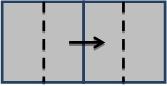
Figure 2. Grid Model

For simplicity, think of the elements outlined by solid lines as cubes of equal size, and that the vector represents a velocity in the x direction. The dashed lines in the centers of the elements (i.e., y-z planes) define the extent of the partial volumes of the elements assigned to the u velocity. The total mass of fluid in the partial volumes correlates to the mass M in the mechanical model. When the velocity U moves fluid between elements the elements respond by generating forces that act to counter the velocity, much like the springs in the mechanical model. These forces may arise because of compression or expansion of the fluid, viscous stresses, surface tension (if there is a fluid interface within the fluid mass M) or other forces. By identifying the appropriate stiffness coefficient k in each case we can use Eq. 5 to arrive at a stability criterion for that physical process when using an explicit numerical approximation in a grid like that shown in Fig. 2.

간단히, 실선에 의해 윤곽이 그려져 있는 요소가 동일 크기의 입방체라고하고 벡터 x 방향의 속도를 나타내는 것으로 생각합니다. 두 요소의 중앙 (즉 yx 평면)의 점선에 의해 속도 U에 할당 된 요소의 부분 체적의 범위가 정의됩니다. 부분 체적 내에 유량의 전체 질량은 기계적 모델의 질량 M과 상관 관계가 있습니다. 속도 U는 응답 요소 사이의 유체가 이동 된 경우 기계적 모델 스프링과 마찬가지로 속도에 대항하여 작용하는 힘을 발생하여 요소는 응답합니다. 이러한 힘은 유체 점성 응력, 표면 장력 (유체와 질량 M의 범위 내에 유체 계면가있는 경우) 또는 기타의 힘에 의한 압축 또는 인장으로 인해 발생 될 수 있습니다. 각 예에서 적절한 강성 계수 k를 특정하여 그림 2와 같은 격자에서 양으로 수치 근사를 사용하는 경우, 식 5를 사용하여이 물리적 과정에 대한 안정성 기준에 도달 가능합니다.

Several examples of how this analogy can be applied are given in the following sections. In each case the mass M of the fluid in the partial volumes is given by,

이 유사성을 어떻게 적용 할 수 있는지에 대한 예는 다음 절에서 설명합니다. 각 예에서 부분 부피의 유체의 질량 M은 아래 식에 의해 주어집니다.

(6) $\displaystyle M=\rho \delta x\delta y\delta z,$

where ρ is the density of the fluid and elements have dimensions δx, δy and δz.

여기서, ρ는 유체의 밀도이며, 요소의 치수는 δx, δy와 δz입니다.

Compressible Fluids

To find the stiffness coefficient, k, recall that k is a measure of the force generated to resist an applied perturbation. For a compressible fluid this force is related to the change in fluid pressure because of a change in fluid density according to the thermodynamic relation dp=c²dρ, where c is the speed of sound in the fluid. The fluid mass moved across the boundary between the elements is ρUδt*δyδz and the change in density in the element receiving the mass is this mass change divided by the volume of the element, dρ=ρUδt/(δx). The corresponding change in element pressure is then given by

강성 계수 k를 요구하려면, k가 더해진 섭동에 저항하기 위해 만들어지는 힘의 척도임을 기억하십시오. 압축성 유체의 경우,이 힘은 유체 압력의 변화와 관련이 있습니다. 이것은 열역학적 관계 dp = c 2 dρ 의한 유체 밀도의 변화에 의한 것입니다. 여기서 c는 유체의 음속입니다. 요소 사이의 경계를 넘어 이동 한 유체의 질량은 ρUδt * δyδz이며, 질량을받는 요소에서의 밀도 변화는이 질량을 요소의 부피로 나눈 dρ = ρUδt / (δx)입니다. 그 결과, 요소 압력의 대응하는 변화는 아래에 제공됩니다.

(7) $\displaystyle dp={{c}^{2}}d\rho =\frac{\rho {{c}^{2}}U\delta t}{\delta x}.$

The force responding to the U velocity perturbation in each element is the product of the pressure change from Eq. 7 and the cross sectional area of the element δyδz. The effective stiffness of an element k, is therefore the force divided by the initial displacement Uδt,

각 요소의 속도 U의 섭동에 응답하는 힘은 식 7에 의한 압력 변화와 요소 단면적 δyδz의 곱입니다. 따라서 요소의 유효 강성 k는 힘을 초기 변위 Uδt로 나눈 것입니다.

(8) $\displaystyle k=\frac{\rho {{c}^{2}}U\delta t\delta y\delta z}{\delta xU\delta t}=\frac{\rho {{c}^{2}}\delta y\delta z}{\delta x}$

Substituting this value for k and the definition for M, from Eq. 6, into the stability condition Eq. 5 results in the stability condition for compressible fluids,

이 k의 값과 식 6에 따르면 M의 정의를 안정성 조건 식 5에 대입하여 압축성 유체의 안정성 조건을 얻을 수 있습니다.

(9) $\displaystyle \frac{k\delta {{t}^{2}}}{M}={{\left( \frac{c\delta t}{\delta x} \right)}^{2}}\le 1.$

This is the well-known Courant condition than restricts the distance a sound wave travels in one time step to be less than the width of a computational element. An analogy with the simple mechanical model has provided this result without the need to write out an equation for pressure waves in a compressible fluid and then perform a stability analysis on that equation.

이것은 하나의 시간 스텝 중에 음파가 진행하는 거리를 계산 요소의 폭보다 짧게 제한하는 잘 알려진 쿨랑 조건입니다. 간단한 기계적 모델과의 유사성에 따라 압축성 유체 음파 방정식을 기술하고, 그 방정식에 의한 안정성 분석을 수행 할 필요없이이 결과를 얻을 수 있었습니다.

Viscous Stresses / 점성 응력

The viscous forces that are generated in response to a perturbed velocity U in a fluid of viscosity μ consist of shears in the x, y and z directions. For example, the shear stress on the lower surface of the element for the velocity U is μU/δz, assuming that the velocity in neighboring cells is zero. There is a corresponding stress at the upper surface of the element. Each of these stresses act on a surface of area δxδy (in the current example) to produce a viscous force. Similarly, there are stresses in the x and y direction acting on their corresponding areas. In each direction there are force pairs (similar to the two springs) but because of Eq. 5 it is necessary to use the effective k for a single spring. This is half of the total of all the the viscous forces divided by the initial displacement Uδt,

점도 μ의 유체의 섭동 속도 U에 대해 생성되는 점성 힘은 x, y 및 z 방향의 전단력으로 구성됩니다. 예를 들어, 인접 셀의 속도가 0이라고 가정하면 속도 U에 요소의 아랫면에 작용하는 전단 응력은 μU / δz입니다. 요소의 표면에는 압축 응력이 발생합니다. 이러한 응력의 각각은 표면적 δxδy (본 예의 경우)에 작용하고 점성 힘을 발생합니다. 마찬가지로 해당 면적에 작용하는 x 및 y 방향의 응력도 존재합니다. 각 방향에서 (2 개의 봄처럼) 세트 힘이 존재하지만, 식 5를 위해 1 개의 봄의 유효 강성 k를 사용하는 것이 필요합니다. 이것은 모든 점성 힘의 합계를 초기 변위 Uδt로 나눈 것의 절반입니다.

(10) $\displaystyle k=\mu \left( \frac{U\delta y\delta z}{\delta x}+\frac{U\delta x\delta z}{\delta y}+\frac{U\delta x\delta y}{\delta z} \right)\frac{1}{U\delta t}.$

Inserting this value for k and using Eq. 6 for M into the stability condition for the mechanical model given in Eq. 5 yields

식 5에 의해 주어진 기계적 모델의 안정 조건에 k의 값을 넣고 M 식 6을 사용하면 아래 식을 얻을 수 있습니다.

(11) $\displaystyle \frac{k\delta {{t}^{2}}}{M}=\frac{\mu }{\rho }\left( \frac{1}{\delta {{x}^{2}}}+\frac{1}{\delta {{y}^{2}}}+\frac{1}{\delta {{z}^{2}}} \right)\delta t\le 1.$

Equation 11 is the stability condition for explicit viscous stresses approximated in an Eulerian grid.

식 11은 오일러 격자에 근접한 explicit 점성 응력의 안정성 조건입니다.

Surface Tension

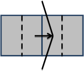
Figure 2A. With deformed interface.

Imagine a fluid interface located between the two elements that is deformed by a U velocity perturbation, as shown in Fig. 2A. In this case the reaction is a surface tension force on each of the segments of the surface illustrated in Fig. 2A. For simplicity, assume a two-dimensional surface (e.g., no variation in the z direction) and a constant surface tension coefficient σ.

그림 2A와 같이 속도 섭동 U에 의해 변형된 2 개의 요소 사이에 위치하는 유체 계면을 상정합니다. 이 예에서, 반응은 그림 2A에 표시된 표면의 각 구분에 작용하는 표면 장력에 의한 힘입니다. 간단히 2 차원 표면 (예 : z 방향의 변화없이)과 일정한 표면 장력 계수를 가정합니다.

Surface tension in each segment acts tangentially along the surface so the force responding to the U velocity is the x component of that force, i.e., the surface tension coefficient times the sine of the angle of the surface segment with respect to the vertical. For a small initial displacement, the x-force from each surface segment can be approximated by σUδtδz/δy giving the resulting stiffness coefficient,

각 구분의 표면 장력은 표면에 따라서 접선 방향으로 작용하기 때문에 속도 U에 대응하는 힘은 표면 장력의 x 성분입니다. 즉, 수직의 표면 구분 각도의 사인을 표면 장력에 곱한 것입니다. 작은 초기 변위의 경우 각 표면 세그먼트에서 x 방향의 힘은 σUδtδz / δy 의해 근사 할 수 있으며, 그 결과로 다음의 강성 계수를 얻을 수 있습니다.

(12) $\displaystyle k=\left( \frac{\sigma U\delta t\delta z}{\delta y} \right)\frac{1}{U\delta t}$

Substituting this k and M into Eq. 5 gives the stability condition for surface tension,

이 k와 M을 식 5에 대입하면 표면 장력에 대한 안정성 조건을 얻을 수 있습니다.

(13) $\displaystyle \frac{k\delta {{t}^{2}}}{M}=\frac{\sigma }{\rho }\frac{\delta {{t}^{2}}}{\delta x\delta {{y}^{2}}}\le 1.$

This result appears somewhat odd because of the different exponents of the δx and δy factors, but for cubic or square elements this makes no difference. For non-uniform elements, however, we should perform a similar evaluation in the y and z directions and then use the most restrictive of the results. In any case, this is a reasonable and useful result from a very simple model based on action and reaction principles.

이 결과는 δx과 δy 지수가 다르기 때문에 다소 이상하게 보이지만, 입방체 또는 사각형 요소의 경우 그 영향은 없습니다. 하지만 For non-uniform 요소의 경우 y 및 z 방향에서 비슷한 평가를 실시하여 가장 제한적인 결과를 사용할 수 있어야합니다. 어쨌든, 이것은 작용과 반작용의 원리에 근거한 매우 간단한 모델에 의한 합리적이고 유익한 결과입니다.

Bulk Elasticity / 체적 탄성

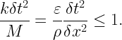
For a fluid with elastic properties the U velocity perturbation is resisted by an elastic stress in a way that closely resembles a spring. If ε is the bulk modulus of the fluid then the stress associated with extension or compression in an element is εUδt/δx. This stress acts over the surface area δyδz, and the stiffness k is this force divided by the displacement Uδt. Substituting this into Eq. 5 provides the stability condition,

탄성 특성을 가진 유체의 경우 속도 U의 섭동은 스프링과 잘 닮은 형식의 탄성 응력에 의해 제한됩니다. 유체의 체적 탄성률이 ε의 경우 요소의 인장 또는 압축에 관련하는 응력은 εUδt / δx입니다. 이 응력은 표면적 δyδz 작용하고 강성 k는이 힘을 변위 Uδt로 나눈 것입니다. 이것을 식 5에 대입하면 아래의 안정성 조건을 얻을 수 있습니다.

(14) $\displaystyle \frac{k\delta {{t}^{2}}}{M}=\frac{\varepsilon }{\rho }\frac{\delta {{t}^{2}}}{\delta {{x}^{2}}}\le 1.$

Similar results exist for the y and z directions.

비슷한 결과가 y 및 z 방향으로도 존재합니다.

Concluding Remarks

A simple mechanical model has been used to illustrate a common type of numerical instability, that arises from an action-reaction process. Using this simple model it is possible to quickly derive a variety of stability conditions for fluid dynamic forces modeled by explicit finite difference approximations in an Eulerian grid. The stability conditions are derived by using mass and force concepts in fluids that are analogous to the mass and forces in the model mechanical system. Significantly, the stability conditions arrived at are generic and do not depend on specific finite-difference approximations. Additionally, these derivations provide a simple way to understand the mechanisms driving the unstable behavior.

간단한 기계적 모델을 사용하여 작용과 반응 과정에서 발생하는 일반적인 유형의 수치 불안정성에 대해 설명했습니다. 이 간단한 모델을 사용하여 오일러 격자의 양으로 유한 차분 근사에 의해 모델링 된 유체 역학적인 힘에 대한 다양한 안정성 조건을 신속하게 도출 할 수 있습니다. 이러한 안정성 조건은 기계적 모델 시스템의 질량과 힘 유사한 유체의 질량과 힘의 개념을 이용하여 도출됩니다. 중요한 점은 도달한 안정성 조건이 일반적이며 특정 유한 차분 근사에 의존하지 않는 것입니다. 또한이 도출에 의해 불안정한 거동을 야기 메커니즘을 이해하는 간단한 방법도 제공됩니다.

The approach taken here could be extended to other types of physical forces (e.g., electrical, non-inertial, etc.) and even advective processes could be included by using the analogy that a change in momentum resulting from advection could be thought of as the result of an equivalent force.

여기서 사용한 방법은 다른 유형의 물리적 힘 (예 : 전기적 힘 비 관성력 등)로 확장 할 수 있으며, 이류(advective )에 의해 생기는 운동량의 변화를 등가 힘의 결과로 생각되면 유사성을 이용함으로써 이류 과정조차 포함 할 수 있습니다.

Furthermore, more refined estimates of the stiffness coefficient, for instance, by including more dimensional effects, could be added to enhance the stability conditions. In any case, the object here is to show that numerical instabilities can often be understood from a simple analysis. It is hoped that the insight this provides might guide the development of more robust and accurate numerical approximations.

또한, 예를 들어 더 많은 차원 효과를 포함하여 강성 계수보다 정밀한 추정을 추가하고 안정성 조건을 강화 할 수 있습니다. 어쨌든 여기에서의 목표는 대부분의 경우 수치 불안정성을 간단한 분석에서 이해하고 보여주는 것입니다. 여기에 제공된 통찰력이 더 강력하고 정확한 수치 근사치의 개발로 이어질 것으로 기대됩니다.

General CFD

A basic requirement for computational fluid dynamics

전산 유체 역학 (CFD)의 기본 요구 사항은 밀도, 압력 및 속도 등의 유체 특성을 각 요소에 대해 고유하게 할당할 수있는 미소 요소에 공간을 이산화하는 것입니다.

공간을 분할하는 다양한 방법 중 일반적인 방법의 일부는 격자 시스템에 쉽게 설명되어 있으며, 각각의 방법에 대해 장단점도 기술되어 있습니다.

사각형 격자 요소는 아마도 수치 근사를 위해 생성하고 사용하는 가장 간단한 격자 요소이지만, 일반적인 사용이 제한되어 너무 대체로 간주합니다.

사각형 격자는 여러 가지 방법으로 사각형 격자를 쉽게 확장하고 복잡한 격자 생성의 가능성을 제공할 수 있다고 설명하면 위의 생각이 틀렸다는 것을 보여줍니다.

A basic requirement for computational fluid dynamics (CFD) is to have a discretization of space into small elements in which fluid properties such as density, pressure and velocity can be uniquely assigned to each element. There are a variety of ways to subdivide space and some of the more common ones are briefly described in the article Grid Systems, which offers a few pros and cons for each possibility. Rectangular grid elements are probably the simplest to generate and use for numerical approximation, but are often seen as too restricted for general use. The article Rectangular Grids shows the fallacy of this by explaining how rectangular grids can be easily extended in several ways to offer more complex gridding possibilities.

CFD를 실제 문제에 적용하려면, 질량, 운동량 및 에너지 보존에 관한 기본적인 유체 방정식의 단순한 수치 모델 이상의 경우를 고려하는 것이 필요합니다. 이러한 문제의 일부는 아래에 있는 General CFD 절에서 논의되고 있습니다.

자유 유체 표면 또는 액체 계면을 수치적으로 모델링하는 다양한 방법의 개요가 나와 있습니다.

그 밖에도 난류 현상을 모델링하는 방식이 논의되고 있으며, 마지막으로 이산 질량 (또는 마커) 입자의 사용에 대한 일반적인 논의도 포함되어 있습니다.

직관적으로 이산 입자는 복잡한 유체 흐름의 변화을 추적하는데 이상적이라고 생각되지만, 마지막 부분에서 설명된 바와 같이 이산 입자와 관련된 많은 제한에 대해 유의해야 합니다.

Application of CFD to real problems often requires more than a straightforward numerical model of the basic fluid equations for conservation of mass, momentum and energy. Several of these issues are discussed in the remaining articles under the heading of General CFD. A short summary is given of different ways to numerically model free fluid surfaces or fluid interfaces. Another of the articles discusses approaches for modeling turbulence phenomena, and finally, there is a general discussion of the use of discrete mass (or marker) particles. Intuitively, discrete particles would seem to be ideal for tracking the evolution of complex fluid flow, however, as this last article explains, there are a number of limitations associated with discrete particles that should be kept in mind.

이전 페이지

다음 페이지

본 자료는 국내 사용자들의 편의를 위해 원문 번역을 해서 제공하기 때문에 일부 오역이 있을 수 있어서 원문과 함께 수록합니다. 자료를 이용하실 때 참고하시기 바랍니다.

Slot Coating

Slot Die Coating

FLOW-3D는 슬롯 다이 코팅의 산업 연구 및 설계에 사용됩니다. 슬롯 다이 코팅에서 유체는 슬롯에서 슬롯에 매우 가까운 곳에 위치한 빠르게 움직이는 기판 위로 강제 배출됩니다. 때로는 여러 슬롯을 사용하여 여러 재료의 레이어드 코팅을 만들기도 합니다. 많은 산업에서 슬롯 다이 코팅 기계는 상대적으로 단순하기 때문에 슬롯 다이코팅이 사용됩니다. 슬롯 다이 코팅의 또 다른 이점은 나노미터 단위로 측정한 코팅 두께에서도 높은 코팅 균일성 비율입니다.

아래 예에서, 한 슬롯은 120미크론 두께의 뉴턴이 아닌 재료를 오른쪽에서 왼쪽으로 움직이는 기질에 적용하고 있습니다.

FLOW-3D에서 유체-솔리드 접촉 선과 접촉각은 흐름의 전체 역학의 일부로 자동으로 계산됩니다. 이것은 슬롯과 웹(Web) 사이의 영역에서 세 개의 개별 접촉 선이 발생하는이 예에서 잘 설명됩니다.

Case Study

Roche Diagnostics GmbH가 2014년 FLOW-3D 유럽 사용자 컨퍼런스에서 발표한 산업 사례 연구의 이 이미지는 진공 보조 장치가 없는 슬롯 다이 코팅의 3D 모델을 보여줍니다. 왼쪽 상단에 그려진 실험과 FLOW-3D로 수행된 시뮬레이션 사이에는 훌륭하게 일치하고 있습니다.

*Simulation of a slot die coating without vacuum assist, courtesy Roche Diagnostics GmbH*

Slot Die Design

아래에 표시된 3M의 FLOW-3D 시뮬레이션은 슬롯 다이의 내부 캐비티 내부의 유체 체류 시간을 보여줍니다. 슬롯 다이 설계는 코팅 프로세스의 성공에 매우 중요하며 코팅 액의 유변학(rheology)에 따라 다릅니다.

Simulation courtesy of 3M

Two-Layer Slot Coating

왼쪽의 시계열 이미지에서 보면 웹(web)이 이동되고, 슬롯 코팅 다이는 두 개의 슬롯에서 서로 다른 물성의 두 유체가 나오고 있습니다. two-layer slot die를 사용하는 이점은 코팅기의 die station의 수를 감소시킬 수 있는 것입니다. 그러나, 단일 층의 경우에는 존재하지 않는 이층 슬롯 코팅에 존재하는 많은 문제점들이 나타납니다. 두 개의 유체 층 사이의 계면(interface), 보통은 혼합될 수 있는 물성을 가진 Interlayer 는 die surfae에 안정적으로 잘 고정되어야 합니다. 그리고 Interlayer 부근이 순환은 두 유체의 혼합을 막기 위해 최소화 되어야만 합니다. 일반적으로 이것들은 각각의 유체의 밀도, 점도 및 유량이 배출율을 조작함으로써 제어될 수 있습니다.

Start-Up of Slot Coating

슬롯 코터를 이용하여 연속 코팅 공정을 시작하면 시작부터 폐기해야 불완전한 재료의 양을 감소시키기 위해, 가능한 한 빨리 균일한 wettig을 수립하는 것이 바람직합니다. Wet start 기술은 잉크가 웹에 가까워지기 전에 슬롯에서 잘 빠져 나오는 것 보장하는 중요한 기술중의 하나입니다. 이 예에서, web은 액체의 상류 및 하류 모두 압착 슬롯을 향해 이동된다.

슬롯 장치의 경사진 앞쪽면에 유체를 위로 밀어올리는 약간 늦은 적당한 접근 속도는 슬롯장치의 더 나은 성능을 제공합니다.

Slide Coating

모든 코팅 공정은 코팅 물질이 정상 상태에 도달하기 전에 큰 변형을 겪게 되는 초기 전개 시기(startup period)를 가집니다. 초기 전개 시기의 좋은 특성들은 유체의 낭비를 감소시키고 공정을 기술자가 원하는 범위 내에서 작동시키게 합니다.

다층 커튼 코팅 공정의 경우, 아래 시뮬레이션에서 볼 수 있듯이 유체가 슬롯 다이에서 배출된 다음 물질이 중력에 노출 될 수 있습니다.

유체층은 일반적으로 서로 다른 특성을 갖지만 자주 혼합되기 때문에 층 사이의 계면 장력이 작습니다. 특히 중요한 것은 다이면에서 정적 접촉 라인의 위치와 안정성, 그리고 유체가 이동 표면과 처음 만나는 동적 접촉 라인입니다. 이 위치는 유체 흐름 속도, 움직이는 기판의 속도 및 동적 접촉 상류의 공기 공간의 진공 양에 의해 영향을받습니다. 또한 중요한 것은 각 유체 사이에 날카로운 중간층을 유지하는 것입니다. FLOW-3D는 완전히 일시적인 3 차원 흐름 모델이므로 시작하는 동안 프로세스의 일시적인 동작을 시뮬레이션 할 수 있습니다.

*Startup of a multi-layer slide coating*

모든 코팅 공정에는 일정한 조건을 달성하기 전에 코팅 재료가 큰 변형을 겪는 일종의 시작 기간이 포함됩니다. 시작 프로세스의 우수한 특성화는 낭비를 줄이고 프로세스가 원하는 한계 내에서 작동하는지 확인하는 데 중요합니다. 다양한 섭동에 대한 코팅 흐름의 일시적인 반응에 대한 유사한 이해가 또한 바람직하여 코팅 비드의 파손 및 코팅의 불균일성을 방지 할 수 있습니다.

Curtain Coating

커튼 코팅에서 액체는 슬롯이나 슬라이드 다이에서 흘러 나와 중력을 받아 수평으로 움직이는 기판에 떨어집니다. 커튼 코팅은 단일 층의 유체 또는 다중 유체 층을 포함 할 수 있으며 사진 필름, 특수 용지 및 포장의 생산에 사용됩니다.

슬롯에서 나오는 유속과 관련된 액체의 물리적 특성과 기질 속도에 따라 액체가 먼저 기질에 접촉하는 접촉선의 안정성은 물론 코팅 두께를 결정합니다.
접촉 라인이 불안정하면 코팅 아래에 웅덩이나 공기 유입이 발생하여 균일하지 않은 코팅 두께 및 기타 결함을 발생시킬 수 있습니다.
FLOW-3D는 유량, 유량, 기질 속도 등 다양한 공정 파라미터로 공정을 시뮬레이션하고 점성, 표면 장력, 접착력 등 액체의 물리적 성질을 변화시켜 커튼 코팅의 안정성을 조사하는 데 사용할 수 있습니다.

Water Rivers Bridge Piers

Bridge Piers

FLOW-3D의 Sediment Scour Model 은 강이나 하천에서 수리학적으로 복잡한 교각과 지형에 따라 여러가지 퇴적물들의 높이 변화를 해석할 수 있습니다. 세굴 모델은 FLOW-3D 난류 모델들로 적분하여 3차원 분석이 가능합니다. FLOW-3D의 Shallow Water Model로 더 넓은 범위의 세굴 분석이 가능합니다.

교각 주위의 세굴 해석

세굴 모델은 deposition, packing, entrainment and drift-flux 메커니즘으로 되어있습니다. FLOW-3D v11 에서는 퇴적층의 형상을 FAVOR 하여 좀 더 정확하게 bed net 높이 변화를 시각화 할 수 있습니다. 시공간적으로 침전물의 변화뿐 아니라 유체의 부유물들, 바닥/유체 계면에서의 전단응력들을 분석할 수 있습니다.

Modeling Hydraulic Control Structures

In addition to the flow rates and detail of hydraulic behaviors associated with the control gate structures and powerhouse operation, FLOW-3D‘s sediment and scour model allows users to identify regions of high scour both near the control structure and further downstream in the vicinity of the bridge piers.

Bridge Pier Simulations

The first video shows a FLOW-3D simulation of the erosion that occurs around a group of three 2.4 m diameter piers as river water flows past at 1.5 m/s. The river depth is 15.8 m and the mean sediment size was presumed to be 0.35 mm.

Why FLOW-3D?

Why FLOW-3D ?

FLOW-3D는 엔지니어들에게 다양한 분야의 유동해석에 대해 귀중한 통찰력을 제공하는 강력한 모델링 도구입니다. 정확하게 자유 표면 흐름을 예측하는 특별한 기능을 통해 FLOW-3D는 설계 단계에서뿐만 아니라, 생산 공정 개선에도 사용할 수 있는 이상적인 전산 유체 역학 (CFD) 소프트웨어입니다.

TruVOF and Free Surface Modeling

FLOW-3D 는 다른 유동해석 프로그램과는 유체 계면을 다루는 기법이 확연하게 다릅니다. FLOW-3D 는 자유표면의 위치를 추적하고, 그 자유표면에 적절한 동적 경계 조건을 적용하는 특수한 수치기법(numerical method)을 사용합니다. FLOW-3D 에서 모델링된 자유표면은 로스알라모스 국립 연구소에서 Flow Science의 설립자인 C. W. Hirt 박사와 함께 소속한 과학자 그룹에 의해서 개발된 VOF(Volume of Fluid) 기법으로 모델링됩니다. CFD 프로그램의 대부분은 세 가지 기본 VOF 성분 중 실제로는 단지 하나 또는 두 가지만 구현하여 VOF 기능을 통합 구현한 것으로 주장하고 있습니다. CFD 사용자는 이러한 유사 VOF 기법으론 종종 잘못된 결과를 얻을 수 있음을 알고 있어야 합니다. FLOW-3D는 자유표면의 성공적인 해석에 필요한 모든 요소를 포함하고 있습니다. 또한, FLOW-3D는 경계 조건과 계면 추적의 정확도를 증가시키기 위해 원래의 VOF 방법을 크게 향상 시키고 있습니다. 좀더 자세한 사항은 TruVOF 방법을 참고하시기 바랍니다.

<CFD-101에 FLOW-3D의 TruVOF 방법에 대해 자세히 알아보기>

Free Gridding Separates Meshing from Geometry Construction

Gridding에 대한 FLOW-3D’의 기본 접근 방식은 deformed, body-fitted grids의 유연성과 단순한 직사각형 그리드의 장점을 결합합니다. 직사각형 컨트롤 요소의 고정 그리드는 간단하고 매우 바람직한 특성을 갖도록(예를 들어, 향상된 정확도, 작은 메모리 크기 요구, 간단한 수치 근사치) 생성 처리됩니다. 이 접근법은 그리드나 형상을 각각 서로 독립적으로 자유롭게 변경 할 수 있기 때문에 “free-gridding”으로 지칭합니다.

이 기능은 body-fitted 또는 유한 요소 격자를 생성하는 지루한 작업을 하지 않도록 해 줍니다.

Rectangular gridding 의 유연성과 효율은 multi-block 과 conforming meshing 같은 고급 기능에 의해 강화됩니다. 연결되어 있고 부분적으로 중첩된 메쉬 블록은 복잡한 멀티 스케일 유동 도메인과 관심 영역에서 효과적으로 높은 해상도를 가질 수 있는 수단을 제공합니다. Conforming mesh는 직사각형 gridding 구조와 관계 없이 특별한 기하학적 형상, cavities, 얇은 구조물, 경계층 등에 적합한 고품질의 grids를 생성할 수 있습니다.

Modeling Fluid Flow in Complex Geometry is Easy with FAVOR™

FLOW-3D 는 직사각형 격자 내에서 일반 기하학적 영역을 정의하는데 사용되는 FAVOR™ (Fractional Area Volume Obstacle Representation) 방법으로 알려진 특별한 기술을 사용합니다. FAVOR™ 기본 철학은 수치 알고리즘이 각 제어 체적(control volume)에 대해 하나의 압력, 하나의 속도, 하나의 온도 등으로 이루어지는 정보를 기반으로 하므로 형상을 정의하는 데 많은 정보를 사용하는 것이 적합하지 않는다는 것입니다. 따라서, FAVOR ™ 기술은 직사각형 격자의 단순성을 유지하면서 각 제어 체적 내의 유동 값의 정밀도와 일치하는 수준으로 복잡한 기하학적 형상을 나타냅니다.

Meshing Capabilities

FLOW-3D 는 복잡한 유체 해석 모델링시 간단하면서도 효율적이고 견고한 대규모 격자 생성 능력을 제공합니다. 특히, FLOW-3D의 효율좋은 단순한 메쉬 구조와 다중 블록 메쉬의 다양한 특징에 의해 최고의 메싱 효율과 견고성을 자랑합니다. 여러개의 메쉬 블록 사용은 관심 영역의 최적화를 허용하고 주어진 시뮬레이션에 필요한 연산 리소스를 훨씬 감소시킵니다. 작은 장애물(Small obstacles), 복잡한 형상 그리고 전체 영역 크기에 비해 좁은 통로(channel)는 다음과 같은 linked, nested, conforming, 그리고/또는 부분 중첩 mesh blocks등의 여러 다중 블록 메싱능력 중 하나를 사용하여 정확히 해결 될 수있습니다. Linked mesh blocks은 관심영역의 격자 생성과 계산 격자의 총 수를 제한하는 데에만 사용될 수 있습니다. Nested mesh blocks은 관심영역 주위의 해상도를 향상시키기 위해 사용될 수 있습니다. Conforming 과 partially overlapping mesh blocks은 단순히 중첩된 급격한 변화와 불규칙한 형상을 해결하기 위해사용될 수 있습니다. FLOW-3D 는 또한 Fluid-Structure Interaction에 필요한 body-fitted 유한요소 격자를 허용합니다. 이 body-fitted 격자는 FLOW-3D 또는 외부 CAD 패키지 S/W로 부터 가져와 자동으로 생성할 수 있습니다. 이 모든 메쉬 기술은 사용자에게 간단하면서 효율적으로 메쉬를 생성하게 하여 솔버 성능 향상 및 해석시간을 줄이는 유연성을 제공합니다.

: Linked meshes

: Conforming mesh

: Nested mesh block

: Partially-overlapping mesh

Tag: 계면