A basic requirement for computational fluid dynamics
전산 유체 역학 (CFD)의 기본 요구 사항은 밀도, 압력 및 속도 등의 유체 특성을 각 요소에 대해 고유하게 할당할 수있는 미소 요소에 공간을 이산화하는 것입니다.
공간을 분할하는 다양한 방법 중 일반적인 방법의 일부는 격자 시스템에 쉽게 설명되어 있으며, 각각의 방법에 대해 장단점도 기술되어 있습니다.
사각형 격자 요소는 아마도 수치 근사를 위해 생성하고 사용하는 가장 간단한 격자 요소이지만, 일반적인 사용이 제한되어 너무 대체로 간주합니다.
사각형 격자는 여러 가지 방법으로 사각형 격자를 쉽게 확장하고 복잡한 격자 생성의 가능성을 제공할 수 있다고 설명하면 위의 생각이 틀렸다는 것을 보여줍니다.
A basic requirement for computational fluid dynamics (CFD) is to have a discretization of space into small elements in which fluid properties such as density, pressure and velocity can be uniquely assigned to each element. There are a variety of ways to subdivide space and some of the more common ones are briefly described in the article Grid Systems, which offers a few pros and cons for each possibility. Rectangular grid elements are probably the simplest to generate and use for numerical approximation, but are often seen as too restricted for general use. The article Rectangular Grids shows the fallacy of this by explaining how rectangular grids can be easily extended in several ways to offer more complex gridding possibilities.
CFD를 실제 문제에 적용하려면, 질량, 운동량 및 에너지 보존에 관한 기본적인 유체 방정식의 단순한 수치 모델 이상의 경우를 고려하는 것이 필요합니다. 이러한 문제의 일부는 아래에 있는 General CFD 절에서 논의되고 있습니다.
자유 유체 표면 또는 액체 계면을 수치적으로 모델링하는 다양한 방법의 개요가 나와 있습니다.
그 밖에도 난류 현상을 모델링하는 방식이 논의되고 있으며, 마지막으로 이산 질량 (또는 마커) 입자의 사용에 대한 일반적인 논의도 포함되어 있습니다.
직관적으로 이산 입자는 복잡한 유체 흐름의 변화을 추적하는데 이상적이라고 생각되지만, 마지막 부분에서 설명된 바와 같이 이산 입자와 관련된 많은 제한에 대해 유의해야 합니다.
Application of CFD to real problems often requires more than a straightforward numerical model of the basic fluid equations for conservation of mass, momentum and energy. Several of these issues are discussed in the remaining articles under the heading of General CFD. A short summary is given of different ways to numerically model free fluid surfaces or fluid interfaces. Another of the articles discusses approaches for modeling turbulence phenomena, and finally, there is a general discussion of the use of discrete mass (or marker) particles. Intuitively, discrete particles would seem to be ideal for tracking the evolution of complex fluid flow, however, as this last article explains, there are a number of limitations associated with discrete particles that should be kept in mind.
유체 흐름 문제는 복잡한 기하학적 구조의 자유 표면과 관련되는 경우가 많으며 대부분 매우 일시적입니다. 수력학의 예로는 배수로, 강, 교각 주변, 홍수 범람, 수문, 잠금 장치 및 다수의 기타 구조물의 흐름이 있습니다. 이러한 유형의 흐름을 계산적으로 모델링 하는 능력은 이러한 계산이 정확하고 합리적인 계산 자원으로 수행될 수 있다면 매력적입니다. 유용하게 사용하려면 시뮬레이션은 물리적 모델을 사용하는 것보다 훨씬 빠르고 저렴해야 합니다.
Fluid flow problems often involve free surfaces in complex geometry and in many cases are highly transient. Examples in hydraulics are flows over spillways, in rivers, around bridge pilings, flood overflows, flows in sluices, locks, and a host of other structures. A capability to computationally model these types of flows is attractive if such computations can be done accurately and with reasonable computational resources. To be useful, simulations should be much faster and less expensive than using physical models.
많은 컴퓨터 프로그램은 유체의 역학을 설명하는 편미분 방정식을 풀 수 있습니다. 시뮬레이션에 자유 표면을 포함 할 수있는 프로그램은 많지 않습니다. 그 이유는 Free Surface 경계 문제로 잘 알려진 수학적인 문제입니다. 자유 경계 문제는 다루기 어려운 표면이 이동함에 따라 계산 영역이 변화하는 한편, 그 표면 이동 자체가 계산에 의해 결정된다는 점에 있습니다. 계산 영역의 변화는 그 크기와 모양의 변화뿐만 아니라, 경우에 따라서는 영역의 결합과 분리(즉, 자유 표면의 발생과 소멸)을 포함합니다.
Many computer programs can solve the partial differential equations describing the dynamics of fluids. Not many programs are capable of including free surfaces in their simulations. The difficulty is a classical mathematical one often referred to as the free-boundary problem. A free boundary poses the difficulty that on the one hand the solution region changes when its surface moves, and on the other hand, the motion of the surface is in turn determined by the solution. Changes in the solution region include not only changes in size and shape, but in some cases, may also include the coalescence and break up of regions (i.e., the loss and gain of free surfaces).
이 책에서는 모든 자유 표면을 고려한 유체흐름 현상을 수치 해석용으로 모델링하는 방법에 대해 설명합니다. 이 기술은 VOF (Volume-of-Fluid) 법에 근거한 것으로, 특히 자유 표면 흐름에 적합한 다양한 기능을 제공합니다. 이 책에서는 VOF 법이 자유 표면과 그 발생과 소멸을 해석하는데 가장 자연스럽고 매우 효율적인 방법을 제시합니다.
In this note a computational modeling technique for fluid flows with arbitrary free surfaces is discussed. The technique is based on the Volume-of-Fluid (VOF) technique. This technique has many unique properties that make it especially applicable to flows having free surfaces. The goal of this discussion is to show why the VOF approach offers a natural way to capture free surfaces and their evolution with great efficiency.
VOF 법의 특징을 잘 보여주기 위해 간단하지만 매우 중요한 유동 현상에 관한 문제를 다룹니다. 여기에서는 계단 낙차형상의 낙하류를 예로 들어 있습니다. 개념적으로 간단한 흐름인 동시에 결과의 타당성을 확인하기위한 좋은 실험 데이터도 제공되어 있습니다 (N. Rajaratnam and MR Chamani “Energy Loss at Drops”J. Hydraulic Res. Vol. 33 p.373,1995 참조).
A good recommendation for the VOF method is to demonstrate its capabilities on a simple hydraulic flow problem, one that is far from trivial. The example selected is of flow over a step. This flow has conceptual simplicity and good experimental data available for validation (see N. Rajaratnam and M.R. Chamani, “Energy Loss at Drops,” J. Hydraulic Res. Vol. 33, p.373, 1995).
Prototype Hydraulic Flow with Free Surfaces
그림 1a는 정상 상태에 도달 한 후 흐름의 문제를 보여줍니다. 계단 낙차형상 상부로부터의 월류(액체 또는 스냅 시트)에는 상하 모두의 자유 표면이 있습니다. 월류의 아래쪽에는 월류와 계단 가공면 사이에 웅덩이가 형성되어 있으며, 하류에서는 액체는 평평한 정상 표면에서 오른쪽으로 흐르고 있습니다. 엄밀히 말하면, 웅덩이 영역의 흐름 상태는 정상입니다. 이것은 충돌하는 액체에 의해 풀에 난류 혼합이 발생하고 있기 때문입니다. 그러나 평균적인 구성이 존재하고 그것은 실험에서도 보고됩니다.
Figure 1a shows the flow problem after it has reached a steady-state condition. The overflow (sheet of liquid or nappe) leaving the top of the step has both an upper and lower free surface. At the bottom of the overflow a pool has formed between the overflow and the face of the step, while downstream, liquid is flowing to the right with a flat, steady surface. Strictly speaking, the flow conditions in the pool region are not steady because turbulent mixing is generated in the pool by the impinging fluid. There is, however, an average configuration and that is what is reported in the experiments.
실용적인 목적 유동 흐름은 항상 2 차원입니다. 즉, 그림 1a에서 수직 방향에서는 큰 변화는 없습니다. 현실에서는 웅덩이 위쪽으로 공간을 만들기 위해서는 대기에 여유공간이 필요하고, 그게 없으면 닫힐 것입니다.
For all practical purposes the flow is two-dimensional, that is, it does not have any significant variation in the direction normal to the illustration in Fig. 1a. In actuality, to have an air space above the pool there must be some opening to the atmosphere otherwise it would close up.
계단 낙차형상 상단의 유속은 중요합니다. 즉, 이것은 표면파와 같거나 그 이상의 속도이기 때문에 하류에서의 교란이 영역을 관통하고 상류 흐름 (계단 낙차형상의 왼쪽)에 영향을 줄 수 없습니다. 따라서 이 영역에서의 흐름은 예외적으로 원활하고 정상입니다.
The flow speed at the top of the step is critical, that is, it has a speed equal to or greater than the speed of surface waves, so that no disturbances from downstream can penetrate through this region to affect flow upstream (to the left of the step), which is why the flow is exceptionally smooth and steady in that region.
이 문제는 수치 시뮬레이션과 비교할 수 있는 기하 형상 기능이 많이 있습니다. 예를 들어, 계단 낙차형상의 전후 흐름의 높이, 월류가 바닥에 충돌 할 때의 각도, 월류 아래에 형성되는 웅덩이의 깊이 등입니다. 또한 실용화를 위한 중요한 비교 항목으로는, 계단 낙차형상을 통해 떨어지는 낙하 류에 의해 손실되는 에너지의 양 (운동 에너지와 위치 에너지의 합)가 있습니다.
There are many geometric features in this problem that can be compared with a numerical simulation; such as flow heights before and after the step, the angle of the overflow stream when it strikes the bottom and the depth of the pool formed under the overflow. Additionally, an important comparison for practical applications is the amount of energy (i.e., kinetic plus potential) lost by the flow in passing over the step.
Simulation of Prototype Problem
그림 1a는 시뮬레이션의 결과입니다. 이 예에서는 실험에 사용된 모든 기하 형상 및 물질의 특성이 시뮬레이션에 사용되었습니다. 실험실 테스트에서 사용한 계단 낙차형상의 높이가 62cm에서 액체는 보통의 물 (밀도 = 1.0gm / cc 어떻게 점성 = 0.01dynes / cm)입니다. 계산 영역에 들어가는 물의 깊이는 15.5cm에서 속도가 임계에 가까운 123.0cm/s 였습니다. 물론, 중력은 수직 방향으로 크기는 g = -980cm / s^2입니다.
Figure 1a is from a simulation. For this example all of the geometric and material properties used in the experiments were used in the simulation. The height of the step used in the laboratory test is 62cm and the fluid is ordinary water (density=1.0 gm/cc and dynamic viscosity=0.01dynes/cm). The depth of water entering the computational region was 15.5cm and was given a near critical velocity of 123.0cm/s. Of course, gravity was in the vertical direction with magnitude g=-980cm/s^2.
Figure 1a. Simulation of flow over a step.
Figure 1b. Grid used in simulation.
월류 왼쪽에 있는 웅덩이에 난류가 발생 할 것으로 예상 되었기 때문에, 시뮬레이션에서는 난류 모델 (the Renormalization Group, 즉 RNG 모델)을 사용했습니다. 그 후, 난류 모델을 사용하지 않고 한 시뮬레이션에서도 비슷한 결과를 얻을 수 있었지만, 이것은 그다지 놀라운 일이 아닙니다. 흐름의 중요한 요소의 대부분은 매끄러운 (즉 난류가 아닌) 유입, 유출, 월류 때문입니다.
Because some turbulence was expected to develop in the pool to the left of the overflow, a turbulence model (the Renormalization Group or RNG model) was used in the simulation. Subsequent simulations without a turbulence model produced very similar results, which is not too surprising since most of the important elements of the flow are smooth (i.e., non-turbulent) inflow, overflow and outflow streams.
그림 1b 시뮬레이션 영역은 폭 170cm, 높이 100cm에 가로 80 개, 세로 60 개, 총 4800 개의 셀로 구성되는 같은 크기의 사각형 셀의 격자로 세분화되어 있습니다. 이 격자는 유체 역학의 지배 미분 방정식 (나비에 – 스토크스 방정식)의 유한 차분 근사의 기초로 사용됩니다. 격자 셀의 수와 크기는 흐름 속에서 예측되는 최소의 특성을 파악하는 목적으로 선택되었습니다. 결과를보고 어떤 조정이 필요하다고 생각되는 경우는 숫자를 쉽게 늘리거나 줄일 수 있습니다. 사실, 해상도를 바꾸어 시뮬레이션을 반복하여 계산이 그러한 변화에 영향을 많이 들어 있지 않은지 확인하는 것이 좋습니다.
The simulation region shown in Fig. 1b is 170cm wide and 100cm high and has been subdivided into a grid of equal sized rectangular cells consisting of 80 cells in the horizontal direction and 60 cells in the vertical direction, for a total of 4800 cells. This grid is used as the basis for finite-difference approximations of the governing differential equations of fluid dynamics (the Navier-Stokes equations). The number and size of the grid cells was chosen with the goal of capturing the smallest expected features of the flow. The number can be easily increased or decreased if the results seem to warrant some adjustment. In fact, it is often a good idea to repeat a simulation with a change of resolution to make sure that the solution is not too sensitive to such changes.
왼쪽의 경계는 지정된 속도 경계입니다 (유체의 높이도 지정). 오른쪽의 경계는 유출 경계에서 모든 유량이 경계에 수직 제로 기울기이며, 균일 한 유출이 촉진됩니다. 상하 경계는 단단한 벽으로 세 번째 방향의 경계는 대칭면 (점성 저항 제로의 벽)으로 처리되었습니다. 계단 낙차형상의 표면도 자유-미끄럼(free slip) 경계로 처리되었습니다.
The left boundary was a specified velocity boundary (also with a specified fluid height). The right boundary was an outflow boundary where all flow quantities have a zero gradient normal to the boundary to encourage a uniform outflow. The top and bottom boundaries are rigid walls, while in the third direction the boundaries were treated as planes of symmetry (i.e., walls with zero viscous drag). The surface of the step was also treated as a free-slip boundary.
초기 조건은 예측되는 흐름의 배열을 대략적으로 근사하도록 설정할 수 있었지만, 흐름의 구성은 계산하고 싶은 것 중 하나이기 때문에 유체가 어떻게 분포되는지를 모르는 경우에는 간단한 방법이 필요합니다. 이 예제에서는 비정상 흐름 시뮬레이터를 사용했기 때문에 그림 1a의 계단 낙차형상에 유체의 블록만 있고 왼쪽 경계의 같은 수평 속도와 높이가 할당된 간단한 초기 조건을 정의할 수 있습니다. 시뮬레이션은 이후 정상 흐름으로 발전하고 있지만, 이것은 약 8.0 초 후에 발생합니다. 시뮬레이션은 정상 상태에 도달 한 것을 보장하기 위해, 10.0 초의 시간까지 실행되었습니다. 그림 2는 중간 시간을 두 보여줍니다. 도 2b는 0.2 초, 그림 2c는 0.5 초 시점에서 그림 2d는 마지막 10.0 초 시점을 보여줍니다.
Initial conditions could have been set to roughly approximate the expected flow arrangement, but since the flow configuration is one of the things that one would like to compute, especially for situations where one doesn’t know what the distribution of fluid is likely to be, a simpler approach is needed. Because a transient flow simulator was used for this example a simple initial condition could be defined that consisted of just a block of fluid on top of the step, Fig. 1a with the same horizontal velocity and height assigned to the left boundary. The simulation then followed the development of the steady flow, which occurs after about 8.0s. The simulation was run out to a time of 10.0s to assure that steady conditions had been reached. Figure 2 shows two intermediate times; 2.b at 0.2s and 2.c at 0.5s plus the final time in 2.d at 10.0s.
Figures 2a-2d. Simulation times of 0.0, 0.2, 0.5 and 10.0s.
처음에는 단일 결합하고 있는 자유 표면이었던 것이 액체가 바닥에 충돌한 후 2 개의 독립적인 자유 표면 (상하 스냅 표면)으로 변화하는 것에 주목하십시오. 아래 경계의 충격점의 좌우로 흐름이 분리되도 문제는 없습니다. 이에 대해서는 다음 섹션에서 자세히 설명합니다.
It should be noted that what starts as a single, connected free surface changes to two independent free surfaces (upper and lower nappe surfaces) after the fluid strikes the bottom. No difficulties are experienced with this separation of the flow into portions flowing to the left and right of the impact point on the bottom boundary. This will be discussed at further length in the next section.
실험과 시뮬레이션의 비교는 다음 표와 같으며 매우 잘 일치하고 있습니다.
Comparisons between experiment and simulation are given in the following table and are in excellent agreement.
Comparison Table
Experimental Results
Simulation Results
Outflow Height/Step Height
0.094
0.094
Pool Height/Step Height
0.41
0.41
Angle of Nappe at Bottom
57°
59°
Energy Loss/Initial Energy
0.29
0.296
이러한 결과를 고려하면이 같은 정밀도를 달성하려면 상당한 계산시간이 필요할 것으로 생각될지도 모릅니다. 그러나 실제로는 Pentium 4, 3.20GHz의 데스크톱 컴퓨터의 총 CPU 시간은 단 88 초였습니다. 계산시간이 너무 짧은 것은 설명이 필요하며, 이것은 다음 섹션의 목적입니다.
In view of these results it might be expected that a considerable amount of computational time would be required to achieve such accuracy. In fact, the total cpu time on a desktop Pentium 4, 3.20GHz computer was only 88s. Such a short computational time requires explanation and that is the purpose of the following sections.
Figures 2a-2d. Simulation times of 0.0, 0.2, 0.5 and 10.0s.
Why the VOF Technique Works Well / VOF 법이 적합한 이유
VOF 법의 구조와 그것이 매우 효율적인 방법인 이유를 이해하기 위해 다양한 계산법 중에서도 특히 VOF 법에 대한 몇 가지 기본 개념을 나타냅니다.
There are a few general concepts about computational methods and the VOF technique in particular that can be used to gain an understanding of how and why VOF works so efficiently.
Basic Theory
모든 수치해석 방법에서 흐름의 문제를 단순하게 산술 계산하도록 유한의 수치 세트로 단순화해야합니다. 연속 유체를 이산화된 수치 세트에 근사하기 위해서 일반적으로 사용되는 것이 유체가 차지하는 공간을 격자로 분할하는 방법입니다. 이 격자는 일반적으로 다수의 작은 직사각형의 블록(요소)로 구성됩니다. 이러한 각 요소에 대해 평균화 처리를 실시함으로써 그 요소의 유체의 압력, 밀도, 속도 및 온도의 대표 값을 얻을 수 있습니다.
All numerical methods must use some simplification to reduce a fluid flow problem to a finite set of numerical values that can then be manipulated using elementary arithmetical operations. A typical procedure for approximating a continuous fluid by a discrete set of numerical values is to subdivide the space occupied by the fluid into a grid consisting of a set of small, often rectangular “bricks.” Within each element an averaging process is applied to obtain representative element values for the fluid’s pressure, density, velocity and temperature.
간단한 수식을 사용해, 어느 시간에 걸친 각 요소 값과 인접한 요소의 상호 작용을 근사할 수 있습니다. 예를 들어, 요소의 밀도는 그 요소와 인접 요소 사이에서 (질량 보존에 의한) 질량 유량이 교환된 경우에만 변경됩니다. 요소 사이에서 질량이 교환되는 물질의 속도는 운동량 보존 법칙에 의해 계산되며 일반적으로 나비에-스토크스 방정식으로 표현됩니다. 나비에-스토크스 방정식은 인접한 요소 사이에 작용하는 압력과 점성 응력을 이용하여 요소에서 변화하는 유체 속도를 근사합니다.
Simple equations can be devised to approximate how each element’s values interact with neighboring elements over time. For instance, the density of an element can only change when there is a net flow of mass exchanged between an element and its neighbors (i.e., conservation of mass). The material velocity that carries mass between elements is computed from the conservation of momentum principal, usually expressed in the form of the Navier-Stokes equations, which uses the pressures and viscous stresses acting between neighboring elements to approximate the changing fluid velocities in the elements.
이러한 요소와 인접 요소 사이의 상호 작용에 따른 아이디어는 편미분 방정식 근방의 양의 변화에 의해 생기는 작은 변화의 효과를 평가하는 것과 본질적으로 동일합니다. 공학계의 교과서에서 파생된 작은 컨트롤 볼륨을 사용하여 그 크기를 무한대까지 작게 한 근사치의 극한으로 편미분 방정식이 유도됩니다. 수치 시뮬레이션에서도 같은 방식을 취하고 있지만, 요소 수가 너무 많으면 추적이 어렵게 되어 컨트롤 볼륨의 크기를 최대한 작게 만들 수 없습니다. 실제 시뮬레이션 현상을 해결하는데 충분하고 계산 시간을 최소한으로 억제 할 수 있는 요소수를 설정하는 것이 목표입니다.
This idea of an element interacting with its neighbors is essentially what is meant by a partial differential equation; that is, evaluating the effects of small changes caused by the variation in quantities nearby. Partial differential equations are typically derived in engineering text books as the limit of approximations made with small control volumes whose sizes are then reduced to infinitesimal values. In a numerical simulation the same thing is done except that the control volume sizes cannot be taken to the limit because that would require too many elements to keep track of. In practice, the goal is to use enough elements to resolve the phenomena of interest, and no more, so that computing times are kept to a minimum.
요소에 사용되는 연산은 기본적으로 더하기, 빼기, 곱하기 및 나누기만 포함된 간단한 것입니다. 예를 들어, 요소의 질량의 변화는 일정한 시간 간격에 걸쳐 요소의 측면에서 유입 및 유출된 질량의 가산 및 감산에서 구할 수 있습니다. 그러나 시뮬레이션에서는 이러한 연산을 수천, 때로는 수백만 요소에 대해 매우 짧은 시간 간격에 대해 반복 계산해야합니다. 따라서 이러한 반복 계산의 고속 처리는 컴퓨터가 적합합니다.
Arithmetical operations associated with an element generally involve only simple addition, subtraction, multiplication and division. For instance, the change of mass in an element involves the addition and subtraction of mass entering and leaving through the faces of the element over a fixed interval of time. A simulation requires that these operations be done for thousands or even millions of elements as well as repeated for many small time intervals. Computers are ideal for performing these types of repetitive operations very rapidly.
자유 표면을 수반하는 유체 운동의 시뮬레이션에서는 형상이 변화하는 계산 영역을 다루어야합니다. 이 복잡성에 대응할 수있는 분석 방법이 아래에서 설명하는 VOF 법입니다.
Simulating fluid motion with free surfaces introduces the complexity of having to deal with solution regions whose shapes are changing. A convenient way to deal with this is to use the Volume of Fluid (VOF) technique described next.
The VOF Concept
VOF 법은 각 격자 셀의 체적 중 액체가 차지하는 비율, 즉 체적 점유율을 기록한다는 생각에 근거합니다. 일반적으로 부피 점유율은 F로 표시됩니다. F는 부피 점유율이기 때문에 값이 취할 수있는 범위는 0.0 ~ 1.0입니다.
The VOF technique is based on the idea of recording in each grid cell the fractional portion of the cell volume that is occupied by liquid. Typically the fractional volume is represented by the quantity F. Because it is a fractional volume, F must have a value between 0.0 and 1.0.
액체 내부의 영역에서는 F 값은 1.0이 액체의 외부, 즉 (공기 등) 기체 영역에서 F 값은 0입니다. F 값이 0.0과 1.0 사이에서 변화하는 장소가 자유 표면이 존재하는 위치입니다. 즉 0.0보다 크고 1.0보다 작은 F 값을 가지는 요소는 반드시 표면을 가지고 있습니다.
In interior regions of liquid the value of F would be 1.0, while outside of the liquid, in regions of gas (air for example), the value of F is zero. The location of a free surface is where F changes from 0.0 to 1.0. Thus, any element having an F value lying between 0.0 and 1.0 must contain a surface.
여기서 유의해야 할 것은 VOF 법에서 자유 표면을 직접적으로 정의하는 것이 아니라 벌크 유체의 위치를 정의한다는 점입니다. 이렇게하면 계산상의 어려움을 초래하지 않고 유체 영역을 결합 또는 분할 할 수 있습니다. 자유 표면은 단순히 유체의 체적 점유율이 1.0과 0.0 사이에서 변화하는 장소로 정의됩니다. 이것은 자유 표면을 수반하는 거의 모든 문제에 적용 할 수 VOF 법의 뛰어난 특징이기도합니다.
It is important to emphasize that the VOF technique does not directly define a free surface, but rather defines the location of bulk fluid. It is for this reason that fluid regions can coalesce or break up without causing computational difficulties. Free surfaces are simply a consequence of where the fluid volume fraction passes from 1.0 to 0.0. This is a very desirable feature that makes the VOF technique applicable to just about any kind of free surface problem.
또한 격자의 각 요소에 단일 수치 (F)를 할당하여 유체의 위치를 기록 할 수 있는 점도 VOF 법의 중요한 특징입니다. 이것은 평균값을 기준으로 압력과 속도 등 다른 모든 유체 물성의 기록과 완전히 일치합니다.
Another important feature of the VOF technique is that it records the location of fluid by assigning a single numerical value (F) to each grid element. This is completely consistent with the recording of all other fluid properties in an element such as pressure and velocity components by their average values.
Some Details of the VOF Technique
Figure 3. Surface in 1D column of elements.
정확도를 위해 요소 내에 자유 표면을 배치하는 방법을 갖는 것이 바람직합니다. 인접 요소의 F 값을 고려하면 이를 쉽게 할 수 있습니다. 예를 들어, 열의 일부에 액체가 충전되어있는 1 차원 요소를 상상하십시오 (그림 3). 액체의 표면은 열 중앙 영역의 요소에 있습니다. 이것을 표면 요소라고합니다. 여기에서는 표면 요소를 제외하고 F 값은 0.0 또는 1.0이어야한다고 가정하고 있기 때문에 이를 사용하여 표면의 정확한 위치를 파악할 수 있습니다. 우선, 표면이 표면 또는 바닥을 확인하는 테스트를 실시합니다. 표면요소에 대해 액체가 없을 경우에는 표면으로 간주합니다. 위의 요소에 액체가 들어있는 경우는 물론, 그 표면은 바닥입니다. 윗면에 관해서는 정확한 위치는 표면 요소의 아래쪽에서 위쪽으로 요소의 세로 크기를 F 배 한 거리에있는로 계산합니다. 바닥도 마찬가지로 표면 요소의 상단에서 아래로, 요소의 세로 크기를 F 배 한 거리에 있습니다. 이 방법에 의한 요소의 표면 위치의 특정은 요소 내의 액체의 부피 점유율로 F를 정의한 후에 합니다.
For accuracy purposes it is desirable to have a way to locate a free surface within an element. Considering the F values in neighboring elements can easily do this. For example, imagine a one-dimensional column of elements in which a portion of the column is filled with liquid, Fig. 3. The liquid surface is in an element in the central region of the column, which will be referred to as the surface element. Because we assume the values of F must be either 0.0 or 1.0, except in the surface element, we can use this to locate the exact position of the surface. First a test is made to see if the surface is a top or bottom surface. If the element above the surface element is empty of liquid, the surface must be a top surface. It the element above is full of liquid then, of course, the surface is a bottom surface. For a top surface we compute its exact location as lying above the bottom edge of the surface element by a distance equal to F times the vertical size of the element. A bottom surface is similarly located a distance equal to F times the vertical size of the element below the top edge of the surface element. Locating the surface within an element in this way follows from the definition of F as a fractional volume of liquid in the element.
1 차원 열의 표면 위치 계산은 간단하고 정확하며 계산이 거의 필요없습니다. 그러나 2 차원 및 3 차원의 경우 하나의 표면 셀에 연속적인 표면 방향이 존재할 가능성이 있기 때문에 위치 계산은 조금 복잡해집니다. 그럼에도 불구하고 이를 취급하는 것은 어렵지 않습니다. 그림 4의 이차원의 예는 표면의 위치를 계산할 뿐만 아니라 경사와 곡률도 이해할 수 있는 쉬운 방법을 보여줍니다.
Calculating surface locations in one-dimensional columns is simple, accurate and requires very little arithmetic. In two and three dimensional situations, however, computing a location is a little more complicated because there is a continuous range of surface orientations possible within a surface cell. Nevertheless, dealing with this is not difficult. A two-dimensional example, Fig. 4, will illustrate a simple way to not only compute the location of the surface, but also to get a good idea of its slope and curvature.
Figure 4. Surface in 2D grid of elements.
1 차원의 경우처럼 먼저 인근 요소를 테스트하여 표면의 대략적인 방향을 찾아야합니다. 그림 4는 바깥 쪽의 법선이 상승 방향에 가장 가깝게 됩니다. 이것은 그 방향 밖의 값의 차이가 다른 방향보다 크기 때문입니다. 그럼 거의 수직으로 있는 요소 열에서 표면의 국소적인 높이가 계산됩니다. 그림 4의 2 차원의 경우에는 이러한 높이가 화살표로 표시되어 있습니다. 마지막으로, 표면 요소를 포함하는 컬럼의 높이에 따라 그 요소의 표면의 위치를 확인합니다. 다른 2 개의 높이를 사용하면 국소적인 표면 경사와 표면 곡률을 계산할 수 있습니다.
As in the one-dimensional case, it is first necessary to find the approximate orientation of the surface by testing the neighboring elements. In Fig. 4 the outward normal would be closest to the upward direction because the difference in neighboring values in that direction is larger than in any other direction. Next, local heights of the surface are computed in element columns that lie in the approximate normal direction. For the two-dimensional case in Fig. 4 these heights are indicated by arrows. Finally, the height in the column containing the surface element gives the location of the surface in that element, while the other two heights can be used to compute the local surface slope and surface curvature.
3 차원에서도 동일한 절차를 사용하지만, 표면 요소의 주위에 있는 9개의 열에 대해 열 높이를 요구해야합니다. 필요한 계산은 조금 더 걸리지만, 주된 내용은 열의 간단한 덧셈과 경사와 곡률을 추구하는 열의 높이의 합과 차이가 있습니다. 이 토론을 토대로, 이제 자유 표면을 정의하는 데 필요한 모든 정보를 빠르고 쉽게 평가하기 위해 부분 유체 체적을 사용하는 방법을 알아야합니다.
In three-dimensions the same procedure is used although column heights must be evaluated for nine columns around the surface element. Although a little more computation is needed, it consists primarily of simple summations in the columns and then sums and differences of column heights for evaluating the slope and curvature. Based on this discussion, the reader should now see how the fractional fluid volume can be used to quickly and easily evaluate all the information needed to define free surfaces.
다루어야 할 문제가 앞으로 2 개 남아 있습니다. 하나는 그림 1 및 2와 같은 시뮬레이션은 유체가 존재하는 영역에는 유체 역학만으로 해결합니다. 이것은 VOF 법의 계산 효율이 높은 또 하나의 이유입니다. 계단 형상의 낙하류의 문제로 유체가 차지하는 영역은 계산 격자의 오픈 공간의 절반 이하입니다. 액체를 둘러싼 기체의 흐름을 계산할 필요가 있다면 필요한 계산 시간이 크게 늘어납니다. 그러나 액체만으로 계산을 할 경우 자유 표면 경계 조건을 지정해야합니다. 이 조건은 접선 응력의 소실과 기체의 압력에 동일한 표준 압력을 표면에 추가하는 것입니다.
There are two remaining issues to deal with. One issue is that a simulation like that in Figs. 1 and 2 is only solving for the fluid dynamics in regions where there is fluid. This is another reason for the computational efficiency of the VOF method. The region occupied by fluid in the flow over a step problem is much less than half of the open region in the computational grid. If it were necessary to also solve for the flow of gas surrounding the liquid, then considerably more computational time would be required. In order to perform solutions only in the liquid, however, it is necessary to specify boundary conditions at free surfaces. These conditions are the vanishing of the tangential stress and application of a normal pressure at the surface that equals the pressure of the gas.
두 번째 문제는 자유 표면이 유체와 함께 움직일 때의 움직임과 변형을 유체 점유율 변수 F를 구함으로써 계산해야 한다는 것입니다. 변수 F는 불연속 (주로 0.0 또는 1.0)이기 때문에 계산 격자를 이동할 때 이 불연속성이 유지되도록주의해야합니다. VOF 법은이 목적으로 특수 이류(advection) 알고리즘이 사용되고 있습니다.
A second issue is that movement and deformation of a free surface must be computed by solving for the fraction of fluid variable, F, as it moves with the fluid. Because the variable F is discontinuous (i.e., primarily 0.0 or 1.0) some care must be taken to maintain this discontinuity as it moves through a computational grid. In the VOF method, special advection algorithms are used for this purpose.
Illustration of Free-Surface Tracking by VOF Technique
그림 6a는 이것의 적합 여부를 보여줍니다. 유체의 체적 점유율은 격자 요소마다 균일하게 분류되고 그 요소의 값을 나타냅니다. 자유 표면은 거의 모든 곳에서 선명하게 정의되어 있습니다. 스냅의 가장 낮은 가장 좁은 부분에만 선명한 유체 분포의 손실을 확인할 수 있습니다 (그림 5b). 이것은 예상대로입니다. 이 영역에서는 스냅의 두께는 3 가지 요소보다 작고, 따라서 부분 충전된 표면 요소에 연결된 작은 F 값이 어떤 중심 요소 (값 1.0)에 혼입하기 때문입니다. 계산 목적으로 이 것은 별로 문제가 되지 않습니다. 이 시뮬레이션 방법은 액체 내부의 요소는 순수한 액체 성분과 같은 방식으로 처리되기 때문입니다.
Figure 6a is an illustration of how well this works; the fluid volume fraction is colored uniformly in each grid element to represent its value in that element. The free surface is sharply defined nearly everywhere. Only in the lowest and narrowest part of the nappe is there any noticeable loss of a sharp fluid fraction distribution, Fig. 5b. This was expected because in this region the nappe is less than three elements in thickness and this allows some of the smaller F values associated with partially filled surface elements to mix in with the central element, which should have a value of 1.0. For computational purposes this doesn’t really matter because the simulation method treats elements interior to the liquid as though they are pure liquid elements.
그림 5b에 나타내는 영역에서는 실제 실험에서 난류 및 공기 혼입이 관찰된 것도 지적해 두지 않으면 안됩니다. 따라서 유체 점유율의 값을 1보다 조금 작게 보이는 것이 다소 현실적입니다. 이것은 전혀 의외라는 것은 없습니다. 난류와 공기 유입을 담당하는 풀의 액체 제트의 교점은 난류와 공기 유입의 원인이 되지만, 유체 점유율 값(fluid fraction values )은 액체 내부에 “유입” 원인이 되기 때문에 실수가 아닙니다.
It should also be pointed out that in the region shown in Fig. 5b turbulence and air entrainment are observed in actual experiments. Thus, the appearance of fluid fraction values a little less than unity is somewhat realistic. This is not entirely accidental because the intersection of jet of liquid with a pool, which is responsible for turbulence and air entrainment, is also responsible for the “entrainment” of fluid fraction values into the interior of the liquid.
Figure 5a (left): Fluid fraction values in elements, showing sharpness of surface definition. Figure 5b (right): Close up of fluid fraction values where the overflow hits bottom.
Summary
처음에는 컴퓨터가 단순히 반복적인 산술 연산을 수행하고, 복잡하고 시간에 의존적인 유체 역학 문제에 대해, 현실적인 시뮬레이션을 할 수 있다는 것이 다소 마술처럼 보일 수 있습니다. 이 논의의 목적은 비교적 기본적인 절차로 이를 수행하는 접근법을 설명하는 것입니다.
간단하지만 사소한 유압 흐름 예제를 사용하여 계산된 시뮬레이션이 물리적인 측정 결과와 매우 일치하는 세부 결과를 생성 할 수 있음이 입증되었습니다. VOF (Volume of Fluid) 기술을 기반으로 한 시뮬레이션은 정확하고, 매우 효율적인 것이 추가로 입증되었습니다.
분명하게, 수력 발전소에서 사용되는 것과 같은 복잡한 유압 구조와 관련된 실제 예는 유용한 결과를 얻기 위해서는 이 예에서 사용되는 몇 초 이상의 많은 계산 시간을 소비해야합니다. 그럼에도 불구하고 이러한 결과는 합리적인 시간 (사람과 컴퓨터 모두)에서 수행 될 수 있으며, 실제 실험에서는 거의 불가능한 세부 사항들을 포함합니다. 또한, 지오메트리, 유동 조건 또는 유체 특성의 거의 모든 종류의 변화의 영향을 쉽게 테스트 할 수있는 능력은 시뮬레이션을 사용하는 또 다른 강력한 이유입니다. 기술의 발전에 따라 hydraulic flow 시뮬레이션을 위한 현재 소프트웨어 및 하드웨어는 기존의 물리적 모델링에 비해 상당한 비용 이점을 제공합니다.
At first it may seem somewhat magical that a computer can simply perform repeated arithmetic operations on arrays of numbers and produce a realistic simulation of a complex, time-dependent, fluid dynamics problem. It was the purpose of this discussion to explain an approach that does this with relatively elementary procedures.
Using a simple, but non-trivial, hydraulic flow example it has been demonstrated that computational simulations can produce detailed results in excellent agreement with physical measurements. It has been further demonstrated that the simulation, which was based on the Volume of Fluid (VOF) technique, uses simple approximation methods that are both accurate and efficient.
Clearly, real world examples involving complex hydraulic structures such as those used in hydroelectric power stations, must consume more than the few seconds of computational time used in our example to obtain useful results. Nevertheless, those results can be generated in reasonable times (both man and computer) and contain a richness of detail rarely possible in physical experiments. For examples visit our water and environmental application pages. In addition, the ability to easily test the influence of just about any kind of change in geometry, flow condition or fluid property is another powerful reason to employ simulations. Current software and hardware for hydraulic flow simulations offer a significant cost advantage over traditional physical modeling.
Postscript
The first detailed description of the VOF method was in 1981 by C.W. Hirt and B.D. Nichols, J. Comp. Phys., 39, p.201. All simulations appearing in this article were performed with the commercial software package FLOW-3D developed by Flow Science, Inc. This program uses an enhanced variant of the VOF concept called TruVOF.
본 자료는 국내 사용자들의 편의를 위해 원문 번역을 해서 제공하기 때문에 일부 오역이 있을 수 있어서 원문과 함께 수록합니다. 자료를 이용하실 때 참고하시기 바랍니다.
FLOW-3D 결함 추적 기능은 주조 엔지니어로 하여금 충진 공정에서 발생할 수 있는 표면 산화물 결함(surface oxide defect)을 예측하는데 도움을 줍니다. 산화물은 공기에 노출 된 용탕표면에서 매우 짧은 시간에 형성되고 바람직하지 않은 위치에서 모일 수 있습니다. 산화물 결함의 최종 위치는 전체 유동 조건, 난류 혼합, 유체 간의 충돌에 의존합니다. FLOW-3D는 금형디자인 개선을 위한 산화물의 양과 최종 위치를 정확하게 추적할 수 있습니다.
FLOW-3D의 Sediment Scour Model 은 강이나 하천에서 수리학적으로 복잡한 교각과 지형에 따라 여러가지 퇴적물들의 높이 변화를 해석할 수 있습니다. 세굴 모델은 FLOW-3D 난류 모델들로 적분하여 3차원 분석이 가능합니다. FLOW-3D의 Shallow Water Model로 더 넓은 범위의 세굴 분석이 가능합니다.
교각 주위의 세굴 해석
세굴 모델은 deposition, packing, entrainment and drift-flux 메커니즘으로 되어있습니다. FLOW-3D v11 에서는 퇴적층의 형상을 FAVOR 하여 좀 더 정확하게 bed net 높이 변화를 시각화 할 수 있습니다. 시공간적으로 침전물의 변화뿐 아니라 유체의 부유물들, 바닥/유체 계면에서의 전단응력들을 분석할 수 있습니다.
Modeling Hydraulic Control Structures
In addition to the flow rates and detail of hydraulic behaviors associated with the control gate structures and powerhouse operation, FLOW-3D‘s sediment and scour model allows users to identify regions of high scour both near the control structure and further downstream in the vicinity of the bridge piers.
Bridge Pier Simulations
The first video shows a FLOW-3D simulation of the erosion that occurs around a group of three 2.4 m diameter piers as river water flows past at 1.5 m/s. The river depth is 15.8 m and the mean sediment size was presumed to be 0.35 mm.
하천의 역학은 물, 퇴적물 이동과 바닥의 형상 간의 복잡한 상호 작용을 포함합니다. 하천과 강의 관리는 단면의 변화, 유입 및 유출, 생태에 영향을 미치는 관리 전략에 따른 열 및 유동패턴의 효과 등 이러한 상호 작용의 효과를 예측하는 것에 의존합니다. FLOW-3D는복잡한 강의 역학관계와 하천의 변화를 예측하기 위해 수자원 분야에서 널리 사용되는 소프트웨어입니다. FLOW-3D는 자유표면 흐름의 패턴을 해석하는 것 외에도, 강이나 하천의 관리 문제를 해결할 수 있는 다양한 물리적 패키지를 제공합니다. FLOW-3D가 적용된 예로는 열, 염류의 이동, 층류, 오염물질의 거동 및 이동(반응성 및 비반응성), 난류의 유입과 체류(침식과 퇴적 포함) 및 퇴적물 이동 등을 검토하는데 사용됩니다.
High flow condition hydraulic analysis of San Antonio river junction
Simulation of a 6-km long reach of Fraser River in Vancouver, BC. Courtesy of Northwest Hydraulic Consultants. Image shows overall velocity flow field.
A closer view of the piers of three bridge crossings. Courtesy of Northwest Hydraulic Consultants. Image shows velocity field around piers.
Flows over submerged vanes for control of river bank erosion are shown colored by velocity magnitude (by University of Illinois; images generated with Tecplot)
강 생태와 어류의 이동에 대한 댐의 처리방안은 전 세계적인 관심사입니다. 어도의 활용성이 떨어지는 문제점을 해결하기 위해 전문 설계자와 연구자에게 FLOW-3D는 큰 도움이 됩니다. FLOW-3D는 내부 속도, 혼합, 압력, 난류 강도와 소산, 그리고 자유 표면 프로파일 같은 중요한 매개 변수를 검토하는 3차원 유동해석을 할 수 있습니다. 설계 디자인을 제안하여 특정 지역의 고유한 환경적 특성을 고려하여 설계를 수정하거나, 다른 어류의 생리적 기능 및 활동에 맞는 새로운 설계 방안을 개발하여 기존 어도를 개선하거나 비교해 볼 수 있습니다. FLOW-3D는 모델링 및 저산소 용존수에 대한 폭기 시스템의 설계, 저수지의 방류에서 원치 않는 공기 유입 및 총 용존 가스를 완화하는 데 사용할 수 있습니다.
Simulation of the weir of the Third Dam on Somes Brook. Analysis of the fish passage was performed to appropriately repair structure so that the alewife can navigate it. Image colored by velocity magnitude.
FLOW-3D는 댐 모델링 및 여수로 구조물에서 유체의 흐름을 모사할 수 있는 정확하고 강력한 이상적인 CFD 도구입니다. 세계적인 댐 안전 전문가 및 설계 엔지니어들은 댐 및 여수로의 설계, 운영 및 유지 보수의 전과정을 FLOW-3D로 해석해 봄으로써, FLOW-3D의 효율성과 정확성에 의존하고 있습니다. FLOW-3D는 기포 발생 및 유체의 유동을 포함한 복잡한 spillways 의 현상에 대해 rating curves와 상세한 속도 프로파일을 생성 할 수 있습니다. FLOW-3D는 또한 게이트 운영시 일시적인 효과를 포함하여, 정상 및 최대 조건으로 운영중 구조 응력 (압력과 전단력)을 정량화 할 수 있습니다. FLOW-3D는 여수로 설계 시, 압력 성능을 확인하고 전문가들이 댐 안전 요구 사항을 확인하는 데 사용되기도 합니다.
플립 버켓 유동 해석
플립 버켓은 옆수로 여수로의 일반적인 구성입니다. FLOW-3D 는 상세한 에너지 손실 성능 뿐 아니라, 중요한 유동 특성, 전체 난류와 aeration 모델에 대해 빠르고 정확한 해석이 가능합니다. 모델 형상 과 유동 변수들은 re-meshing 작업 없이 쉽게 수정할 수 있습니다.
Advanced Spillway Hydraulics
labyrinth weir 구조에서 홍수 조건에 대한 수리학적 여수로 범람 모델링. FLOW-3D 의 최첨단 시각화 및 분석 도구인 FlowSight 를 이용한 결과.
Spillway Simulations
How Manitoba Hydro Uses FLOW-3D to Design Spillways
Manitoba Hydro에 의한 연구에 따르면, 사소한 설계 변경 사항이 있는 경우, 북부 Manitoba에 있는 Wuskwatim 수력발전 프로젝트의 3개의 게이트 인공 수로에서 측면 수축 효과가 실질적으로 감소될 수 있다고 합니다. 그 결과, 설계 수두가 실현되어 여수로 용량이 대략 5% 증가되었습니다. 이는 전체 공사 비용을 줄여주었습니다.
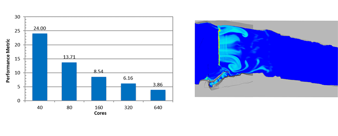
아래에는 물 및 환경, 금속 주조, 미세 유체 역학, 항공 우주 등 소프트웨어의 일반적인 응용 분야에 대한 HPC지원 FLOW-3D v12.0의 성능 분석 및 최대 2560개 코어까지 확장되는 것으로 나타난 lid-drived캐비티 시뮬레이션에 대한 전형적인 CFD벤치 마크 검증이 나와 있다.
이 시뮬레이션에서 유압 점프와 레일 위의 전체 흐름이 연구되었습니다. 메쉬:146만개 셀 실제 모델: 동적으로 계산된 최대 난류 혼합 길이의 자유 표면 추적, 중력, 공기 침투 및 RNG난류 모델 수치 모델:GMRERE
고압 분사–엔진 블록
이 시뮬레이션에서는 엔진 블록의 중력 주조를 연구했습니다. 메쉬:360만개 셀 물리적 모델: 자유 표면 추적, 중력, 열 전달, 응고 및 점성 층류 수치 모델:GMRERE
마이크로 데이터–PrinterNOZ내의 INKDROP LE
이 시뮬레이션에서 프린터 노즐의 잉크 방울의 형성과 배출을 연구했습니다. 메쉬:200만개 셀 물리적 모델: 자유 표면 추적, 층류 점성 및 표면 장력 수치 모델:GMRERE
AEROspace–항공기 연료 탱크 부싱
이 시뮬레이션에서는 다양한 비행 조건에서 F-16항공기 연료 탱크에서 연료 슬로싱을 연구했다. 메쉬:0.7만개 셀 물리적 모델: 동적으로 계산된 최대 난류 혼합 길이를 가진 자유 표면 추적, 비이상적 기준 프레임, 중력, 전기 전위 및 RNG난류 모델 수치 모델: ImplicitAdvection, GMrrs 및 분할 LagrangianVOF
BestCaseSCENARIO–LiDDrivenCavity
표준 뚜껑 구동 공동 문제는 FLow-3D의 스케일링 잠재력을 보여 주기 위해 시뮬레이션되었다. 이 시뮬레이션은 표준 CFD코드 검증에 자주 사용되는 완전하게 채워진 완벽한 부하 분산 시뮬레이션입니다. 메쉬:10.0만 셀 물리적 모델: 점성과 RNG난류. 수치 모델:GMRERE
자세한 내용은 STI C&D 솔루션팀에 문의하시기 바랍니다. flow3d@stikorea.co.kr or 02-2026-0455, 02-2026-0450.
FlowSight는 FLOW-3D및 FLOW-3D CAST결과의 정교한 시각화를 제공하도록 설계된 고급 후 처리 도구입니다. FlowSight는 직관적인 후처리 인터페이스 내에서 우수한 결과 분석 기능을 갖춘 모델을 제공합니다. 스플 라인 경로를 따라 임의의 2D클립, 3D클립 및 투명도, 볼륨 렌더링, 고급 데이터 타임 시리즈 플로팅, 간소화 및 벡터 플롯은 사용 가능한 놀라운 도구의 일부에 불과합니다. FlowSight를 사용하면 여러 뷰 포트와 동적 객체 시각화 도구로 구성된 풍부한 기능 세트와 결합되어 있으므로 엔지니어는 분석 및 프레젠테이션 요구 사항에 맞게 CFD결과를 최대한 활용할 수 있습니다.
FlowSight는 모든 FLOW-3D및 FLOW-3D CAST라이센스에 포함되어 추가비용 없이 사용할 수 있습니다.
새로운–스플 라인 클립!
FlowSight의 스플라인 클립 기능을 사용하면 복잡한 곡면을 따라 클립을 생성할 수 있습니다. ogee weir 위로 물이 흐르는 시뮬레이션에서, 스플 라인은 ogee weir의 표면을 따라 형성됩니다. 그런 다음 스플 라인이 돌출되어 웨어 표면을 따라 물의 자유 표면 높이에 의해 색상이 지정된 클립을 생성합니다.
키 프레임 기능
https://youtu.be/Hvg_ApXSu5g
크고 복잡한 시뮬레이션을 분석 할 때 매우 일반적인 문제는 관심 영역이 형상에 의해 가려지거나 시뮬레이션이 시간이 지남에 따라 변경됨에 따라 관심 영역이 변경 될 수 있다는 것입니다. 키 프레임은 분석 중에 형상을 “분리되도록”허용하고 시점이 시간과 공간을 통해 이동할 수 있도록 하여 이 문제를 해결합니다.
이 애니메이션은 FlowSight의 키 프레임 기능을 사용하여 충전하는 동안 다이 반쪽을 “시각적으로”열고 다이를 채우는 금속을 표시하면서 다이 표면에 고체 온도를 표시하는 방법을 보여줍니다.
Particle Visualization
FlowSight는 파티클(입자) 시각화 기능을 완벽하게 갖추고 있습니다. 입자는 입자 직경, 입자 밀도, 입자 수명, 속도 및 관련성이 있는 기타 변수에 의해 색상이 지정될 수 있습니다. 이 경우, 입자는 각각의 직경의 크기에 의해 착색됩니다.
속도 벡터 필드
FlowSight는 사용자에게 평면 또는 도메인 전체에 걸친 전체 볼륨 속도 및 방향 분석에 속도 벡터 필드를 시각화하는 옵션을 제공합니다. 사용자 지정 가능한 벡터 필드를 사용하면 다양한 색상 지정 및 밀도 조정이 가능하여 선명도를 높일 수 있습니다.
Streamlines & Pathlines
FlowSight의 유선(Streamlines) 기능은 복잡한 동적 패턴을 완전한 충실도로 시각화하여 유동장 속도 방향에 대해 실시간 스냅 샷을 제공합니다. 경로 선(Pathlines)은 시간을 따른 유체 입자의 궤적을 시뮬레이션하는 동안, 히스토리 라인은 유동장에서 유체 입자를 애니메이션 합니다.
Iso-surfaces
Iso-surfaces 은 유체 및 고체 표면을 시각화하는 강력하고 빠른 방법으로, 일정한 난류 에너지 영역을 표시하는 데 적합합니다.
Volume Render
iso-surface에서만 변수를 표시하는 대신 사용자 지정 가능한 볼륨 맵을 사용하여 볼륨 전체에 걸쳐 변수를 표시합니다. 그림에 표시된 바와 같이 각 기포와 주변 액체의 변형률 크기는 볼륨 렌더링과 함께 표시됩니다.
Multiple Data Views
숫자 및 다양한 그래프 등의 시각적 형식으로 분석하기
Visualizing Non-inertial Reference Frame Motion
Non-inertial reference frame visualization는 편리한 시뮬레이션 설정을 제공하고 계산 시간을 단축하며 사용자가 사실적인 방식으로 모델을 시각화 할 수 있게합니다.
https://youtu.be/DvKxNa1gOVs
2D Clips
2D 클립은 모든 단면 평면에서 유체 매개 변수를 시각화하는 데 사용됩니다.
3D Clipping
3D 클리핑 도구를 사용하면 사용자가 6 개 방향 모두에서 등면을 동시에 슬라이스 할 수 있으며, 높은 결함 영역을 감지하고 유체 및 고체 영역 내부의 온도, 압력, 속도 프로파일을 시각화하는 데 유용합니다.
특정 방향의 범위 사이에 애니메이션 제공
한 번에 한 방향으로 스왑
양방향 애니메이션 : 앞으로 및 뒤로
Arbitrary Clips
평면, 원통형, 상자, 원뿔형, 구형 및 간소화된 표면에 대한 시각화를 포함하여 광범위한 유연성으로 표면 뷰를 분석할 수 있습니다. 유체 흐름이 평면이 아닌 표면에 대한 시각화가 필요한 경우 유용합니다. 임의 클립을 사용하면 연속적으로 여러 클립을 만들 수도 있습니다.
Probe Data
포인트 프로브는 시간에 따른 변수의 진화를 보여주고, 라인 프로브는 거리에 따른 변수 값의 변화를 반환합니다. 오른쪽, 프로브는 유체의 응고 비율을 보여줍니다.
Vortex Cores
와류 코어 식별에 사용할 수있는 두 가지 옵션인 와류 및 고유 분석을 통해 코어 강도에 따라 필터링 가능한 결과 생성이 가능합니다.
엔지니어들은 연구를 위해 다양한 시각화 방법을 사용합니다. 유체 흐름에서 와류 코어의 분석은 중요한 문제로, 와류 코어는 속도 필드 내에 와류 구조 (중앙 트레이스)를 나타내는 선 입니다. 기술적으로, FlowSight는 와류 방법 및 고유치 분석에서 속도 벡터와 소용돌이 벡터의 속도장에서의 식별위치는 평행합니다. FlowSight는 사용자에게 와류 코어 식별을 위한 두 가지 옵션을 제공합니다. 코어는 특정 강도 이상 또는 이하로 FlowSight에서 필터링 될 수 있습니다. 코어는 일반적으로 코어 주위에 회전 또는 단순히 순환 강도의 비율에 의해 채색됩니다. 아래의 예에서는, 와류 코어 고유치 값 분석을 이용하여 생성됩니다. 강한 코어는 소용돌이의 중심에 형성되어있는 것을 알 수 있습니다. 이를 통해 사용자는 펌프로 공기 흡입의 가능성을 연구 할 수 있습니다. 코어가 너무 강한 경우, 공기는 강한 와류로 인해 야기되는 열린 통로로부터 흡입될 수 있습니다.
History Data
그래프 도구는 일반적인 히스토리, 진단 및 메시 종속 데이터에 강력한 수준의 분석을 제공하여 서로 다른 시뮬레이션 데이터를 상대적으로 보여줍니다.


 High flow condition hydraulic analysis of San Antonio river junction
 Simulation of a 6-km long reach of Fraser River in Vancouver, BC. Courtesy of Northwest Hydraulic Consultants. Image shows overall velocity flow field.
 A closer view of the piers of three bridge crossings. Courtesy of Northwest Hydraulic Consultants. Image shows velocity field around piers.
 Flows over submerged vanes for control of river bank erosion are shown colored by velocity magnitude (by University of Illinois; images generated with Tecplot)
 Simulation of the weir of the Third Dam on Somes Brook. Analysis of the fish passage was performed to appropriately repair structure so that the alewife can navigate it. Image colored by velocity magnitude.

 Manitoba Hydro에 의한 연구에 따르면, 사소한 설계 변경 사항이 있는 경우, 북부 Manitoba에 있는 Wuskwatim 수력발전 프로젝트의 3개의 게이트 인공 수로에서 측면 수축 효과가 실질적으로 감소될 수 있다고 합니다. 그 결과, 설계 수두가 실현되어 여수로 용량이 대략 5% 증가되었습니다. 이는 전체 공사 비용을 줄여주었습니다.